跳到论文正文
W Papers独立论文阅读器 arXiv:1605.02509 论文正文 计算阅读时间 · 0%
引用这篇论文根据当前论文元数据生成,正式投稿前建议核对。


License: arXiv.org perpetual non-exclusive license
arXiv:1605.02509v3 [math.CA] 03 Feb 2022

On the asymptotic behavior of Jacobi polynomials with first varying parameterThanks: The work is supported by the project ANR 18-CE40-0035

Oleg Szehr Address: Centre for Quantum Information, University of Cambridge, Cambridge CB3 0WA, United Kingdom. Address: Dalle Molle Institute for Artificial Intelligence (IDSIA) - SUPSI/USI, Manno, Switzerland Email address: oleg.szehr@idsia.ch and Rachid Zarouf Address: Aix-Marseille University, ADEF, University campus of Saint-Jérôme, 52 Avenue Escadrille Normandie Niemen, 13013 Marseille Email address: rachid.zarouf@univ-amu.fr Address: Department of Mathematics and Mechanics, Saint Petersburg State University, 28, Universitetski pr., St. Petersburg, 198504, Russia. Email address: rzarouf@gmail.com
Abstract.

We investigate the large nn behavior of Jacobi polynomials with varying parameters Pn(a​n+α,b​n+β)​(1−2​λ2)P_{n}^{(an+\alpha,\,bn+\beta)}(1-2\lambda^{2}) for a,b>−1a,b>-1 and λ∈(0, 1)\lambda\in(0,\,1). This is a well-studied topic in the literature but some of the published results appear to be discordant. To address this issue we provide an in-depth investigation of the case b=0b=0, which is most relevant for our applications. Our approach is based on a new and surprisingly simple representation of Pn(a​n+α,β)​(1−2​λ2),a>−1P_{n}^{(an+\alpha,\,\beta)}(1-2\lambda^{2}),\>a>-1 in terms of two integrals. The integrals’ asymptotic behavior is studied using standard tools of asymptotic analysis: one is a Laplace integral and the other is treated via the method of stationary phase. As a consequence we prove that if a∈(2​λ1−λ,∞)a\in(\frac{2\lambda}{1-\lambda},\infty) then λa​n​Pn(a​n+α,β)​(1−2​λ2)\lambda^{an}P_{n}^{(an+\alpha,\beta)}(1-2\lambda^{2}) shows exponential decay and we derive simple exponential upper bounds in this region. If a∈(−2​λ1+λ,2​λ1−λ)a\in(\frac{-2\lambda}{1+\lambda},\,\frac{2\lambda}{1-\lambda}) then the decay of λa​n​Pn(a​n+α,β)​(1−2​λ2)\lambda^{an}P_{n}^{(an+\alpha,\beta)}(1-2\lambda^{2}) is 𝒪(n−1/2)\mathcal{O}(n^{-1/2}) and if a∈{−2​λ1+λ,2​λ1−λ}a\in\{\frac{-2\lambda}{1+\lambda},\,\frac{2\lambda}{1-\lambda}\} then λa​n​Pn(a​n+α,β)​(1−2​λ2)\lambda^{an}P_{n}^{(an+\alpha,\beta)}(1-2\lambda^{2}) decays as 𝒪(n−1/3)\mathcal{O}(n^{-1/3}). A new phenomenon occurs in the parameter range a∈(−1,−2​λ1+λ)a\in(-1,\frac{-2\lambda}{1+\lambda}), where we find that the behavior depends on whether or not a​n+αan+\alpha is an integer: If a∈(−1,−2​λ1+λ)a\in(-1,\frac{-2\lambda}{1+\lambda}) and a​n+αan+\alpha is an integer then λa​n​Pn(a​n+α,β)​(1−2​λ2)\lambda^{an}P_{n}^{(an+\alpha,\beta)}(1-2\lambda^{2}) decays exponentially. If a∈(−1,−2​λ1+λ)a\in(-1,\frac{-2\lambda}{1+\lambda}) and a​n+αan+\alpha is not an integer then λa​n​Pn(a​n+α,β)​(1−2​λ2)\lambda^{an}P_{n}^{(an+\alpha,\beta)}(1-2\lambda^{2}) may increase exponentially depending on the proximity of the sequence (a​n+α)n(an+\alpha)_{n} to integers.

Key words and phrases:
Jacobi polynomials, Integral representation, Method of stationary phase, Laplace’s method.
2010 Mathematics Subject Classification: Primary: 33C45; Secondary: 30E15

1. Introduction

The Jacobi polynomials Pn(α,β)P_{n}^{(\alpha,\,\beta)} (occasionally also called hypergeometric polynomials) constitute a wide class of classical polynomials. They include the Gegenbauer and thus also the Legendre, Zernike and Chebyshev polynomials as special cases. For α,β∈ℝ\alpha,\beta\in\mathbb{R} and x∈(−1,1)x\in(-1,1) the Jacobi polynomials of degree nn can be defined [71, p. 68] by

Pn(α,β)​(x)=∑μ=0n(n+αn−μ)​(n+βμ)​(x−12)μ​(x+12)n−μ.\displaystyle P_{n}^{(\alpha,\,\beta)}(x)=\sum_{\mu=0}^{n}\binom{n+\alpha}{n-\mu}\binom{n+\beta}{\mu}\left(\frac{x-1}{2}\right)^{\mu}\left(\frac{x+1}{2}\right)^{n-\mu}.

This article is concerned with the approximation of large degree Jacobi polynomials. While for fixed parameters α,β\alpha,\beta this is a classical topic of asymptotic analysis and approximation theory [80, 71], this work is concerned with the more general Jacobi polynomials with varying parameters (JPVPs)

Pn(a​n+α,b​n+β)​(x),a,b,α,β>−1.P_{n}^{(an+\alpha,bn+\beta)}(x),\qquad{a,b,\alpha,\beta>-1}.

The asymptotic behavior of JPVPs has been the content of multiple preceeding publications including [14, 23, 32, 38, 41, 68, 20]. We have observed that some of the results are discordant, which led us to search for a simple and robust approach to the topic. The articles [20, 41, 68] investigate the case b=0b=0, i.e. only the first parameter of JPVPs depends on nn. We call such polynomials Jacobi polynomials with first varying parameter (JPFVPs). Our presentation is streamlined to this case because it is the most relevant for our applications and to allow for an immediate comparison to [20, 41, 68]. At the core of our investigation lies a new representation of Jacobi polynomials in terms of two integrals. The representation is chosen such that the integrals’ asymptotic behavior can be determined by means of well-established methods. The first integral is a generalized Fourier integral, whose asymptotic behavior follows from Erdélyi’s classical method of stationary phase [29]. The second integral is of Laplace type: its asymptotic behavior is determined by the classical method of Laplace [2, Section 6.4]. Thus we introduce a new and comparatively simple approach to the topic. Based on our integral representation we systematically determine the asymptotic behavior of JPFVPs and we explain how our method extends to the general case of JPVPs. The theoretical investigation is accompanied with extensive numerical experiments.

We find that the behavior of JPFVPs is non-trivial in the sense that different types of asymptotics occur as n→∞n\rightarrow\infty. To state the results it is convenient to change the variable of the polynomials writing x=1−2​λ2x=1-2\lambda^{2} with λ∈(0,1)\lambda\in(0,1). As we will prove in the main body of this article there are four distinct parameter regions, 1) a∈(−1,−2​λ1+λ)a\in(-1,\frac{-2\lambda}{1+\lambda}), 2) a∈(−2​λ1+λ,2​λ1−λ)a\in(-\frac{2\lambda}{1+\lambda},\,\frac{2\lambda}{1-\lambda}), 3) a∈(2​λ1−λ,∞)a\in(\frac{2\lambda}{1-\lambda},\infty) and 4) a∈{−2​λ1+λ,2​λ1−λ}a\in\left\{-\frac{2\lambda}{1+\lambda},\,\frac{2\lambda}{1-\lambda}\right\} with categorically different asymptotics. The below listing summarizes our findings in the respective cases and compares them to the literature.

  1. (1)

    The case a∈(−1,2​λ1−λ)a\in(-1,\frac{2\lambda}{1-\lambda}) has been studied in [23] and [41]. According to [41] the results of [23] must be corrected. [41] claims that if a∈(−1,2​λ1−λ)a\in(-1,\frac{2\lambda}{1-\lambda}) then the decay of λa​n​Pn(a​n+α,β)​(1−2​λ2)\lambda^{an}P_{n}^{(an+\alpha,\,\beta)}(1-2\lambda^{2}) is 𝒪(n−1/2)\mathcal{O}\left(n^{-1/2}\right). Our result, see Theorem 1 below, contradicts both [23] and [41]. For a∈(−1,−2​λ1+λ)a\in(-1,-\frac{2\lambda}{1+\lambda}) we identify a new form of asymptotic behavior:

    1. (a)

      If a​n+αan+\alpha is an integer then λa​n​Pn(a​n+α,β)​(1−2​λ2)\lambda^{an}P_{n}^{(an+\alpha,\,\beta)}(1-2\lambda^{2}) decays exponentially in magnitude.

    2. (b)

      If a​n+αan+\alpha remains strictly separate from integers on a subsequence of natural numbers then

      λa​n​Pn(a​n+α,β)​(1−2​λ2)\lambda^{an}P_{n}^{(an+\alpha,\beta)}(1-2\lambda^{2})

      increases exponentially in magnitude along this subsequence.

  2. (2)

    It is shown in [38, 32] that if a∈[0,2​λ1−λ)a\in\left[0,\frac{2\lambda}{1-\lambda}\right) then λa​n​Pn(a​n+α,β)​(1−2​λ2)\lambda^{an}P_{n}^{(an+\alpha,\beta)}(1-2\lambda^{2}) decays in first order like 𝒪(n−1/2)\mathcal{O}\left(n^{-1/2}\right). The wider interval a∈(−2​λ1+λ,2​λ1−λ)a\in(-\frac{2\lambda}{1+\lambda},\,\frac{2\lambda}{1-\lambda}) is studied in [41, 23], where a decay of 𝒪(n−1/2)\mathcal{O}\left(n^{-1/2}\right) is found. However, the explicit formulas of [41, 23] and [38, 32] are inconsistent. In this range of parameters our findings are identical to those of [38, Theorem 1] and to [32, Proposition 6.1] (but notice the different 𝒪\mathcal{O}-term, see Remark 3).

  3. (3)

    For a>2​λ1−λa>\frac{2\lambda}{1-\lambda} we find that λa​n​Pn(a​n+α,β)​(1−2​λ2)\lambda^{an}P_{n}^{(an+\alpha,\,\beta)}(1-2\lambda^{2}) decays exponentially which is in line with [41, 23], see Theorem 1 points (3) and (4) for details.

  4. (4)

    For a∈{−2​λ1+λ,2​λ1−λ}a\in\left\{-\frac{2\lambda}{1+\lambda},\,\frac{2\lambda}{1-\lambda}\right\} we find that λa​n​Pn(a​n+α,β)​(1−2​λ2)\lambda^{an}P_{n}^{(an+\alpha,\,\beta)}(1-2\lambda^{2}) decays in first order like 𝒪(n−1/3)\mathcal{O}(n^{-1/3}). Our asymptotic formulas, see Theorem 1 point (2) for details, differ from [23, Formula (3.9)]. This case is not investigated in [41]. An asymptotic formula is also derived in [68] for a=2​λ1−λa=\frac{2\lambda}{1-\lambda} but the printed formula differs from ours by a complex prefactor.

Our results cannot be directly compared to those obtained in [44, 50] because the authors are interested in a different range of parameters. [44] focuses on parameters that satisfy the following two conditions: −1<a<0-1<a<0, −1<b<0-1<b<0, a+b<−1a+b<-1 and α=β=0\alpha=\beta=0. [50] treats the case that a,ba,\,b are not both positive and take values outside the triangle bounded by a=0,b=0a=0,\,b=0 and a+b+2=0a+b+2=0 and α=β=0\alpha=\beta=0. But for negative values of a,ba,b their formulas witness a similar dependency on the proximity of (a+b)​n(a+b)n to an integer as the one we find in region 1), see for example [44, Theorem 2.6] and [44, Remark 2.9].

Our interest in the asymptotic behavior of Jacobi polynomials arose from their relation to the Fourier coefficients of the Blaschke product B=bn=(z−λ1−λ​z)nB=b^{n}=\left(\frac{z-\lambda}{1-\lambda z}\right)^{n}. In fact the kt​hk^{th} Fourier coefficient of BB is given by

(1.1) B^​(k)=λk−n​(1−λ2)​Pn−1(k−n, 1)​(1−2​λ2),\displaystyle\hat{B}(k)=\lambda^{k-n}(1-\lambda^{2})P_{n-1}^{(k-n,\,1)}(1-2\lambda^{2}),

which is a consequence of Lemma 2 below. Being the nn-th power of the disk automorphism, BB plays a key role in the operator theory of holomorphic Banach spaces of the unit disk. Consider, for instance, the classical Beurling-Sobolev space

lpA​(w):={f=∑k≥0f^​(k)​zk∈H​o​l​(𝔻)|‖f‖lpA​(w):=(∑k≥0|f^​(k)|p​wkp)1/p<∞},l_{p}^{A}(w):=\left\{f=\sum_{k\geq 0}\hat{f}(k)z^{k}\in Hol(\mathbb{D})\>\Big|\>\left|\!\left|f\right|\!\right|_{l_{p}^{A}(w)}:=\left(\sum_{k\geq 0}|\hat{f}(k)|^{p}w_{k}^{p}\right)^{1/p}<\infty\right\},

where the sequence of weights w=(wk)k≥1w=(w_{k})_{k\geq 1} is such that wk>0w_{k}>0, limkwk1/k=1\lim_{k}w_{k}^{1/k}=1 [56, p. 670]. We write briefly lpAl_{p}^{A} for the special case of the analytic sequence space, w=(1)k≥1w=(1)_{k\geq 1}. The asymptotic nn-dependency of ‖B‖lpA​(w)\left|\!\left|B\right|\!\right|_{l_{p}^{A}(w)} is connected to the asymptotics of JPFVPs via Equation (1.1) because the asymptotic analysis requires the investigation of regions of Fourier coefficients where kk is proportional to nn. The regions 1), 2), 3), 4) typically play different roles in terms of their contribution to ‖B‖lpA​(w)\left|\!\left|B\right|\!\right|_{l_{p}^{A}(w)}. The region of exponential decay of |B^​(k)||\hat{B}(k)| adds an asymptotically negligible contribution. Simple exponential upper estimates are a therefore a useful tool to restrict the analysis to the relevant coefficients. In general, it will depend on ww and pp, which region contributes the terms that dominate the asymptotic behavior.

We illustrate the relevance of information about the asymptotic behavior of ‖B‖lpA​(w)\left|\!\left|B\right|\!\right|_{l_{p}^{A}(w)} by some examples. First, the asymptotic behavior of ‖B‖lpA\left|\!\left|B\right|\!\right|_{l_{p}^{A}}, p∈[1,2]p\in[1,2], has been determined in [8] to study the boundedness of composition operators (c​o​m​pb​(f))​(z):=f⁡(b⁡(z))(comp_{b}(f))(z):=f(b(z)) on lpAl_{p}^{A}. In similar spirit, information about ‖B‖lpA​(w)\left|\!\left|B\right|\!\right|_{l_{p}^{A}\left(w\right)} has recently been exploited in [47] to identify the sequences w=(wk)k≥1w=(w_{k})_{k\geq 1}, for which the composition operator on the weighted Hardy space l2A​(w)l_{2}^{A}(w) is bounded. We have computed the exact asymptotic nn-dependency of ‖B‖lpA\left|\!\left|B\right|\!\right|_{l_{p}^{A}} for p∈[1,∞]p\in[1,\infty] in [77]. Second, ‖B‖lpA​(w)\left|\!\left|B\right|\!\right|_{l_{p}^{A}(w)} plays an important role in interpolation theory: Consider the formal Hölder inequality

|⟨f|g⟩|≤‖f‖lqA​‖g‖lpA|\langle f|g\rangle|\leq\left|\!\left|f\right|\!\right|_{l_{q}^{A}}\left|\!\left|g\right|\!\right|_{l_{p}^{A}}

where 1/p+1/q=11/p+1/q=1 and ⟨⋅|⋅⟩\langle\cdot|\cdot\rangle denotes the usual scalar product on L2​(∂𝔻)L^{2}(\partial\mathbb{D}). For the Nevanlinna-Pick-type interpolation problem [56] in lqAl_{q}^{A} with (λi)i=1n⊂𝔻(\lambda_{i})_{i=1}^{n}\subset\mathbb{D},

ℐ=inf{||f||lqA:f(0)=1,f(λi)=0,i=1,…,n},\mathcal{I}=\inf\{\left|\!\left|f\right|\!\right|_{l_{q}^{A}}:f(0)=1,\ f(\lambda_{i})=0,\ i=1,...,n\},

choosing g=Bg=B, where BB is the Blaschke product associated to the sequence (λi)i=1n(\lambda_{i})_{i=1}^{n}, entails the lower estimate

ℐ≥1Πi=1n​|λi|​‖B‖lpA.\mathcal{I}\geq\frac{1}{\Pi_{i=1}^{n}|\lambda_{i}|\left|\!\left|B\right|\!\right|_{l_{p}^{A}}}.

In other words any ff that is admissible for ℐ\mathcal{I} grows at least as quickly as 1/(Πi=1n​|λi|​‖B‖lpA)1/({\Pi_{i=1}^{n}|\lambda_{i}|\left|\!\left|B\right|\!\right|_{l_{p}^{A}}}). The same reasoning extends mutatis mutandis to the more general Beurling-Sobolev spaces lpA​(w)l_{p}^{A}(w). Third, the norm ‖B‖lpA​(w)\left|\!\left|B\right|\!\right|_{l_{p}^{A}(w)} occurs in extremal problems in matrix analysis. While an introduction to model theory would lead beyond the scope of this article (see [53] for details) we briefly illustrate the flavor of problems in this area. Suppose AA is a complex n×nn\times n matrix with spectrum (λi)i=1n(\lambda_{i})_{i=1}^{n}, ||⋅||\left|\!\left|\cdot\right|\!\right| an induced matrix norm with ‖A‖≤1\left|\!\left|A\right|\!\right|\leq 1, and let ψ\psi be any rational function, whose poles are disjoint from the eigenvalues of AA. Consider the extremal problem

ℰ=sup‖ψ⁡(T)‖,\displaystyle\mathcal{E}=\sup\left|\!\left|\psi(T)\right|\!\right|,

where the supremum goes over all TT with ‖T‖≤1\left|\!\left|T\right|\!\right|\leq 1 that have the same minimal polynomial as AA. Then it holds [56, 74]

(1.2) ℐ=inf{||f||l1A|​f​(λi)=ψ⁡(λi),i=1,…,n}=‖ψ⁡(M)‖≤ℰ,\displaystyle\mathcal{I}=\inf\{|\!|f|\!|_{l_{1}^{A}}\>|\>f(\lambda_{i})=\psi(\lambda_{i}),i=1,...,n\}=\left|\!\left|\psi(M)\right|\!\right|\leq\mathcal{E},

where MM is an operator model of AA: MM has the same minimal polynomial as AA and ‖M‖≤1\left|\!\left|M\right|\!\right|\leq 1, too. Thus, the techniques to bound ℐ\mathcal{I} from below are also available for the estimation of ℰ\mathcal{E}. This method has been employed (for ψ⁡(z)=z−1\psi(z)=z^{-1}) to introduce a constructive approach to a conjecture of Schäffer [74]. In similar vein, there is an open question of V. Pták [86, 65] from the 1980’s: Over all n×nn\times n complex matrices AA with ‖A‖2≤1\left|\!\left|A\right|\!\right|_{2}\leq 1, where ||⋅||2\left|\!\left|\cdot\right|\!\right|_{2} is the Hilbert space operator norm, and with spectral radius bounded by λ∈(0,1)\lambda\in(0,1) determine the supremum of ‖An‖2\left|\!\left|A^{n}\right|\!\right|_{2} as a function of nn and λ\lambda. It is shown in [65] that the supremum is attained by the model operator whose spectrum (λi)i=1n(\lambda_{i})_{i=1}^{n} is fully degenerate at point λ\lambda. As it turns out the entries of the NN-th power of the model operator can be expressed (in Malmquist-Walsh basis [53, p. 117]) as

(MN)i,j={(−λ)i−j−N​(1−λ2)​PN−1(i−j−N,1)​(1−2​λ2),i>j,λN,i=j,0,i<j,\displaystyle\left(M^{N}\right)_{i,j}=\begin{cases}(-\lambda)^{i-j-N}(1-\lambda^{2})P_{N-1}^{(i-j-N,1)}(1-2\lambda^{2}),\ &i>j,\\ \lambda^{N},\ &i=j,\\ 0,\ &i<j,\end{cases}

which relates Pták’s question to the theory of JPFVPs by (1.2).

Section 2 contains our main results. Our insights about the asymptotic behavior of JPFVPs are presented in Section 2.1 and our new integral representation for JPFVPs in Section 2.2. Section 3 describes our methods to determine the asymptotic behavior of the involved integrals. The generalized Fourier integral is treated in Section 3.1 and the Laplace integral in Section 3.2. Section 4 provides simple exponential estimates for the JPFVPs in the region of exponential decay/ growth. The proof of our main theorem is given in Section 5. Section 6 contains the results of our numerical experiments. Building on our integral representation Section 7 describes possible generalizations of our work. This includes the case of JPVPs with b≠0b\neq 0 and a description of the methodology to obtain uniform asymptotic expansions as aa approaches the boundaries.

acknowledgments

The authors are grateful to A. D. Baranov, A. A. Borichev, S. Charpentier, S. Kupin for their comments on an earlier version of our manuscript.

2. Main results

2.1. On the asymptotic behavior of Jacobi polynomials with first varying parameter

Theorem 1.

Let α,β>−1\alpha,\ \beta>-1, a>−1a>-1 and λ∈(0, 1)\lambda\in(0,\,1). The following asymptotic formulas hold as n→∞n\rightarrow\infty:

  1. (1)

    If a∈(−2​λ1+λ,2​λ1−λ)a\in(-\frac{2\lambda}{1+\lambda},\,\frac{2\lambda}{1-\lambda}) then

    λa​n+α​Pn(a​n+α,β)​(1−2​λ2)=2n​π​((1−λ2)​(a+1))−β2((1−λ2)​((a+2)​λ+a)​((a+2)​λ−a))14\displaystyle\lambda^{an+\alpha}P_{n}^{(an+\alpha,\,\beta)}(1-2\lambda^{2})=\sqrt{\frac{2}{n\pi}}\frac{((1-\lambda^{2})(a+1))^{-\frac{\beta}{2}}}{((1-\lambda^{2})((a+2)\lambda+a)((a+2)\lambda-a))^{\frac{1}{4}}}
    ⋅cos⁡((n+1)​h​(φ+)+(α−a)​φ++(β−1)​ψ+π4)+𝒪⁡(1n3/2).\displaystyle\cdot\cos{\left((n+1)h(\varphi_{+})+(\alpha-a)\varphi_{+}+(\beta-1)\psi{+}\frac{\pi}{4}\right)}+\mathcal{O}\left(\frac{1}{n^{3/2}}\right).

    The phases φ+,h(φ+),ψ∈(−π,π]\varphi_{+},h(\varphi_{+}),\psi\in(-\pi,\pi] depend on a,λa,\lambda and are given explicitly in Proposition 3 below.

  2. (2)

    If a=2​λ1−λa=\frac{2\lambda}{1-\lambda} then

    λa​n+α​Pn(a​n+α,β)​(1−2​λ2)=(1+λ)−β32/3​Γ​(2/3)​n1/3​λ1/3​(1+λ)1/3​(1+𝒪⁡(1n1/3)).\displaystyle\lambda^{an+\alpha}P_{n}^{(an+\alpha,\,\beta)}(1-2\lambda^{2})=\frac{(1+\lambda)^{-\beta}}{3^{2/3}\Gamma(2/3)n^{1/3}\lambda^{1/3}(1+\lambda)^{1/3}}\left(1+\mathcal{O}\left(\frac{1}{n^{1/3}}\right)\right).

    If a=−2​λ1+λa=-\frac{2\lambda}{1+\lambda} then

    λa​n+α​Pn(a​n+α,β)​(1−2​λ2)=(1−λ)−β32/3​Γ​(2/3)​π​n1/3​λ1/3​(1−λ)1/3\displaystyle\lambda^{an+\alpha}P_{n}^{(an+\alpha,\,\beta)}(1-2\lambda^{2})=\frac{(1-\lambda)^{-\beta}}{3^{2/3}\Gamma(2/3)\pi n^{1/3}\lambda^{1/3}(1-\lambda)^{1/3}}
    ⋅(cos⁡((a​n+α)​π)−3​sin⁡((a​n+α)​π))+𝒪⁡(1n2/3).\displaystyle\cdot\left(\cos\left((an+\alpha)\pi\right)-\sqrt{3}\sin\left((an+\alpha)\pi\right)\right)+\mathcal{O}\left(\frac{1}{n^{2/3}}\right).
  3. (3)

    If a∈(−1,−2​λ1+λ)∪(2​λ1−λ,∞)a\in(-1,\frac{-2\lambda}{1+\lambda})\cup(\frac{2\lambda}{1-\lambda},\infty) and a​n+αan+\alpha is an integer then the quantity

    λa​n+α​Pn(a​n+α,β)​(1−2​λ2)\lambda^{an+\alpha}P_{n}^{(an+\alpha,\,\beta)}(1-2\lambda^{2})

    decays exponentially in magnitude with nn, see Proposition 6 for an upper bound.

  4. (4)

    If a∈(−1,−2​λ1+λ)a\in(-1,-\frac{2\lambda}{1+\lambda}) and if the sequence (a​n+α)n(an+\alpha)_{n} is separate from integers then the quantity

    λa​n+α​Pn(a​n+α,β)​(1−2​λ2)\lambda^{an+\alpha}P_{n}^{(an+\alpha,\,\beta)}(1-2\lambda^{2})

    increases exponentially in magnitude. The precise behavior depends on the proximity of the sequence (a​n+α)n(an+\alpha)_{n} to integers, see the proof of Theorem 1 point (4). If a∈(2​λ1−λ,∞)a\in(\frac{2\lambda}{1-\lambda},\infty) and a​n+αan+\alpha is not an integer then the above quantity decays exponentially in magnitude.

Remark 1.

Our approach to prove points 1), 2) can also be used to derive asymptotic formulas in the exponential region a∈(−1,−2​λ1+λ)∪(2​λ1−λ,∞)a\in(-1,\frac{-2\lambda}{1+\lambda})\cup(\frac{2\lambda}{1-\lambda},\infty), see Section 5. We prefer the shorter formulation here, because it is sufficient for our application.

Remark 2.

The developed methodology yields an expansion of Pn(a​n+α,β)​(1−2​λ2)P_{n}^{(an+\alpha,\,\beta)}(1-2\lambda^{2}) to any order. The required computations are straight-forward albeit tedious.

Remark 3.

Determining the precise asymptotic growth of the JPVFPs can be a delicate task in cases, where the formulas involve oscillating trigonometric functions of nn. To illustrate the phenomenon consider the oscillating term

2n​π​cos⁡(((n+1)​h​(φ+)+(α−a)​φ++(β−1)​ψ+π4)CLOSE\sqrt{\frac{2}{n\pi}}\cos\left(((n+1)h(\varphi_{+})+(\alpha-a)\varphi_{+}+(\beta-1)\psi{+}\frac{\pi}{4}\right)

in 1), which is clearly 𝒪⁡(1/n)\mathcal{O}(1/\sqrt{n}). While the second summand in 1) is only 𝒪⁡(1/n3)\mathcal{O}(1/\sqrt{n^{3}}) it is still not obvious, which term actually provides the dominating contribution to the JPFVPs. For completeness we show in Section 5 that given γ∈ℝ\gamma\in\mathbb{R} there exists a subsequence sn∈ℕs_{n}\in\mathbb{N} such that |cos⁡(γ​sn+π2)|≤K/sn|\cos(\gamma s_{n}+\frac{\pi}{2})|\leq K/s_{n} with a constant KK. Notice that along such a subsequence the oscillating term can be 𝒪⁡(1/n3)\mathcal{O}(1/\sqrt{n^{3}}).

The theorem is an immediate consequence of our representation of the JPFVPs in terms of two integrals, Lemma 2, together with the asymptotic formulas for the individual integrals, Proposition 3 and Proposition 5. The results are collected in Section 5. Various methods are employed in the literature to prove asymptotic expansions. Gawronksi-Shawyer [38] as well as Saff-Varga [68] rely on the method of steepest descent [2, p. 147] [59, p. 136], while Chen-Ismail [23] and Izen [41] make use of Darboux’s asymptotic method and generating functions [59, 71]. In this article classical methods of asymptotic analysis are employed to determine the asymptotic behavior of our integral representation. Even in situations when no integral representation is available, the Riemann-Hilbert approach [44, 50] can still be employed to derive asymptotic expansions. The Riemann-Hilbert approach has the additional advantage that it automatically provides uniform (over a,b,λa,b,\lambda) asymptotic expansions. A uniform expansion can also be obtained from our integral representation using well-established methods, see Section 7.2, although this is not the main focus of the article.

2.2. A new integral representation for Jacobi Polynomials

Although simple, we regard the below lemma as the main innovation of this work. In what follows powers are defined with respect to the principal branch of the complex logarithm, which is denoted by Log\Log.

Lemma 2 (Integral representation for JPFVPs).

Let nn be an integer, let a>−1a>-1 and α,β∈ℝ\alpha,\,\beta\in\mathbb{R} be such that (a+1)​n+α>−1(a+1)n+\alpha>-1. Given λ∈(0, 1)\lambda\in(0,\,1), for any x∈(λ, 1/λ)x\in(\lambda,\,1/\lambda) we have the following integral representation for the Jacobi polynomials with first varying parameter

λa​n+α​(1−λ2)β​Pn(a​n+α,β)​(1−2​λ2)\displaystyle\lambda^{an+\alpha}(1-\lambda^{2})^{\beta}P_{n}^{(an+\alpha,\,\beta)}(1-2\lambda^{2})
=1π​ℜ⁡{∫0πzα+1​(1−λ​z)βz−λ​(za+1​(1−λ​z)z−λ)n|z=x​ei​φ​d​φ}\displaystyle=\frac{1}{\pi}\Re\left\{\int_{0}^{\pi}{z^{\alpha+1}\frac{(1-\lambda z)^{\beta}}{z-\lambda}\bigg(z^{a+1}\frac{(1-\lambda z)}{z-\lambda}\bigg)^{n}}\Bigg|_{z={x}e^{i\varphi}}\textnormal{d}\varphi\right\}
−sin⁡(π⁡(a​n+α))π∫0x(1+λ​t)β​tαt+λ(t(a+1)(1+λ​t)t+λ)ndt,\displaystyle-\frac{{\sin\left(\pi(an+\alpha)\right)}}{\pi}\int_{0}^{{x}}\frac{(1+\lambda t)^{\beta}t^{\alpha}}{t+\lambda}\left(t^{(a+1)}\frac{(1+\lambda t)}{t+\lambda}\right)^{n}{\rm d}t,

where ℜ⁡(∙)\Re(\bullet) stands for the real part of a complex number.

This representation is particularly suited for asymptotic analysis.

  1. (1)

    The first integral can be written as a so-called generalized Fourier integral [29], [2, Chapter 6.5]. The latter is of the form

    ∫g⁡(φ)​ei​n​h​(φ)​d​φ\int g(\varphi)e^{inh(\varphi)}\textnormal{d}\varphi

    with continuous and real functions gg, hh. To determine the asymptotic behavior we employ the method of stationary phase, which is commonly used to study asymptotic properties of oscillatory integrals. The method is conceptually similar to Laplace’s method (see below) in that the leading order terms are contributed by a small neighborhood around the stationary points of hh. Our analysis relies on the well-known fact [29, Theorem 4], [2, Chapter 6.5] that if ξ\xi is a stationary point of hh such that g⁡(ξ)≠0g(\xi)\neq 0 then

    1. (a)

      the integral goes to 0 as n−1/2n^{-1/2} if h′′​(ξ)≠0h^{\prime\prime}(\xi)\neq 0,

    2. (b)

      the integral goes to 0 as n−1/3n^{-1/3} if h′′​(ξ)=0h^{\prime\prime}(\xi)=0 but h(3)​(ξ)≠0h^{(3)}(\xi)\neq 0.

  2. (2)

    The second integral contributes iff a​n+αan+\alpha is not an integer and is of Laplace type [59, Chapter 3]. The latter is of the form

    ∫g⁡(t)​en​h​(t)​d​t,\int g(t)e^{nh(t)}\textnormal{d}t,

    with continuous and real functions gg, hh. To determine the asymptotic behavior we employ Laplace’s method. The idea is that if hh has a maximum at ξ\xi and if g⁡(ξ)≠0g(\xi)\neq 0 then as nn grows only values in an immediate neighborhood of ξ\xi contribute [2, 59].

Curiously the second integral contributes iff a​n+αan+\alpha is not an integer. As a consequence the magnitude of JPFVPs “scatters” as a function of nn depending on (a,α)(a,\alpha). To determine the asymptotic behavior it is therefore necessary to consider subsequences of nn. On a subsequence of nn where a​n+αan+\alpha is an integer the second integral does never contribute. However for such nn that a​n+αan+\alpha is not an integer the second integral contributes, which potentially alters the asymptotic behavior in a “discontinuous” way.

Proof.

We investigate the complex function

f:z↦z(a+1)​n+α​(1−λ​z)n+β(z−λ)n+1.f:z\mapsto z^{(a+1)n+\alpha}\frac{(1-\lambda z)^{n+\beta}}{(z-\lambda)^{n+1}}.

We integrate ff along a closed contour γ\gamma in the complex plane, see Figure 2.1. The contour is composed of four curves γ=γ1⊕γ2⊕γ3⊕γ4\gamma=\gamma_{1}\oplus\gamma_{2}\oplus\gamma_{3}\oplus\gamma_{4} with x∈(λ,1/λ)x\in(\lambda,1/\lambda) and

γ1\displaystyle\gamma_{1} :φ↦xei​φ,φ∈(−π,π],\displaystyle:\varphi\mapsto xe^{i\varphi},\quad\varphi\in(-\pi,\pi],
γ2\displaystyle\gamma_{2} :φ↦ϵe−i​φ,φ∈(−π,π],\displaystyle:\varphi\mapsto\epsilon e^{-i\varphi},\quad\varphi\in(-\pi,\pi],
γ3\displaystyle\gamma_{3} :t↦t+i​ϵ~,t∈[−x,0],\displaystyle:t\mapsto t+i\tilde{\epsilon},\quad t\in[-x,{0}],
γ4\displaystyle\gamma_{4} :t↦−t−i​ϵ~,t∈[0,x].\displaystyle:t\mapsto-t-i\tilde{\epsilon},\quad t\in[0,{x}].
γ2\gamma_{2}γ1\gamma_{1}γ3\gamma_{3}γ4\gamma_{4}γ5\gamma_{5}λ\lambda11
Figure 2.1. Contours γ=γ1⊕γ2⊕γ3⊕γ4\gamma=\gamma_{1}\oplus\gamma_{2}\oplus\gamma_{3}\oplus\gamma_{4} and γ5\gamma_{5} for x=1x=1.

Due to holomorphy we have that

12​π​i​∫γ1⊕γ2⊕γ3⊕γ4f​d​z=12​π​i​∫γ5f​d​z,\displaystyle\frac{1}{2\pi i}\int_{\gamma_{1}\oplus\gamma_{2}\oplus\gamma_{3}\oplus\gamma_{4}}f\ \textnormal{d}z=\frac{1}{2\pi i}\int_{\gamma_{5}}f\ \textnormal{d}z,

where γ5\gamma_{5} denotes a small circle around the pole λ\lambda, see Figure 2.1,

γ5:φ↦λ+sei​φ,φ∈(−π,π].\displaystyle\gamma_{5}:\varphi\mapsto\lambda+se^{i\varphi},\ \varphi\in(-\pi,\pi].

The lemma is proved by computing each of the five integrals individually.

  • •

    We observe that

    12​π​i​∫γ1f​d​z\displaystyle\frac{1}{2\pi i}\int_{\gamma_{1}}f\ \textnormal{d}z =12​π​∫−ππz(a+1)​n+α+1​(1−λ​z)n+β(z−λ)n+1|z=x​ei​φ​d​φ\displaystyle=\frac{1}{2\pi}\int_{-\pi}^{\pi}z^{(a+1)n+\alpha+1}\frac{(1-\lambda z)^{n+\beta}}{(z-\lambda)^{n+1}}\Bigg|_{z={x}e^{i\varphi}}\textnormal{d}\varphi
    =1π​ℜ⁡{∫0πz(a+1)​n+α+1​(1−λ​z)n+β(z−λ)n+1|z=x​ei​φ​d​φ}.\displaystyle=\frac{1}{\pi}\Re\left\{\int_{0}^{\pi}{z^{(a+1)n+\alpha+1}\frac{(1-\lambda z)^{n+\beta}}{(z-\lambda)^{n+1}}}\Bigg|_{z={x}e^{i\varphi}}\textnormal{d}\varphi\right\}.
  • •

    The standard estimate for contour integrals reads

    |12​π​i​∫γ2f​d​z|\displaystyle\left|\frac{1}{2\pi i}\int_{\gamma_{2}}f\ \textnormal{d}z\right| ≤ϵ​maxz∈γ2​|z(a+1)​n+α+1​(1−λ​z)n+β(z−λ)n+1|\displaystyle\leq\epsilon\max_{z\in\gamma_{2}}\left|z^{(a+1)n+\alpha+1}\frac{(1-\lambda z)^{n+\beta}}{(z-\lambda)^{n+1}}\right|
    ≤ϵ(a+1)​n+α+2​maxz∈γ2​|(1−λ​z)n+β(z−λ)n+1|,\displaystyle\leq\epsilon^{(a+1)n+\alpha+2}\max_{z\in\gamma_{2}}\left|\frac{(1-\lambda z)^{n+\beta}}{(z-\lambda)^{n+1}}\right|,

    which goes to 00 as ϵ→0\epsilon\rightarrow 0.

  • •

    We have zy=ey​Log⁡(z)=ey​|z|+i​y​Arg⁡(z)z^{y}=e^{y\Log(z)}=e^{y|z|+iy\Arg(z)} with the main branch of the argument and so

    ∫γ3f​d​z\displaystyle\int_{\gamma_{3}}f\ \textnormal{d}z =∫−x0z(a+1)​n+α​(1−λ​z)βz−λ​(1−λ​zz−λ)n|z=t+i​ε~​d​t\displaystyle=\int_{-x}^{0}z^{(a+1)n+\alpha}\frac{(1-\lambda z)^{\beta}}{z-\lambda}\left(\frac{1-\lambda z}{z-\lambda}\right)^{n}\Bigg|_{z=t+i\tilde{\varepsilon}}\textnormal{d}t
    →ε~→0∫−x0|t|(a+1)​n+α​e((a+1)​n+α)​π​i​|1−λ​t|β|t|​eπ​i−λ​(1−λ​|t|​eπ​i|t|​eπ​i−λ)n​d​t\displaystyle\xrightarrow{\tilde{\varepsilon}\rightarrow 0}\int_{-x}^{0}|t|^{(a+1)n+\alpha}e^{((a+1)n+\alpha)\pi i}\frac{|1-\lambda t|^{\beta}}{|t|e^{\pi i}-\lambda}\left(\frac{1-\lambda|t|e^{\pi i}}{|t|e^{\pi i}-\lambda}\right)^{n}\textnormal{d}t
    =e((a+1)​n+α)​π​i​(−1)n+1​∫−x0|t|(a+1)​n+α​|1−λ​t|β|t|+λ​(1+λ​|t||t|+λ)n​d​t\displaystyle=e^{((a+1)n+\alpha)\pi i}(-1)^{n+1}\int_{-x}^{0}|t|^{(a+1)n+\alpha}\frac{|1-\lambda t|^{\beta}}{|t|+\lambda}\left(\frac{1+\lambda|t|}{|t|+\lambda}\right)^{n}\textnormal{d}t
    =e((a+1)​n+α)​π​i​(−1)n+1​∫0xt(a+1)​n+α​(1+λ​t)βt+λ​(1+λ​tt+λ)n​d​t.\displaystyle=e^{((a+1)n+\alpha)\pi i}(-1)^{n+1}\int_{0}^{x}t^{(a+1)n+\alpha}\frac{(1+\lambda t)^{\beta}}{t+\lambda}\left(\frac{1+\lambda t}{t+\lambda}\right)^{n}\textnormal{d}t.

    Similarly we find that

    ∫γ4f​d​z=\displaystyle\int_{\gamma_{4}}f\ \textnormal{d}z=
    −∫0xz(a+1)​n+α(1−λ​z)βz−λ(1−λ​zz−λ)n|z=−t−i​ε~dt\displaystyle-\int_{0}^{{x}}z^{(a+1)n+\alpha}\frac{(1-\lambda z)^{\beta}}{z-\lambda}\left(\frac{1-\lambda z}{z-\lambda}\right)^{n}\Bigg|_{z=-t-i\tilde{\varepsilon}}\textnormal{d}t
    →ε~→0−∫0x|t|(a+1)​n+αe−((a+1)​n+α)​π​i|1+λ​t|β|t|​e−π​i−λ(1−λ​|t|​e−π​i|t|​e−π​i−λ)ndt\displaystyle\xrightarrow{\tilde{\varepsilon}\rightarrow 0}-\int_{0}^{{x}}|t|^{(a+1)n+\alpha}e^{-((a+1)n+\alpha)\pi i}\frac{|1+\lambda t|^{\beta}}{|t|e^{-\pi i}-\lambda}\left(\frac{1-\lambda|t|e^{-\pi i}}{|t|e^{-\pi i}-\lambda}\right)^{n}\textnormal{d}t
    =−e−((a+1)​n+α)​π​i(−1)n+1∫0xt(a+1)​n+α(1+λ​t)βt+λ(1+λ​tt+λ)ndt.\displaystyle=-e^{-((a+1)n+\alpha)\pi i}(-1)^{n+1}\int_{0}^{{x}}t^{(a+1)n+\alpha}\frac{(1+\lambda t)^{\beta}}{t+\lambda}\left(\frac{1+\lambda t}{t+\lambda}\right)^{n}\textnormal{d}t.

    Summing the two terms shows that

    12​π​i​∫γ3⊕γ4f​d​z→ε~→0\displaystyle\frac{1}{2\pi i}\int_{\gamma_{3}\oplus\gamma_{4}}f\ \textnormal{d}z\ {\xrightarrow{\tilde{\varepsilon}\rightarrow 0}}
    (−1)n+1​sin⁡(((a+1)​n+α)​π)π​∫0xt(a+1)​n+α​(1+λ​t)βt+λ​(1+λ​tt+λ)n​d​t.\displaystyle(-1)^{n+1}\frac{\sin{(((a+1)n+\alpha)\pi})}{\pi}\int_{0}^{{x}}t^{(a+1)n+\alpha}\frac{(1+\lambda t)^{\beta}}{t+\lambda}\left(\frac{1+\lambda t}{t+\lambda}\right)^{n}\textnormal{d}t.
  • •

    To evaluate the integral over γ5\gamma_{5} we note that ff is holomorphic in a dotted neighborhood around λ\lambda. We compute

    12​π​i​∫γ5f​d​z\displaystyle\frac{1}{2\pi i}\int_{\gamma_{5}}f\ \textnormal{d}z =s−n2​π​∫−ππ(λ+s​ei​ϕ)(a+1)​n+α​(1−λ2−s​λ​ei​φ)n+β​e−i​n​φ​d​φ.\displaystyle=\frac{s^{-n}}{2\pi}\int_{-\pi}^{\pi}(\lambda+se^{i\phi})^{(a+1)n+\alpha}(1-\lambda^{2}-s\lambda e^{i\varphi})^{n+\beta}e^{-in\varphi}\textnormal{d}\varphi.

    For s∈(0,λ)s\in(0,\,\lambda)

    (λ+s​ei​ϕ)(a+1)​n+α=∑μ=0∞((a+1)​n+αμ)​λ(a+1)​n+α−μ​(s​ei​ϕ)μ,(\lambda+se^{i\phi})^{(a+1)n+\alpha}=\sum_{\mu=0}^{\infty}\binom{(a+1)n+\alpha}{\mu}\lambda^{(a+1)n+\alpha-\mu}(se^{i\phi})^{\mu},

    and for s∈(0,1−λ2λ)s\in(0,\,\frac{1-\lambda^{2}}{\lambda})

    (1−λ2−s​λ​ei​ϕ)n+β=∑ν=0∞(n+βν)​(1−λ2)n+β−ν​(−λ​s​ei​ϕ)ν(1-\lambda^{2}-s\lambda e^{i\phi})^{n+\beta}=\sum_{\nu=0}^{\infty}\binom{{n+\beta}}{\nu}(1-\lambda^{2})^{{n+\beta}-\nu}(-\lambda se^{i\phi})^{\nu}

    and we conclude

    12​π​i​∫γ5f​d​z=\displaystyle\frac{1}{2\pi i}\int_{\gamma_{5}}f\ \textnormal{d}z=
    ∑μ,ν=0∞((a+1)​n+αμ)(n+βν)λ(a+1)​n+α−μ(−λ)ν(1−λ2)n+β−νsμ+ν\displaystyle\sum_{\mu,\nu=0}^{\infty}\binom{(a+1)n+\alpha}{\mu}\binom{{n+\beta}}{\nu}\lambda^{(a+1)n+\alpha-\mu}(-\lambda)^{\nu}(1-\lambda^{2})^{{n+\beta}-\nu}s{}^{\mu+\nu}
    ⋅s−n2​π​∫−ππe−i⁡(ν+μ−n)​ϕ​d​ϕ2​π.\displaystyle\cdot\frac{s^{-n}}{2\pi}\int_{-\pi}^{\pi}e^{-i(\nu+\mu-n)\phi}\frac{{\rm d}\phi}{2\pi}.

    The last integral is 00 unless ν+μ−n=0\nu+\mu-n=0 so that we set ν=n−μ\nu=n-\mu and find

    12​π​i​∫γ5f​d​z\displaystyle\frac{1}{2\pi i}\int_{\gamma_{5}}f\ \textnormal{d}z
    =∑μ=0n((a+1)​n+αμ)​(n+βn−μ)​λ(a+1)​n+α−μ​(−λ)n−μ​(1−λ2)β+μ\displaystyle=\sum_{\mu=0}^{n}\binom{(a+1)n+\alpha}{\mu}\binom{{n+\beta}}{n-\mu}\lambda^{(a+1)n+\alpha-\mu}(-\lambda)^{n-\mu}(1-\lambda^{2})^{\beta+\mu}
    =λa​n+α​(1−λ2)β​∑μ=0n((a+1)​n+αμ)​(n+βn−μ)​(−λ2)n−μ​(1−λ2)μ\displaystyle=\lambda^{an+\alpha}(1-\lambda^{2})^{\beta}\sum_{\mu=0}^{n}\binom{(a+1)n+\alpha}{\mu}\binom{{n+\beta}}{n-\mu}(-\lambda^{2})^{n-\mu}(1-\lambda^{2})^{\mu}
    =λa​n+α​(1−λ2)β​Pn(a​n+α,β)​(1−2​λ2).\displaystyle=\lambda^{an+\alpha}(1-\lambda^{2})^{\beta}P_{n}^{(an+\alpha,\,\beta)}(1-2\lambda^{2}).

∎

3. Asymptotic analysis of integral representation

3.1. Generalized Fourier integral via the method of stationary phase

This section is devoted to the study of the large nn behavior of the integral

∫0πzα+1​(1−λ​z)βz−λ​(za+1​1−λ​zz−λ)n|z=ei​φ​d​φ\int_{0}^{\pi}z^{\alpha+1}\frac{(1-\lambda z)^{\beta}}{z-\lambda}\bigg(z^{a+1}\frac{1-\lambda z}{z-\lambda}\bigg)^{n}\Bigg|_{z=e^{i\varphi}}\textnormal{d}\varphi

when a∈[−2​λ1+λ,2​λ1+λ]a\in[-\frac{2\lambda}{1+\lambda},\frac{2\lambda}{1+\lambda}]. This is achieved using standard methods [29], [2, Chapter 6.5] from the theory of generalized Fourier-type integrals. The main idea behind the method of stationary phase is that the leading order contribution to the integral comes from a small neighborhood around the stationary points of hh. To apply the method we observe that if z=ei​φz=e^{i\varphi} then |za+1​1−λ​zz−λ|=1\left|z^{a+1}\frac{1-\lambda z}{z-\lambda}\right|=1 and we introduce the real functions g,hg,h by the relations

φ\displaystyle\varphi ↦g⁡(φ)=zα+1​(1−λ​z)βz−λ|z=ei​φ,\displaystyle\mapsto g(\varphi)=z^{\alpha+1}\frac{(1-\lambda z)^{\beta}}{z-\lambda}\Bigg|_{z=e^{i\varphi}},
φ\displaystyle\varphi ↦h⁡(φ)=−i​Log⁡(za+1​(1−λ​z)z−λ)|z=ei​φ=Arg⁡(za+1​(1−λ​z)z−λ)|z=ei​φ.\displaystyle\mapsto h(\varphi)={-i}\Log\left(\frac{z^{a+1}(1-\lambda z)}{z-\lambda}\right)\Bigg|_{z=e^{i\varphi}}=\Arg\left(\frac{z^{a+1}(1-\lambda z)}{z-\lambda}\right)\Bigg|_{z=e^{i\varphi}}.

With this notation we can write out the integral in Fourier form

∫0πzα+1​(1−λ​z)βz−λ​(za+1​1−λ​zz−λ)n|z=ei​φ​d​φ=∫0πg⁡(φ)​ei​n​h​(φ)​d​φ.\displaystyle\int_{0}^{\pi}z^{\alpha+1}\frac{(1-\lambda z)^{\beta}}{z-\lambda}\bigg(z^{a+1}\frac{1-\lambda z}{z-\lambda}\bigg)^{n}\Bigg|_{z=e^{i\varphi}}\textnormal{d}\varphi=\int_{0}^{\pi}g(\varphi)e^{inh(\varphi)}\textnormal{d}\varphi.

The first step is to gain a picture about the stationary points of hh on [0,π][0,\pi]. Computing derivatives by the chain rule yields

i​d​hd​z\displaystyle i\frac{dh}{dz} =−1z−λ+a+1z−λ1−λ​z,\displaystyle=-\frac{1}{z-\lambda}+\frac{a+1}{z}-\frac{\lambda}{1-\lambda z},
i​d2​hd​z2\displaystyle i\frac{d^{2}h}{dz^{2}} =1(z−λ)2−a+1z2−λ2(1−λ​z)2,\displaystyle=\frac{1}{(z-\lambda)^{2}}-\frac{a+1}{z^{2}}-\frac{\lambda^{2}}{(1-\lambda z)^{2}},
i​d3​hd​z3\displaystyle i\frac{d^{3}h}{dz^{3}} =−2(z−λ)3+2​(a+1)z3−2​λ3(1−λ​z)3.\displaystyle=-\frac{2}{(z-\lambda)^{3}}+\frac{2(a+1)}{z^{3}}-\frac{2\lambda^{3}}{(1-\lambda z)^{3}}.

The function h⁡(φ)h(\varphi) has a stationary point if and only if d​h/d​z=0dh/dz=0, i.e. iff

a=λz−λ+λ​z1−λ​z.\displaystyle a=\frac{\lambda}{z-\lambda}+\frac{\lambda z}{1-\lambda z}.

Solving the latter for zz gives

z+,−=a+a​λ2+2​λ22​λ​(a+1)±i​1−(a+a​λ2+2​λ22​λ​(a+1))2∈∂𝔻z_{+,-}=\frac{a+a\lambda^{2}+2\lambda^{2}}{2\lambda(a+1)}\pm i\sqrt{1-\left(\frac{a+a\lambda^{2}+2\lambda^{2}}{2\lambda(a+1)}\right)^{2}}\in\partial\mathbb{D}

and we write z+,−=ei​φ+,−z_{+,-}=e^{i\varphi_{+,-}} with φ+∈[0,π]\varphi_{+}\in[0,\pi] and φ−∈(−π,0]\varphi_{-}\in(-\pi,0]. For the second derivative we have that

h′′​(φ)=dd​φ​(d​hd​z​d​zd​φ)=d2​hd​z2​(d​zd​φ)2+d​hd​z​d2​z(d​φ)2.h^{\prime\prime}(\varphi)=\frac{d}{d\varphi}\left(\frac{dh}{dz}\frac{dz}{d\varphi}\right)=\frac{d^{2}h}{dz^{2}}\left(\frac{dz}{d\varphi}\right)^{2}+\frac{dh}{dz}\frac{d^{2}z}{(d\varphi)^{2}}.

We distinguish the two cases 1) a∈(−2​λ1+λ,2​λ1−λ)a\in(-\frac{2\lambda}{1+\lambda},\,\frac{2\lambda}{1-\lambda}) and 2) a∈{−2​λ1+λ,2​λ1−λ}a\in\left\{-\frac{2\lambda}{1+\lambda},\,\frac{2\lambda}{1-\lambda}\right\}, which are characterized by the presence of a stationary point of order one (h′​(φ+)=0h^{\prime}(\varphi_{+})=0 but h′′​(φ+)≠0h^{\prime\prime}(\varphi_{+})\neq 0) in Case 1) and of order two (h′​(φ+)=h′′​(φ+)=0h^{\prime}(\varphi_{+})=h^{\prime\prime}(\varphi_{+})=0 but h′′′​(φ+)≠0h^{\prime\prime\prime}(\varphi_{+})\neq 0) in Case 2). We are ready to present the asymptotic behavior of the Fourier-type integral.

Proposition 3.

Let λ∈(0, 1),\lambda\in(0,\,1), a∈[−2​λ1+λ,2​λ1−λ]a\in[-\frac{2\lambda}{1+\lambda},\,\frac{2\lambda}{1-\lambda}] and α,β∈ℝ\alpha,\,\beta\in\mathbb{R}. We have the following asymptotic expansion as n→∞n\rightarrow\infty:

  1. (1)

    If a∈(−2​λ1+λ,2​λ1−λ)a\in(-\frac{2\lambda}{1+\lambda},\,\frac{2\lambda}{1-\lambda}) then

    1π​ℜ⁡{∫0πzα+1​(1−λ​z)βz−λ​(za+1​1−λ​zz−λ)n|z=ei​φ​d​φ}\displaystyle\frac{1}{\pi}\Re{\left\{\int_{0}^{\pi}z^{\alpha+1}\frac{(1-\lambda z)^{\beta}}{z-\lambda}\bigg(z^{a+1}\frac{1-\lambda z}{z-\lambda}\bigg)^{n}\Bigg|_{z=e^{i\varphi}}\textnormal{d}\varphi\right\}}
    =2n​π​(1−λ2)β2(a+1)β2​cos⁡((n+1)​h​(φ+)+(α−a)​φ++(β−1)​ψ+π4)[(1−λ2)​((a+2)​λ+a)​((a+2)​λ−a)]14\displaystyle{=}\sqrt{\frac{2}{n\pi}}{\frac{(1-\lambda^{2})^{\frac{\beta}{2}}}{(a+1)^{\frac{\beta}{2}}}}\frac{\cos{\left((n+1)h(\varphi_{+})+(\alpha-a)\varphi_{+}+(\beta-1)\psi{+}\frac{\pi}{4}\right)}}{\left[{(1-\lambda^{2})}((a+2)\lambda+a)((a+2)\lambda-a)\right]^{\frac{1}{4}}}
    +sin⁡((a​n+α)​π)n​π​(1+λ)βa⁡(1+λ)+2​λ+𝒪⁡(1n3/2),\displaystyle+\frac{\sin\left((an+\alpha)\pi\right)}{n\pi}\frac{(1+\lambda)^{\beta}}{a(1+\lambda)+2\lambda}+\mathcal{O}\left(\frac{1}{n^{3/2}}\right),

    where the parameters φ+,ψ∈[0,π]\varphi_{+},\psi\in[0,\pi] are defined via the relations

    ei​φ+=a+a​λ2+2​λ22​λ​(a+1)+i​1−(a+a​λ2+2​λ22​λ​(a+1))2\displaystyle e^{i\varphi_{+}}=\frac{a+a\lambda^{2}+2\lambda^{2}}{2\lambda(a+1)}+i\sqrt{1-\left(\frac{a+a\lambda^{2}+2\lambda^{2}}{2\lambda(a+1)}\right)^{2}}

    and

    1−λ2a+1​ei​ψ=1−λ​z+.\displaystyle\sqrt{\frac{1-\lambda^{2}}{a+1}}e^{i\psi}=1-\lambda z_{+}.
  2. (2)

    If a=2​λ1−λa=\frac{2\lambda}{1-\lambda} then

    1π​ℜ⁡{∫0πzα+1​(1−λ​z)βz−λ​(za+1​1−λ​zz−λ)n|z=ei​φ​d​φ}\displaystyle\frac{1}{\pi}\Re{\left\{\int_{0}^{\pi}z^{\alpha+1}\frac{(1-\lambda z)^{\beta}}{z-\lambda}\bigg(z^{a+1}\frac{1-\lambda z}{z-\lambda}\bigg)^{n}\Bigg|_{z=e^{i\varphi}}\textnormal{d}\varphi\right\}}
    =(1−λ)β32/3​Γ​(2/3)​n1/3​λ1/3​(1+λ)1/3​(1+𝒪⁡(1n1/3)),\displaystyle=\frac{(1-\lambda)^{\beta}}{3^{2/3}\Gamma(2/3)n^{1/3}\lambda^{1/3}(1+\lambda)^{1/3}}\left(1+\mathcal{O}\left(\frac{1}{n^{1/3}}\right)\right),

    and if a=−2​λ1+λa=-\frac{2\lambda}{1+\lambda} then

    1π​ℜ⁡{∫0πzα+1​(1−λ​z)βz−λ​(za+1​1−λ​zz−λ)n|z=ei​φ​d​φ}=\displaystyle\frac{1}{\pi}\Re{\left\{\int_{0}^{\pi}z^{\alpha+1}\frac{(1-\lambda z)^{\beta}}{z-\lambda}\bigg(z^{a+1}\frac{1-\lambda z}{z-\lambda}\bigg)^{n}\Bigg|_{z=e^{i\varphi}}\textnormal{d}\varphi\right\}}=
    1π​cos⁡((a​n+α+16)​π)​Γ⁡(1/3)​(1+λ)β32/3​(1n​λ​(1−λ))1/3+𝒪⁡(1n2/3).\displaystyle{\frac{1}{\pi}\cos{\left((an+\alpha+\frac{1}{6})\pi\right)}\frac{\Gamma(1/3)(1+\lambda)^{\beta}}{3^{2/3}}\left(\frac{1}{n\lambda(1-\lambda)}\right)^{1/3}}+\mathcal{O}\left(\frac{1}{n^{2/3}}\right).
Proof of Proposition 3.
  1. (1)

    If a∈(−2​λ1+λ,2​λ1−λ)a\in(-\frac{2\lambda}{1+\lambda},\,\frac{2\lambda}{1-\lambda}) then the zeros z+=ei​φ+z_{+}=e^{i\varphi_{+}} and z−=ei​φ−z_{-}=e^{i\varphi_{-}} of h′h^{\prime} are distinct points located on ∂𝔻\partial\mathbb{D} with φ+∈[0,π]\varphi_{+}\in[0,\pi] and φ−∈(−π,0]\varphi_{-}\in(-\pi,0]. Only z+z_{+} is interesting because we integrate over [0,π][0,\pi]. Plugging in we see that

    i​d2​hd​z2|z=z+\displaystyle i\frac{d^{2}h}{dz^{2}}\Bigg|_{z=z_{+}} =\displaystyle= (1−λ2)​(1−z+2)​λz+​(z+−λ)2​(1−λ​z+)2\displaystyle\frac{(1-\lambda^{2})(1-z_{+}^{2})\lambda}{z_{+}(z_{+}-\lambda)^{2}(1-\lambda z_{+})^{2}}

    so that h′′​(φ+)>0h^{\prime\prime}(\varphi_{+})>0. To find the asymptotics we apply a standard result by A. Erdélyi [29, Theorem 4] (see also F. Olver [62, Theorem 1] for a more explicit form), which however requires that the stationary point is an endpoint of the interval of integration. Hence we begin by splitting

    ∫0πg⁡(φ)​ei​n​h​(φ)​d​φ=∫0φ+g⁡(φ)​ei​n​h​(φ)​d​φ+∫φ+πg⁡(φ)​ei​n​h​(φ)​d​φ.\int_{0}^{\pi}g(\varphi)e^{inh(\varphi)}\textnormal{d}\varphi=\int_{0}^{\varphi_{+}}g(\varphi)e^{inh(\varphi)}\textnormal{d}\varphi+\int_{\varphi_{+}}^{\pi}g(\varphi)e^{inh(\varphi)}\textnormal{d}\varphi.

    For the second integral [29, Theorem 4] gives

    ∫φ+πg⁡(φ)​ei​n​h​(φ)​d​φ\displaystyle\int_{\varphi_{+}}^{\pi}g(\varphi)e^{inh(\varphi)}\textnormal{d}\varphi =12Γ(1/2)k(0)ei​π4n−1/2ei​n​h​(φ+)\displaystyle=\frac{1}{2}\Gamma(1/2)k(0)e^{i\frac{\pi}{4}}n^{-1/2}e^{inh(\varphi_{+})}
    +12​Γ​(1)​k′​(0)​ei​π2​n−1​ei​n​h​(φ+)\displaystyle+\frac{1}{2}\Gamma(1)k^{\prime}(0)e^{i\frac{\pi}{2}}n^{-1}e^{inh(\varphi_{+})}
    −in​ei​n​h​(π)​g⁡(π)h′​(π)+𝒪⁡(1n3/2),\displaystyle-\frac{i}{n}e^{inh(\pi)}\frac{g(\pi)}{h^{\prime}(\pi)}+\mathcal{O}\left(\frac{1}{n^{3/2}}\right),

    with

    k(0)=21/2g(φ+)(h′′(φ+))−1/2k(0)=2^{1/2}g(\varphi_{+})\left(h^{\prime\prime}(\varphi_{+})\right)^{-1/2}

    and

    k′​(0)=2h′′​(φ+)​g′​(φ+)−2h′′​(φ+)​h(3)​(φ+)3​h′′​(φ+)​g​(φ+).k^{\prime}(0)=\frac{2}{h^{\prime\prime}(\varphi_{+})}g^{\prime}(\varphi_{+})-\frac{2}{h^{\prime\prime}(\varphi_{+})}\frac{h^{(3)}(\varphi_{+})}{3h^{\prime\prime}(\varphi_{+})}g(\varphi_{+}).

    For the first integral ∫0φ+g⁡(φ)​ei​n​h​(φ)​d​φ\int_{0}^{\varphi_{+}}g(\varphi)e^{inh(\varphi)}\textnormal{d}\varphi we change the variable of integration φ↦−φ\varphi\mapsto-\varphi as suggested in [29, page 23]. We get

    ∫0φ+g⁡(φ)​ei​n​h​(φ)​d​φ=∫−φ+0g⁡(−φ)​ei​n​h​(−φ)​d​φ.\int_{0}^{\varphi_{+}}g(\varphi)e^{inh(\varphi)}\textnormal{d}\varphi=\int_{-\varphi_{+}}^{0}g(-\varphi)e^{inh(-\varphi)}\textnormal{d}\varphi.

    Applying [29, Theorem 4] (see also [62, Theorem 1]) gives

    ∫−φ+0g⁡(−φ)​ei​n​h​(−φ)​d​φ\displaystyle\int_{-\varphi_{+}}^{0}g(-\varphi)e^{inh(-\varphi)}\textnormal{d}\varphi =12Γ(1/2)k(0)ei​π4n−1/2ei​n​h​(φ+)+12Γ(1)k′(0)ei​π2n−1ei​n​h​(φ+)\displaystyle=\frac{1}{2}\Gamma(1/2)k(0)e^{i\frac{\pi}{4}}n^{-1/2}e^{inh(\varphi_{+})}+\frac{1}{2}\Gamma(1)k^{\prime}(0)e^{i\frac{\pi}{2}}n^{-1}e^{inh(\varphi_{+})}
    −in​ei​n​h​(0)​g⁡(0)h′​(0)+𝒪⁡(1n3/2)\displaystyle-\frac{i}{n}e^{inh(0)}\frac{g(0)}{h^{\prime}(0)}+\mathcal{O}\left(\frac{1}{n^{3/2}}\right)

    with

    k(0)=21/2g(φ+)(h′′(φ+))−1/2k(0)=2^{1/2}g(\varphi_{+})\left(h^{\prime\prime}(\varphi_{+})\right)^{-1/2}

    and

    k′​(0)=−2h′′​(φ+)​g′​(φ+)+2h′′​(φ+)​h(3)​(φ+)3​h′′​(φ+)​g​(φ+).k^{\prime}(0)=-\frac{2}{h^{\prime\prime}(\varphi_{+})}g^{\prime}(\varphi_{+})+\frac{2}{h^{\prime\prime}(\varphi_{+})}\frac{h^{(3)}(\varphi_{+})}{3h^{\prime\prime}(\varphi_{+})}g(\varphi_{+}).

    Observing that h⁡(0)=0h(0)=0 and h⁡(π)=a​π,h(\pi)=a\pi, g⁡(0)=(1−λ)β−1g(0)=(1-\lambda)^{\beta-1} while g⁡(π)=ei⁡(α+1)​π​(1+λ)β−1,g(\pi)=e^{i(\alpha+1)\pi}(1+\lambda)^{\beta-1}, and h′​(0)=a⁡(1−λ)−2​λ1−λh^{\prime}(0)=\frac{a(1-\lambda)-2\lambda}{1-\lambda} while h′​(π)=−a⁡(1+λ)+2​λ1+λh^{\prime}(\pi)=-\frac{a(1+\lambda)+2\lambda}{1+\lambda} we get

    −in​ei​n​h​(π)​g⁡(π)h′​(π)=in​ei⁡(a​n+α)​π​(1+λ)βa⁡(1+λ)+2​λ-\frac{i}{n}e^{inh(\pi)}\frac{g(\pi)}{h^{\prime}(\pi)}=\frac{i}{n}e^{i(an+\alpha)\pi}\frac{(1+\lambda)^{\beta}}{a(1+\lambda)+2\lambda}

    and

    −in​ei​n​h​(0)​g⁡(0)h′​(0)=−in​(1−λ)βa⁡(1−λ)−2​λ.-\frac{i}{n}e^{inh(0)}\frac{g(0)}{h^{\prime}(0)}=-\frac{i}{n}\frac{(1-\lambda)^{\beta}}{a(1-\lambda)-2\lambda}.

    We conclude that

    ∫0πg⁡(φ)​ei​n​h​(φ)​d​φ\displaystyle\int_{0}^{\pi}g(\varphi)e^{inh(\varphi)}\textnormal{d}\varphi
    =Γ(1/2)(21/2g(φ+)(h′′(φ+))−1/2)ei​π4n−1/2ei​n​h​(φ+)\displaystyle=\Gamma(1/2)\left(2^{1/2}g(\varphi_{+})\left(h^{\prime\prime}(\varphi_{+})\right)^{-1/2}\right)e^{i\frac{\pi}{4}}n^{-1/2}e^{inh(\varphi_{+})}
    +in​ei⁡(a​n+α)​π​(1+λ)βa⁡(1+λ)+2​λ−in​(1−λ)βa⁡(1−λ)−2​λ+𝒪⁡(1n3/2)\displaystyle+\frac{i}{n}e^{i(an+\alpha)\pi}\frac{(1+\lambda)^{\beta}}{a(1+\lambda)+2\lambda}-\frac{i}{n}\frac{(1-\lambda)^{\beta}}{a(1-\lambda)-2\lambda}+\mathcal{O}\left(\frac{1}{n^{3/2}}\right)
    =ei​n​h​(φ+)+i​π4​z+α+1​(1−λ​z+)βz+−λ​(2​|z+−λ|4n​λ​(1−λ2)​|1−z+2|)1/2​Γ​(1/2)\displaystyle=e^{inh(\varphi_{+}){+}i\frac{\pi}{4}}z_{+}^{\alpha+1}\frac{(1-\lambda z_{+})^{\beta}}{z_{+}-\lambda}\left(\frac{2|z_{+}-\lambda|^{4}}{n\lambda(1-\lambda^{2})|1-z_{+}^{2}|}\right)^{1/2}\Gamma(1/2)
    +1n​ei⁡((a​n+α)​π+π2)​(1+λ)βa⁡(1+λ)+2​λ−in​(1−λ)βa⁡(1−λ)−2​λ+𝒪⁡(1n3/2).\displaystyle+\frac{1}{n}e^{i\left((an+\alpha)\pi+\frac{\pi}{2}\right)}\frac{(1+\lambda)^{\beta}}{a(1+\lambda)+2\lambda}-\frac{i}{n}\frac{(1-\lambda)^{\beta}}{a(1-\lambda)-2\lambda}+\mathcal{O}\left(\frac{1}{n^{3/2}}\right).

    We set ψ=Arg⁡(1−λ​z+)\psi=\Arg{(1-\lambda z_{+})} and obtain

    ei​n​h​(φ+)+i​π4​z+α+1​(1−λ​z+)βz+−λ​(2​|z+−λ|4n​λ​(1−λ2)​|1−z+2|)1/2​Γ​(1/2)\displaystyle e^{inh(\varphi_{+}){+}i\frac{\pi}{4}}z_{+}^{\alpha+1}\frac{(1-\lambda z_{+})^{\beta}}{z_{+}-\lambda}\left(\frac{2|z_{+}-\lambda|^{4}}{n\lambda(1-\lambda^{2})|1-z_{+}^{2}|}\right)^{1/2}\Gamma(1/2)
    =2​π​|1−λ​z+|β−1+2n​λ​(1−λ2)​|1−z+2|​ei⁡(n​h​(φ+)+π4+(α−a)​φ++(β−1)​ψ+h⁡(φ+))\displaystyle=\frac{\sqrt{2\pi}|1-\lambda z_{+}|^{\beta-1+2}}{\sqrt{n\lambda(1-\lambda^{2})|1-z_{+}^{2}|}}e^{i\left(nh(\varphi_{+}){+}\frac{\pi}{4}{+(\alpha-a)\varphi_{+}+(\beta-1)\psi+h(\varphi_{+})}\right)}
    =2​πn​(1−λ2)β2−14(a+1)β2​ei⁡((n+1)​h​(φ+)+(α−a)​φ++(β−1)​ψ+π4)(((a+2)λ+a)((a+2)λ−a))14,\displaystyle=\sqrt{\frac{2\pi}{n}}\frac{(1-\lambda^{2})^{\frac{\beta}{2}-\frac{1}{4}}}{(a+1)^{\frac{\beta}{2}}}\frac{e^{i\left((n+1)h(\varphi_{+})+(\alpha-a)\varphi_{+}+(\beta-1)\psi{+}\frac{\pi}{4}\right)}}{\left(((a+2)\lambda+a)((a+2)\lambda-a)\right){}^{\frac{1}{4}}},

    where we made use of

    |1−λ​z+|=|z+−λ|=1−λ2a+1|1-\lambda z_{+}|={|z_{+}-\lambda|}=\sqrt{\frac{1-\lambda^{2}}{a+1}}

    and

    |z+2−1|=2​1−(a+a​λ2+2​λ22​λ​(a+1))2\displaystyle|z_{+}^{2}-1|=2\sqrt{1-\left(\frac{a+a\lambda^{2}+2\lambda^{2}}{2\lambda(a+1)}\right)^{2}}
    =(1−λ2)​((a+2)​λ+a)​((a+2)​λ−a)λ⁡(a+1).\displaystyle=\frac{\sqrt{(1-\lambda^{2})((a+2)\lambda+a)((a+2)\lambda-a)}}{\lambda(a+1)}.

    Taking the real part of ∫0πg⁡(φ)​ei​n​h​(φ)​d​φ\int_{0}^{\pi}g(\varphi)e^{inh(\varphi)}\textnormal{d}\varphi completes the proof of Theorem 3, point 1).

  2. (2)

    If a∈{−2​λ1+λ,2​λ1−λ}a\in\{-\frac{2\lambda}{1+\lambda},\,\frac{2\lambda}{1-\lambda}\} then h′h^{\prime} has a unique zero. If a=2​λ1−λa=\frac{2\lambda}{1-\lambda} then z+=1z_{+}=1 and

    h⁡(0)=h′​(0)=h′′​(0)=0,h(0)=h^{\prime}(0)=h^{\prime\prime}(0)=0,

    while

    h(3)​(0)=2​λ​(1+λ)(1−λ)3.h^{(3)}(0)=\frac{2\lambda(1+\lambda)}{(1-\lambda)^{3}}.

    Applying [29, Theorem 4] at the second order in this case yields the asymptotic behavior

    ∫0πg⁡(φ)​ei​n​h​(φ)​d​φ=g⁡(φ+)​ei​n​h​(φ+)+i​π6​(6n​|h(3)​(φ+)|)1/3​Γ⁡(1/3)3+𝒪⁡(1n2/3).\int_{0}^{\pi}g(\varphi)e^{inh(\varphi)}\textnormal{d}\varphi=g(\varphi_{+})e^{inh(\varphi_{+}){+}i\frac{\pi}{6}}\left(\frac{6}{n|h^{(3)}(\varphi_{+})|}\right)^{1/3}\frac{\Gamma(1/3)}{3}+\mathcal{O}\left(\frac{1}{n^{2/3}}\right).

    Direct computation shows that

    ∫0πg⁡(φ)​ei​n​h​(φ)​d​φ\displaystyle\int_{0}^{\pi}g(\varphi)e^{inh(\varphi)}\textnormal{d}\varphi
    =Γ⁡(1/3)3​z+α+1​(1−λ​z+)β​ei​π6z+−λ​(z+a+1​(1−λ​z+)z+−λ)n​(3​(1−λ)3n​λ​(1+λ))1/3​(1+𝒪⁡(1n1/3))\displaystyle=\frac{\Gamma(1/3)}{3}\frac{z_{+}^{\alpha+1}(1-\lambda z_{+})^{\beta}e^{i\frac{\pi}{6}}}{z_{+}-\lambda}\left(\frac{z_{+}^{a+1}(1-\lambda z_{+})}{z_{+}-\lambda}\right)^{n}\left(\frac{3(1-\lambda)^{3}}{n\lambda(1+\lambda)}\right)^{1/3}\left(1+\mathcal{O}\left(\frac{1}{n^{1/3}}\right)\right)
    =ei​π6​(1−λ)β​(3n​λ​(1+λ))1/3​(1+𝒪⁡(1n1/3)),\displaystyle=e^{i\frac{\pi}{6}}(1-\lambda)^{\beta}\left(\frac{3}{n\lambda(1+\lambda)}\right)^{1/3}\left(1+\mathcal{O}\left(\frac{1}{n^{1/3}}\right)\right),

    and we conclude

    1π​ℜ⁡{∫0πzα+1​(1−λ​z)βz−λ​(za+1​1−λ​zz−λ)n|z=ei​φ​d​φ}\displaystyle\frac{1}{\pi}\Re{\left\{\int_{0}^{\pi}z^{\alpha+1}\frac{(1-\lambda z)^{\beta}}{z-\lambda}\bigg(z^{a+1}\frac{1-\lambda z}{z-\lambda}\bigg)^{n}\Bigg|_{z=e^{i\varphi}}\textnormal{d}\varphi\right\}}
    =(1−λ)β32/3​Γ​(2/3)​(1n​λ​(1+λ))1/3​(1+𝒪⁡(1n1/3)).\displaystyle=\frac{(1-\lambda)^{\beta}}{3^{2/3}\Gamma(2/3)}\left(\frac{1}{n\lambda(1+\lambda)}\right)^{1/3}\left(1+\mathcal{O}\left(\frac{1}{n^{1/3}}\right)\right).

    If a=−2​λ1+λa=-\frac{2\lambda}{1+\lambda} then z+=−1z_{+}=-1. Changing the variable of integration φ↦−φ\varphi\mapsto-\varphi and making use of g⁡(φ)¯=g⁡(−φ)\overline{g(\varphi)}=g(-\varphi), ei​n​h​(φ)¯=ei​n​h​(−φ)\overline{e^{inh(\varphi)}}=e^{inh(-\varphi)} one verifies that

    ∫−π0g⁡(φ)​ei​n​h​(φ)​d​φ=∫0πg⁡(φ)​ei​n​h​(φ)​d​φ¯\int_{-\pi}^{0}g(\varphi)e^{inh(\varphi)}\textnormal{d}\varphi=\overline{\int_{0}^{\pi}g(\varphi)e^{inh(\varphi)}\textnormal{d}\varphi}

    so that the new saddle point −π-\pi is the left endpoint of the interval of integration; indeed we have

    h′​(−π)=h′′​(−π)=0,h(3)​(−π)=−2​λ​(1−λ)(1+λ)3.h^{\prime}(-\pi)=h^{\prime\prime}(-\pi)=0,\qquad h^{(3)}(-\pi)=-\frac{2\lambda(1-\lambda)}{(1+\lambda)^{3}}.

    Applying again [29, Theorem 4] yields the asymptotic behavior

    ∫−π0g⁡(φ)​ei​n​h​(φ)​d​φ=g⁡(−π)​ei​n​h​(−π)−i​π6​(6n​|h(3)​(−π)|)1/3​Γ⁡(1/3)3+𝒪⁡(1n2/3).\displaystyle\int_{-\pi}^{0}g(\varphi)e^{inh(\varphi)}\textnormal{d}\varphi=g(-\pi)e^{inh(-\pi)-i\frac{\pi}{6}}\left(\frac{6}{n|h^{(3)}(-\pi)|}\right)^{1/3}\frac{\Gamma(1/3)}{3}+\mathcal{O}\left(\frac{1}{n^{2/3}}\right).

    With

    g⁡(−π)=e−i​π​(α+1)​(1+λ)β−(1+λ)=(1+λ)β−1​e−i​α​π,\displaystyle g(-\pi)=e^{-i\pi(\alpha+1)}\frac{(1+\lambda)^{\beta}}{-(1+\lambda)}=(1+\lambda)^{\beta-1}e^{-i\alpha\pi},
    h⁡(−π)=Arg​(e−i​π​(a+1)​(1+λ)−(1+λ))=−a​π\displaystyle h(-\pi)=\textnormal{Arg}\left(\frac{e^{-i\pi(a+1)}(1+\lambda)}{-(1+\lambda)}\right)=-a\pi

    we conclude that

    1π​ℜ⁡{∫0πzα+1​(1−λ​z)βz−λ​(za+1​1−λ​zz−λ)n|z=ei​φ​d​φ}\displaystyle\frac{1}{\pi}\Re{\left\{\int_{0}^{\pi}z^{\alpha+1}\frac{(1-\lambda z)^{\beta}}{z-\lambda}\bigg(z^{a+1}\frac{1-\lambda z}{z-\lambda}\bigg)^{n}\Bigg|_{z=e^{i\varphi}}\textnormal{d}\varphi\right\}}
    =1π​cos⁡((a​n+α+16)​π)​Γ⁡(1/3)​(1+λ)β32/3​(1n​λ​(1−λ))1/3+𝒪⁡(1n2/3).\displaystyle=\frac{1}{\pi}\cos{\left(\left(an+\alpha+\frac{1}{6}\right)\pi\right)}\frac{\Gamma(1/3)(1+\lambda)^{\beta}}{3^{2/3}}\left(\frac{1}{n\lambda(1-\lambda)}\right)^{1/3}+\mathcal{O}\left(\frac{1}{n^{2/3}}\right).

∎

3.2. The Laplace-type integral via Laplace’s method

This section is devoted to the study of the large nn behavior of the integral

∫01(1+λ​t)β​tαt+λ​(t(a+1)​1+λ​tt+λ)n​𝑑t.\int_{0}^{1}\frac{(1+\lambda t)^{\beta}t^{\alpha}}{t+\lambda}\left(t^{(a+1)}\frac{1+\lambda t}{t+\lambda}\right)^{n}{\rm d}t.

This is achieved using standard methods [2, 59] from the theory of Laplace-type integrals. The main idea behind Laplace’s method is that if the real continuous function hh has a maximum at a point ξ∈[0,1]\xi\in[0,1] and if f⁡(ξ)≠0f(\xi)\neq 0 then as nn grows large only values in an immediate neighborhood of ξ\xi contribute to the integral, see [2, 59]. To apply the method we introduce for α,β∈ℝ\alpha,\beta\in\mathbb{R}, a>−1a>-1 and λ∈(0,1)\lambda\in(0,1) (overwriting f,g,hf,g,h of Section 3.1) the real functions

t↦f⁡(t)\displaystyle t\mapsto f(t) =(1+λ​t)β​tαt+λ,t∈[0,1],\displaystyle=\frac{(1+\lambda t)^{\beta}t^{\alpha}}{t+\lambda},\ t\in[0,1],
t↦g⁡(t)\displaystyle t\mapsto g(t) =ta+1​1+λ​tλ+t,t∈[0,1],\displaystyle=t^{a+1}\frac{1+\lambda t}{\lambda+t},\ t\in[0,1],
t↦h⁡(t)\displaystyle t\mapsto h(t) =ln⁡(g⁡(t)),t∈(0,1].\displaystyle=\ln{(g(t))},\ t\in(0,1].

With this notation we can write out the integral in Laplace form

∫01(1+λ​t)β​tαt+λ​(t(a+1)​1+λ​tt+λ)n​𝑑t=∫01f⁡(t)​en​h​(t)​𝑑t.\int_{0}^{1}\frac{(1+\lambda t)^{\beta}t^{\alpha}}{t+\lambda}\left(t^{(a+1)}\frac{1+\lambda t}{t+\lambda}\right)^{n}{\rm d}t=\int_{0}^{1}f(t)e^{nh(t)}{\rm d}t.

The first step is to gain a picture about the behavior of hh on (0,1](0,1]. Computing derivatives we find

h′​(t)\displaystyle h^{\prime}(t) =a+1t−1t+λ+λ1+λ​t,\displaystyle=\frac{a+1}{t}-\frac{1}{t+\lambda}+\frac{\lambda}{1+\lambda t},
h′′​(t)\displaystyle h^{\prime\prime}(t) =−a+1t2+1(t+λ)2−λ2(1+λ​t)2,\displaystyle=-\frac{a+1}{t^{2}}+\frac{1}{(t+\lambda)^{2}}-\frac{\lambda^{2}}{(1+\lambda t)^{2}},
h′′′​(t)\displaystyle h^{\prime\prime\prime}(t) =2​a+2t3−2(t+λ)3+2​λ3(1+λ​t)3.\displaystyle=\frac{2a+2}{t^{3}}-\frac{2}{(t+\lambda)^{3}}+\frac{2\lambda^{3}}{(1+\lambda t)^{3}}.

We note that h′​(t)=0h^{\prime}(t)=0 holds iff

a=tλ+t−λ​t1+λ​t−1.\displaystyle a=\frac{t}{\lambda+t}-\frac{\lambda t}{1+\lambda t}-1.

For tt this yields two solutions

(3.1) t±=−a+a​λ2+2​λ22​λ​(a+1)±(a+a​λ2+2​λ22​λ​(a+1))2−1,t_{\pm}=-\frac{a+a\lambda^{2}+2\lambda^{2}}{2\lambda(a+1)}\pm\sqrt{\left(\frac{a+a\lambda^{2}+2\lambda^{2}}{2\lambda(a+1)}\right)^{2}-1},

which are real iff (a≥2​λ1−λCLOSE(a\geq\frac{2\lambda}{1-\lambda} or OPENa≤−2​λ1+λ)a\leq\frac{-2\lambda}{1+\lambda}).

Lemma 4.

Let h⁡(t)=ln⁡(ta+1​1+t​λt+λ)h(t)=\ln{\left(t^{a+1}\frac{1+t\lambda}{t+\lambda}\right)}, t∈(0,1]t\in(0,1], λ∈(0,1)\lambda\in(0,1) and let a>−1a>-1. For hh we have that limt→0+h⁡(t)=−∞\lim_{t\rightarrow 0^{+}}h(t)=-\infty and h⁡(1)=0h(1)=0 and the following properties:

  1. (1)

    If a>−2​λ1+λa>\frac{-2\lambda}{1+\lambda} then h⁡(t)≤0h(t)\leq 0 and h′​(t)>0h^{\prime}(t)>0 for t∈(0, 1]t\in(0,\,1].

  2. (2)

    If a=−2​λ1+λa=\frac{-2\lambda}{1+\lambda} then t±=1t_{\pm}=1 and h⁡(t)<0h(t)<0 and h′​(t)>0h^{\prime}(t)>0 for t∈(0, 1)t\in(0,\,1). Further h′​(1)=h′′​(1)=0h^{\prime}(1)=h^{\prime\prime}(1)=0 and h(3)​(1)=2​λ​(1−λ)(1+λ)3h^{(3)}(1)=\frac{2\lambda(1-\lambda)}{(1+\lambda)^{3}}.

  3. (3)

    If a∈(−1,−2​λ1+λ)a\in(-1,\,\frac{-2\lambda}{1+\lambda}) then hh has a unique maximum at t−∈(0, 1)t_{-}\in(0,\,1) with

    h⁡(t−)>0,\displaystyle h(t_{-})>0,
    h′​(t−)=0,\displaystyle h^{\prime}(t_{-})=0,
    h′′​(t−)=λt−​(−1(λ+t−)2+1(1+λ​t−)2)<0.\displaystyle h^{\prime\prime}(t_{-})=\frac{\lambda}{t_{-}}\left(-\frac{1}{(\lambda+t_{-})^{2}}+\frac{1}{(1+\lambda t_{-})^{2}}\right)<0.

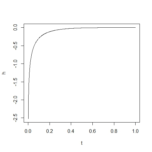
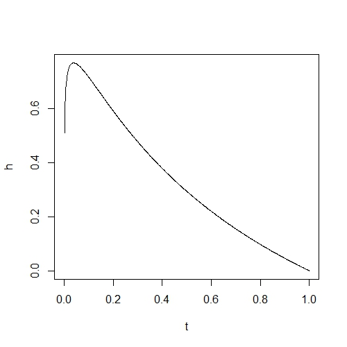
For illustration Figure 3.1 depicts the three cases of the lemma.

Refer to caption
(a)
Refer to caption
(b)
Refer to caption
(c)
Figure 3.1. Graphs of hh in different parameter regions. In all plots λ=0.3\lambda=0.3 is chosen. A) corresponds to point (1) in the lemma and the graph illustrates a=0.9>−6/13a=0.9>-6/13. B) corresponds to point (2) in the lemma and the graph illustrates a=−6/13a=-6/13. C) corresponds to point (3) in the lemma and the graph illustrates a=−0.9<−6/13a=-0.9<-6/13.
Proof.

The proof is a consequence of the from of the derivatives of hh.

  1. (1)

    The function tλ+t−λ​t1+λ​t−1\frac{t}{\lambda+t}-\frac{\lambda t}{1+\lambda t}-1 is increasing on [0,1][0,1] and achieves the maximum −2​λ1+λ-\frac{2\lambda}{1+\lambda} at t=1t=1. Hence, if a>−2​λ1+λa>\frac{-2\lambda}{1+\lambda} then h′​(t)=0h^{\prime}(t)=0 has no solution on (0,1](0,1] i.e. h′h^{\prime} is either positive or negative on the whole interval. Since h⁡(0)=−∞h(0)=-\infty and h⁡(1)=0h(1)=0 it follows that hh is strictly increasing on [0,1)[0,1) and subsequently we also have that h⁡(t)≤0h(t)\leq 0 on (0,1](0,1].

  2. (2)

    It holds that t±​(a=−2​λ1+λ)=1t_{\pm}\left(a=\frac{-2\lambda}{1+\lambda}\right)=1 and that h′​(1)=h′′​(1)=0h^{\prime}(1)=h^{\prime\prime}(1)=0 and h′′′​(1)=2​λ​(1−λ)(1+λ)3h^{\prime\prime\prime}(1)=\frac{2\lambda(1-\lambda)}{(1+\lambda)^{3}}. As in (1) we can conclude that t=1t=1 is the only zero of h′h^{\prime} in (0,1](0,1] so that h′h^{\prime} is strictly positive. Furthermore it holds that h⁡(t)≤0h(t)\leq 0 on (0,1](0,1].

  3. (3)

    If a∈(−1,−2​λ1+λ)a\in(-1,\,\frac{-2\lambda}{1+\lambda}) then t−∈(0,1)t_{-}\in(0,1) and t+>1t_{+}>1 so that h′h^{\prime} has a unique zero t−∈(0,1)t_{-}\in(0,1). Plugging this into our formula for h′′​(t)h^{\prime\prime}(t) we find that

    h′′​(t−)=λt−​(−1(λ+t−)2+1(1+λ​t−)2)<0.\displaystyle h^{\prime\prime}(t_{-})=\frac{\lambda}{t_{-}}\left(-\frac{1}{(\lambda+t_{-})^{2}}+\frac{1}{(1+\lambda t_{-})^{2}}\right)<0.

    We conclude that t−t_{-} is a local maximum of hh and that hh is decreasing in a neighborhood of t−t_{-}. Since limt→0+h⁡(t)=−∞\lim_{t\rightarrow 0+}h(t)=-\infty and h⁡(1)=0h(1)=0 and there are no other critical points of hh we conclude that h⁡(t−)h(t_{-}) is a global maximum of hh and therefore it is positive.

∎

We are ready to present the asymptotic behavior of the Laplace-type integral.

Proposition 5.

Let λ∈(0,1)\lambda\in(0,1), a>−1a>-1 and let α,β>−1\alpha,\ \beta>-1. We have the following asymptotic behavior as n→∞n\rightarrow\infty:

  1. (1)

    If a>−2​λ1+λa>\frac{-2\lambda}{1+\lambda} then

    ∫01(1+λ​t)β​tαt+λ​(t(a+1)​1+λ​tt+λ)n​𝑑t=1n​(1+λ)βλ⁡(a+2)+a​(1+𝒪⁡(1n)).\displaystyle\int_{0}^{1}\frac{(1+\lambda t)^{\beta}t^{\alpha}}{t+\lambda}\left(t^{(a+1)}\frac{1+\lambda t}{t+\lambda}\right)^{n}{\rm d}t=\frac{1}{n}\frac{(1+\lambda)^{\beta}}{\lambda(a+2)+a}\left(1+\mathcal{O}\left(\frac{1}{n}\right)\right).
  2. (2)

    If a=−2​λ1+λa=\frac{-2\lambda}{1+\lambda} then

    ∫01(1+λ​t)β​tαt+λ​(t(a+1)​1+λ​tt+λ)n​𝑑t=Γ⁡(1/3)32/3​n1/3​(1+λ)β(λ⁡(1−λ))1/3​(1+𝒪⁡(1n1/3)).\displaystyle\int_{0}^{1}\frac{(1+\lambda t)^{\beta}t^{\alpha}}{t+\lambda}\left(t^{(a+1)}\frac{1+\lambda t}{t+\lambda}\right)^{n}{\rm d}t=\frac{\Gamma(1/3)}{3^{2/3}n^{1/3}}\frac{(1+\lambda)^{\beta}}{\left(\lambda(1-\lambda)\right)^{1/3}}\left(1+\mathcal{O}\left(\frac{1}{n^{1/3}}\right)\right).
  3. (3)

    If a∈(−1,−2​λ1+λ)a\in(-1,\,\frac{-2\lambda}{1+\lambda}) then g⁡(t−)>1g(t_{-})>1 and

    ∫01(1+λ​t)β​tαt+λ​(t(a+1)​1+λ​tt+λ)n​𝑑t\displaystyle\int_{0}^{1}\frac{(1+\lambda t)^{\beta}t^{\alpha}}{t+\lambda}\left(t^{(a+1)}\frac{1+\lambda t}{t+\lambda}\right)^{n}{\rm d}t
    =(1+λ​t−)β+1​t−α​(g⁡(t−))n​2​π​t−n​λ​((1+λ​t−)2−(λ+t−)2)​(1+𝒪⁡(1n1/2)),\displaystyle=(1+\lambda t_{-})^{\beta+1}t_{-}^{\alpha}\left(g(t_{-})\right)^{n}\sqrt{\frac{2\pi t_{-}}{n\lambda\left((1+\lambda t_{-})^{2}-(\lambda+t_{-})^{2}\right)}}\left(1+\mathcal{O}\left(\frac{1}{n^{1/2}}\right)\right),

    where t−t_{-} is defined in Equation (3.1).

Proof.

For properties of hh we refer to the respective points of Lemma 4. We first rewrite our Laplace integral so that the assumptions in A. Erdélyi’s asymptotic formula [59, Theorem 7.1] are met:

∫01(1+λ​t)β​tαt+λ​(t(a+1)​1+λ​tt+λ)n​𝑑t\displaystyle\int_{0}^{1}\frac{(1+\lambda t)^{\beta}t^{\alpha}}{t+\lambda}\left(t^{(a+1)}\frac{1+\lambda t}{t+\lambda}\right)^{n}{\rm d}t =∫−10(1−λ​t)β​(−t)αλ−t​((−t)(a+1)​1−λ​tλ−t)n​𝑑t\displaystyle=\int_{-1}^{0}\frac{(1-\lambda t)^{\beta}(-t)^{\alpha}}{\lambda-t}\left((-t)^{(a+1)}\frac{1-\lambda t}{\lambda-t}\right)^{n}{\rm d}t
=∫−10f~​(t)​e−n​h~​(t)​𝑑t,\displaystyle=\int_{-1}^{0}\tilde{f}(t)e^{-n\tilde{h}(t)}{\rm d}t,

where

f~​(t)\displaystyle\tilde{f}(t) =f⁡(−t)=(1−λ​t)β​(−t)αλ−t,\displaystyle=f(-t)=\frac{(1-\lambda t)^{\beta}(-t)^{\alpha}}{\lambda-t},
h~​(t)\displaystyle\tilde{h}(t) =−h⁡(−t)=−ln⁡((−t)a+1​1−λ​tλ−t).\displaystyle=-h(-t)=-\ln\left((-t)^{a+1}\frac{1-\lambda t}{\lambda-t}\right).
  1. (1)

    If a>−2​λ1+λa>\frac{-2\lambda}{1+\lambda} then h~​(−1)=0\tilde{h}(-1)=0, limt→0+h~​(t)=+∞\lim_{t\rightarrow 0^{+}}\tilde{h}(t)=+\infty and for t∈[−1,0)t\in[-1,0) we have h~​(t)≥0\tilde{h}(t)\geq 0 and h~′​(t)>0\tilde{h}^{\prime}(t)>0. Applying Erdélyi’s result we get

    ∫−10f~​(t)​e−n​h~​(t)​𝑑t\displaystyle\int_{-1}^{0}\tilde{f}(t)e^{-n\tilde{h}(t)}{\rm d}t =f~​(−1)n​h~′​(−1)​en​h~​(−1)​(1+𝒪⁡(1n))\displaystyle=\frac{\tilde{f}(-1)}{n\tilde{h}^{\prime}(-1)}e^{n\tilde{h}(-1)}\left(1+\mathcal{O}\left(\frac{1}{n}\right)\right)
    =1n​(1+λ)βλ⁡(a+2)+a​(1+𝒪⁡(1n))\displaystyle=\frac{1}{n}\frac{(1+\lambda)^{\beta}}{\lambda(a+2)+a}\left(1+\mathcal{O}\left(\frac{1}{n}\right)\right)

    which completes the proof.

  2. (2)

    If a=−2​λ1+λa=-\frac{2\lambda}{1+\lambda} then h~\tilde{h} is positive and strictly increasing on [−1,0)[-1,0) with h~​(−1)=0\tilde{h}(-1)=0, limt→0−h~​(t)=∞\lim_{t\rightarrow 0^{-}}\tilde{h}(t)=\infty. Moreover h~′​(−1)=h~′′​(−1)=0\tilde{h}^{\prime}(-1)=\tilde{h}^{\prime\prime}(-1)=0 while h~(3)​(−1)=h(3)​(1)=2​λ​(1−λ)(1+λ)3>0\tilde{h}^{(3)}(-1)=h^{(3)}(1)=\frac{2\lambda(1-\lambda)}{(1+\lambda)^{3}}>0. Applying again Erdélyi’s result we get

    ∫−10f~​(t)​e−n​h~​(t)​𝑑t\displaystyle\int_{-1}^{0}\tilde{f}(t)e^{-n\tilde{h}(t)}{\rm d}t =f~​(−1)​e−n​h~​(−1)​Γ⁡(1/3)3​(3!n​h~(3)​(−1))1/3​(1+𝒪⁡(1n1/3))\displaystyle=\tilde{f}(-1)e^{-n\tilde{h}(-1)}\frac{\Gamma(1/3)}{3}\left(\frac{3!}{n\tilde{h}^{(3)}(-1)}\right)^{1/3}\left(1+\mathcal{O}\left(\frac{1}{n^{1/3}}\right)\right)
    =(1+λ)β−1n1/3​Γ⁡(1/3)32/3​1+λ(λ⁡(1−λ))1/3​(1+𝒪⁡(1n1/3))\displaystyle=\frac{(1+\lambda)^{\beta-1}}{n^{1/3}}\frac{\Gamma(1/3)}{3^{2/3}}\frac{1+\lambda}{\left(\lambda(1-\lambda)\right)^{1/3}}\left(1+\mathcal{O}\left(\frac{1}{n^{1/3}}\right)\right)
    =1n1/3​Γ⁡(1/3)32/3​(1+λ)β(λ⁡(1−λ))1/3​(1+𝒪⁡(1n1/3)).\displaystyle=\frac{1}{n^{1/3}}\frac{\Gamma(1/3)}{3^{2/3}}\frac{(1+\lambda)^{\beta}}{\left(\lambda(1-\lambda)\right)^{1/3}}\left(1+\mathcal{O}\left(\frac{1}{n^{1/3}}\right)\right).
  3. (3)

    If a∈(−1,−2​λ1+λ)a\in(-1,\,\frac{-2\lambda}{1+\lambda}) then t−t_{-} is the unique maximum of hh on (0,1)(0,1) with g⁡(t−)=eh⁡(t−)>1g(t_{-})=e^{h(t_{-})}>1. Applying a standard result [2, Formula (6.4.19c)] we obtain

    ∫01(1+λ​t)β​tαt+λ​(t(a+1)​1+λ​tt+λ)n​𝑑t\displaystyle\int_{0}^{1}\frac{(1+\lambda t)^{\beta}t^{\alpha}}{t+\lambda}\left(t^{(a+1)}\frac{1+\lambda t}{t+\lambda}\right)^{n}{\rm d}t
    =(1+λ​t−)β​t−αt−+λ​2​π−n​h′′​(t−)​(g⁡(t−))n​(1+𝒪⁡(1n1/2)).\displaystyle=\frac{(1+\lambda t_{-})^{\beta}t_{-}^{\alpha}}{t_{-}+\lambda}\sqrt{\frac{2\pi}{-nh^{\prime\prime}(t_{-})}}\left(g(t_{-})\right)^{n}\left(1+\mathcal{O}\left(\frac{1}{n^{1/2}}\right)\right).

    Moreover

    2​π−n​h′′​(t−)=(λ+t−)​(1+λ​t−)​2​π​t−n​λ​((1+λ​t−)2−(λ+t−)2)\displaystyle\sqrt{\frac{2\pi}{-nh^{\prime\prime}(t_{-})}}=(\lambda+t_{-})(1+\lambda t_{-})\sqrt{\frac{2\pi t_{-}}{n\lambda\left((1+\lambda t_{-})^{2}-(\lambda+t_{-})^{2}\right)}}

    and the result follows.

∎

4. Simple estimates in the exponential regions

For applications it is often useful to identify parameter regions of exponential decay and to have simple upper estimates in such cases. The accumulated contribution of those regions is usually asymptotically negligible with the dominant contribution arising from the asymptotically larger parameter regions. The following proposition contains a simple characteristics of parameter regions of exponential behavior.

Proposition 6.

Let α,β>−1\alpha,\ \beta>-1, a>−1a>-1, λ∈(0, 1)\lambda\in(0,\,1) and nn be a positive integer.

  1. (1)

    We assume that a​n+αan+\alpha is an integer.

    1. (a)

      If a>2​λ1−λa>\frac{2\lambda}{1-\lambda} then there is x∗∈(λ,1)x^{*}\in(\lambda,1) such that (x∗)a+1​1−λ​x∗x∗−λ∈(0, 1)\left(x^{*}\right)^{a+1}\frac{1-\lambda x^{*}}{x^{*}-\lambda}\in(0,\,1) and

      |λa​n+α​(1−λ2)β​Pn(a​n+α,β)​(1−2​λ2)|\displaystyle\left|\lambda^{an+\alpha}(1-\lambda^{2})^{\beta}P_{n}^{(an+\alpha,\,\beta)}(1-2\lambda^{2})\right|
      ≤(x∗)α+1​(1+λ​x∗)β+1(1−x∗​λ)​(x∗−λ)​((x∗)a+1​1−λ​x∗x∗−λ)n.\displaystyle\leq\left(x^{*}\right)^{\alpha+1}\frac{(1+\lambda x^{*})^{\beta+1}}{(1-x^{*}\lambda)(x^{*}-\lambda)}\left(\left(x^{*}\right)^{a+1}\frac{1-\lambda x^{*}}{x^{*}-\lambda}\right)^{n}.

      x∗x^{*} is computed explicitly below.

    2. (b)

      If −1<a<−2​λ1+λ-1<a<\frac{-2\lambda}{1+\lambda} then there is x∗∈(1,1/λ)x^{*}\in(1,1/\lambda) such that (x∗)a+1​1+λ​x∗x∗+λ∈(0,1)\left(x^{*}\right)^{a+1}\frac{1+\lambda x^{*}}{x^{*}+\lambda}\in(0,1) and

      |λa​n+α​(1−λ2)b​n+β​Pn(a​n+α,β)​(1−2​λ2)|\displaystyle\left|\lambda^{an+\alpha}(1-\lambda^{2})^{bn+\beta}P_{n}^{(an+\alpha,\,\beta)}(1-2\lambda^{2})\right|
      ≤(x∗)α+1​(1+λ​x∗)β+1(1−x∗​λ)​(x∗−λ)​((x∗)a+1​1+λ​x∗x∗+λ)n.\displaystyle\leq\left(x^{*}\right)^{\alpha+1}\frac{(1+\lambda x^{*})^{\beta+1}}{(1-x^{*}\lambda)(x^{*}-\lambda)}\left(\left(x^{*}\right)^{a+1}\frac{1+\lambda x^{*}}{x^{*}+\lambda}\right)^{n}.

      x∗x^{*} is computed explicitly below.

  2. (2)

    We assume that a​n+αan+\alpha is not an integer.

    1. (a)

      If a>2​λ1−λa>\frac{2\lambda}{1-\lambda} then there is x∗∈(0,1)x^{*}\in(0,1) such that (x∗)a+1​1−λ​x∗x∗−λ,(x∗)a+1​1+λ​x∗x∗+λ∈(0,1)\left(x^{*}\right)^{a+1}\frac{1-\lambda x^{*}}{x^{*}-\lambda},\left(x^{*}\right)^{a+1}\frac{1+\lambda x^{*}}{x^{*}+\lambda}\in(0,1) and

      |λa​n+α​(1−λ2)β​Pn(a​n+α,β)​(1−2​λ2)|\displaystyle|\lambda^{an+\alpha}(1-\lambda^{2})^{\beta}P_{n}^{(an+\alpha,\,\beta)}(1-2\lambda^{2})|
      ≤(x∗)α+1​(1+λ​x∗)β+1(1−x∗​λ)​(x∗−λ)\displaystyle\leq\left(x^{*}\right)^{\alpha+1}\frac{(1+\lambda x^{*})^{\beta+1}}{(1-x^{*}\lambda)(x^{*}-\lambda)}
      ⋅[((x∗)a+1​1−λ​x∗x∗−λ)n+((x∗)a+1​1+λ​x∗x∗+λ)n].\displaystyle\cdot\left[\left(\left(x^{*}\right)^{a+1}\frac{1-\lambda x^{*}}{x^{*}-\lambda}\right)^{n}+\left(\left(x^{*}\right)^{a+1}\frac{1+\lambda x^{*}}{x^{*}+\lambda}\right)^{n}\right].

      x∗x^{*} is computed explicitly below.

    2. (b)

      If a∈(−1,−2​λ1+λ)a\in(-1,-\frac{2\lambda}{1+\lambda}) and if the sequence (a​n+α)n(an+\alpha)_{n} is separate from integers then the quantity

      λa​n+α​Pn(a​n+α,β)​(1−2​λ2)\lambda^{an+\alpha}P_{n}^{(an+\alpha,\,\beta)}(1-2\lambda^{2})

      increases exponentially in magnitude. The precise behavior depends on the proximity of the sequence (a​n+α)n(an+\alpha)_{n} to integers, see the proof of Theorem 1 point (4).

Proof of Proposition 6, point 1.

Since a​n+αan+\alpha is assumed to be an integer it is sufficient to consider the Fourier integral. Clearly

|1π​ℜ⁡{∫0πzα+1​(1−λ​z)βz−λ​(za+1​1−λ​zz−λ)n|z=x​ei​φ​d​φ}|≤max|z|=x⁡(|zα+1​(1−λ​z)βz−λ|​|za+1​1−λ​zz−λ|n).\displaystyle\left|\frac{1}{\pi}\Re{\left\{\int_{0}^{\pi}z^{\alpha+1}\frac{(1-\lambda z)^{\beta}}{z-\lambda}\bigg(z^{a+1}\frac{1-\lambda z}{z-\lambda}\bigg)^{n}\Bigg|_{z=xe^{i\varphi}}\textnormal{d}\varphi\right\}}\right|\leq\max_{\left|z\right|=x}\left(\left|z^{\alpha+1}\frac{(1-\lambda z)^{\beta}}{z-\lambda}\right|\left|z^{a+1}\frac{1-\lambda z}{z-\lambda}\right|^{n}\right).

Recall that for z,w∈𝔻z,w\in\mathbb{D} it holds that [35, Formula (1.11)]

|z|−|w|1−|z|​|w|≤|z−w1−w¯​z|≤|z|+|w|1+|z|​|w|.\displaystyle\frac{|z|-|w|}{1-|z||w|}\leq\left|\frac{z-w}{1-\bar{w}z}\right|\leq\frac{|z|+|w|}{1+|z||w|}.

This implies that

max|z|=x⁡|za+1​1−λ​zz−λ|≤{xa+1​1−λ​xx−λ,x∈(λ,1]xa+1​1+λ​xx+λ,x∈(1,∞).\max_{|z|=x}\left|z^{a+1}\frac{1-\lambda z}{z-\lambda}\right|\leq\begin{cases}x^{a+1}\frac{1-\lambda x}{x-\lambda},\ x\in(\lambda,1]\\ x^{a+1}\frac{1+\lambda x}{x+\lambda},\ x\in(1,\infty)\end{cases}.
  1. (1)

    Suppose that a>2​λ1−λa>\frac{2\lambda}{1-\lambda}. The derivative of x↦xa+1​1−λ​xx−λx\mapsto x^{a+1}\frac{1-\lambda x}{x-\lambda} has zeros at

    x±=a+(a+2)​λ22​λ​(a+1)±(a+(a+2)​λ22​λ​(a+1))2−1.x_{\pm}=\frac{a+(a+2)\lambda^{2}}{2\lambda(a+1)}\pm\sqrt{\left(\frac{a+(a+2)\lambda^{2}}{2\lambda(a+1)}\right)^{2}-1}.

    Notice that x±​(a=2​λ1−λ)=1x_{\pm}(a=\frac{2\lambda}{1-\lambda})=1 and that x−​(a→∞)→λx_{-}(a\rightarrow\infty)\rightarrow\lambda, x+​(a→∞)→1/λx_{+}(a\rightarrow\infty)\rightarrow 1/\lambda. The function

    a↦y⁡(a)=a+(a+2)​λ22​λ​(a+1),a>−1a\mapsto y(a)=\frac{a+(a+2)\lambda^{2}}{2\lambda(a+1)},\ a>-1

    is increasing for λ∈(0,1)\lambda\in(0,1). The functions y↦y±y2−1y\mapsto y\pm\sqrt{y^{2}-1} are, respectively, increasing/ decreasing for y>1y>1. It follows that x−​(a)x_{-}(a) is decreasing and x+​(a)x_{+}(a) is increasing for a>2​λ1−λa>\frac{2\lambda}{1-\lambda}. Consequently x−∈(λ,1)x_{-}\in(\lambda,1) and x+∈(1,1/λ)x_{+}\in(1,1/\lambda). Choose x∗=x−x^{*}=x_{-} and notice that the second derivative of x↦xa+1​1−λ​xx−λx\mapsto x^{a+1}\frac{1-\lambda x}{x-\lambda} is strictly positive at x∗x^{*}; Moreover limx→λ+xa+1​1−λ​xx−λ=+∞\lim_{x\rightarrow\lambda^{+}}x^{a+1}\frac{1-\lambda x}{x-\lambda}=+\infty and xa+1​1−λ​xx−λ|x=1=1x^{a+1}\frac{1-\lambda x}{x-\lambda}\Big|_{x=1}=1. Taken together these properties are only possible if (x∗)a+1​1−λ​x∗x∗−λ<1\left(x^{*}\right)^{a+1}\frac{1-\lambda x^{*}}{x^{*}-\lambda}<1.

  2. (2)

    Suppose that a<−2​λ1+λa<-\frac{2\lambda}{1+\lambda}. The derivative of x↦xa+1​1+λ​xx+λx\mapsto x^{a+1}\frac{1+\lambda x}{x+\lambda} has zeros at

    x±=−a+(a+2)​λ22​λ​(a+1)±(a+(a+2)​λ22​λ​(a+1))2−1.x_{\pm}=-\frac{a+(a+2)\lambda^{2}}{2\lambda(a+1)}\pm\sqrt{\left(\frac{a+(a+2)\lambda^{2}}{2\lambda(a+1)}\right)^{2}-1}.

    Notice that x±​(a=−2​λ1+λ)=1x_{\pm}(a=-\frac{2\lambda}{1+\lambda})=1 and that x−​(a→−1)→0x_{-}(a\rightarrow-1)\rightarrow 0, x+​(a→−1)→∞x_{+}(a\rightarrow-1)\rightarrow\infty. The function

    a↦y⁡(a)=a+(a+2)​λ22​λ​(a+1),a>−1a\mapsto y(a)=\frac{a+(a+2)\lambda^{2}}{2\lambda(a+1)},\ a>-1

    is increasing for λ∈(0,1)\lambda\in(0,1). The functions y↦−y±y2−1y\mapsto-y\pm\sqrt{y^{2}-1} are, respectively, decreasing/ increasing for y<−1y<-1. It follows that x−​(a)x_{-}(a) is increasing and x+​(a)x_{+}(a) is decreasing on (−1,−2​λ1+λ)(-1,-\frac{2\lambda}{1+\lambda}). Consequently x−∈(0,1)x_{-}\in(0,1) and x+∈(1,∞)x_{+}\in(1,\infty). Fix ϵ>0\epsilon>0, choose x∗=min⁡{x+,1/λ−ϵ}x^{*}=\min\{x_{+},1/\lambda-\epsilon\} and notice that the second derivative of x↦xa+1​1+λ​xx+λx\mapsto x^{a+1}\frac{1+\lambda x}{x+\lambda} is strictly positive at x+x_{+}; Moreover limx→∞xa+1​1+λ​xx+λ=+∞\lim_{x\rightarrow\infty}x^{a+1}\frac{1+\lambda x}{x+\lambda}=+\infty and xa+1​1+λ​xx+λ|x=1=1x^{a+1}\frac{1+\lambda x}{x+\lambda}\Big|_{x=1}=1. Taken together these properties are only possible if (x∗)a+1​1+λ​x∗x∗+λ<1\left(x^{*}\right)^{a+1}\frac{1+\lambda x^{*}}{x^{*}+\lambda}<1.

∎

Proof of Proposition 6, point 2.

Since a​n+αan+\alpha is not an integer both the Fourier and the Laplace integral contribute. The generalized Fourier integral is estimated above.

  1. (1)

    Suppose that a>2​λ1−λa>\frac{2\lambda}{1-\lambda}. By Lemma 4, point (1), the function g:t↦t(a+1)​1+λ​tt+λg:\>t\mapsto t^{(a+1)}\frac{1+\lambda t}{t+\lambda} is strictly increasing on (0,1](0,1] and g⁡(t)≤1g(t)\leq 1 for t∈(0,1]t\in(0,1]. Consequently, with x∗x^{*} chosen as in the proof of Proposition 6, point (1a), it holds that (x∗)a+1​1+λ​x∗x∗+λ<1\left(x^{*}\right)^{a+1}\frac{1+\lambda x^{*}}{x^{*}+\lambda}<1. It follows that

    ∫0x∗(1+λ​t)β​tαt+λ​(ta+1​1+λ​tt+λ)n​𝑑t≤(x∗)α+1​(1+λ​x∗)β+1(x∗−λ)​(1−λ​x∗)​((x∗)a+1​1+λ​x∗x∗+λ)n\displaystyle\int_{0}^{x^{*}}\frac{(1+\lambda t)^{\beta}t^{\alpha}}{t+\lambda}\left(t^{a+1}\frac{1+\lambda t}{t+\lambda}\right)^{n}{\rm d}t\leq\frac{(x^{*})^{\alpha+1}(1+\lambda x^{*})^{\beta+1}}{(x^{*}-\lambda)(1-\lambda x^{*})}\left(\left(x^{*}\right)^{a+1}\frac{1+\lambda x^{*}}{x^{*}+\lambda}\right)^{n}

    which, combined with the estimate for the generalized Fourier integral, proves (2).

  2. (2)

    Suppose that −1<a<−2λ/(1+λ)-1<a<-2\lambda/(1+\lambda). Choose x∗x^{*} as in the proof of Proposition 6, point (1b). By Proposition 5, point 3, and the same reasoning as in (a) the Laplace integral increases exponentially in magnitude. At the same time the Fourier integral decays exponentially. This proves the assertion in case the sequence (a​n+α)n(an+\alpha)_{n} is separate from integers. In general we refer to formula (5.2), see the proof of Theorem 1 point 4) below.

∎

5. Proof of Theorem 1 and Comments

By Lemma 2 the asymptotic behavior of the JPVFPs can be obtained as a sum of the asymptotic formulas for the Fourier and Laplace-type integrals. Depending on the region of parameters either the one or the other (or both) provide the leading order contribution, which results in the diverse asymptotic behavior in regions 1)-4). It should be noticed that it is still a delicate question, which summand in the expansion of the JPVFPs actually provides the dominating contribution. Consider for instance the first order term in point 1),

(5.1) 2n​π​cos⁡(((n+1)​h​(φ+)+(α−a)​φ++(β−1)​ψ+π4)CLOSE,\displaystyle\sqrt{\frac{2}{n\pi}}\cos\left(((n+1)h(\varphi_{+})+(\alpha-a)\varphi_{+}+(\beta-1)\psi{+}\frac{\pi}{4}\right),

which is clearly 𝒪⁡(1/n1/2)\mathcal{O}(1/n^{1/2}), while the next term is 𝒪⁡(1/n3/2)\mathcal{O}(1/n^{3/2}). It is, in principle, possible that a subsequence exists such that the above is even 𝒪⁡(1/n1/2)\mathcal{O}(1/n^{1/2}). We illustrate this phenomenon with a brief lemma.

Lemma 7.

Let γ>0\gamma>0 be fixed. There exists a sequence sns_{n} of natural numbers so that |cos⁡(γ​sn+π2)|≤Ksn|\cos(\gamma s_{n}+\frac{\pi}{2})|\leq\frac{K}{s_{n}}.

Proof of Lemma 7.

We show that the sequence an=n​cos⁡(γ​n+π2)a_{n}=n\cos(\gamma n+\frac{\pi}{2}) has a convergent subsequence. Fix arbitrary nn and let, by Dirichlet’s theorem on Diophantine approximation, pn,qn∈ℕp_{n},q_{n}\in\mathbb{N} be chosen so that

|qn​πγ−pn|<1n,qn≤n.\displaystyle\left|q_{n}\frac{\pi}{\gamma}-p_{n}\right|<\frac{1}{n},\quad q_{n}\leq n.

The subsequence apna_{p_{n}} is bounded because

|apn|=|pn​cos⁡(γ​pn+π2)|=pn​|sin⁡(γ​pn−qn​π)|≤(n​πγ+1n)​γn≤π+γ.\displaystyle|a_{p_{n}}|=\left|p_{n}\cos(\gamma p_{n}+\frac{\pi}{2})\right|=p_{n}\left|\sin\left(\gamma p_{n}-q_{n}\pi\right)\right|\leq\left(n\frac{\pi}{\gamma}+\frac{1}{n}\right)\frac{\gamma}{n}\leq\pi+\gamma.

By the Bolzano-Weierstrass theorem apna_{p_{n}} has a convergent subsequence asna_{s_{n}}. ∎

Proof of Theorem 1.
  1. (1)

    Suppose a∈(−2​λ1+λ,2​λ1−λ)a\in(-\frac{2\lambda}{1+\lambda},\,\frac{2\lambda}{1-\lambda}) and choose x=1x=1 in Lemma 2. Comparing the second order term of the generalized Fourier integral in Proposition 3, point (1) to the first order term of the Laplace integral in Proposition 5, point (1), we observe an exact cancellation. We are therefore left with the first order term of the generalized Fourier integral, which is proportional to (5.1) and an additional contribution of 𝒪⁡(1/n3/2)\mathcal{O}(1/n^{3/2}).

  2. (2)

    Suppose a=2​λ1−λa=\frac{2\lambda}{1-\lambda} and choose x=1x=1 in Lemma 2. By Proposition 5, point (1), the contribution of the Laplace-type integral for a>−2​λ1+λa>-\frac{2\lambda}{1+\lambda} is 𝒪⁡(1/n)\mathcal{O}(1/n). By Proposition 3, point (2), the leading contribution to the generalized Fourier integral is Θ⁡(1/n1/3)\Theta(1/n^{1/3}). As a consequence only the Fourier integral determines the leading order behavior in this region. Suppose a=−2​λ1+λa=-\frac{2\lambda}{1+\lambda} and choose x=1x=1 in Lemma 2. By Proposition 5, point (2), and by Proposition 3, point (2), both integrals are of order 𝒪⁡(1/n1/3)\mathcal{O}(1/n^{1/3}). Summing the contributions according to Lemma 2 yields the formula claimed in the theorem.

  3. (3)

    If a​n+αan+\alpha is an integer then the Laplace-type integral does not contribute. The exponential decay of the Fourier-type integral in the region a∈(−1,−2​λ1+λ)∪(2​λ1−λ,∞)a\in(-1,\frac{-2\lambda}{1+\lambda})\cup(\frac{2\lambda}{1-\lambda},\infty) has been demonstrated as part of Proposition 6, which proves the statement of the theorem. For completeness let us mention that an application of the well-established saddle point method [83, Chapter II] to the Fourier-type integral yields

    λa​n+α​(1−λ2)β​Pn(a​n+α,β)​(1−2​λ2)\displaystyle\lambda^{an+\alpha}(1-\lambda^{2})^{\beta}P_{n}^{(an+\alpha,\,\beta)}(1-2\lambda^{2})
    =12​n​π​(a+1)​1Δ1/4​z−α+1​(1−λ​z−)βz−−λ​(z−a+1​(1−λ​z−)z−−λ)n​(1+𝒪⁡(1n1/2)),\displaystyle=\sqrt{\frac{1}{2n\pi(a+1)}}\frac{1}{\Delta^{1/4}}\frac{z_{-}^{\alpha+1}(1-\lambda z_{-})^{\beta}}{z_{-}-\lambda}\left(\frac{z_{-}^{a+1}(1-\lambda z_{-})}{z_{-}-\lambda}\right)^{n}\left(1+\mathcal{O}\left(\frac{1}{n^{1/2}}\right)\right),

    where

    Δ=(a+2​λ1+λ)​(a−2​λ1−λ),\Delta=\left(a+\frac{2\lambda}{1+\lambda}\right)\left(a-\frac{2\lambda}{1-\lambda}\right),
    z−=a+a​λ2+2​λ22​λ​(a+1)−(a+a​λ2+2​λ22​λ​(a+1))2−1,z_{-}=\frac{a+a\lambda^{2}+2\lambda^{2}}{2\lambda(a+1)}-\sqrt{\left(\frac{a+a\lambda^{2}+2\lambda^{2}}{2\lambda(a+1)}\right)^{2}-1},

    and |z−a+1​(1−λ​z−)z−−λ|<1\left|\frac{z_{-}^{a+1}(1-\lambda z_{-})}{z_{-}-\lambda}\right|<1. This is a verbatim adaptation of [17, Theorem 1, (2) and (4)].

  4. (4)

    If a​n+αan+\alpha is not an integer then the Laplace-type integral does contribute. If a>2​λ1−λa>\frac{2\lambda}{1-\lambda} it can be checked that the Laplace integral decays faster than the Fourier integral and the above formula remains valid. For a∈(−1,−2​λ1+λ)a\in(-1,\frac{-2\lambda}{1+\lambda}) the Laplace integral grows exponentially, while the Fourier integral decays exponentially, which proves the statement of the theorem. For completeness let us mention that Proposition 5, point 3) entails that

    (5.2) λa​n+α​(1−λ2)β​Pn(a​n+α,β)​(1−2​λ2)\displaystyle\lambda^{an+\alpha}(1-\lambda^{2})^{\beta}P_{n}^{(an+\alpha,\,\beta)}(1-2\lambda^{2})
    =−sin⁡(π⁡(a​n+α))π​(1+λ​t−)β+1​t−α​(g⁡(t−))n​2​π​t−n​λ​((1+λ​t−)2−(λ+t−)2)\displaystyle=-\frac{{\sin\left(\pi(an+\alpha)\right)}}{\pi}(1+\lambda t_{-})^{\beta+1}t_{-}^{\alpha}\left(g(t_{-})\right)^{n}\sqrt{\frac{2\pi t_{-}}{n\lambda\left((1+\lambda t_{-})^{2}-(\lambda+t_{-})^{2}\right)}}
    +𝒪⁡((g⁡(t−))nn),\displaystyle+\mathcal{O}\left(\frac{(g(t_{-}))^{n}}{n}\right),

    where t−t_{-} is given in (3.1), g⁡(t−)>1g(t_{-})>1. The precise asymptotic behavior of this quantity depends on the specific subsequence of natural numbers, as the proximity of this subsequence to the zeros of the sine term potentially tempers the rate of growth.

∎

6. Numerical experiments

We illustrate the findings of our main Theorem 1 with numerical plots in the respective parameter regions. In all cases the numerical experiments are consistent with the theoretical work. Results were obtained in MAPLE2020 and using the NumPy and Matplotlib packages of Python.

Figure 6.1 illustrates Theorem 1, point (1). JPFVPs of varying degree nn are evaluated numerically and compared to our approximation for two sets of parameters.

Figure 6.2 illustrates Theorem 1, point (2) at the right boundary, a=2​λ/(1−λ)a=2\lambda/(1-\lambda).

Figure 6.3 illustrates Theorem 1, point (2) at the left boundary, a=−2λ/(1+λ)a=-2\lambda/(1+\lambda).

Figure 6.4 illustrates the exponential region a∈(−1,−2​λ1+λ)∪(2​λ1−λ,∞)a\in(-1,\frac{-2\lambda}{1+\lambda})\cup(\frac{2\lambda}{1-\lambda},\infty) of Theorem 1, point (3). For two sets of parameters the JPFVPs are evaluated and displayed on a subsequence of degrees, where a​n+αan+\alpha is an integer.

Figure 6.5 illustrates the exponential region a∈(−1,−2​λ1+λ)∪(2​λ1−λ,∞)a\in(-1,\frac{-2\lambda}{1+\lambda})\cup(\frac{2\lambda}{1-\lambda},\infty) of Theorem 1, point (4). For three sets of parameters the JPFVPs are evaluated and displayed on a subsequence of degrees, where a​n+αan+\alpha is not an integer. In accordance with the claim of the theorem exponential decay is observed if a>2​λ1−λa>\frac{2\lambda}{1-\lambda}. However if a<−2​λ1+λa<\frac{-2\lambda}{1+\lambda} the JPFVPs show exponential growth.

Refer to caption
(a) λ=14\lambda=\frac{1}{4}, a=0.1a=0.1, α=β=0\alpha=\beta=0
Refer to caption
(b) λ=12\lambda=\frac{1}{2}, a=1a=1, α=β=0\alpha=\beta=0
Figure 6.1. Illustration of Theorem 1, point (1). Numerical computation of nn-dependence of JPVFPs and approximation for two sets of parameters.
Refer to caption
(a) λ=14\lambda=\frac{1}{4}, a=23a=\frac{2}{3}, α=β=0\alpha=\beta=0
Refer to caption
(b) λ=12\lambda=\frac{1}{2}, a=2a=2, α=β=0\alpha=\beta=0
Figure 6.2. Illustration of Theorem 1, point (2). Numerical computation of nn-dependence of JPVFPs and approximation at the right boundary. In case of the approximation only every 10th data point is displayed.
Refer to caption
(a) λ=14\lambda=\frac{1}{4}, a=−25a=-\frac{2}{5}, α=β=0\alpha=\beta=0
Refer to caption
(b) λ=12\lambda=\frac{1}{2}, a=−23a=-\frac{2}{3}, α=β=0\alpha=\beta=0
Figure 6.3. Illustration of Theorem 1, point (2). Numerical computation of nn-dependence of JPVFPs and approximation at the left boundary. In case of the approximation only every 4th data point is displayed.
Refer to caption
(a) λ=14\lambda=\frac{1}{4}, a=45>23a=\frac{4}{5}>\frac{2}{3}, α=β=0\alpha=\beta=0
Refer to caption
(b) λ=14\lambda=\frac{1}{4}, a=−12<−25a=-\frac{1}{2}<-\frac{2}{5}, α=β=0\alpha=\beta=0
Figure 6.4. Illustration of Theorem 1, point (3). Numerical computation of nn-dependence of JPVFPs and approximation in the exponential region. Data points are displayed only for such nn that a​n+αan+\alpha is an integer.
Refer to caption
(a) λ=14\lambda=\frac{1}{4}, a=45>23a=\frac{4}{5}>\frac{2}{3}, α=β=0\alpha=\beta=0
Refer to caption
(b) λ=14\lambda=\frac{1}{4}, a=−12<−25a=-\frac{1}{2}<-\frac{2}{5}, α=β=0\alpha=\beta=0
Refer to caption
(c) λ=12\lambda=\frac{1}{2}, a=−π4<−23a=-\frac{\pi}{4}<-\frac{2}{3}, α=β=0\alpha=\beta=0
Figure 6.5. Illustration of Theorem 1, point (4). Numerical computation of nn-dependence of JPVFPs and approximation in the exponential region. Data points are displayed only for such nn that a​n+αan+\alpha is not an integer.

7. Extensions

This section illustrates two possible extensions of our work.

7.1. Jacobi polynomials with varying parameters

The proof of Lemma 2 can be adapted to the more general JPVPs by integrating the function

f:z↦z(a+1)​n+α​(1−λ​z)(b+1)​n+β(z−λ)n+1f:z\mapsto z^{(a+1)n+\alpha}\frac{(1-\lambda z)^{(b+1)n+\beta}}{(z-\lambda)^{n+1}}

along the same contour as in Lemma 2. One easily obtains an integral representation for the JPVPs of the form

λa​n+α​(1−λ2)b​n+β​Pn(a​n+α,b​n+β)​(1−2​λ2)\displaystyle\lambda^{an+\alpha}(1-\lambda^{2})^{bn+\beta}P_{n}^{(an+\alpha,\,bn+\beta)}(1-2\lambda^{2})
=1π​ℜ⁡{∫0πzα+1​(1−λ​z)βz−λ​(za+1​(1−λ​z)b+1z−λ)n|z=x​ei​φ​d​φ}\displaystyle=\frac{1}{\pi}\Re\left\{\int_{0}^{\pi}{z^{\alpha+1}\frac{(1-\lambda z)^{\beta}}{z-\lambda}\bigg(z^{a+1}\frac{(1-\lambda z)^{b+1}}{z-\lambda}\bigg)^{n}}\Bigg|_{z={x}e^{i\varphi}}\textnormal{d}\varphi\right\}
−sin⁡(π⁡(α+a​n))π∫0x(1+λ​t)β​tαt+λ(t(a+1)(1+λ​t)b+1t+λ)ndt,\displaystyle-\frac{{\sin\left(\pi(\alpha+an)\right)}}{\pi}\int_{0}^{{x}}\frac{(1+\lambda t)^{\beta}t^{\alpha}}{t+\lambda}\left(t^{(a+1)}\frac{(1+\lambda t)^{b+1}}{t+\lambda}\right)^{n}{\rm d}t,

where x∈(λ, 1/λ)x\in(\lambda,\,1/\lambda). It should be mentioned that in this case the asymptotic analysis of the first integral is significantly more involved. Some asymptotic formulas can be obtained by applying the method of steepest descent along the lines of [83, Section 2], [5, Chapter 7]. This leads to the cases

  1. (1)

    a∈((1−λ​b+1)21−λ2−1,(1+λ​b+1)21−λ2−1)a\in\left(\frac{(1-\lambda\sqrt{b+1})^{2}}{1-\lambda^{2}}-1,\,\frac{(1+\lambda\sqrt{b+1})^{2}}{1-\lambda^{2}}-1\right),

  2. (2)

    a∈{(1−λ​b+1)21−λ2−1,(1+λ​b+1)21−λ2−1},a\in\left\{\frac{(1-\lambda\sqrt{b+1})^{2}}{1-\lambda^{2}}-1,\,\frac{(1+\lambda\sqrt{b+1})^{2}}{1-\lambda^{2}}-1\right\},

  3. (3)

    a∈((1+λ​b+1)21−λ2−1,∞),a\in\left(\frac{(1+\lambda\sqrt{b+1})^{2}}{1-\lambda^{2}}-1,\,\infty\right),

  4. (4)

    a∈(−1,(1−λ​b+1)21−λ2−1)a\in\left(-1,\,\frac{(1-\lambda\sqrt{b+1})^{2}}{1-\lambda^{2}}-1\right) and a​n+αan+\alpha is an integer,

  5. (5)

    a∈(−1,(1−λ​b+1)21−λ2−1)a\in\left(-1,\,\frac{(1-\lambda\sqrt{b+1})^{2}}{1-\lambda^{2}}-1\right) and a​n+αan+\alpha is not an integer.

For instance if a∈((1−λ​b+1)21−λ2−1,(1+λ​b+1)21−λ2−1)a\in\left(\frac{(1-\lambda\sqrt{b+1})^{2}}{1-\lambda^{2}}-1,\,\frac{(1+\lambda\sqrt{b+1})^{2}}{1-\lambda^{2}}-1\right) then

λa​n+α​(1−λ2)b​n+β​Pn(a​n+α,b​n+β)​(1−2​λ2)=\displaystyle\lambda^{an+\alpha}(1-\lambda^{2})^{bn+\beta}P_{n}^{(an+\alpha,\,bn+\beta)}(1-2\lambda^{2})=
2n​πℜ{(G(z+)(z+2iH′′(z+))−1/2)en​H​(z+)+i​π4}(1+𝒪(1n1/2)),\displaystyle\sqrt{\frac{2}{n\pi}}\Re\left\{\left(G(z_{+})\left(z_{+}^{2}iH^{\prime\prime}(z_{+})\right)^{-1/2}\right)e^{nH(z_{+})+i\frac{\pi}{4}}\right\}\left(1+\mathcal{O}\left(\frac{1}{n^{1/2}}\right)\right),

where

G⁡(z)=zα+1​(1−λ​z)βz−λ,H⁡(z)=Log⁡(za+1​(1−λ​z)b+1z−λ)G(z)=\frac{z^{\alpha+1}(1-\lambda z)^{\beta}}{z-\lambda},\qquad H(z)=\Log\left(\frac{z^{a+1}(1-\lambda z)^{b+1}}{z-\lambda}\right)

and

z±=λ2​(a+b+2)+a2​λ​(a+b+1)±(λ2​(a+b+2)+a2​λ​(a+b+1))2−a+1a+b+1z_{\pm}=\frac{\lambda^{2}(a+b+2)+a}{2\lambda(a+b+1)}\pm\sqrt{\left(\frac{\lambda^{2}(a+b+2)+a}{2\lambda(a+b+1)}\right)^{2}-\frac{a+1}{a+b+1}}

satisfy H′​(z±)=0H^{\prime}(z_{\pm})=0 and H′′​(z±)≠0H^{\prime\prime}(z_{\pm})\neq 0, which generalizes Theorem 1 point (1). This formula coincides with [32, Proposition 6.1]. Similar to Theorem 1, point 3), if a∈((1+λ​b+1)21−λ2−1,∞)a\in\left(\frac{(1+\lambda\sqrt{b+1})^{2}}{1-\lambda^{2}}-1,\,\infty\right) and a+b+1>0a+b+1>0 then the Laplace-type integral does not contribute, leading to

λa​n+α​(1−λ2)b​n+β​Pn(a​n+α,b​n+β)​(1−2​λ2)\displaystyle\lambda^{an+\alpha}(1-\lambda^{2})^{bn+\beta}P_{n}^{(an+\alpha,\,bn+\beta)}(1-2\lambda^{2})
=12​n​π​H′′​(z−)​G⁡(z−)z−​(z−a+1​(1−λ​z−)b+1z−−λ)n​(1+𝒪⁡(1n1/2)).\displaystyle=\sqrt{\frac{1}{2n\pi H^{\prime\prime}(z_{-})}}\frac{G(z_{-})}{z_{-}}\left(\frac{z_{-}^{a+1}(1-\lambda z_{-})^{b+1}}{z_{-}-\lambda}\right)^{n}\left(1+\mathcal{O}\left(\frac{1}{n^{1/2}}\right)\right).

However, if a∈(−1,(1−λ​b+1)21−λ2−1)a\in\left(-1,\,\frac{(1-\lambda\sqrt{b+1})^{2}}{1-\lambda^{2}}-1\right) the condition that a​n+αan+\alpha is an integer plays a similar role as for b=0b=0. If a∈(−1,(1−λ​b+1)21−λ2−1)a\in\left(-1,\,\frac{(1-\lambda\sqrt{b+1})^{2}}{1-\lambda^{2}}-1\right), a+b+1>0a+b+1>0 and a​n+αan+\alpha is an integer then

λa​n+α​(1−λ2)b​n+β​Pn(a​n+α,b​n+β)​(1−2​λ2)\displaystyle\lambda^{an+\alpha}(1-\lambda^{2})^{bn+\beta}P_{n}^{(an+\alpha,\,bn+\beta)}(1-2\lambda^{2})
=−12​n​π​H′′​(z−)​z−(a+1)​n+α​(1−λ​z−)(b+1)​n+β(z−−λ)n+1​(1+𝒪⁡(1n1/2)).\displaystyle=-\sqrt{\frac{1}{2n\pi H^{\prime\prime}(z_{-})}}\frac{z_{-}^{(a+1)n+\alpha}(1-\lambda z_{-})^{(b+1)n+\beta}}{(z_{-}-\lambda)^{n+1}}\left(1+\mathcal{O}\left(\frac{1}{n^{1/2}}\right)\right).

7.2. Uniform asymptotic expansions

The theory of uniform asymptotic expansions is concerned with asymptotic expansions that hold when a parameter varies throughout different ranges of asymptotic behavior. We describe briefly the methodology to obtain uniform expansions for JPVFPs when aa passes over the critical boundaries {−2​λ1+λ,2​λ1−λ}\{-\frac{2\lambda}{1+\lambda},\frac{2\lambda}{1-\lambda}\}. Luckily even in this situation standard tools are available [11, Section 2.3], [5, Section 9.2], [83, p. 366–372], which are all based on the so-called uniform method of steepest decent [26]. For brevity consider the Fourier integral, see Section 3.1. When aa approaches the boundary, the radius of convergence of the asymptotic expansion goes to 00. Indeed when aa varies in ℝ∖{−2​λ1+λ,2​λ1−λ}\mathbb{R}\setminus\{-\frac{2\lambda}{1+\lambda},\frac{2\lambda}{1-\lambda}\} the saddle points z±z_{\pm} of hah_{a} are of order one, but when aa approaches the critical boundary z±z_{\pm} coalesce to saddle points of order 22. If aa approaches the boundary from the inside the two saddle points z±z_{\pm} remain on the unit circle ∂𝔻\partial\mathbb{D}. But if aa approaches the boundary from the outside the saddle points z±z_{\pm} move along the real line. While in the former situation z±z_{\pm} automatically lie on the contour of integration, in the latter case the contour of integration is deformed such that the new contour passes through the saddle points z±z_{\pm} and 11. To simplify the dependence of z±z_{\pm} on aa a change of variable is applied via a locally one-to-one transformation. This is made precise in the below proposition, where (overriding previous notation)

f⁡(z)=fa​(z)=Log⁡(za+1​(1−λ​z)z−λ).f(z)=f_{a}(z)={\rm Log}\left(\frac{z^{a+1}(1-\lambda z)}{z-\lambda}\right).
Proposition 8 ([74, Proposition 16]).

For aa in a small neighborhood of 2​λ1−λ\frac{2\lambda}{1-\lambda} the cubic transformation

fa​(z)=−t33+γ2​tf_{a}(z)=-\frac{t^{3}}{3}+\gamma^{2}t

with

γ2=(a−2​λ1−λ)​(1−λ)(λ⁡(1+λ))1/3+𝒪⁡(a−2​λ1−λ),\gamma^{2}=\frac{(a-\frac{2\lambda}{1-\lambda})(1-\lambda)}{\left(\lambda(1+\lambda)\right)^{1/3}}+{\scriptstyle\mathcal{O}}\left(a-\frac{2\lambda}{1-\lambda}\right),

has exactly one branch t=t⁡(z,a)t=t(z,a) that can be expanded into a power series in zz with coefficients that are continuous in aa. On this branch the points z=z±z=z_{\pm} correspond to t=±γt=\pm\gamma. The mapping of zz to tt is one-to-one on a small neighborhood of z=1z=1 containing z+z_{+} and z−z_{-}.

This is an immediate corollary of [26]. A proof can be found in the appendix of [77]. To determine the asymptotics of the Fourier integral over a new suitable contour 𝒞\mathcal{C} we apply the transformation to a neighborhood of z0=1z_{0}=1. This yields a uniform expansion of the integral in terms of the Airy function A​iAi. For real arguments the latter can be defined as

A​i​(x)=1π​∫0∞cos⁡(t33+x​t)​d​t.Ai(x)=\frac{1}{\pi}\int_{0}^{\infty}\cos\left(\frac{t^{3}}{3}+xt\right)\textnormal{d}t.

For large negative arguments the Airy function shows oscillatory behavior

A​i​(−x)=1x1/4​π​(cos⁡(23​x3/2−π4)+𝒪⁡(1)),x→+∞,Ai(-x)=\frac{1}{x^{1/4}\sqrt{\pi}}\left(\cos\left(\frac{2}{3}x^{3/2}-\frac{\pi}{4}\right)+{\scriptstyle\mathcal{O}}(1)\right),\qquad x\rightarrow+\infty,
A​i′​(−x)=x1/4π​(sin⁡(23​x3/2−π4)+𝒪⁡(1)),x→+∞,Ai^{\prime}(-x)=\frac{x^{1/4}}{\sqrt{\pi}}\left(\sin\left(\frac{2}{3}x^{3/2}-\frac{\pi}{4}\right)+{\scriptstyle\mathcal{O}}(1)\right),\qquad x\rightarrow+\infty,

and exponential behavior for large positive arguments

A​i​(x)∼12​x1/4​π​exp⁡(−23​x3/2),A​i′​(x)∼−x1/42​π​exp⁡(−23​x3/2),x→+∞.Ai(x)\sim\frac{1}{2x^{1/4}\sqrt{\pi}}\exp\left(-\frac{2}{3}x^{3/2}\right),\ Ai^{\prime}(x)\sim-\frac{x^{1/4}}{2\sqrt{\pi}}\exp\left(-\frac{2}{3}x^{3/2}\right),\ x\rightarrow+\infty.

Following the procedure described in [5, p. 371–375] yields an asymptotic expansion of ∫∂𝔻g⁡(z)​en​f​(z)​d​zz\int_{\partial\mathbb{D}}g(z)e^{nf(z)}\frac{\textnormal{d}z}{z} for aa in a neighborhood of 2​λ1−λ\frac{2\lambda}{1-\lambda} in terms of A​iAi and A​i′Ai^{\prime}. Finally, if a​n+αan+\alpha is not an integer the Laplace integral must be taken into account. In this case [26] can be applied to t↦log⁡(t(a+1)​1+λ​tt+λ)t\mapsto\log\left(t^{(a+1)}\frac{1+\lambda t}{t+\lambda}\right), since as aa approaches a0,a_{0}, its critical points

t±=−λ2​(a+2)+a2​λ​(a+1)±(λ2​(a+2)+a2​λ​(a+1))2−1,t_{\pm}=-\frac{\lambda^{2}(a+2)+a}{2\lambda(a+1)}\pm\sqrt{\left(\frac{\lambda^{2}(a+2)+a}{2\lambda(a+1)}\right)^{2}-1},

coalesce to t0=1.t_{0}=1.

References

  • [2] C. M. Bender, S. A. Orszag, Advanced mathematical methods for Scientists and Engineers I: Asymptotic methods and perturbation theory, Volume 1. Springer, (1978).
  • [5] N. Bleistein, R. A. Handelsman, Asymptotic Expansions of Integrals, Dover Publications, Inc., New York, 2nd edition, (1986).
  • [8] M. Y. Blyudze, S. M. Shimorin, Estimates of the norms of powers of functions in certain Banach space, J. Math. Sci. 80:4, 1880–1891, (1996).
  • [11] V. A. Borovikov, Uniform Stationary Phase Method, Institute of Engineering and Technology, London, (1994).
  • [14] C. Bosbach, W. Gawronski, Strong asymptotics for Jacobi polynomials with varying weights, Methods Appl. Anal. 6-1, 39-54, (1999).
  • [17] A. Borichev, K. Fouchet, R. Zarouf, On the Fourier coefficients of powers of a Blaschke factor and strongly annular functions, arXiv:2107.00405.
  • [20] H. A. Carteret, M. E. H. Ismail, B. Richmond, Three routes to the exact asymptotics for the one-dimensional quantum walk, J. Phys. A-36, 8775-8795, (2003).
  • [23] L. C. Chen, M. E. H. Ismail, On asymptotics of Jacobi polynomials, SIAM J. Math. Anal. 22-5, 1442-1449, (1991).
  • [26] C. Chester, B. Friedman, F. Ursell, An extension of the method of steepest descents, Mathematical Proceedings of the Cambridge Philosophical Society 53:3, 599–611, (1957).
  • [29] A. Erdélyi, Asymptotic representations of Fourier integrals and the method of stationary phase, J. Soc. Indust. Appl. Math., 3, 17-27, (1955).
  • [32] B. Fleming, P. Forrester, E. Nordenstam, A finitization of the bead process, Probability Theory and Related Fields, 1-36, (2010).
  • [35] J. Garnett, Bounded analytic functions, Academic Press, New York, (1981).
  • [38] W. Gawronski, B. Shawyer, Strong asymptotics and the limit distribution of the zeros of Jacobi polynomials, Progress in Approximation Theory, Academic Press, New York, 379-404, (1991).
  • [41] S. H. Izen, Refined estimates on the growth rate of Jacobi polynomials, J. Approx. Theory 144-1, 54-66, (2007).
  • [44] A.B.J. Kuijlaars, A. Martínez-Finkelshtein, Strong asymptotics for Jacobi polynomials with varying nonstandard parameters, J. d’Analyse Math. 94, 195-234, (2004).
  • [47] P. Lefèvre, D. Li, H. Queffélec, L. Rodríguez-Piazza, Boundedness of composition operators on general weighted Hardy spaces of analytic functions, arXiv:2011.14928 (2020).
  • [50] A. Martínez-Finkelshtein, R. Orive, Riemann-Hilbert analysis of Jacobi polynomials orthogonal on a single contour, J. Approx. Theory, 134 (2):137-170, (2005).
  • [53] N. K. Nikolski, Treatise on the Shift Operator, Springer: Grundlehren der mathematischen Wissenschaft, (1986).
  • [56] N. K. Nikolski, Condition numbers of large matrices and analytic capacities, St. Petersburg Math. J., 17, 641-682, (2006).
  • [59] F. W. J. Olver, Asymptotics and Special Functions, AK Peters, Natick, MA, (1997).
  • [62] F. W. J. Olver, Error bounds for stationary phase approximations, SIAM J. Math. Anal., 5: 19-29, (1974).
  • [65] V. Pták, Spectral radius, norms of iterates and the critical exponent, Linear Algebra and Applications 1:245-260, (1968).
  • [68] E. B. Saff, R. S. Varga, The sharpness of Lorentz’s theorem on incomplete polynomials, Trans. Am. Soc. 249-1, 163-186, (1979).
  • [71] G. Szegö, Orthogonal polynomials, Amer. Math. Soc. Colloq. Publ., vol. 23, Amer. Math. Soc., Providence, R. I., 1939, 4th ed., (1975).
  • [74] O. Szehr, R. Zarouf, Explicit counterexamples to Schäffer’s conjecture, J. Math. Pures et Appl. 146, 1–30, (2021).
  • [77] O. Szehr, R. Zarouf, lpl_{p}-norms of Fourier coefficients of powers of a Blaschke factor, J. Anal. Math. 140, 1–30, (2020).
  • [80] E. T. Whittaker, G. N. Watson, A Course of Modern Analysis, Cambridge (1948).
  • [83] R. Wong, Asymptotic Approximations of Integrals, Society for Industrial and Applied Mathematics, (2001).
  • [86] N. J. Young, Analytic programmes in matrix algebras, Proc. London. Math. Soc., 36(3), 226-242, (1978).