Zero-Error Capacity of
-ary Shift Channels and FIFO Queues
Abstract
The objects of study of this paper are communication channels in which the dominant type of noise are symbol shifts, the main motivating examples being timing and bit-shift channels. Two channel models are introduced and their zero-error capacities and zero-error-detection capacities determined by explicit constructions of optimal codes. Model A can be informally described as follows:
1) The information is stored in an -cell register, where each cell is either empty or contains a particle of one of possible types, and 2) due to the imperfections of the device each of the particles may be shifted several cells away from its original position over time.Model B is an abstraction of a single-server queue:
1) The transmitter sends packets from a -ary alphabet through a queuing system with an infinite buffer and a First-In-First-Out (FIFO) service procedure, and 2) each packet is being processed by the server for a random number of time slots.More general models including additional types of noise that the particles/packets can experience are also studied, as are the continuous-time versions of these problems.
Index Terms:
Zero-error code, zero-error detection, bit-shift channel, peak-shift, timing channel, queue, delay.I Introduction and preliminaries
In several communication and information storage systems the dominant type of “noise” introduced by the channel are shifts of symbols of the transmitted sequence. A classic example is the so-called bit-shift or peak-shift channel which has been introduced as a model for some magnetic recording devices wherein the electric charges (the -bits) can be shifted to the left or to the right of their original position due to various physical effects (see, e.g., [17]). Another familiar scenario is the transmission of information packets through a queue with random processing times. Such a queue is intended to model, e.g., a network router processing the packets and then forwarding them towards their destination. The capacity of such channels can in general be increased by encoding the information in the transmission times of packets in addition to their contents [3], in which case the unknown delays of packets at the output of the queue represent the noise. Another setting where timing channels naturally arise are molecular communications [6, 15]. The information here is encoded in the number and the types of the particles released at given time instants, and the noise are random delays that particles experience on their way to the receiving side, caused by their interaction with the fluid medium.
Motivated by the above examples, we analyze here two channel models that are intended to capture such impairments. In the remainder of this section we shall define these models formally and describe their relation to the models previously studied in the literature. In Section II, a construction of optimal zero-error codes for Model A is given and a characterization of its zero-error capacity is obtained. In Section III the corresponding results for Model B are derived. In Section IV we determine the zero-error-detection capacity of the two channels. Section V contains the analysis of the continuous-time versions of both models. A brief conclusion and several pointers for further work are stated in Section VI.
I-A Model A
Let be integers, with and . The channel inputs are sequences of length over the alphabet . Think of such an input sequence as representing a state of an -cell register, where means that the ’th cell is empty, while , , means that the ’th cell contains a particle of “type” . For any such input sequence the channel outputs one of the sequences satisfying the following conditions:
1) is of length , 2) The subsequences and , obtained by deleting all the zeros in and respectively, are identical (and hence ), and 3) for all .Each of these sequences is output with positive probability. If can produce at the channel output, we write .
In words, the ’th particle is shifted cells to the right of its original position over time, where , but no two particles can swap cells or end up in the same cell (if , then this is of course a shift to the left for cells). We assume that there are enough empty cells, to the left or to the right of the register, for the boundary particles to be able to shift; this assumption simplifies the analysis slightly but has no influence on the results.
I-B Model B
Let be nonnegative integers. The channel inputs are sequences of length over the alphabet , but we now think of a sequence as describing a stream of packets entering a queue, meaning that the ’th time slot is empty, and , , that a packet of “type” was transmitted in that slot. For any such input sequence the channel outputs one of the sequences , satisfying the following conditions:
1) is of length , and if its last symbol, , is nonzero, 2) The subsequences and , obtained by deleting all the zeros in and , respectively, are identical (and hence ), and 3) for all , where .Each of these sequences is output with positive probability.
In words, the first packet is delayed for at most slots due to processing (it was sent in slot and received in slot ). If the second packet arrives at the queue while the first packet is being processed, it has to wait for the server to become free, and the first available slot when it itself starts being processed is ; otherwise it can be processed immediately when it arrives, which is in slot , etc. Thus, every packet waits in the queue for the server to become free—so-called First-In-First-Out (FIFO) service procedure—and is then processed for a randomly chosen number of slots, this number being . Observe that the total delay of a packet can be much larger than due to the possibility of waiting in the queue, and consequently the output sequence can be as long as .
As we shall explain shortly (see Section I-C), the probabilistic description of this channel needs to be specified too, even though we are analyzing only zero-error problems. We assume that each packet is processed for slots with probability , where , independently of everything else. Denoting the random variable which represents the processing time by , the average processing time of a packet can be written as .
The channel described above will be referred to as the Discrete-Time Queue with bounded Processing time, . Its generalization including additional types of noise will also be discussed in Section III-B, and its continuous-time version in Section V-B.
Note that the shift channel can also be seen as a discrete-time queue with an infinite buffer and a FIFO service procedure, but in which the residence times of the packets are bounded by , rather than their processing times (the residence time is the total time the packet spends in the system, either waiting to be processed, or being processed).
I-C Zero-Error Codes and Zero-Error Capacity
An error-correcting code of length for a particular channel is a nonempty subset of the set of all possible inputs of length . A code is said to be a zero-error code if its error probability is equal to zero under optimal decoding. In other words, the requirement is that all possible errors allowed in the model can be corrected, or equivalently, that no two different codewords can produce the same sequence at the channel output.
For a given code , denote by the average length of the channel output, the average being taken over all codewords and channel statistics. (The dependence of on the code and the channel is suppressed for notational simplicity.) In symbols, , where denotes the length of a sequence and the probability that is obtained at the channel output when is at its input.
Example 1.
Consider a code for the consisting of a single codeword ( identical packets sent in successive slots). Denoting the processing time of the ’th packet by , we can express the length of the output sequence as (’s are assumed independent and distributed according to ). Its average value is . This fact will be used in the proof of Theorem 6.
We define the rate of a code as , where is to the base . Finally, the zero-error capacity of a channel is the of the rates of optimal zero-error codes (i.e., zero-error codes having the largest possible cardinality) of length for that channel.
Remark 1 (Code rate).
The above definition of the code rate may seem a bit unusual so we shall elaborate. In channels with shifts and delays, the length of the output sequence is a random variable and is in general different from the length of the corresponding input. Therefore, normalizing the number of transmitted bits of information, , by the average time it takes the receiver to obtain the entire sequence, , is a natural measure of rate of transmission through such channels. In channels where the length of each possible output is the same as the length of the corresponding input, we have and the definition of rate reduces to the usual one. More generally, when , we can again use the standard definition for the purpose of determining the capacity because only the asymptotic behavior is relevant here. This is the case in the for instance, where . However, in the case of the the length of the output can differ from that of the corresponding input by a multiplicative constant, and the actual behavior of will have to be taken into account. This is the reason why the probability distribution is included in the description of the —the zero-error capacity of this channel in general depends on it, or at least on its mean.
Remark 2 (Concatenated codewords).
If one is interested in the regime of communication where multiple codewords are being sent in succession, then the notion of zero-error code needs to be redefined because shifts of symbols can cause interference between successive codewords. The requirement in that case is that no two sequences of codewords can produce the same output [12, Def. 2]. The zero-error capacity, however, is the same under both definitions.
Remark 3 (Zero-error capacity).
Intuitively, the zero-error capacity of a channel should be defined as the supremum of the rates of all zero-error codes for that channel. In most of the studied models this supremum is equal to the , and in fact to the limit of the rates of optimal codes [10]. This does not necessarily hold for the channels treated here—a zero-error code of length may have rate higher than the capacity. This is a consequence of the definition of the code rate via , and especially manifests itself in the case of the . It should be noted, however, that only a bounded amount of information, i.e., a fixed number of bits, can be transmitted at such a rate because the code is of finite length, and sending multiple codewords in succession does not guarantee that the zero-error property will be preserved (Remark 2). Adopting the definition seems to be necessary in order to determine the zero-error capacity analytically, and this quantity then has the meaning of the largest rate at which an unbounded amount of information can be transmitted error-free.
I-D Previous Work
Models most closely related to the shift channel introduced in Section I-A are those in [17, 13, 12]. In particular, [13] studies the zero-error capacity of the bit-shift channel under additional constraints on input sequences (the so-called -runlength limited sequences [8]), and [12] studies a generalization of the wherein multiple (but identical) particles per slot are allowed. We analyze here generalizations of these models that include arbitrary shifts (), multiple types of particles (), additional types of noise that these particles can experience, and the continuous-time models. We also mention the work [5] where a particular kind of shift channel was studied and bounds on its zero-error capacity derived. The exact value of the zero-error capacity for that model was determined in [11] using methods very similar to those used here.
The zero-error-detection problem that we address in Section IV has not been studied before for shift channels, timing channels, and the like.
As for queuing channels such as the , this is to our knowledge the first work addressing zero-error problems for such models. Shannon capacity of queuing systems, on the other hand, is relatively well-studied. The seminal work on this subject is [3] (continuous-time case), which was followed by [4, 20] (discrete-time case); models with bounded processing time were analyzed in [16]. Our work may be seen as the zero-error counterpart of these and similar information-theoretic studies of queuing systems.
II Zero-error capacity of the shift channel
In this section we study error-free communication through the shift channel and give a characterization of its zero-error capacity. We also state a generalization of these results to the case where the channel introduces some other types of noise in addition to the shifts.
II-A Reduction to the
Before proceeding with the analysis, we point out in this subsection several simple, but important facts about the effect of the on the input sequences. The first such observation is that codes for this channel depend only on and not on the particular values , which means that there is no loss in generality in focusing on the case .
Lemma 1.
Every zero-error code for the is a zero-error code for the , and vice versa.
Proof.
Just observe that the receiver can shift all the received particles for another cells to the left (or, alternatively, shift its point of reference cells to the right) and thus “create” the channel with parameters and . This clearly does not affect the decoding process and the zero-error property of the code. ∎
The second observation is that the shift-channel does not affect the Hamming weight of the transmitted codeword. This implies that an optimal zero-error code of length for the is the disjoint union of optimal zero-error codes of length and weight , over all . Denoting the cardinality of these codes by and , respectively, we can write
| (1) |
Therefore, it suffices to focus on the constant-weight case.
Finally, the analysis of communication with several types of particles can be reduced to that with a single type only, i.e., . In other words, we can treat the information contained in the positions of the particles and that in the types of the particles separately (see also [3, Sec. IV]). Before stating this more formally, we introduce two notational conventions: For , let denote its indicator sequence—binary sequence having zeros at the same positions as , i.e., , and let be the sequence obtained by deleting all the zeros in .
Proposition 2.
Let be an optimal zero-error code of length for the . Then
| (2) |
is an optimal zero-error code of length for the .
Proof:
Since insertions, deletions and reordering of particles are not possible, two sequences can be confusable (i.e., can produce the same output) in the only if the subsequences and , obtained by deleting the zeros in and respectively, are identical. Furthermore, sequences with , are confusable in the if and only if and are confusable in the . This implies that the code , as defined in (2), is zero-error. It also implies that is optimal because a zero-error code for the can have at most codewords having the same subsequence of Hamming weight , and so and . ∎
II-B Optimal Codes and the Capacity
As demonstrated above, one can focus first on the special case of and obtain the results for the general case by using Lemma 1 and Proposition 2. Optimal codes for this channel have in fact been determined in [12], but we shall rederive here this result and give an alternative proof of optimality by focusing on the constant-weight case. This approach will lead to an even simpler—geometric—characterization of optimal codes, and will enable a unified treatment of many related problems, such as the channel, the continuous-time models, the error-detection problem, etc.
Let us describe the set of constant-weight inputs to the in a way appropriate for our purpose. Binary sequences of length and weight can be uniquely represented as -tuples of positive integers , where is the position of the ’th -bit in the sequence; for example, . The set of all such sequences is therefore in a one-to-one correspondence with the simplex . For notational convenience, we shall subtract the vector from all vectors in this set to obtain another equivalent representation, . According to our channel model, the set of outputs is in this representation the hypercube of sidelength with at its corner (restricted to the simplex), namely (the -bits of the transmitted binary sequence are shifted to the right for positions in the channel). Figure 1 depicts the just described representation of the set of binary sequences of length and weight , as well as the effect of the on these sequences. We generally do not distinguish between binary sequences and their integer representations; it will be clear from the context which description is used.
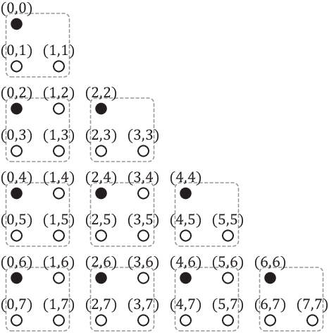
Theorem 3.
The code
| (3) |
is an optimal zero-error code of length and weight for the .
Proof:
The sets of outputs and (hypercubes of sidelength ) are disjoint for every two distinct codewords because, by construction, the coordinate-wise differences are integral multiples of . This proves that the code is zero-error. Observe also that is “perfect”, in the sense that the sets of outputs , , cover the entire space . Indeed, for an arbitrary point , consider the point defined by ; then and . It follows from the result of Shannon [18, Thm 3] that such a perfect code for the is necessarily optimal. (In the terminology of [18], the mapping , , is an “adjacency reducing mapping”.) ∎
Hence, the cardinality of optimal constant-weight codes for this channel is . To determine this quantity explicitly, write in a different form as , where . It follows that
| (4) |
and, by Proposition 2, we have for arbitrary
| (5) |
Theorem 4.
The zero-error capacity of the equals , where is the unique positive real root of the polynomial .
Proof:
The required capacity is equal to the limit of the rates of optimal codes, so we only need to determine the asymptotic behavior of . In order to do this we write in a recurrent form:
| (6) |
with for , which is easily verified from (1) and (5). Since is the solution of the linear recurrence (6), it can be expressed in terms of the roots of its characteristic polynomial [22]. Namely, , where ’s are the roots of and ’s are complex constants determined by the initial conditions11 1 Strictly speaking, the expression is valid only if all the roots are different, so let us verify that they are. Observe that the unique positive root satisfies because . Now, if some had multiplicity two we would have and, by calculating the derivatives of both sides, . This would imply , a contradiction.. It is known [21], [22, Ch. 3, Thm 2] that polynomials of this form (leading coefficient positive, remaining coefficients negative) have a unique positive real root and that the remaining roots cannot exceed in modulus, (in fact, it is easy to show that this inequality is strict in the case of ). This implies that , as claimed. ∎
Finite-Length Performance
It follows from the above proof that (meaning that ), where the constant is determined by the initial conditions of (6). We therefore have a finer asymptotic expansion
| (7) |
which indicates not only the limit of the rates of optimal codes (the capacity), but also the speed of convergence to the limit.
By using Stirling’s approximation, we can also find from (5) the asymptotics of when and , :
| (8) | ||||
where is the binary entropy function. This quantity can be interpreted as the “constant-weight zero-error capacity” of the —the largest rate attainable asymptotically with the requirement that the fraction of the cells containing a particle is (approximately) . Since there are linearly many weights, the zero-error capacity is achievable with constant-weight codes, and so another way to characterize it is
| (9) | ||||
where is the maximizer of . From Stirling’s approximation we can in fact get more information about the asymptotics of the rates of optimal constant-weight codes:
| (10) |
The expressions (7) and (10) are akin to the fundamental bounds on the finite-length performance of optimal codes with non-vanishing error probabilities studied in Shannon theory [19]. Comparing them we see that, even though the capacity can be achieved with constant-weight codes, their finite-length performance is worse than that of general codes. This is quantified by the “second-order” term , which represents the penalty paid for using constant-weight codes.
Some properties of the capacity and related quantities mentioned in this subsection, and their behavior as functions of the channel parameters, are stated in the Appendix.
II-C Additional Noise
In many realistic scenarios the “particles”, apart from being shifted, suffer from other impairments as well. For example, a packet passing through a queuing system may also be received erroneously or may be erased (meaning that the symbol ‘E’ is received instead), see [3, Sec. IV]. Suppose that these additional impairments are modeled by a discrete memoryless channel with input alphabet , with output alphabet not containing22 2 The symbol has a meaning in the shift channel—it represents an empty cell. Therefore, if a symbol could produce a , this would correspond to a deletion of a particle being possible in the compound channel, in which case our analysis would not apply. the symbol , and with zero-error capacity equal to (this channel acts on the particles independently of their shifts; in other words, it acts on the subsequence of the transmitted sequence ). We refer to the compound channel as the Noisy Shift Channel with parameters , or for short.
Theorem 5.
The zero-error capacity of the Noisy Shift Channel equals , where is the unique positive solution to .
Proof:
We only give a brief outline of the proof. A statement analogous to Proposition 2 holds in this case too: if is an optimal zero-error code of length and weight for the , and an optimal zero-error code of length for the discrete memoryless channel acting on the particles, then
| (11) |
is an optimal zero-error code of length and Hamming weight for the . Its cardinality is , and since when , , further analysis is the same as in the proof of Theorem 4 with replaced by (see (5)). ∎
III Zero-error capacity of FIFO queues
We now turn to the analysis of the , a channel introduced as an abstraction of a single-server queue with an infinite buffer. The proofs rely on the methods used in the previous section for the shift channel.
III-A Optimal Codes and the Capacity of the
As for the shift channel, it is enough to solve the constant-weight case with . Also, the set of inputs of length can again be identified with the simplex . Before stating the main result of this section, we describe the construction of optimal codes on a simple example.
Example 2.
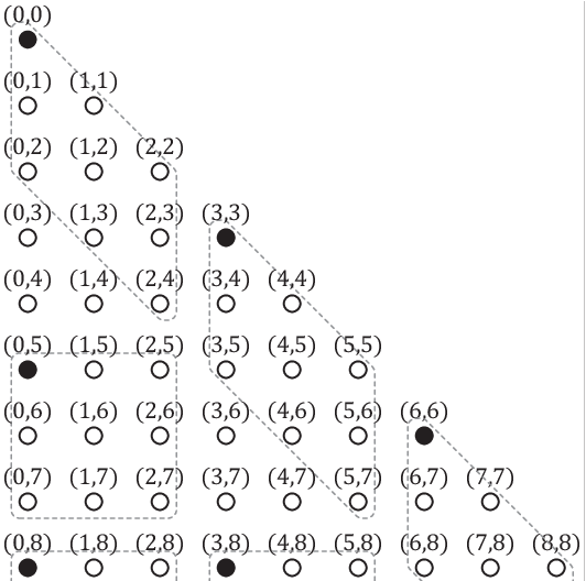
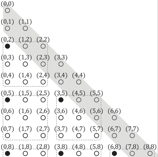
Consider the , and let and . The set of binary sequences of length and weight is represented as the simplex in Figure 2. We construct a code by using a procedure analogous to the one used for the shift channel in [12, Sec. II.B]: List the allowed inputs in the reverse lexicographic order, and in each step select as a codeword the first sequence available on the list that does not conflict with previously chosen codewords, i.e., that cannot produce the same output as one of them. The resulting code is depicted in Figure 2(a). Now observe that we can replace the codewords lying on the right edge of the simplex with other codewords— with , with , and with —without affecting the size of the code and its zero-error property. Note that the points near the right edge represent the sequences whose ’s are too close so that they can “push” each other (think of packets sent in slots not too far apart, so that processing one of them may cause the others to wait in the queue and be further delayed). The result of this replacement of codewords is the same as if we had first forbidden the input sequences with ’s too close to each other, and then constructed a code in the same way as for the shift channel; this is illustrated in Figure 2(b). Namely, the effect of the on the inputs with ’s separated by at least zeros is the same as the effect of the on those inputs—each is shifted for positions to the right. Finally, notice that expelling the sequences with ’s separated by zeros leaves the shape of the space unchanged—it is still a simplex of the same dimension, only smaller.
Theorem 6.
The zero-error capacity of the equals , where .
Proof:
Let denote the size of an optimal zero-error code of length and weight for the (‘Q’ in the superscript stands for ‘Queue’). The code construction described in the previous example can be used in general: 1) Start with , 2) keep only the sequences for which each of the first ’s is followed by at least zeros (at least one such sequence exists if and only if ), 3) in the remaining simplex construct a code in the same way as for the . We shall skip the somewhat tedious argument, but it can be shown that this construction produces an optimal zero-error code when33 3 The greedy construction in the reverse lexicographic order is always optimal, but it does not necessarily give the same number of codewords as the construction given by steps 1)–3). Namely, we have to make sure that the points with which we are replacing the codewords at the edge of the simplex are themselves in the given simplex, see Figure 2; this is why the stated conditions on are needed. and , e.g., via the adjacency reducing mapping theorem [18, Thm 3]. Therefore, for , , we have , where , and so
| (12) |
For general , . The average length of the output sequences is in this case because consecutive packets are separated by at least empty slots by construction and cannot affect each other’s total delay. From this we get, for ,
| (13) | ||||
(For the purpose of determining , it is not a loss of generality to restrict to lengths because one can use zero-padding to satisfy this condition, without affecting the asymptotic rate of codes and their zero-error property.) Now consider the case . For such weights, the construction in the reverse lexicographic order produces at most a polynomial (in ) number of codewords, e.g., for we have . The asymptotic rate will not be reduced if we keep only a single codeword which minimizes the expected output length, and that is ( packets sent in the first slots). This will produce codewords for general , with the expected output length of (see Example 1 in Section I-C). Therefore, for ,
| (14) |
Finally, maximizing over all (see (13) and (14)) gives the expression for the zero-error capacity. ∎
The capacity-achieving strategy is very simple: If the capacity equals it can be achieved by inserting zeros/empty slots after every symbol of the information sequence written in the alphabet , and if it equals the capacity-achieving code is .
III-B Additional Noise
Suppose that the packets, apart from being delayed in the queue, experience other types of impairments as well. Suppose further that these additional impairments are modeled as a discrete memoryless channel with input alphabet , with output alphabet not containing the symbol , and with the zero-error capacity equal to (this channel acts on the packets independently of their passing through the queue, i.e., it acts on the subsequence of the transmitted sequence ). We refer to the compound channel as the Noisy with parameters , or for short.
Theorem 7.
The zero-error capacity of the equals .
IV Zero-error detection
In some situations, it is required of the receiver only to detect that a specific kind of error has happened, not necessarily to correct it. A code is said to be zero-error-detecting for a given channel if it ensures that all possible errors allowed in the model can be detected, meaning that the receiver can conclude with probability one whether the transmission was error-free or not. We shall assume that every input sequence can produce itself at the channel output, i.e., , because otherwise the detection is trivial (for the this amounts to assuming ). If this is the case, then an equivalent way of stating the zero-error-detection property of a code is that no codeword can produce another codeword at the channel output. This condition is less stringent compared to the definition of zero-error code (which will be called zero-error-correcting in this section, to avoid confusion): two codewords are now allowed to produce the same output , but as long as itself is not a codeword, the receiver will recognize that an error has occurred. The zero-error-detection capacity [7, 2] of a channel is the of the rates of optimal zero-error-detecting codes of length for that channel.
IV-A The Shift Channel
Unlike in the error-correction case, the channels and are not equivalent from the point of view of error-detection, i.e., the analog of Lemma 1 does not hold here. As an example, consider the code which is zero-error-detecting in the , but is not zero-error-detecting in the , because in the latter case . However, the analog of Proposition 2 holds and enables one to focus on the case .
The following claim describes a relation between zero-error-detecting and zero-error-correcting codes for the shift channel.
Proposition 8.
Let .
- (a)
Every zero-error-detecting code for the is a zero-error-correcting code for the .
- (b)
Every zero-error-correcting code for the is a zero-error-detecting code for the .
In particular, a code is zero-error-detecting for the if and only if it is zero-error-correcting for the .
Proof:
Assume w.l.o.g. that , and recall the geometric representation of the code space as described in Section II-B (constant-weight case, ). Let be a codeword. That a code is zero-error-detecting for the means that every hypercube of the form is such that it does not contain a codeword other than . This, together with the assumption , implies that the hypercubes , formed in this way for every codeword , are pairwise disjoint, meaning that the code is zero-error-correcting for the . The statement (b) is deduced in a similar way from the geometric interpretation of the involved notions. ∎
Consequently, the zero-error-detection capacity of the is lower bounded by the zero-error-correction capacity of the and upper bounded by the zero-error-correction capacity of the . We next prove that this upper bound can always be achieved.
Theorem 9.
Let . The zero-error-detection capacity of the is equal to , where is the unique positive real root of the polynomial .
Proof:
Again, assume that . As remarked above, Proposition 8() implies that the zero-error-detection capacity of the is upper bounded by the zero-error-correction capacity of the , which is precisely by Theorem 4. To prove the claim we need to demonstrate that the rate is achievable, and this is done by exhibiting a family of codes with the desired properties. Define
| (15) | ||||
where (recall that ). Note that is a subcode of the code from (3), obtained as its intersection with the hyperplane . We have
| (16) |
and so, for every and , there is at least one for which it holds that
| (17) |
Therefore, for ’s chosen in this way, the codes
have asymptotically the same rate as the codes , which
is for .
It is left to verify that the codes
are indeed zero-error-detecting for the .
Suppose that a codeword was
transmitted and a sequence received at the output of the channel.
If , the receiver will easily recognize an error, so suppose
that .
In this case, if any shifts have occurred in the channel, some of them must have
been shifts to the right and some of them shifts to the left for otherwise we could
not have .
Suppose that the ’th particle was shifted to the right, .
Then, since and ,
we have , so cannot
be a codeword.
Therefore, the receiver can detect all errors allowed in the model.
∎
Notice that the zero-error-detection capacity of the equals for every , as if there were no shifts at all.
IV-B FIFO Queues
In the model only shifts to the right are possible, which makes the detection problem very easy (see also the last remark in the previous subsection).
Theorem 10.
The zero-error-detection capacity of the is equal to .
Proof:
The value is clearly an upper bound on the capacity because is the cardinality of the input alphabet, so it is left to prove achievability. The codes
| (18) |
are zero-error-detecting for the . Their cardinality, for appropriately chosen , satisfies
| (19) |
Multiplying the above expression by , taking the logarithm, normalizing by
, and letting , , we get a lower bound on the
asymptotic rate of optimal constant-weight zero-error-detecting codes for the
in the form .
The maximum of this function over is precisely .
An important point to emphasize here is that the rate was computed by normalizing by
, and not by as in the error-correction case.
The reason is the following: since we are using constant-weight codes, and since
we are only trying to detect the shifts, the receiver can stop looking at the output
after the ’th slot because if some of the packets have been delayed for more
that, it can detect this by counting the received packets in the first
slots.
The actual rate of the code in the error-detection
context is therefore .
∎
V Continuous-time models
In this section we introduce and analyze the continuous-time versions of the shift and queuing channels studied up to this point. The reasoning is analogous to the discrete-time case so we give only a brief outline.
Throughout the section we shall assume that the probability distribution of particle/packet delays is absolutely continuous with respect to the Lebesgue measure. This assumption, in particular, ensures the existence of an optimal decoding rule, i.e., decoding rule that minimizes the error probability. A code will be called zero-error if its error probability (under an optimal decoding rule) is equal to zero.
Remark 4 (Zero-error codes).
Recall (Section I-C) that, in the discrete-time case, a code is said to be zero-error if either of the following two equivalent conditions holds:
(c1) the error probability under optimal decoding is equal to zero, and (c2) no two codewords can produce the same output.These two requirements are in general not equivalent in the continuous-time case—the error probability for a given code can be zero even if two different codewords can produce the same output, because there are uncountably many possible outputs. However, it should be noted that both of these definitions result in the same value of the zero-error capacity. The reason we have adopted (c1) as the definition of zero-error codes in this section is that this convention slightly simplifies the proofs.
V-A Continuous-Time Shift Channels
We describe the continuous-time version of the shift channel in the context of queuing systems. Suppose that the transmitter can send packets from a -ary alphabet at arbitrary instants of time, but with the restriction that any two emissions are separated by at least seconds (think of as the time needed to physically transmit a single packet). Suppose that packets were transmitted in a given interval (the code “length” is now a continuous parameter ). Every such input of duration and weight is uniquely specified (for ) by the sequence of emission times , . Therefore, the set of all inputs of duration and weight is in a one-to-one correspondence with the simplex (for convenience, we have scaled the emission times with and subtracted the vector from them; this is how the latter representation was obtained).
We further assume that the ’th packet is delayed in the channel for a random amount of time , but that reordering of packets is not possible. The probability distribution of is assumed to be absolutely continuous with respect to the Lebesgue measure, with the corresponding density strictly positive on . In other words, the packets are processed in a FIFO manner and the total time that any packet spends in the system—the so-called residence time—is bounded by . Using the above notation, the set of outputs can be represented as the hypercube of sidelength with at its corner (restricted to the simplex), namely . We refer to the channel just described as the -ary Continuous-Time Shift Channel, .
Theorem 11.
The zero-error capacity of the equals , where is the unique positive solution to .
Proof:
As in the discrete case, codewords can be chosen so that the hypercubes pack the simplex perfectly, implying that the resulting code is optimal, see Theorem 3. (In the continuous case we allow the decoding regions to overlap, but their intersection is required to have measure zero, see Remark 4; in other words, the hypercubes can touch along their faces only.) If , the cardinality of the resulting code will be, similarly to (5), . The constant-weight zero-error capacity is the limit of the rate of these codes as and . The zero-error capacity is then obtained by maximizing over and can be characterized as , where is the unique positive solution of . If , the capacity is trivially . ∎
V-B Continuous-Time FIFO Queues
Consider now the continuous-time analog of the . As for the , we assume that the transmitter is sending packets from a -ary alphabet at arbitrary instants of time, with the restriction that any two emissions are separated by at least seconds. Further, we assume that the processing time of each packet is a random variable with distribution absolutely continuous with respect to the Lebesgue measure, and with the corresponding density strictly positive on the interval . The service procedure is FIFO. We refer to this model as the -ary Continuous-Time Queue with bounded Processing Time, or for short.
Theorem 12.
The zero-error capacity of the is , where . ∎
Notice that the capacity of the is independent of when this parameter is small. This is an important difference compared to the continuous-time shift channel discussed in the previous subsection. For example, when the emission time , the zero-error capacity of the grows to infinity. This is expected because means that we can send an unbounded number of packets in any given interval of time, while the delay of each of them is bounded by a constant . In the , however, sending more packets also means that the time needed to receive them will be much longer on average, and the rate in fact remains unchanged.
VI Concluding remarks
Channels with symbol shifts as the dominant type of noise are well-motivated communication models. In the present paper two classes of such channels were studied, both in discrete and continuous time, and a characterization of their zero-error capacity and zero-error-detection capacity was obtained. To conclude the paper, we mention two possible extensions of these models as directions for further work; we believe that these extensions are natural and important in the context of the mentioned applications.
One of the extensions refers to models that include deletions of particles/packets. One can imagine a queuing system with a finite buffer which drops an incoming packet whenever the buffer is full, or a molecular communication system in which some of the particles never arrive at the receiving side. Another extension are models in which reordering of particles/packets is allowed (see, e.g., [1, 9, 14]). For example, due to properties of most molecular communication systems, it is reasonable to assume that the order in which the particles arrive at the receiving side is not necessarily the same as the one in which they were transmitted. If the particles are identical, then this reordering has no effect on information transfer and the analysis is the same as for the [12]; however, the case seems to be much more difficult and the corresponding analysis would require different methods than the ones used here.
Precisely defining and analyzing models similar to those studied in this paper, but which also include deletions and/or out-of-order arrival of packets, is an interesting problem for future investigation.
Acknowledgment
The authors would like to thank the three anonymous reviewers for their comments which greatly improved the presentation of this work.
References
- [1] R. Ahlswede and A. H. Kaspi, “Optimal Coding Strategies for Certain Permuting Channels,” IEEE Trans. Inf. Theory, vol. 33, no. 3, pp. 310–314, May 1987.
- [2] R. Ahlswede, N. Cai, and Z. Zhang, “Erasure, List, and Detection Zero-Error Capacities for Low Noise and a Relation to Identification,” IEEE Trans. Inf. Theory, vol. 42, no. 1, pp. 55–62, Jan. 1996.
- [3] V. Anantharam and S. Verdú, “Bits Through Queues,” IEEE Trans. Inf. Theory, vol. 42, no. 1, pp. 4–18, Jan. 1996.
- [4] A. S. Bedekar and M. Azizog̃lu, “The Information-Theoretic Capacity of Discrete-Time Queues,” IEEE Trans. Inf. Theory, vol. 44, no. 2, pp. 446–461, Mar. 1998.
- [5] S. Engelberg and O. Keren, “Reliable Communications Across Parallel Asynchronous Channels With Arbitrary Skews,” IEEE Trans. Inf. Theory, vol. 63, no. 2, pp. 1120–1129, Feb. 2017.
- [6] N. Farsad, H. B. Yilmaz, A. Eckford, C.-B. Chae, and W. Guo, “A Comprehensive Survey of Recent Advancements in Molecular Communication,” IEEE Commun. Surveys Tuts., vol. 18, no. 3, pp. 1887–1919, 2016.
- [7] L. Gargano, J. Körner, and U. Vaccaro, “Qualitative Independence and Sperner Problems for Directed Graphs,” J. Combin. Theory Ser. A, vol. 61, no. 2, pp. 173–192, Nov. 1992.
- [8] K. A. S. Immink, “Runlength-Limited Sequences,” Proc. IEEE, vol. 78, no. 11, pp. 1745–1759, Nov. 1990.
- [9] K. Kobayashi, “Combinatorial Structure and Capacity of the Permuting Relay Channel,” IEEE Trans. Inf. Theory, vol. 33, no. 6, pp. 813–826, Nov. 1987.
- [10] J. Körner and A. Orlitsky, “Zero-Error Information Theory,” IEEE Trans. Inf. Theory, vol. 44, no. 6, pp. 2207–2229, Oct. 1998.
- [11] M. Kovačević, “A Note on Parallel Asynchronous Channels With Arbitrary Skews,” IEEE Trans. Inf. Theory, to appear.
- [12] M. Kovačević and P. Popovski, “Zero-Error Capacity of a Class of Timing Channels,” IEEE Trans. Inf. Theory, vol. 60, no. 11, pp. 6796–6800, Nov. 2014.
- [13] V. Yu. Krachkovsky, “Bounds on the Zero-Error Capacity of the Input-Constrained Bit-Shift Channel,” IEEE Trans. Inf. Theory, vol. 40, no. 4, pp. 1240–1244, Jul. 1994.
- [14] M. Langberg, M. Schwartz, and E. Yaakobi, “Coding for the -Limited Permutation Channel,” in Proc. 2015 IEEE Int. Symp. Inf. Theory (ISIT), pp. 1936–1940, Hong Kong, Jun. 2015.
- [15] T. Nakano, A. W. Eckford, and T. Haraguchi, Molecular Communication, Cambridge University Press, 2013.
- [16] S. H. Sellke, C.-C. Wang, N. Shroff, and S. Bagchi, “Capacity Bounds on Timing Channels with Bounded Service Times,” in Proc. 2007 IEEE Int. Symp. Inf. Theory (ISIT), pp. 981–985, Nice, France, Jun. 2007.
- [17] S. Shamai (Shitz) and E. Zehavi, “Bounds on the Capacity of the Bit-Shift Magnetic Recording Channel,” IEEE Trans. Inf. Theory, vol. 37, no. 3, pp. 863–872, May 1991.
- [18] C. E. Shannon, “The Zero Error Capacity of a Noisy Channel,” IRE Trans. Inf. Theory, vol. 2, no. 3, pp. 8–19, Sep. 1956.
- [19] V. Y. F. Tan, “Asymptotic Estimates in Information Theory with Non-Vanishing Error Probabilities,” Foundations and Trends in Communications and Information Theory, vol. 11, nos. 1-2, pp. 1–184, 2014.
- [20] J. A. Thomas, “On the Shannon Capacity of Discrete Time Queues,” in Proc. 1997 IEEE Int. Symp. Inf. Theory (ISIT), p. 333, Ulm, Germany, Jun./Jul. 1997.
- [21] H. S. Wilf, “Perron-Frobenius Theory and the Zeros of Polynomials,” Proc. Amer. Math. Soc., vol. 12, no. 2, pp. 247–250, Apr. 1961.
- [22] H. S. Wilf, Mathematics for the Physical Sciences, Dover Publications, Inc., 1978.
We list here several properties of the zero-error capacity of the and related quantities, regarded as functions of the channel parameters. The parameters and are assumed to be integers taking values and . Whenever the behavior of a function with respect to one variable is discussed, it is understood that the remaining variables/parameters are kept fixed.
Proposition 13.
The function , defined by , , is
- (a)
Continuous, monotonically decreasing, and convex in , with and ;
- (b)
Continuous, monotonically increasing, and convex in , with .
The function is
- (c)
Continuous, monotonically decreasing, and convex in ;
- (d)
Continuous, monotonically increasing in , and concave over .
Proof:
The functions and are well-defined for arbitrary real (not necessarily integer) and in the specified ranges. The claim is obtained by differentiating them, e.g.,
| (20) |
and verifying the sign of the derivatives. ∎
The function is even easier to analyze since it is explicit, see (8).
Proposition 14.
The function is
- (a)
Continuous, monotonically decreasing, and convex in ;
- (b)
Continuous, monotonically increasing, and concave in ;
- (c)
Continuous and concave in . ∎
The values/limits of at , , , , and , can be found directly from (8).
Finally, we state several properties of the weight (the fraction of occupied cells) which optimizes the rate of a constant-weight code.
Proposition 15.
Define . The function has the following properties:
- (a)
;
- (b)
It is continuous, monotonically increasing in , and concave over ;
- (c)
For , it is monotonically increasing in , with ;
For , it is monotonically decreasing in , with . ∎
Proof:
Equating the derivative of with zero we get that is the solution of
| (21) |
Letting , (21) becomes , which means that . This proves (a). (b) is shown by calculating the derivatives of from (a). To prove (c), it is enough to demonstrate that the function is monotonically decreasing to for , and monotonically increasing to for , which can again be shown by analyzing its derivative. ∎