跳到论文正文
W Papers独立论文阅读器 arXiv:1605.02121 论文正文 计算阅读时间 · 0%
引用这篇论文根据当前论文元数据生成,正式投稿前建议核对。


License: arXiv.org perpetual non-exclusive license
arXiv:1605.02121v5 [math.NA] 13 Sep 2018

Convergence Rate for a Radau hp Collocation Method Applied to Constrained Optimal Control Thanks:  October 24, 2017, revised September 11, 2018. The authors gratefully acknowledge support by the Office of Naval Research under grants N00014-11-1-0068, N00014-15-1-2048, and N00014-18-1-2100, by the National Science Foundation under grants DMS-1522629, CBET-1404767, and DMS-1819002, and by the U.S. Air Force Research Laboratory under contract FA8651-08-D-0108/0054.

William W. Hager ††thanks: hager@ufl.edu, http://people.clas.ufl.edu/hager/, PO Box 118105, Department of Mathematics, University of Florida, Gainesville, FL 32611-8105. Phone (352) 294-2308. Fax (352) 392-8357.    Hongyan Hou ††thanks: hongyan.hou@mnstate.edu, Mathematics Department, Minnesota State University Moorhead, P.O. Box 104, 1104 7th Avenue South, Moorhead, MN 56563 Phone (218) 477-4007.    Subhashree Mohapatra ††thanks: subha@ufl.edu, Department of Mathematics, University of Florida, Gainesville, FL 32611.    Anil V. Rao ††thanks: anilvrao@ufl.edu, http://www.mae.ufl.edu/rao, Department of Mechanical and Aerospace Engineering, P.O. Box 116250, Gainesville, FL 32611-6250. Phone (352) 392-0961. Fax:(352) 392-7303.    Xiang-Sheng Wang ††thanks: xswang@louisiana.edu, http://www.ucs.louisiana.edu/$∼$xxw6637/, Department of Mathematics, University of Louisiana at Lafayette, Lafayette, LA 70503. Phone (337) 482-5281.
Abstract

For control problems with control constraints, a local convergence rate is established for an h​php-method based on collocation at the Radau quadrature points in each mesh interval of the discretization. If the continuous problem has a sufficiently smooth solution and the Hamiltonian satisfies a strong convexity condition, then the discrete problem possesses a local minimizer in a neighborhood of the continuous solution, and as either the number of collocation points or the number of mesh intervals increase, the discrete solution convergences to the continuous solution in the sup-norm. The convergence is exponentially fast with respect to the degree of the polynomials on each mesh interval, while the error is bounded by a polynomial in the mesh spacing. An advantage of the h​php-scheme over global polynomials is that there is a convergence guarantee when the mesh is sufficiently small, while the convergence result for global polynomials requires that a norm of the linearized dynamics is sufficiently small. Numerical examples explore the convergence theory.

keywords
hp collocation, Radau collocation, convergence rate, optimal control, orthogonal collocation
AMS
49M25, 49M37, 65K05, 90C30

1 Introduction

A convergence rate is established for an h​php-orthogonal collocation method applied to a constrained control problem of the form

minimizeC⁡(𝐱⁡(1))subject to𝐱˙​(t)=𝐟⁡(𝐱⁡(t),𝐮⁡(t)),𝐮(t)∈𝒰,t∈Ω0,𝐱⁡(0)=𝐚,(𝐱,𝐮)∈𝒞1​(Ω0)×𝒞0​(Ω0),}\left.\begin{array}[]{cll}\mbox{minimize}&C({\bf{x}}(1))&\\ \mbox{subject to}&\dot{{\bf{x}}}(t)={\bf{f(x}}(t),{\bf{u}}(t)),&{\bf{u}}(t)\in{\cal{U}},\quad t\in\Omega_{0},\\ &{\bf{x}}(0)={\bf{a}},&({\bf{x}},{\bf{u}})\in{\cal{C}}^{1}(\Omega_{0})\times{\cal{C}}^{0}(\Omega_{0}),\end{array}\right\} (1)

where Ω0=[0,1]\Omega_{0}=[0,1], the control constraint set 𝒰⊂ℝm{\cal{U}}\subset\mathbb{R}^{m} is closed and convex with nonempty interior, the state 𝐱⁡(t)∈ℝn{{\bf{x}}}(t)\in\mathbb{R}^{n}, 𝐱˙\dot{{\bf{x}}} denotes the derivative of 𝐱{\bf{x}} with respect to tt, 𝐟:ℝn×ℝm→ℝn{{\bf{f}}}:{\mathbb{R}}^{n}\times{\mathbb{R}}^{m}\rightarrow{\mathbb{R}}^{n}, C:ℝn→ℝC:{\mathbb{R}}^{n}\rightarrow{\mathbb{R}}, and 𝐚{{\bf{a}}} is the initial condition, which we assume is given; 𝒞l​(Ω0){\cal{C}}^{l}(\Omega_{0}) denotes the space of ll times continuously differentiable functions mapping Ω0\Omega_{0} to ℝd\mathbb{R}^{d} for some dd. The value of dd should be clear from context; states and costates always have nn components and controls have mm components. It is assumed that 𝐟{\bf{f}} and CC are at least continuous. When the dynamics in (1) can be solved for the state 𝐱{\bf{x}} as a function of the control 𝐮{\bf{u}}, the control problem reduces to a constrained minimization over 𝐮{\bf{u}}.

The development of h​php-techniques in the context of finite element methods for boundary-value problems began with the work of Babuška and Gui in [25, 26, 27], and Babuška and Suri in [1, 2, 3]. In the h​php-collocation approach that we develop for (1), the time domain Ω0\Omega_{0} is initially partitioned into a mesh. To simplify the discussion, we focus on a uniform mesh consisting of KK intervals [tk−1,tk][t_{k-1},t_{k}] defined by the mesh points tk=k/Kt_{k}=k/K where 0≤k≤K0\leq k\leq K. The dynamics of (1) are reformulated using a change of variables. Let tk+1/2=(tk+tk+1)/2t_{k+1/2}=(t_{k}+t_{k+1})/2 be the midpoint of the mesh interval [tk,tk+1][t_{k},t_{k+1}]. We make the change of variables t=tk−1/2+h​τt=t_{k-1/2}+h\tau, where h=1/(2​K)h=1/(2K) is half the width of the mesh interval and τ∈Ω:=[−1,1]\tau\in\Omega:=[-1,1]; let us define 𝐱k:Ω→ℝn{\bf{x}}_{k}:\Omega\rightarrow\mathbb{R}^{n} by 𝐱k​(τ)=𝐱⁡(tk−1/2+h​τ){\bf{x}}_{k}(\tau)={\bf{x}}(t_{k-1/2}+h\tau). Thus 𝐱k{\bf{x}}_{k} corresponds to the restriction of 𝐱{\bf{x}} to the mesh interval [tk−1,tk][t_{k-1},t_{k}]. Similarly, we define a control 𝐮k{\bf{u}}_{k} corresponding to the restriction of 𝐮{\bf{u}} to the mesh interval [tk−1,tk][t_{k-1},t_{k}]. In the new variables, the control problem reduces to finding KK state-control pairs (𝐱k,𝐮k)({\bf{x}}_{k},{\bf{u}}_{k}), 1≤k≤K1\leq k\leq K, each pair defined on the interval [−1,1][-1,1], to solve the problem

minimizeC​(𝐱K​(1))subject to𝐱˙k(τ)=h𝐟(𝐱k(τ),𝐮k(τ)),𝐮k(τ)∈𝒰,τ∈Ω,𝐱k​(−1)=𝐱k−1​(1),1≤k≤K,(𝐱k,𝐮k)∈𝒞1​(Ω)×𝒞0​(Ω).}\left.\begin{array}[]{cll}\mbox{minimize}&C({\bf{x}}_{K}(1))&\\ \mbox{subject to}&\dot{{\bf{x}}}_{k}(\tau)=h{\bf{f(x}}_{k}(\tau),{\bf{u}}_{k}(\tau)),\quad{\bf{u}}_{k}(\tau)\in{\cal{U}},&\tau\in\Omega,\\ &{\bf{x}}_{k}(-1)={\bf{x}}_{k-1}(1),&1\leq k\leq K,\\ &({\bf{x}}_{k},{\bf{u}}_{k})\in{\cal{C}}^{1}(\Omega)\times{\cal{C}}^{0}(\Omega).\end{array}\right\} (2)

Since the function 𝐱0{\bf{x}}_{0} does not exist (there is no 0-th mesh interval), we simply define 𝐱0​(1)=𝐚{\bf{x}}_{0}(1)={\bf{a}}, the initial condition. The condition

𝐱k​(−1)=𝐱k−1​(1){\bf{x}}_{k}(-1)={\bf{x}}_{k-1}(1) (3)

in (2) corresponds to the initial condition 𝐱⁡(0)=𝐚{\bf{x}}(0)={\bf{a}} when k=1k=1 and to continuity of the state across a mesh interval boundary when k>1k>1. Throughout the paper, (3) is referred to as the continuity condition.

In the h​php-scheme developed in this paper, the dynamics for 𝐱k{\bf{x}}_{k} are approximated by the Radau collocation scheme developed in [10, 22, 23, 31]. Let 𝒫N{\cal{P}}_{N} denote the space of polynomials of degree at most NN defined on the interval Ω\Omega, and let 𝒫Nn{\cal{P}}_{N}^{n} denote the nn-fold Cartesian product 𝒫N×…×𝒫N{\cal{P}}_{N}\times\ldots\times{\cal{P}}_{N}. We analyze a discrete approximation to (2) of the form

minimizeC​(𝐱K​(1))subject to𝐱˙k​(τi)=h​𝐟​(𝐱k​(τi),𝐮k​i),1≤i≤N,𝐮k​i∈𝒰,𝐱k​(−1)=𝐱k−1​(1),1≤k≤K,𝐱k∈𝒫Nn.}\left.\begin{array}[]{cll}\mbox{minimize}&C({\bf{x}}_{K}(1))&\\ \mbox{subject to}&\dot{{\bf{x}}}_{k}(\tau_{i})=h{\bf{f}}({\bf{x}}_{k}(\tau_{i}),{\bf{u}}_{ki}),&1\leq i\leq N,\;{\bf{u}}_{ki}\in{\cal{U}},\\ &{\bf{x}}_{k}(-1)={\bf{x}}_{k-1}(1),&1\leq k\leq K,\;{\bf{x}}_{k}\in{\cal{P}}_{N}^{n}.\end{array}\right\} (4)

Note that there is no polynomial associated with the control; 𝐮k​i{\bf{u}}_{ki} corresponds to the value of the control at tk−1/2+h​τit_{k-1/2}+h\tau_{i}. In (4) the dimension of 𝒫N{\cal{P}}_{N} is N+1N+1 and there are KK mesh intervals, so a component of the state variable is chosen from a space of dimension K⁡(N+1)K(N+1). Similarly, there are K​N+KKN+K equations in (4) corresponding to the collocated dynamics at K​NKN points and the KK continuity conditions, the initial condition at t=0t=0 and the K−1K-1 continuity conditions for the state at the interior mesh points.

For simplicity in the analysis, the same degree polynomials are used in each mesh interval, while in practical implementations of the h​php-scheme [10, 11, 38, 40], polynomials of different degrees are often used on different intervals. On intervals where the solution is smooth, high degree polynomials are employed, while on intervals where the solution is nonsmooth, low degree polynomials are used.

We focus on a collocation scheme based on the NN Radau quadrature points satisfying

−1<τ1<τ2<…<τN=1.-1<\tau_{1}<\tau_{2}<\ldots<\tau_{N}=1.

The Radau points are related to the zeros of a Jacobi polynomial. Recall that the Jacobi polynomials PN(α,β)P^{(\alpha,\beta)}_{N} are a class of polynomials orthogonal with respect to the weight (1−τ)α​(1+τ)β(1-\tau)^{\alpha}(1+\tau)^{\beta} for τ∈[−1,1]\tau\in[-1,1]; the subscript NN specifies the polynomial degree. The interior Radau abscissa τi\tau_{i}, 1≤i≤N−11\leq i\leq N-1, are the zeros of the Jacobi polynomial PN−1(1,0)P^{(1,0)}_{N-1} associated with the weight 1−τ1-\tau. These quadrature points are sometimes called the flipped Radau points, while the standard Radau points are −τi-\tau_{i}, 1≤i≤N1\leq i\leq N. The analysis is the same for either set of points, while the notation is a little cleaner for the flipped points. Besides the NN collocation points, our analysis also utilizes the noncollocated point τ0=−1\tau_{0}=-1.

It is pointed out in [32] that for a global collocation scheme where K=1K=1, the discrete dynamics may be infeasible for certain choices of NN. In contrast, the analysis in this paper implies that locally, for each choice of the discrete control, there exists a unique discrete state which satisfies the discrete dynamics when KK is sufficiently large, or equivalently, when hh is sufficiently small, regardless of the choice for NN. In this respect, the h​php-collocation approach is more robust than a global scheme.

Other global collocation schemes that have been presented in the literature are based on the Lobatto quadrature points [17, 20], on the Chebyshev quadrature points [18, 21], on the Gauss quadrature points [4, 23], and on the extrema of Jacobi polynomials [45]. Kang [36, 37] considers control systems in feedback linearizable normal form, and shows that when the Lobatto discretized control problem is augmented with bounds on the states and control, and on certain Legendre polynomial expansion coefficients, then the objectives in the discrete problem converge to the optimal objective of the continuous problem at an exponential rate. Kang’s analysis does not involve coercivity assumptions for the continuous problem, but instead imposes bounds in the discrete problem. Also, in [24] a consistency result is established for a scheme based on Lobatto collocation.

Any of the global schemes could be developed into an h​php-collocation scheme. Our rationale for basing our h​php-scheme on the Radau collocation points was the following: In numerical experiments such as those in [23], there is often not much difference between the convergence speed of approximations based on either Gauss or Radau collocation, while the Lobatto scheme often converged much slower; and in some cases, the Lobatto costate approximation did not converge due to a null space that arises in the first-order optimality conditions – see [23]. On the other hand, the implementation of an h​php-scheme based on the Radau quadrature points was much simpler than the implementation based on the Gauss quadrature points. The Gauss points lie in the interior of each mesh interval, which requires the introduction of the state value at the mesh points. Since one of the Radau points is a mesh point, there is no need to introduce an additional noncollocated point. The implementation ease of Chebyshev quadrature should be similar to that of Gauss and was not pursued. The h​php-collocation scheme analyzed in this paper corresponds to the scheme implemented in the popular GPOPS-II software package [42] for solving optimal control problems. This paper, in essence, provides a theoretical justification for the algorithm implemented in the software.

For 𝐱∈𝒞0​(Ω0){\bf{x}}\in{\cal{C}}^{0}(\Omega_{0}), we use the sup-norm ∥⋅∥∞\|\cdot\|_{\infty} given by

‖𝐱‖∞=sup{|𝐱⁡(t)|:t∈Ω0},\|{\bf{x}}\|_{\infty}=\sup\{|{\bf{x}}(t)|:t\in\Omega_{0}\},

where |⋅||\cdot| is the Euclidean norm. Given 𝐲∈ℝn{\bf{y}}\in\mathbb{R}^{n}, the ball with center 𝐲{\bf{y}} and radius ρ\rho is denoted

ℬρ​(𝐲)={𝐱∈ℝn:|𝐱−𝐲|≤ρ}.{\cal{B}}_{\rho}({\bf{y}})=\{{\bf{x}}\in\mathbb{R}^{n}:|{\bf{x}}-{\bf{y}}|\leq\rho\}.

The following regularity assumption is assumed to hold throughout the paper.

Smoothness. The problem (1) has a local minimizer (𝐱∗,𝐮∗)({\bf{x}}^{*},{\bf{u}}^{*}) in 𝒞1​(Ω0)×𝒞0​(Ω0){\cal{C}}^{1}(\Omega_{0})\times{\cal{C}}^{0}(\Omega_{0}). For some ρ>0\rho>0 and open set 𝒪⊂ℝm+n{\cal{O}}\subset\mathbb{R}^{m+n} such that

ℬρ​(𝐱∗​(t),𝐮∗​(t))⊂𝒪​ for all ​t∈Ω0,{\cal{B}}_{\rho}({\bf{x}}^{*}(t),{\bf{u}}^{*}(t))\subset{\cal{O}}\mbox{ for all }t\in\Omega_{0},

the first two derivative of ff and CC are Lipschitz continuous on the closure of 𝒪{\cal{O}} and on ℬρ​(𝐱∗​(1)){\cal{B}}_{\rho}({\bf{x}}^{*}(1)) respectively.

Let 𝝀∗\bm{\lambda}^{*} denote the solution of the linear costate equation

𝝀˙∗​(t)=−∇xH​(𝐱∗​(t),𝐮∗​(t),𝝀∗​(t)),𝝀∗​(1)=∇C​(𝐱∗​(1)),\dot{\bm{\lambda}}^{*}(t)=-\nabla_{x}H({{\bf{x}}}^{*}(t),{{\bf{u}}}^{*}(t),{\bm{\lambda}}^{*}(t)),\quad{\bm{\lambda}}^{*}(1)=\nabla C({{\bf{x}}}^{*}(1)), (5)

where HH is the Hamiltonian defined by H⁡(𝐱,𝐮,𝝀)=𝝀𝖳​𝐟​(𝐱,𝐮)H({{\bf{x}}},{{\bf{u}}},{\bm{\lambda}})={\bm{\lambda}}^{\sf T}{{\bf{f}}}({{\bf{x}}},{{\bf{u}}}) and ∇\nabla denotes gradient. By the first-order optimality conditions (Pontryagin’s minimum principle), we have

−∇uH​(𝐱∗​(t),𝐮∗​(t),𝝀∗​(t))∈N𝒰​(𝐮∗​(t))​ for all ​t∈Ω0.-\nabla_{u}H({{\bf{x}}}^{*}(t),{{\bf{u}}}^{*}(t),{\bm{\lambda}}^{*}(t))\in N_{{\cal{U}}}({\bf{u}}^{*}(t))\mbox{ for all }t\in\Omega_{0}. (6)

For any 𝐮∈𝒰{\bf{u}}\in{\cal{U}},

N𝒰​(𝐮)={𝐰∈ℝm:𝐰𝖳​(𝐯−𝐮)≤0​ for all ​𝐯∈𝒰},N_{\cal{U}}({\bf{u}})=\{{\bf{w}}\in\mathbb{R}^{m}:{\bf{w}}^{\sf T}({\bf{v}}-{\bf{u}})\leq 0\mbox{ for all }{\bf{v}}\in{\cal{U}}\},

while N𝒰​(𝐮)=∅N_{\cal{U}}({\bf{u}})=\emptyset if 𝐮∉𝒰{\bf{u}}\not\in{\cal{U}}.

We will show in Proposition 2 that the first-order optimality conditions (Karush-Kuhn-Tucker conditions) for (4) are equivalent to the existence of 𝝀k∈𝒫N−1n\bm{\lambda}_{k}\in{\cal{P}}_{N-1}^{n}, 1≤k≤K1\leq k\leq K, such that

𝝀˙k​(τi)\displaystyle\dot{\bm{\lambda}}_{k}(\tau_{i}) =\displaystyle= −h​∇xH​(𝐱k​(τi),𝐮k​i,𝝀k​(τi)),1≤i<N,\displaystyle-h\nabla_{x}H\left({{\bf{x}}}_{k}(\tau_{i}),{{\bf{u}}}_{ki},{\bm{\lambda}}_{k}(\tau_{i})\right),\quad 1\leq i<N, (7)
𝝀˙k​(1)\displaystyle\dot{\bm{\lambda}}_{k}(1) =\displaystyle= −h​∇xH​(𝐱k​(1),𝐮k​N,𝝀k​(1))+(𝝀k​(1)−𝝀k+1​(−1))/ωN,\displaystyle-h\nabla_{x}H\left({{\bf{x}}}_{k}(1),{{\bf{u}}}_{kN},{\bm{\lambda}}_{k}(1)\right)+\left(\bm{\lambda}_{k}(1)-{\bm{\lambda}}_{k+1}(-1)\right)/\omega_{N}, (8)
where ​𝝀K+1​(−1):=∇C​(𝐱K​(1))\displaystyle\quad\quad\mbox{where }\bm{\lambda}_{K+1}(-1):=\nabla C\left({\bf{x}}_{K}(1)\right)
N𝒰​(𝐮k​i)\displaystyle N_{\cal{U}}({\bf{u}}_{ki}) ∋\displaystyle\ni −∇uH​(𝐱k​(τi),𝐮k​i,𝝀k​(τi)),1≤i≤N.\displaystyle-\nabla_{u}H\left({{\bf{x}}}_{k}(\tau_{i}),{{\bf{u}}}_{ki},{\bm{\lambda}}_{k}(\tau_{i})\right),\quad 1\leq i\leq N. (9)

Since the K+1K+1 mesh interval does not exist, (8) includes a definition for 𝝀K+1​(−1)\bm{\lambda}_{K+1}(-1). As we will see in Proposition 2, 𝝀k​(−1)\bm{\lambda}_{k}(-1) for k≤Kk\leq K is the multiplier associated with the continuity condition (3). Throughout the paper, ωi\omega_{i}, 1≤i≤N1\leq i\leq N, is the Radau quadrature weight associated with τi\tau_{i}. The weight ωi\omega_{i} is the integral over [−1,1][-1,1] of the ii-th Lagrange polynomial associated with the Radau points τi\tau_{i}, 1≤i≤N1\leq i\leq N. This Lagrange polynomial of degree N−1N-1 equals 11 at the ii-th Radau point and 00 at the other Radau points. By [43, Eq. (3.134b)],

ωi=2​(1+τi)[(1−τi2)​P˙N−1(1,0)​(τi)]2,1≤i≤N−1,ωN=2N2,\omega_{i}=\frac{2(1+\tau_{i})}{[(1-\tau_{i}^{2})\dot{P}_{N-1}^{(1,0)}(\tau_{i})]^{2}},\quad 1\leq i\leq N-1,\quad\omega_{N}=\frac{2}{N^{2}},

where P˙N−1(1,0)​(τi)\dot{P}_{N-1}^{(1,0)}(\tau_{i}) is the derivative of the Jacobi polynomial PN−1(1,0){P}_{N-1}^{(1,0)} evaluated at it ii-th zero. Hence, the Radau quadrature weights are all positive. Szegő in [44, Thm. 8.9.1] provides tight estimates for both the τi\tau_{i} and the derivatives of the Jacobi polynomial at τi\tau_{i} which yield a bound of the form

ωi≤c​N−1​1−τi2,1≤i<N.\omega_{i}\leq cN^{-1}\sqrt{1-\tau_{i}^{2}},\quad 1\leq i<N.

By [43, Thm. 3.26],

∫−11p⁡(τ)​𝑑τ=∑i=1Nωi​p​(τi)\int_{-1}^{1}p(\tau)d\tau=\sum_{i=1}^{N}\omega_{i}p(\tau_{i})

for every p∈𝒫2​N−2p\in{\cal{P}}_{2N-2}. Taking p=1p=1, we see that the quadrature weights sum to 2.

Notice that the system (7)–(9) for the costate approximation does not contain a continuity condition as in the primal discretization (4), so the costate approximation could be discontinuous across the mesh points. Since 𝒫N−1{\cal{P}}_{N-1} has dimension NN and 1≤k≤K1\leq k\leq K, the approximation to a component of the costate has dimension K​NKN, while (7)–(8) provides K​NKN equations. Hence, if a continuity condition for the costate were imposed at the mesh points, the system of equations (7)–(9) along with the continuity condition would be overdetermined.

The following two assumptions are utilized in the convergence analysis.

  • (A1)

    For some α>0\alpha>0, the smallest eigenvalue of the Hessian matrices ∇2C​(𝐱∗​(1))\nabla^{2}C({\bf{x}}^{*}(1)) and ∇(x,u)2H​(𝐱∗​(t),𝐮∗​(t),𝝀∗​(t))\nabla^{2}_{(x,u)}H({\bf{x}}^{*}(t),{\bf{u}}^{*}(t),\bm{\lambda}^{*}(t)) is greater than or equal to α\alpha, uniformly for t∈Ω0t\in\Omega_{0}.

  • (A2)

    KK is large enough, or equivalently hh is small enough, that 2​h​d1<12hd_{1}<1 and 2​h​d2<12hd_{2}<1, where

    d1=supt∈Ω0‖∇x𝐟​(𝐱∗​(t),𝐮∗​(t))‖∞​ and ​d2=supt∈Ω0‖∇x𝐟​(𝐱∗​(t),𝐮∗​(t))𝖳‖∞.\hskip-7.22743ptd_{1}=\sup_{t\in\Omega_{0}}\|\nabla_{x}{\bf{f}}({\bf{x}}^{*}(t),{\bf{u}}^{*}(t))\|_{\infty}\mbox{ and }d_{2}=\sup_{t\in\Omega_{0}}\|\nabla_{x}{\bf{f}}({\bf{x}}^{*}(t),{\bf{u}}^{*}(t))^{\sf T}\|_{\infty}. (10)

    Here ∥⋅∥∞\|\cdot\|_{\infty} is the matrix sup-norm (largest absolute row sum).

The coercivity assumption (A1) ensures that the solution of the discrete problem is a local minimizer. The condition (A2) enters into the analysis of stability for the perturbed dynamics; as we will see, it ensures that for any choice of the discrete control, there exists a unique choice for the discrete state that satisfies the linearized dynamics. In [32, p. 804], where we analyze a Gauss collocation scheme on a single interval, there is no hh in the analogue of (A2). Hence, the convergence theory in [32] only applies to problems for which ∇x𝐟​(𝐱∗​(t),𝐮∗​(t))\nabla_{x}{\bf{f}}({\bf{x}}^{*}(t),{\bf{u}}^{*}(t)) is sufficiently small. Consequently, the convergence theory for the h​php-scheme is more robust since it applies to a broader class of problems.

In addition to the two assumptions, the analysis utilizes four properties of the Radau collocation scheme. Let 𝐃{\bf{D}} be the NN by N+1N+1 matrix defined by

Di​j=L˙j​(τi),where ​Lj​(τ):=∏l=0l≠jNτ−τlτj−τl, 1≤i≤N​ and ​0≤j≤N.D_{ij}=\dot{L}_{j}(\tau_{i}),\;\mbox{where }L_{j}(\tau):=\prod^{N}_{\begin{subarray}{c}l=0\\ l\neq j\end{subarray}}\frac{\tau-\tau_{l}}{\tau_{j}-\tau_{l}},\;1\leq i\leq N\mbox{ and }0\leq j\leq N. (11)

The matrix 𝐃{\bf{D}} is a differentiation matrix in the sense that for any 𝐩∈ℝN+1{\bf{p}}\in\mathbb{R}^{N+1}, (𝐃𝐩)i=p˙​(τi)({\bf{Dp}})_{i}=\dot{p}(\tau_{i}), 1≤i≤N1\leq i\leq N, where p∈𝒫Np\in{\cal{P}}_{N} is the polynomial that satisfies p⁡(τj)=pjp(\tau_{j})=p_{j} for 0≤j≤N0\leq j\leq N. The submatrix 𝐃1:N{\bf{D}}_{1:N}, consisting of the trailing NN columns of 𝐃{\bf{D}}, has the following properties:

  • (P1)

    𝐃1:N{\bf{D}}_{1:N} is invertible and ∥𝐃1:N−1∥∞=2\|{\bf{D}}_{1:N}^{-1}\|_{\infty}=2.

  • (P2)

    If 𝐖{\bf{W}} is the diagonal matrix containing the Radau quadrature weights 𝝎\bm{\omega} on the diagonal, then the rows of the matrix [𝐖1/2𝐃1:N]−1[{\bf{W}}^{1/2}{\bf{D}}_{1:N}]^{-1} have Euclidean norm bounded by 2\sqrt{2}.

The proof of (P1) and (P2) are given in Appendix 1.

There is a related matrix that enters into the convergence analysis of the h​php-scheme. Let 𝐃‡{\bf{D}}^{\ddagger} be the NN by NN matrix defined by

Di​j‡=−(ωjωi)​Dj​i,1≤i≤N,1≤j≤N.D_{ij}^{\ddagger}=-\left(\frac{\omega_{j}}{\omega_{i}}\right)D_{ji},\quad 1\leq i\leq N,\quad 1\leq j\leq N. (12)

The matrix 𝐃‡{\bf{D}}^{\ddagger} arises in the analysis of the costate equation. In Section 4.2.1 of [23], we introduce a matrix 𝐃†{\bf{D}}^{\dagger} which is a differentiation matrix for the collocation points τi\tau_{i}, 1≤i≤N1\leq i\leq N. That is, if pp is a polynomial of degree at most N−1N-1 and 𝐩{\bf{p}} is the vector with components p⁡(τi)p(\tau_{i}), 1≤i≤N1\leq i\leq N, then (𝐃†​𝐩)i=p˙​(τi)({\bf{D}}^{\dagger}{\bf{p}})_{i}=\dot{p}(\tau_{i}). The matrix 𝐃‡{\bf{D}}^{\ddagger} only differs from 𝐃†{\bf{D}}^{\dagger} in a single entry: DN​N‡=DN​N†−1/ωND^{\ddagger}_{NN}=D^{\dagger}_{NN}-1/\omega_{N}. As a result,

(𝐃‡​𝐩)i=p˙​(τi),1≤i<N,(𝐃‡​𝐩)N=p˙​(τN)−p⁡(1)/ωN.({\bf{D}}^{{\ddagger}}{\bf{p}})_{i}=\dot{p}(\tau_{i}),\quad 1\leq i<N,\quad({\bf{D}}^{{\ddagger}}{\bf{p}})_{N}=\dot{p}(\tau_{N})-p(1)/\omega_{N}. (13)

If 𝐃‡​𝐩=𝟎{\bf{D}}^{{\ddagger}}{\bf{p}}={\bf{0}}, then p˙​(τi)=0\dot{p}(\tau_{i})=0 for i<Ni<N by the first equality in (13). Since p˙\dot{p} has degree N−2N-2 and it vanishes at N−1N-1 points, p˙\dot{p} is identically zero and pp is constant. By the final equation in (13), p⁡(1)=0p(1)=0 when 𝐃‡​𝐩=𝟎{\bf{D}}^{\ddagger}{\bf{p}}={\bf{0}}, which implies that pp is identically zero. This shows that 𝐃‡{\bf{D}}^{\ddagger} is invertible. We find that 𝐃‡{\bf{D}}^{\ddagger} has the following properties:

  • (P3)

    𝐃‡{\bf{D}}^{\ddagger} is invertible and ‖(𝐃‡)−1‖∞≤2\|({\bf{D}}^{\ddagger})^{-1}\|_{\infty}\leq 2.

  • (P4)

    The rows of the matrix [𝐖1/2​𝐃‡]−1[{\bf{W}}^{1/2}{\bf{D}}^{\ddagger}]^{-1} have Euclidean norm bounded by 2\sqrt{2}.

In Proposition 11 at the end of the paper, an explicit formula is given for the inverse of 𝐃‡{\bf{D}}^{\ddagger}. However, it is not clear from the formula that ‖(𝐃‡)−1‖∞\|({\bf{D}}^{\ddagger})^{-1}\|_{\infty} is bounded by 2. It is shown in Appendix 1, in inequality (117), that (P2) implies (P1). By the same inequality, (P4) implies (P3). Unlike (P1) where the norm ∥𝐃1:N−1∥∞\|{\bf{D}}_{1:N}^{-1}\|_{\infty} is 2 as shown in Lemma 10, it is observed numerically that the norm ‖(𝐃‡)−1‖∞\|({\bf{D}}^{\ddagger})^{-1}\|_{\infty} is strictly less than 2, and it approaches 2 in the limit as NN tends to infinity. In the Appendix, we observe that for NN up to 300, these norms increase monotonically towards the given bounds. Again, the proof of (P4) for general NN is currently open. Properties (P1)–(P4) differ from the assumptions (A1)–(A2) in the sense that (A1)–(A2) only hold for certain control problems; while (P1)–(P4) seem to hold in general.

In the analysis of the Gauss scheme [32], properties (P3) and (P4) follow immediately from (P1) and (P2) since the analogue of 𝐃‡{\bf{D}}^{\ddagger} in [32] is related to 𝐃1:N{\bf{D}}_{1:N} through an exchange operation. However, due to the asymmetry of the Radau collocation points and the lower degree of the polynomials in the discrete adjoint system (7)–(9), a corresponding relationship between 𝐃‡{\bf{D}}^{\ddagger} and 𝐃1:N{\bf{D}}_{1:N} in the Radau scheme does not seem to hold. Nonetheless, the bounds in (P3) and (P4) are observed to be the same as the bounds in (P1) and (P2).

Given a local minimizer (𝐱∗,𝐮∗)({\bf{x}}^{*},{\bf{u}}^{*}) of (1), let 𝐱k∗{\bf{x}}_{k}^{*}, 𝐮k∗{\bf{u}}_{k}^{*}, and 𝝀k∗\bm{\lambda}_{k}^{*} be the state, control, and costate associated with the mesh interval [tk−1,tk][t_{k-1},t_{k}] and the change of variables t=t= tk−1/2+h​τt_{k-1/2}+h\tau, and define tk​j=tk−1/2+h​τjt_{kj}=t_{k-1/2}+h\tau_{j}. The domain of 𝐱k∗{\bf{x}}_{k}^{*}, 𝐮k∗{\bf{u}}_{k}^{*}, or 𝝀k∗\bm{\lambda}_{k}^{*} is [−1,+1][-1,+1] where −1-1 corresponds to tk−1t_{k-1} and +1+1 corresponds to tkt_{k}. We define the following related discrete variables:

𝐗k​j∗=𝐱k∗​(τj)=𝐱∗​(tk​j),0≤j≤N,1≤k≤K,𝐔k​j∗=𝐮k∗​(τj)=𝐲∗​(tk​j),1≤j≤N,1≤k≤K,𝚲k​j∗=𝝀k∗​(τj)=𝝀∗​(tk​j),0≤j≤N,1≤k≤K.}\left.\begin{array}[]{lll}{\bf{X}}_{kj}^{*}={\bf{x}}_{k}^{*}(\tau_{j})={\bf{x}}^{*}(t_{kj}),&0\leq j\leq N,&1\leq k\leq K,\\ {\bf{U}}_{kj}^{*}={\bf{u}}_{k}^{*}(\tau_{j})={\bf{y}}^{*}(t_{kj}),&1\leq j\leq N,&1\leq k\leq K,\\ \bm{\Lambda}_{kj}^{*}=\bm{\lambda}_{k}^{*}(\tau_{j})=\bm{\lambda}^{*}(t_{kj}),&0\leq j\leq N,&1\leq k\leq K.\end{array}\right\} (14)

Suppose that 𝐱kN∈𝒫Nn{\bf{x}}_{k}^{N}\in{\cal{P}}_{N}^{n}, 1≤k≤K1\leq k\leq K, is a polynomial which is a stationary point of (4) for some discrete controls 𝐮kN{\bf{u}}_{k}^{N}, and suppose that 𝝀kN∈𝒫N−1n\bm{\lambda}_{k}^{N}\in{\cal{P}}_{N-1}^{n} satisfy (7)–(9). We define the following related discrete variables:

𝐗k​jN=𝐱kN​(τj),0≤j≤N,1≤k≤K,𝐔k​jN=𝐮k​jN,1≤j≤N,1≤k≤K,𝚲k​jN=𝝀kN​(τj),0≤j≤N,1≤k≤K.\begin{array}[]{lll}{\bf{X}}_{kj}^{N}={\bf{x}}_{k}^{N}(\tau_{j}),&0\leq j\leq N,&1\leq k\leq K,\\ {\bf{U}}_{kj}^{N}={\bf{u}}_{kj}^{N},&1\leq j\leq N,&1\leq k\leq K,\\ \bm{\Lambda}_{kj}^{N}=\bm{\lambda}_{k}^{N}(\tau_{j}),&0\leq j\leq N,&1\leq k\leq K.\end{array}

Thus capital letters always refer to discrete variables. As noted earlier, the costate polynomials associated with the discrete problem are typically discontinuous across the mesh points, and 𝚲k​NN≠𝚲k+1,0N\bm{\Lambda}_{kN}^{N}\neq\bm{\Lambda}_{k+1,0}^{N}.

The convergence analysis only involves the smoothness of the optimal state and associated costate on the interior of each mesh interval. Let ℋp​(a,b){\cal{H}}^{p}(a,b) denote the Sobolev space of functions with square integrable derivatives on (a,b)(a,b) through order pp. Let 𝒫ℋp​(Ω0){\cal{PH}}^{p}(\Omega_{0}) denote the space of continuous functions whose restrictions to (tk−1,tk)(t_{k-1},t_{k}) are contained in ℋp​(tk−1,tk){\cal{H}}^{p}(t_{k-1},t_{k}) for each kk between 1 and KK (piecewise ℋp{\cal{H}}^{p}). The norm on 𝒫ℋp​(Ω0){\cal{PH}}^{p}(\Omega_{0}) is the same as the norm on ℋp​(Ω0){\cal{H}}^{p}(\Omega_{0}) except that the integral is computed over the interior of each mesh interval. In this paper, the error bounds are expressed in terms of a seminorm |⋅|𝒫ℋp​(Ω0)|\cdot|_{{\cal{PH}}^{p}(\Omega_{0})} which only involves the pp-th order derivative:

|𝐱|𝒫ℋp​(Ω0)=(∑k=1K∫tk−1tk|dp​𝐱​(t)d​tp|2​𝑑t)1/2.|{\bf{x}}|_{{\cal{PH}}^{p}(\Omega_{0})}=\left(\sum_{k=1}^{K}\int_{t_{k-1}}^{t_{k}}\left|\frac{d^{p}{\bf{x}}(t)}{dt^{p}}\right|^{2}\;dt\right)^{1/2}.

The following convergence result relative to the vector sup-norm (largest absolute element) will be established.

Theorem 1.

If (𝐱∗,𝐮∗)({\bf{x}}^{*},{\bf{u}}^{*}) is a local minimizer for the continuous problem (1)(\ref{P}) with 𝐱∗{\bf{x}}^{*} and 𝛌∗∈𝒫ℋη​(Ω0)\bm{\lambda}^{*}\in{\cal{PH}}^{\eta}(\Omega_{0}) for some η≥2\eta\geq 2, and (A1), (A2), and (P4) hold, then for NN sufficiently large or for hh sufficiently small with N≥2N\geq 2, the discrete problem (4)(\ref{D}) has a local minimizer and associated multiplier satisfying (7)(\ref{dcostate})–(9)(\ref{dcontrolmin}), and we have

max⁡{‖𝐗N−𝐗∗‖∞,‖𝐔N−𝐔∗‖∞,‖𝚲N−𝚲∗‖∞}\displaystyle\max\left\{\left\|{\bf X}^{N}-{\bf X}^{*}\right\|_{\infty},\left\|{\bf U}^{N}-{\bf U}^{*}\right\|_{\infty},\left\|{\bm{\Lambda}}^{N}-{\bm{\Lambda}}^{*}\right\|_{\infty}\right\}
≤hp−1​(cN)p−1​|𝐱∗|𝒫ℋp​(Ω0)+hq−1​(cN)q−1.5|​𝝀∗|𝒫ℋq​(Ω0),\displaystyle\leq h^{p-1}\left(\frac{c}{N}\right)^{p-1}|{\mathbf{x}^{*}}|_{{\cal{PH}}^{p}(\Omega_{0})}+h^{q-1}\left(\frac{c}{N}\right)^{q-1.5}|{\mbox{\boldmath$\lambda$}^{*}}|_{{\cal{PH}}^{q}(\Omega_{0})}, (15)

where p=min⁡(η,N+1)p=\min(\eta,N+1), q=min⁡(η,N)q=\min(\eta,N), and cc is independent of hh, NN, and η\eta.

The proof of Theorem 1 begins in Section 2 where the discrete first-order optimality conditions are formulated as an inclusion of the form 𝒯⁡(𝐗,𝐔,𝚲)∈ℱ⁡(𝐔){\cal{T}}({\bf{X}},{\bf{U}},\bm{\Lambda})\in{\cal{F}}({\bf{U}}). In Section 4 a bound is obtained for the distance d∗d^{*} from 𝒯⁡(𝐗∗,𝐔∗,𝚲∗){\cal{T}}({\bf{X}}^{*},{\bf{U}}^{*},\bm{\Lambda}^{*}) to ℱ⁡(𝐔∗){\cal{F}}({\bf{U}}^{*}), where (𝐗∗,𝐔∗,𝚲∗)({\bf{X}}^{*},{\bf{U}}^{*},\bm{\Lambda}^{*}) denotes the optimal discrete variables defined in (14). This bound is based on an estimate given in Section 3 for the ℋ1{\cal{H}}^{1} approximation error of the polynomial that interpolates 𝐱∗{\bf{x}}^{*} at τi\tau_{i}, 0≤i≤N0\leq i\leq N. The remainder of the paper focuses on showing that the bound for d∗d^{*} is also a bound for the distance from (𝐗∗,𝐔∗,𝚲∗)({\bf{X}}^{*},{\bf{U}}^{*},\bm{\Lambda}^{*}) to a solution of the inclusion 𝒯⁡(𝐗,𝐔,𝚲)∈ℱ⁡(𝐔){\cal{T}}({\bf{X}},{\bf{U}},\bm{\Lambda})\in{\cal{F}}({\bf{U}}). The analysis is based on Proposition 3, where it is shown that such a bound can be obtained if a linearized version of the original inclusion is stable under perturbations. More precisely, we need to show that the problem of finding (𝐗,𝐔,𝚲)({\bf{X}},{\bf{U}},\bm{\Lambda}) such that

∇𝒯​(𝐗∗,𝐔∗,𝚲∗)​[𝐗,𝐔,𝚲]+𝐘∈ℱ⁡(𝐔)\nabla{\cal{T}}({\bf{X}}^{*},{\bf{U}}^{*},\bm{\Lambda}^{*})[{\bf{X}},{\bf{U}},\bm{\Lambda}]+{\bf{Y}}\in{\cal{F}}({\bf{U}})

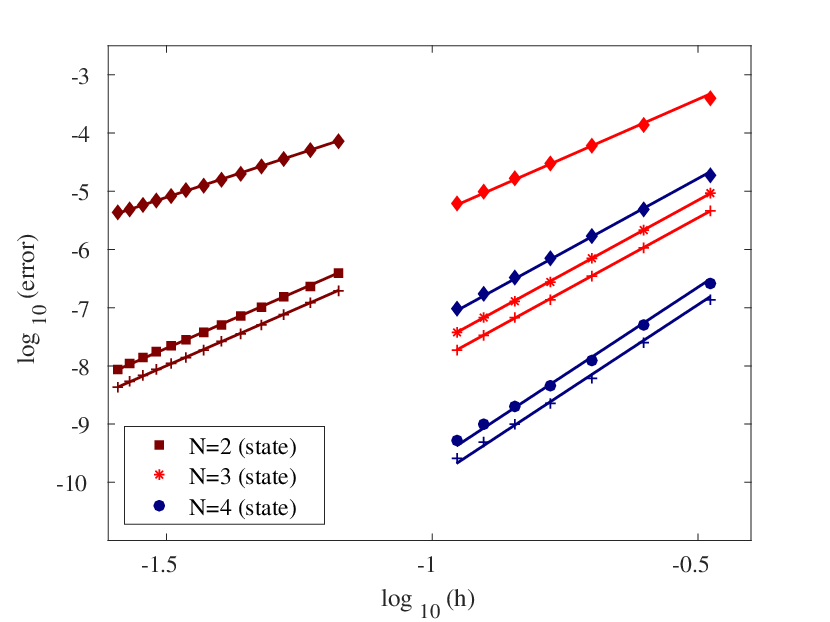
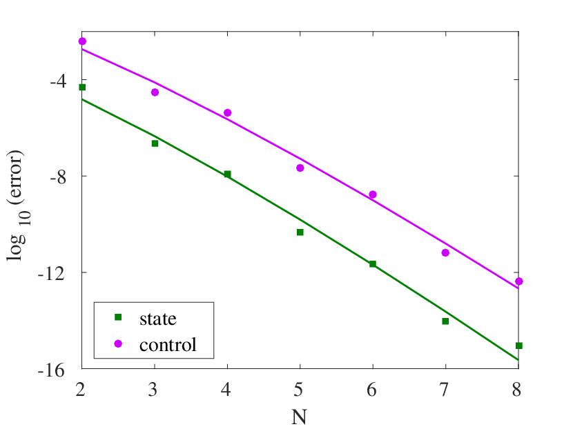
has a unique solution which depends Lipschitz continuously on the perturbation 𝐘{\bf{Y}}. This analysis, which utilizes assumptions (A1)–(A2) and properties (P1)–(P4), begins in Section 5 where perturbations in the linearized state and costate discrete dynamics are analyzed. In Section 6 it is shown that solving the linearized inclusion is equivalent to solving a quadratic program, where perturbations in the inclusion appear as linear terms in the quadratic program; the strong convexity assumption (A1) implies the existence of a unique solution to the quadratic program, which in turn implies the existence of a unique solution to the inclusion. Finally, in Section 7 the unique solution of the linearized inclusion is shown to depend Lipschitz continuously on the perturbation. This Lipschitz property and the bound for d∗d^{*} are combined with Proposition 3 to obtain (15). The tightness and possible extensions of the error bound (15) are explored in Section 8 using some problems with known solutions. In the proof of Theorem 1, we need to make the right side of (15) sufficiently small to establish the existence of the claimed solution to the discrete problem. The conditions η≥2\eta\geq 2 and N≥2N\geq 2 in the statement of the theorem ensure that as hh goes to zero, hp−1h^{p-1} and hq−1h^{q-1} go to zero, and as NN tends to infinity, (c/N)p−1(c/N)^{p-1} and (c/N)q−1.5(c/N)^{q-1.5} go to zero.

Since the discrete costate could be discontinuous across a mesh point, Theorem 1 implies convergence of the discrete costate on either side of the mesh point to the continuous costate at the mesh point. The discrete problem provides an estimate for the optimal control at t=1t=1 in the continuous problem, but not at t=0t=0 since this is not a collocation point. Due to the strong convexity assumption (A1), an estimate for the discrete control at t=0t=0 can be obtained from the minimum principle (6) since the initial state is given, while we have an estimate for the associated costate at t=0t=0. Alternatively, polynomial interpolation could be used to obtain estimates for the optimal control at t=0t=0.

In a recent paper [34], where we analyze a Gauss collocation scheme on a single interval, p=q=min⁡(η,N+1)p=q=\min(\eta,N+1). The differences between Radau and Gauss collocation are due to the asymmetry of the Radau points, and the asymmetry in the Radau first-order optimality conditions; that is, for the Radau points, 𝝀k∈𝒫N−1n\bm{\lambda}_{k}\in{\cal{P}}_{N-1}^{n} while 𝐱k∈𝒫Nn{\bf{x}}_{k}\in{\cal{P}}_{N}^{n}.

Notation. We let Ω\Omega denote the interval [−1,1][-1,1], while Ω0\Omega_{0} is the interval [0,1][0,1]. Let 𝒫N{\cal{P}}_{N} denote the space of polynomials of degree at most NN, while 𝒫N0{\cal{P}}_{N}^{0} is the subspace consisting of polynomials in 𝒫N{\cal{P}}_{N} that vanish at t=−1t=-1 and t=1t=1. The meaning of the norm ∥⋅∥∞\|\cdot\|_{\infty} is based on context. If 𝐱∈𝒞0​(Ω){\bf{x}}\in{\cal{C}}^{0}(\Omega), then ‖𝐱‖∞\|{\bf{x}}\|_{\infty} denotes the maximum of |𝐱⁡(t)||{\bf{x}}(t)| over t∈[−1,1]t\in[-1,1], where |⋅||\cdot| is the Euclidean norm. For a vector 𝐯∈ℝm{\bf{v}}\in\mathbb{R}^{m}, ‖𝐯‖∞\|{\bf{v}}\|_{\infty} is the maximum of |vi||v_{i}| over 1≤i≤m1\leq i\leq m. If 𝐀∈ℝm×n{\bf{A}}\in\mathbb{R}^{m\times n}, then ‖𝐀‖∞\|{\bf{A}}\|_{\infty} is the largest absolute row sum (the matrix norm induced by the ℓ∞\ell_{\infty} vector norm). We let |𝐀||{\bf{A}}| denote the matrix norm induced by the Euclidean vector norm. Throughout the paper, the index kk is used for the mesh interval, while the indices ii and jj are associated with collocation points. If 𝐩∈ℝK​N​n{\bf{p}}\in\mathbb{R}^{KNn}, then 𝐩k{\bf{p}}_{k} for 1≤k≤K1\leq k\leq K refers to vector with components 𝐩k​j∈ℝn{\bf{p}}_{kj}\in\mathbb{R}^{n}, for 1≤j≤N1\leq j\leq N. The dimension of the identity matrix 𝐈{\bf{I}} is often clear from context; when necessary, the dimension of 𝐈{\bf{I}} is specified by a subscript. For example, 𝐈n{\bf{I}}_{n} is the nn by nn identity matrix. The gradient is denoted ∇\nabla, while ∇2\nabla^{2} denotes the Hessian; subscripts indicate the differentiation variables. Throughout the paper, cc is a generic constant which has different values in different equations. The value of cc is always independent of hh, NN, and η\eta. The vector 𝟏{\bf{1}} has all entries equal to one, while the vector 𝟎{\bf{0}} has all entries equal to zero; again, their dimension should be clear from context. If 𝐃{\bf{D}} is the differentiation matrix introduced in (11), then 𝐃j{\bf{D}}_{j} is the jj-th column of 𝐃{\bf{D}} and 𝐃i:j{\bf{D}}_{i:j} is the submatrix formed by columns ii through jj. We let ⊗\otimes denote the Kronecker product. If 𝐔∈ℝm×n{\bf{U}}\in\mathbb{R}^{m\times n} and 𝐕∈ℝp×q{\bf{V}}\in\mathbb{R}^{p\times q}, then 𝐔⊗𝐕{\bf{U}}\otimes{\bf{V}} is the m​pmp by n​qnq block matrix whose (i,j)(i,j) block is ui​j​𝐕u_{ij}{\bf{V}}. We let ℒ2​(Ω){\cal{L}}^{2}(\Omega) denote the usual space of square integrable functions on Ω\Omega, while ℋp​(Ω){\cal{H}}^{p}(\Omega) is the Sobolev space consisting of functions with square integrable derivatives through order pp. The seminorm in ℋp​(Ω){\cal{H}}^{p}(\Omega), corresponding to the ℒ2​(Ω){\cal{L}}^{2}(\Omega) norm of the pp-order derivatives, is denoted |⋅|ℋp​(Ω)|\cdot|_{{\cal{H}}^{p}(\Omega)}. The subspace of ℋ1​(Ω){\cal{H}}^{1}(\Omega) corresponding to functions that vanish at t=−1t=-1 and t=1t=1 is denoted ℋ01​(Ω){\cal{H}}_{0}^{1}(\Omega).

2 Abstract setting

Given a feasible point for the discrete problem (4), define 𝐗k​j=𝐱k​(τj){\bf{X}}_{kj}={\bf{x}}_{k}(\tau_{j}) and 𝐔k​i=𝐮k​i{\bf{U}}_{ki}={\bf{u}}_{ki}. As noted earlier, 𝐃{\bf{D}} is a differentiation matrix in the sense that

∑j=0NDi​j​𝐗k​j=𝐱˙k​(τi),1≤i≤N.\sum_{j=0}^{N}D_{ij}{\bf{X}}_{kj}=\dot{{\bf{x}}}_{k}(\tau_{i}),\quad 1\leq i\leq N.

Hence, the discrete problem (4) can be reformulated as

minimizeC⁡(𝐗K​N)subject to∑j=0NDi​j𝐗k​j=h𝐟(𝐗k​i,𝐔k​i),𝐔k​i∈𝒰,1≤i≤N,𝐗k​0=𝐗k−1,N,1≤k≤K,}\left.\begin{array}[]{cll}\mbox{minimize}&C({\bf{X}}_{KN})&\\ \mbox{subject to}&\sum_{j=0}^{N}D_{ij}{\bf{X}}_{kj}=h{\bf{f}}({\bf{X}}_{ki},{\bf{U}}_{ki}),\quad{\bf{U}}_{ki}\in{\cal{U}},&1\leq i\leq N,\\ &{\bf{X}}_{k0}={\bf{X}}_{k-1,N},&1\leq k\leq K,\end{array}\right\} (16)

where 𝐗0​N=𝐚{\bf{X}}_{0N}={\bf{a}}, the starting condition.

We introduce multipliers 𝝁k​i\bm{\mu}_{ki} associated with the constraints in (16) and write the Lagrangian as

ℒ⁡(𝝁,𝐗,𝐔)=\displaystyle\mathcal{L}({\bm{\mu}},{\bf X},{\bf U})=
C⁡(𝐗K​N)+∑k=1K∑i=1N⟨𝝁k​i,h​𝐟​(𝐗k​i,𝐔k​i)−∑j=0NDi​j​𝐗k​j⟩+∑k=1K⟨𝝁k​0,(𝐗k−1,N−𝐗k​0)⟩.\displaystyle C\left(\mathbf{X}_{KN}\right)+\sum_{k=1}^{K}\sum_{i=1}^{N}\left\langle\bm{\mu}_{ki},h{\bf f}({\bf X}_{ki},{\bf U}_{ki})-\sum_{j=0}^{N}{D}_{ij}{\bf X}_{kj}\right\rangle+\sum_{k=1}^{K}\left\langle{\bm{\mu}}_{k0},\left({\bf X}_{k-1,N}-{\bf X}_{k0}\right)\right\rangle.

The first-order optimality conditions for (16), often called the Karush-Kuhn-Tucker (KKT) conditions, lead to the following relations (we show the variable with which we differentiate the Lagrangian followed by the associated condition):

𝐗k​0\displaystyle{\bf{X}}_{k0}\; ⇒\displaystyle\Rightarrow ∑i=1NDi​0​𝝁k​i=−𝝁k​0,\displaystyle\sum_{i=1}^{N}{D}_{i0}{\bm{\mu}}_{ki}=-\bm{\mu}_{k0}, (17)
𝐗k​j\displaystyle{\bf{X}}_{kj}\; ⇒\displaystyle\Rightarrow ∑i=1NDi​j​𝝁k​i=h​∇xH​(𝐗k​j,𝐔k​j,𝝁k​j),1≤j<N,\displaystyle\sum_{i=1}^{N}{D}_{ij}\bm{\mu}_{ki}=h\nabla_{x}H({\bf X}_{kj},{\bf U}_{kj},\bm{\mu}_{kj}),\quad 1\leq j<N, (18)
𝐗k​N\displaystyle{\bf{X}}_{kN} ⇒\displaystyle\Rightarrow ∑i=1NDi​N​𝝁k​i=h​∇xH​(𝐗k​N,𝐔k​N,𝝁k​N)+𝝁k+1,0,\displaystyle\sum_{i=1}^{N}{D}_{iN}{\bm{\mu}}_{ki}=h\nabla_{x}H({\bf X}_{kN},{\bf U}_{kN},\bm{\mu}_{kN})+\bm{\mu}_{k+1,0}, (19)
𝝁K+1,0:=∇C​(𝐗K​N),\displaystyle\quad\quad\bm{\mu}_{K+1,0}:=\nabla C({\bf{X}}_{KN}), (20)
𝐔k​i\displaystyle{\bf{U}}_{ki}\; ⇒\displaystyle\Rightarrow −∇uH​(𝐗k​i,𝐔k​i,𝝁k​i)∈N𝒰​(𝐔k​i).\displaystyle-\nabla_{u}H\left({\bf X}_{ki},{\bf U}_{ki},{\bm{\mu}}_{ki}\right)\in N_{{\cal{U}}}({\bf{U}}_{ki}). (21)

We first relate the KKT multipliers in (17)–(21) to the polynomials satisfying (7)–(9).

Proposition 2.

The multipliers 𝛍k∈ℝN​n\bm{\mu}_{k}\in\mathbb{R}^{Nn} satisfy (17)(\ref{NC0})–(21)(\ref{NC3}) if and only if the polynomial 𝛌k∈𝒫N−1n\bm{\lambda}_{k}\in{\cal{P}}_{N-1}^{n} given by 𝛌k​(τi)=𝛍k​i/ωi\bm{\lambda}_{k}(\tau_{i})=\bm{\mu}_{ki}/\omega_{i}, 1≤i≤N1\leq i\leq N, satisfies (7)(\ref{dcostate})–(9)(\ref{dcontrolmin}). Moreover, 𝛍k​0=𝛌k​(−1)\bm{\mu}_{k0}=\bm{\lambda}_{k}(-1).

Proof.

We start with multipliers 𝝁k\bm{\mu}_{k} satisfying (17)–(21). Define 𝚲k​i=𝝁k​i/ωi\bm{\Lambda}_{ki}=\bm{\mu}_{ki}/\omega_{i} for 1≤i≤N1\leq i\leq N, and let 𝝀k∈𝒫N−1n\bm{\lambda}_{k}\in{\cal{P}}_{N-1}^{n} be the polynomial that satisfies 𝝀k​(τi)=𝚲k​i\bm{\lambda}_{k}(\tau_{i})=\bm{\Lambda}_{ki}. Also, set 𝚲k​0=𝝁k​0\bm{\Lambda}_{k0}=\bm{\mu}_{k0}. In terms of 𝚲k​i\bm{\Lambda}_{ki} and the matrix Di​j‡=−ωjDj​i/ωiD_{ij}^{\ddagger}=-\omega_{j}D_{ji}/\omega_{i}, the equations (18), (19), and (21) become

∑j=1NDi​j‡​𝚲k​j\displaystyle\sum_{j=1}^{N}{D}_{ij}^{\ddagger}\bm{\Lambda}_{kj} =\displaystyle= −h​∇xH​(𝐗k​i,𝐔k​i,𝚲k​i),1≤i<N,\displaystyle-h\nabla_{x}H({\bf X}_{ki},{\bf U}_{ki},\bm{\Lambda}_{ki}),\quad 1\leq i<N, (22)
∑i=1NDN​i‡​𝚲k​i\displaystyle\sum_{i=1}^{N}{D}_{Ni}^{\ddagger}{\bm{\Lambda}}_{ki} =\displaystyle= −[h​∇xH​(𝐗k​N,𝐔k​N,𝚲k​N)+𝚲k+1,0/ωN],\displaystyle-[h\nabla_{x}H({\bf X}_{kN},{\bf U}_{kN},\bm{\Lambda}_{kN})+\bm{\Lambda}_{k+1,0}/\omega_{N}], (23)
N𝒰​(𝐔k​i)\displaystyle N_{{\cal{U}}}({\bf{U}}_{ki}) ∋\displaystyle\ni −∇uH​(𝐗k​i,𝐔k​i,𝚲k​i),1≤i≤N.\displaystyle-\nabla_{u}H({\bf X}_{ki},{\bf U}_{ki},\bm{\Lambda}_{ki}),\quad 1\leq i\leq N. (24)

Since the polynomial that is identically equal to 𝟏{\bf{1}} has derivative 𝟎{\bf{0}} and since 𝐃{\bf{D}} is a differentiation matrix, we have 𝐃𝟏=𝟎{\bf{D1}}={\bf{0}}, which implies that 𝐃0=−∑j=1N𝐃j{\bf D}_{0}=-\sum_{j=1}^{N}{\bf D}_{j}, where 𝐃j{\bf{D}}_{j} is the jj-th column of 𝐃{\bf{D}}. Hence, the first definition in (17) can be written

𝚲k​0\displaystyle\bm{\Lambda}_{k0} =\displaystyle= −∑i=1N𝝁k​iDi​0=∑i=1N∑j=1N𝝁k​iDi​j=∑i=1N∑j=1Nωj(𝝁k​iωi)(ωiDi​j/ωj)\displaystyle-\sum_{i=1}^{N}\bm{\mu}_{ki}D_{i0}=\sum_{i=1}^{N}\sum_{j=1}^{N}\bm{\mu}_{ki}D_{ij}=\sum_{i=1}^{N}\sum_{j=1}^{N}\omega_{j}\left(\frac{\bm{\mu}_{ki}}{\omega_{i}}\right)(\omega_{i}D_{ij}/\omega_{j}) (25)
=\displaystyle= −∑i=1N∑j=1NωiDi​j‡𝚲k​j\displaystyle-\sum_{i=1}^{N}\sum_{j=1}^{N}\omega_{i}D_{ij}^{\ddagger}\bm{\Lambda}_{kj}
=\displaystyle= 𝚲k+1,0+h​∑i=1Nωi​∇xH​(𝐗k​i,𝐔k​i,𝚲k​i),\displaystyle\bm{\Lambda}_{k+1,0}+h\sum_{i=1}^{N}\omega_{i}\nabla_{x}H({\bf{X}}_{ki},{\bf{U}}_{ki},\bm{\Lambda}_{ki}), (26)

where (26) is due to (22)–(23).

As noted in (13),

∑j=1NDi​j‡​𝚲k​j\displaystyle\sum_{j=1}^{N}D_{ij}^{\ddagger}\bm{\Lambda}_{kj} =\displaystyle= 𝝀˙k​(τi),1≤i<N,and\displaystyle\dot{\bm{\lambda}}_{k}(\tau_{i}),\quad 1\leq i<N,\quad\mbox{and} (27)
∑j=1NDN​j‡​𝚲k​j\displaystyle\sum_{j=1}^{N}D_{Nj}^{\ddagger}\bm{\Lambda}_{kj} =\displaystyle= 𝝀˙k​(1)−𝝀k​(1)/ωN.\displaystyle\dot{\bm{\lambda}}_{k}(1)-\bm{\lambda}_{k}(1)/\omega_{N}. (28)

This substitution in (25) yields

𝚲k​0=𝝀k​(1)−∑i=1Nωi​𝝀˙k​(τi).\bm{\Lambda}_{k0}=\bm{\lambda}_{k}(1)-\sum_{i=1}^{N}\omega_{i}\dot{\bm{\lambda}}_{k}(\tau_{i}). (29)

Since 𝝀˙k∈𝒫N−2n\dot{\bm{\lambda}}_{k}\in{\cal{P}}_{N-2}^{n} and NN-point Radau quadrature is exact for these polynomial, we have

∑i=1Nωi​𝝀˙k​(τi)=∫−11𝝀˙k​(τ)​𝑑τ=𝝀k​(1)−𝝀k​(−1).\sum_{i=1}^{N}\omega_{i}\dot{\bm{\lambda}}_{k}(\tau_{i})=\int_{-1}^{1}\dot{\bm{\lambda}}_{k}(\tau)d\tau=\bm{\lambda}_{k}(1)-\bm{\lambda}_{k}(-1). (30)

Combine (29) and (30) to obtain

𝚲k​0=𝝀k​(−1).\bm{\Lambda}_{k0}=\bm{\lambda}_{k}(-1). (31)

Let 𝐱k∈𝒫Nn{\bf{x}}_{k}\in{\cal{P}}_{N}^{n} be the polynomial that satisfies 𝐱k​(τj)=𝐗k​j{\bf{x}}_{k}(\tau_{j})={\bf{X}}_{kj} for all 0≤j≤N0\leq j\leq N. By (27), (7) is equivalent to (22) which is equivalent to (18) after a change of variables. By (28) and (31), (8) is equivalent to (23), which is equivalent to (19) after a change of variables. Finally, (9) is the same as (24) which is equivalent to (21) after a change of variables. The equivalence between 𝚲k​0\bm{\Lambda}_{k0} and 𝝀k​(−1)\bm{\lambda}_{k}(-1) was derived in (31). This shows that the polynomial 𝝀k​(τ)\bm{\lambda}_{k}(\tau) satisfies (7)–(9). The converse of the proposition follows by reversing all the steps in the derivation. ∎

The dynamics for (16), the first-order optimality conditions (22)–(24), the formula (26) for 𝚲k​0\bm{\Lambda}_{k0}, and the terminal costate condition (20) can be written as 𝒯⁡(𝐗,𝐔,𝚲)∈ℱ⁡(𝐔){\cal{T}}({\bf{X}},{\bf{U}},\bm{\Lambda})\in{\cal{F}}({\bf{U}}) where

𝒯1​k​i​(𝐗,𝐔,𝚲)\displaystyle{\cal{T}}_{1ki}({\bf{X}},{\bf{U}},\bm{\Lambda}) =\displaystyle= (∑j=0NDi​j​𝐗k​j)−h​𝐟​(𝐗k​i,𝐔k​i),1≤i≤N,\displaystyle\left(\sum_{j=0}^{N}{D}_{ij}{\bf X}_{kj}\right)-h{\bf f}({\bf X}_{ki},{\bf U}_{ki}),\quad 1\leq i\leq N, (32)
𝒯2​k​(𝐗,𝐔,𝚲)\displaystyle{\cal{T}}_{2k}({\bf{X}},{\bf{U}},\bm{\Lambda}) =\displaystyle= 𝐗k​0−𝐗k−1,N,\displaystyle{\bf X}_{k0}-{\bf{X}}_{k-1,N}, (33)
𝒯3​k​i​(𝐗,𝐔,𝚲)\displaystyle{\cal{T}}_{3ki}({\bf{X}},{\bf{U}},\bm{\Lambda}) =\displaystyle= (∑j=1NDi​j‡​𝚲k​j)+h​∇xH​(𝐗k​i,𝐔k​i,𝚲k​i),1≤i<N,\displaystyle\left(\sum_{j=1}^{N}{D}_{ij}^{\ddagger}{\bm{\Lambda}}_{kj}\right)+h\nabla_{x}H({\bf X}_{ki},{\bf U}_{ki},{\bm{\Lambda}}_{ki}),\quad 1\leq i<N, (34)
𝒯3​k​N​(𝐗,𝐔,𝚲)\displaystyle{\cal{T}}_{3kN}({\bf{X}},{\bf{U}},\bm{\Lambda}) =\displaystyle= ∑j=1NDN​j‡​𝚲k​j+h​∇xH​(𝐗k​N,𝐔k​N,𝚲k​N)+𝚲k+1,0/ωN,\displaystyle\sum_{j=1}^{N}{D}_{Nj}^{\ddagger}{\bm{\Lambda}}_{kj}+h\nabla_{x}H\left({{\bf{X}}}_{kN},{{\bf{U}}}_{kN},{\bm{\Lambda}}_{kN}\right)+\bm{\Lambda}_{k+1,0}/\omega_{N}, (35)
𝒯4​k​(𝐗,𝐔,𝚲)\displaystyle{\cal{T}}_{4k}({\bf{X}},{\bf{U}},\bm{\Lambda}) =\displaystyle= 𝚲k​0−𝚲k+1,0−h​∑i=1Nωi​∇xH​(𝐗k​i,𝐔k​i,𝚲k​i),\displaystyle\bm{\Lambda}_{k0}-\bm{\Lambda}_{k+1,0}-h\sum_{i=1}^{N}\omega_{i}\nabla_{x}H({\bf{X}}_{ki},{\bf{U}}_{ki},\bm{\Lambda}_{ki}), (36)
𝒯5​(𝐗,𝐔,𝚲)\displaystyle{\cal{T}}_{5}({\bf{X}},{\bf{U}},\bm{\Lambda}) =\displaystyle= ∇C​(𝐗K​N)−𝚲K+1,0,\displaystyle\nabla C({\bf{X}}_{KN})-\bm{\Lambda}_{K+1,0}, (37)
𝒯6​k​i​(𝐗,𝐔,𝚲)\displaystyle{\cal{T}}_{6ki}({\bf{X}},{\bf{U}},\bm{\Lambda}) =\displaystyle= −h​∇uH​(𝐗k​i,𝐔k​i,𝚲k​i),1≤i≤N,\displaystyle-h\nabla_{u}H({\bf X}_{ki},{\bf U}_{ki},{\bm{\Lambda}}_{ki}),\quad 1\leq i\leq N, (38)

where 1≤k≤K1\leq k\leq K. The initial state is 𝐗0​N=𝐗10=𝐚{\bf{X}}_{0N}={\bf{X}}_{10}={\bf{a}}. The components of ℱ{\cal{F}} are given by

ℱ1=ℱ2=ℱ3=ℱ4=ℱ5=𝟎,and ​ℱ6​k​i​(𝐔)=N𝒰​(𝐔k​i).{\cal{F}}_{1}={\cal{F}}_{2}={\cal{F}}_{3}={\cal{F}}_{4}={\cal{F}}_{5}={\bf{0}},\quad\mbox{and }{\cal{F}}_{6ki}({\bf{U}})=N_{\cal{U}}({\bf{U}}_{ki}).

The proof of Theorem 1 is based on [16, Proposition 3.1], given below in a slightly simplified form. Other results like this are contained in Theorem 3.1 of [15], in Proposition 5.1 of [29], in Theorem 2.1 of [30], and in Theorem 1 of [28].

Proposition 3.

Let 𝒳{\cal X} be a Banach space and let 𝒴{\cal Y} be a linear normed space with the norms in both spaces denoted ∥⋅∥\|\cdot\|. Let ℱ:𝒳↦2𝒴{\cal F}:{\cal X}\mapsto 2^{\cal Y} and let 𝒯:𝒳↦𝒴{\cal T}:{\cal X}\mapsto{\cal Y} with 𝒯\cal T continuously Fréchet differentiable in Br​(𝛉∗)B_{r}(\bm{\theta}^{*}), the ball with center 𝛉∗\bm{\theta}^{*} and radius rr, for some 𝛉∗∈𝒳\bm{\theta}^{*}\in{\cal X} and r>0r>0. Suppose that the following conditions hold for some 𝛅∈𝒴\bm{\delta}\in{\cal Y} and scalars ϵ\epsilon and γ>0\gamma>0:

  • (C1)

    𝒯⁡(𝜽∗)+𝜹∈ℱ⁡(𝜽∗){\cal T}(\bm{\theta}^{*})+\bm{\delta}\in{\cal F}(\bm{\theta}^{*}).

  • (C2)

    ‖∇𝒯​(𝜽)−∇𝒯​(𝜽∗)‖≤ϵ\|\nabla{\cal T}(\bm{\theta})-\nabla{\cal{T}}(\bm{\theta}^{*})\|\leq\epsilon for all 𝜽∈Br​(𝜽∗)\bm{\theta}\in B_{r}(\bm{\theta}^{*}).

  • (C3)

    The map (ℱ−∇𝒯​(𝜽∗))−1({\cal F}-\nabla{\cal{T}}(\bm{\theta}^{*}))^{-1} is single-valued and Lipschitz continuous with Lipschitz constant γ\gamma.

If ϵ​γ<1\epsilon\gamma<1 and ‖𝛅‖≤(1−γ​ϵ)​r/γ\|\bm{\delta}\|\leq(1-\gamma\epsilon)r/\gamma, then there exists a unique 𝛉∈Br​(𝛉∗)\bm{\theta}\in B_{r}(\bm{\theta}^{*}) such that 𝒯⁡(𝛉)∈ℱ⁡(𝛉){\cal T}(\bm{\theta})\in{\cal F}(\bm{\theta}). Moreover, we have the estimate

‖𝜽−𝜽∗‖≤γ1−γ​ϵ​‖𝜹‖.\|\bm{\theta}-\bm{\theta}^{*}\|\leq\frac{\gamma}{1-\gamma\epsilon}\|\bm{\delta}\|. (39)
Proof.

Define Φ⁡(𝜽)=\Phi(\bm{\theta})= [ℱ−∇𝒯​(𝜽∗)]−1​[𝒯−∇𝒯​(𝜽∗)]​(𝜽)[{\cal{F}}-\nabla{\cal{T}}(\bm{\theta}^{*})]^{-1}[{\cal{T}}-\nabla{\cal{T}}(\bm{\theta}^{*})](\bm{\theta}). For all 𝜽1\bm{\theta}_{1} and 𝜽2∈Br​(𝜽∗)\bm{\theta}_{2}\in B_{r}(\bm{\theta}^{*}), a Taylor expansion with integral remainder term yields

[𝒯−∇𝒯​(𝜽∗)]​(𝜽2)=[𝒯−∇𝒯​(𝜽∗)]​(𝜽1)+∫01[∇𝒯​(𝜽1+s⁡(𝜽2−𝜽1))−∇𝒯​(𝜽∗)]​𝑑s​(𝜽2−𝜽1).[{\cal{T}}-\nabla{\cal{T}}(\bm{\theta}^{*})](\bm{\theta}_{2})=[{\cal{T}}-\nabla{\cal{T}}(\bm{\theta}^{*})](\bm{\theta}_{1})+\int_{0}^{1}[\nabla{\cal{T}}(\bm{\theta}_{1}+s(\bm{\theta}_{2}-\bm{\theta}_{1}))-\nabla{\cal{T}}(\bm{\theta}^{*})]\;ds\;(\bm{\theta}_{2}-\bm{\theta}_{1}).

By (C2), it follows that

∥[𝒯−∇𝒯(𝜽∗)])(𝜽2)−[𝒯−∇𝒯(𝜽∗)](𝜽1)∥≤ϵ∥𝜽2−𝜽1∥.\|[{\cal{T}}-\nabla{\cal{T}}(\bm{\theta}^{*})])(\bm{\theta}_{2})-[{\cal{T}}-\nabla{\cal{T}}(\bm{\theta}^{*})](\bm{\theta}_{1})\|\leq\epsilon\|\bm{\theta}_{2}-\bm{\theta}_{1}\|. (40)

By (C3) and (40), we have

‖Φ⁡(𝜽1)−Φ⁡(𝜽2)‖\displaystyle\|\Phi(\bm{\theta}_{1})-\Phi(\bm{\theta}_{2})\|
=\displaystyle= ‖[ℱ−∇𝒯​(𝜽∗)]−1​[𝒯−∇𝒯​(𝜽∗)]​(𝜽1)−[ℱ−∇𝒯​(𝜽∗)]−1​[𝒯−∇𝒯​(𝜽∗)]​(𝜽2)‖\displaystyle\|[{\cal{F}}-\nabla{\cal{T}}(\bm{\theta}^{*})]^{-1}[{\cal{T}}-\nabla{\cal{T}}(\bm{\theta}^{*})](\bm{\theta}_{1})-[{\cal{F}}-\nabla{\cal{T}}(\bm{\theta}^{*})]^{-1}[{\cal{T}}-\nabla{\cal{T}}(\bm{\theta}^{*})](\bm{\theta}_{2})\|
≤\displaystyle\leq γ​‖[𝒯−∇𝒯​(𝜽∗)]​(𝜽1)−[𝒯−∇𝒯​(𝜽∗)]​(𝜽2)‖\displaystyle\gamma\|[{\cal{T}}-\nabla{\cal{T}}(\bm{\theta}^{*})](\bm{\theta}_{1})-[{\cal{T}}-\nabla{\cal{T}}(\bm{\theta}^{*})](\bm{\theta}_{2})\|
≤\displaystyle\leq ϵ​γ​‖𝜽1−𝜽2‖.\displaystyle\epsilon\gamma\|\bm{\theta}_{1}-\bm{\theta}_{2}\|.

Since ϵ​γ<1\epsilon\gamma<1, Φ\Phi is a contraction on Br​(𝜽∗)B_{r}(\bm{\theta}^{*}). Subtracting ∇𝒯​(𝜽∗)​(𝜽∗)\nabla{\cal{T}}(\bm{\theta}^{*})(\bm{\theta}^{*}) from each side of (C1) gives

[𝒯−∇𝒯​(𝜽∗)]​𝜽∗+𝜹∈[ℱ−∇𝒯​(𝜽∗)]​(𝜽∗),[{\cal{T}}-\nabla{\cal{T}}(\bm{\theta}^{*})]\bm{\theta}^{*}+\bm{\delta}\in[{\cal{F}}-\nabla{\cal{T}}(\bm{\theta}^{*})](\bm{\theta}^{*}),

and utilizing the uniqueness in (C3) yields

𝜽∗=[ℱ−∇𝒯​(𝜽∗)]−1​[(𝒯−∇𝒯​(𝜽∗))​𝜽∗+𝜹].\bm{\theta}^{*}=[{\cal{F}}-\nabla{\cal{T}}(\bm{\theta}^{*})]^{-1}[({\cal{T}}-\nabla{\cal{T}}(\bm{\theta}^{*}))\bm{\theta}^{*}+\bm{\delta}].

With this substitution, it follows from (40), (C3), and (C2) that

‖Φ⁡(𝜽)−𝜽∗‖\displaystyle\|\Phi(\bm{\theta})-\bm{\theta}^{*}\| (41)
=\displaystyle= ‖[ℱ−∇𝒯​(𝜽∗)]−1​[𝒯−∇𝒯​(𝜽∗)]​(𝜽)−[ℱ−∇𝒯​(𝜽∗)]−1​[(𝒯−∇𝒯​(𝜽∗))​(𝜽∗)+𝜹]‖\displaystyle\|[{\cal{F}}-\nabla{\cal{T}}(\bm{\theta}^{*})]^{-1}[{\cal{T}}-\nabla{\cal{T}}(\bm{\theta}^{*})](\bm{\theta})-[{\cal{F}}-\nabla{\cal{T}}(\bm{\theta}^{*})]^{-1}[({\cal{T}}-\nabla{\cal{T}}(\bm{\theta}^{*}))(\bm{\theta}^{*})+\bm{\delta}]\|
≤\displaystyle\leq γ∥[𝒯−∇𝒯(𝜽∗)](𝜽)−[𝒯−∇𝒯(𝜽∗)](𝜽∗)−𝜹]∥\displaystyle\gamma\|[{\cal{T}}-\nabla{\cal{T}}(\bm{\theta}^{*})](\bm{\theta})-[{\cal{T}}-\nabla{\cal{T}}(\bm{\theta}^{*})](\bm{\theta}^{*})-\bm{\delta}]\|
≤\displaystyle\leq γ⁡(ϵ​‖𝜽−𝜽∗‖+‖𝜹‖)≤γ⁡(ϵ​r+‖𝜹‖)\displaystyle\gamma(\epsilon\|\bm{\theta}-\bm{\theta}^{*}\|+\|\bm{\delta}\|)\leq\gamma(\epsilon r+\|\bm{\delta}\|)

for all 𝜽∈Br​(𝜽∗)\bm{\theta}\in B_{r}(\bm{\theta}^{*}). The assumption that ‖𝜹‖≤(1−γ​ϵ)​r/γ\|\bm{\delta}\|\leq(1-\gamma\epsilon)r/\gamma can be rearranged to obtain γ⁡(ϵ​r+‖𝜹‖)≤r\gamma(\epsilon r+\|\bm{\delta}\|)\leq r, which implies that ‖Φ⁡(𝜽)−𝜽∗‖≤r\|\Phi(\bm{\theta})-\bm{\theta}^{*}\|\leq r by (41). Since Φ\Phi maps Br​(𝜽∗)B_{r}(\bm{\theta}^{*}) into itself and Φ\Phi is a contraction on Br​(𝜽∗)B_{r}(\bm{\theta}^{*}), the contraction mapping principle yields the existence of a unique fixed point 𝜽∈Br​(𝜽∗)\bm{\theta}\in B_{r}(\bm{\theta}^{*}). Since ‖Φ⁡(𝜽)−𝜽∗‖=‖𝜽−𝜽∗‖\|\Phi(\bm{\theta})-\bm{\theta}^{*}\|=\|\bm{\theta}-\bm{\theta}^{*}\| for this fixed point, (39) is a consequence of (41). ∎

We use Proposition 3 with 𝜽∗=(𝐗∗,𝐔∗,𝚲∗)\bm{\theta}^{*}=({\bf{X}}^{*},{\bf{U}}^{*},\bm{\Lambda}^{*}) defined in (14) and 𝜽=(𝐗N,𝐔N,𝚲N)\bm{\theta}=({\bf{X}}^{N},{\bf{U}}^{N},\bm{\Lambda}^{N}). The norm on 𝒳{\cal{X}} is given by

‖𝜽‖=‖(𝐗,𝐔,𝚲)‖∞=max⁡{‖𝐗‖∞,‖𝐔‖∞,‖𝚲‖∞}.\|\bm{\theta}\|=\|({\bf X},{\bf U},{\bm{\Lambda}})\|_{\infty}=\max\{\|\bf X\|_{\infty},\|\bf U\|_{\infty},\|\bm{\Lambda}\|_{\infty}\}. (42)

The space 𝒴{\cal{Y}} corresponds to the codomain of 𝒯{\cal{T}}. If 𝐲∈𝒴{\bf{y}}\in{\cal{Y}}, then we let 𝐲l{\bf{y}}_{l} denote the part of 𝐲{\bf{y}} associated with 𝒯l{\cal{T}}_{l}, 1≤l≤61\leq l\leq 6. The norm of 𝐲∈𝒴{\bf{y}}\in{\cal{Y}} is given by

∥𝐲∥𝒴=∥𝐲1∥ω+|𝐲2|+∥𝐲3∥ω+|𝐲4|+h1/2|𝐲5|+h−1/2∥𝐲6∥∞,\|{\bf{y}}\|_{{\cal{Y}}}=\|{\bf{y}}_{1}\|_{\omega}+|{\bf{y}}_{2}|+\|{\bf{y}}_{3}\|_{\omega}+|{\bf{y}}_{4}|+h^{1/2}|{\bf{y}}_{5}|+h^{-1/2}\|{\bf{y}}_{6}\|_{\infty},

where for 𝐳∈ℝK​N​n{\bf{z}}\in\mathbb{R}^{KNn}, the ω\omega-norm is defined by

‖𝐳‖ω=(∑k=1K∑i=1Nωi​|𝐳k​i|2)1/2,𝐳k​i∈ℝn.\|{\bf{z}}\|_{\omega}=\left(\sum_{k=1}^{K}\sum_{i=1}^{N}\omega_{i}|{\bf{z}}_{ki}|^{2}\right)^{1/2},\quad{\bf{z}}_{ki}\in\mathbb{R}^{n}.

For 𝐳∈ℝN​n{\bf{z}}\in\mathbb{R}^{Nn}, the ω\omega-norm is

‖𝐳‖ω=(∑i=1Nωi​|𝐳i|2)1/2,𝐳i∈ℝn.\|{\bf{z}}\|_{\omega}=\left(\sum_{i=1}^{N}\omega_{i}|{\bf{z}}_{i}|^{2}\right)^{1/2},\quad{\bf{z}}_{i}\in\mathbb{R}^{n}.

3 Interpolation error in ℋ1{\cal{H}}^{1}

Our estimate for the distance from 𝒯⁡(𝐗∗,𝐔∗,𝚲∗){\cal{T}}({\bf{X}}^{*},{\bf{U}}^{*},\bm{\Lambda}^{*}) to ℱ⁡(𝐔∗){\cal{F}}({\bf{U}}^{*}) utilizes the following bound for the ℋ1​(Ω){\cal{H}}^{1}(\Omega) error of the interpolant based on the point set τi\tau_{i}, 0≤i≤N0\leq i\leq N.

Lemma 4.

If u∈ℋη​(Ω)u\in{\cal{H}}^{\eta}(\Omega) for some η≥2\eta\geq 2, then there exists a constant cc, independent of NN and η\eta, such that

|u−uI|ℋ1​(Ω)≤(c/N)p−1​|u|ℋp​(Ω),p=min⁡{η,N+1},|u-u^{I}|_{{\cal{H}}^{1}(\Omega)}\leq(c/N)^{p-1}|u|_{{\cal{H}}^{p}(\Omega)},\quad p=\min\{\eta,N+1\}, (43)

where uI∈𝒫Nu^{I}\in{\cal{P}}_{N} is the interpolant of uu satisfying uI​(τi)=u⁡(τi)u^{I}(\tau_{i})=u(\tau_{i}), 0≤i≤N0\leq i\leq N, and N>0N>0. In the case η=p=1\eta=p=1, there exists a constant cc, independent of NN, such that

|u−uI|ℋ1​(Ω)≤c​|u|ℋ1​(Ω),|u-u^{I}|_{{\cal{H}}^{1}(\Omega)}\leq c|u|_{{\cal{H}}^{1}(\Omega)}, (44)
Proof.

Throughout the analysis, cc denotes a generic constant whose value is independent of NN and η\eta, and which may have different values in different equations. We first show that if the lemma holds for all u∈ℋ01​(Ω)∩ℋη​(Ω)u\in{\cal{H}}_{0}^{1}(\Omega)\cap{\cal{H}}^{\eta}(\Omega), then it holds for all u∈ℋη​(Ω)u\in{\cal{H}}^{\eta}(\Omega). Suppose u∈ℋη​(Ω)u\in{\cal{H}}^{\eta}(\Omega) and let ℓ\ell denote the linear function for which ℓ⁡(±1)=u⁡(±1)\ell(\pm 1)=u(\pm 1). Since ℓI=ℓ\ell^{I}=\ell, it follows that

|u−uI|ℋ1​(Ω)=|(u−ℓ)−(u−ℓ)I|ℋ1​(Ω).|u-u^{I}|_{{\cal{H}}^{1}(\Omega)}=|(u-\ell)-(u-\ell)^{I}|_{{\cal{H}}^{1}(\Omega)}.

Since u−ℓ∈ℋ01​(Ω)u-\ell\in{\cal{H}}_{0}^{1}(\Omega), (43) gives

|u−uI|ℋ1​(Ω)≤(c/N)p−1​|u−ℓ|ℋp​(Ω)|u-u^{I}|_{{\cal{H}}^{1}(\Omega)}\leq(c/N)^{p-1}|u-\ell|_{{\cal{H}}^{p}(\Omega)}

when η≥2\eta\geq 2. Moreover, when η≥2\eta\geq 2, |u−ℓ|ℋp​(Ω)=|u|ℋp​(Ω)|u-\ell|_{{\cal{H}}^{p}(\Omega)}=|u|_{{\cal{H}}^{p}(\Omega)} since derivatives of order two or larger applied to the linear function ℓ\ell are zero. This establishes (43) for all u∈ℋη​(Ω)u\in{\cal{H}}^{\eta}(\Omega) with η≥2\eta\geq 2. If η=1\eta=1, then by (44), we have

|u−uI|ℋ1​(Ω)≤c​|u−ℓ|ℋ1​(Ω)≤c⁡(|u|ℋ1​(Ω)+(|ℓ|ℋ1​(Ω))CLOSE.|u-u^{I}|_{{\cal{H}}^{1}(\Omega)}\leq c|u-\ell|_{{\cal{H}}^{1}(\Omega)}\leq c\left(|u|_{{\cal{H}}^{1}(\Omega)}+(|\ell|_{{\cal{H}}^{1}(\Omega)}\right). (45)

Since ℓ˙=(u⁡(1)−u⁡(−1))/2\dot{\ell}=(u(1)-u(-1))/2, the Schwarz inequality gives

|ℓ|ℋ1​(Ω)=|u⁡(1)−u⁡(−1)|2=12​|∫−11u˙​(τ)​𝑑τ|≤|u|ℋ1​(Ω).|\ell|_{{\cal{H}}^{1}(\Omega)}=\frac{|u(1)-u(-1)|}{\sqrt{2}}=\frac{1}{\sqrt{2}}\left|\int_{-1}^{1}\dot{u}(\tau)\;d\tau\right|\leq|u|_{{\cal{H}}^{1}(\Omega)}. (46)

Combine (45) and (46) to obtain (44) for all u∈ℋ1​(Ω)u\in{\cal{H}}^{1}(\Omega). Henceforth, it is assumed that u∈ℋ01​(Ω)∩ℋη​(Ω)u\in{\cal{H}}_{0}^{1}(\Omega)\cap{\cal{H}}^{\eta}(\Omega).

Let πN​u\pi_{N}u denote the projection of uu into 𝒫N0{\cal{P}}_{N}^{0} relative to the norm |⋅|ℋ1​(Ω)|\cdot|_{{\cal{H}}^{1}(\Omega)}. Define EN=u−πN​uE_{N}=u-\pi_{N}u and eN=ENI=(u−πN​u)I=uI−πN​ue_{N}=E_{N}^{I}=(u-\pi_{N}u)^{I}=u^{I}-\pi_{N}u. Since EN−eN=u−uIE_{N}-e_{N}=u-u^{I}, it follows that

|u−uI|ℋ1​(Ω)≤|EN|ℋ1​(Ω)+|​eN|ℋ1​(Ω).|u-u^{I}|_{{\cal{H}}^{1}(\Omega)}\leq|E_{N}|_{{\cal{H}}^{1}(\Omega)}+|e_{N}|_{{\cal{H}}^{1}(\Omega)}. (47)

In [19, Prop. 3.1] it is shown that for η≥1\eta\geq 1,

|EN|ℋ1​(Ω)≤(c/N)p−1​|u|ℋp​(Ω),where ​p=min⁡{η,N+1}.|E_{N}|_{{\cal{H}}^{1}(\Omega)}\leq(c/N)^{p-1}|u|_{{\cal{H}}^{p}(\Omega)},\quad\mbox{where }p=\min\{\eta,N+1\}. (48)

We will establish the bound

|eN|ℋ1​(Ω)≤c​|EN|ℋ1​(Ω).|e_{N}|_{{\cal{H}}^{1}(\Omega)}\leq c|E_{N}|_{{\cal{H}}^{1}(\Omega)}. (49)

Combine (47)–(49) to obtain (43) and (44) for an appropriate choice of cc.

By [5, Lem. 4.4] and the fact that eN∈𝒫N0e_{N}\in{\cal{P}}_{N}^{0}, it follows that

|eN|ℋ1​(Ω)≤c​N​(∫ΩeN2​(τ)1−τ2​𝑑τ)1/2.|e_{N}|_{{\cal{H}}^{1}(\Omega)}\leq cN\left(\int_{\Omega}\frac{e_{N}^{2}(\tau)}{1-\tau^{2}}\;d\tau\right)^{1/2}. (50)

Since eN∈𝒫N0e_{N}\in{\cal{P}}_{N}^{0} and eN2​(τ)/(1−τ2)∈𝒫2​N−20e_{N}^{2}(\tau)/(1-\tau^{2})\in{\cal{P}}_{2N-2}^{0}, NN-point Radau quadrature is exact, and we have

(∫ΩeN2​(τ)1−τ2​𝑑τ)1/2=(∑i=1N−1ωi​eN2​(τi)1−τi2)1/2=(∑i=1N−1ωi​EN2​(τi)1−τi2)1/2.\left(\int_{\Omega}\frac{e_{N}^{2}(\tau)}{1-\tau^{2}}\;d\tau\right)^{1/2}=\left(\sum_{i=1}^{N-1}\frac{\omega_{i}e_{N}^{2}(\tau_{i})}{1-\tau_{i}^{2}}\right)^{1/2}=\left(\sum_{i=1}^{N-1}\frac{\omega_{i}E_{N}^{2}(\tau_{i})}{1-\tau_{i}^{2}}\right)^{1/2}. (51)

The last equality holds since eN=ENe_{N}=E_{N} at τi\tau_{i}, 0≤i≤N0\leq i\leq N. Although Lemma 4.3 in [5] was given for Lobatto quadrature, exactly the same proof can be used for both Gauss and Radau quadrature. Consequently, since EN∈ℋ01​(Ω)E_{N}\in{\cal{H}}_{0}^{1}(\Omega), it follows from [5, Lem. 4.3] that

(∑i=1Nωi​EN2​(τi)1−τi2)1/2≤c⁡[(∫ΩEN2​(τ)1−τ2​𝑑τ)1/2+N−1​|EN|ℋ1​(Ω)].\left(\sum_{i=1}^{N}\frac{\omega_{i}E_{N}^{2}(\tau_{i})}{1-\tau_{i}^{2}}\right)^{1/2}\leq c\left[\left(\int_{\Omega}\frac{E_{N}^{2}(\tau)}{1-\tau^{2}}\;d\tau\right)^{1/2}+N^{-1}|E_{N}|_{{\cal{H}}^{1}(\Omega)}\right]. (52)

By [34, Prop. 9.1], we have

N⁡[(∫ΩEN2​(τ)1−τ2​𝑑τ)1/2+N−1|EN|ℋ1​(Ω)]≤2|EN|ℋ1​(Ω).N\left[\left(\int_{\Omega}\frac{E_{N}^{2}(\tau)}{1-\tau^{2}}\;d\tau\right)^{1/2}+N^{-1}|E_{N}|_{{\cal{H}}^{1}(\Omega)}\right]\leq 2|E_{N}|_{{\cal{H}}^{1}(\Omega)}. (53)

Combine (50–53) to obtain (49). ∎

Remark 3.1.

In the analogue of Lemma 4 for the Gauss quadrature points given in [34, Lem. 4.1], the exponent in the error bound is p−1.5p-1.5 instead of p−1p-1. The difference in the exponent is due to the treatment of endpoints. In the Radau result, the polynomial interpolates at both τ=−1\tau=-1 and τ=1\tau=1, while in the Gauss result, the polynomial interpolates only at τ=−1\tau=-1.

4 Analysis of the residual

The distance from 𝒯⁡(𝐗∗,𝐔∗,𝚲∗){\cal{T}}({\bf{X}}^{*},{\bf{U}}^{*},\bm{\Lambda}^{*}) to ℱ⁡(𝐔∗){\cal{F}}({\bf{U}}^{*}) is now estimated.

Lemma 5.

If 𝐱∗{\bf{x}}^{*} and 𝛌∗∈𝒫ℋη​(Ω0)\bm{\lambda}^{*}\in{\cal{PH}}^{\eta}(\Omega_{0}) for some η≥2\eta\geq 2, then there exists a constant cc, independent of NN, hh, and η\eta, such that

dist​[𝒯⁡(𝐗∗,𝐔∗,𝚲∗),ℱ⁡(𝐔∗)]𝒴\displaystyle{\rm dist}[{\cal{T}}({\bf{X}}^{*},{\bf{U}}^{*},\bm{\Lambda}^{*}),{\cal{F}}({\bf{U}}^{*})]_{{\cal{Y}}}
≤hp−1/2​(cN)p−1​|𝐱∗|𝒫ℋp​(Ω0)+hq−1/2​(cN)q−1.5|​𝝀∗|𝒫ℋq​(Ω0),\displaystyle\leq h^{p-1/2}\left(\frac{c}{N}\right)^{p-1}|{\mathbf{x}^{*}}|_{{\cal{PH}}^{p}(\Omega_{0})}+h^{q-1/2}\left(\frac{c}{N}\right)^{q-1.5}|{\mbox{\boldmath$\lambda$}^{*}}|_{{\cal{PH}}^{q}(\Omega_{0})}, (54)

where p=min⁡(η,N+1)p=\min(\eta,N+1) and q=min⁡(η,N)q=\min(\eta,N).

Proof.

Since 𝒯⁡(𝐗∗,𝐔∗,𝚲∗){\cal{T}}({\bf{X}}^{*},{\bf{U}}^{*},\bm{\Lambda}^{*}) appears throughout the analysis, it is abbreviated 𝒯∗{\cal{T}}^{*}. Since the minimum principle (6) holds for all t∈Ω0t\in\Omega_{0}, it holds at the collocation points, which implies that 𝒯6∗∈ℱ6​(𝐔∗){\cal{T}}_{6}^{*}\in{\cal{F}}_{6}({\bf{U}}^{*}). Also, 𝒯2∗=𝒯5∗=𝟎{\cal{T}}_{2}^{*}={\cal{T}}_{5}^{*}={\bf{0}} since the optimal state is continuous and it satisfies the terminal condition (5) in the costate equation. Thus we only need to analyze 𝒯1∗{\cal{T}}_{1}^{*}, 𝒯3∗{\cal{T}}_{3}^{*}, and 𝒯4∗{\cal{T}}_{4}^{*}.

Let us first consider 𝒯1∗\mathcal{T}_{1}^{*}. Since 𝐃{\bf D} is a differentiation matrix associated with the collocation points, we have

∑j=0NDi​j​𝐗k​j∗=𝐱˙kI​(τi),1≤i≤N,\sum_{j=0}^{N}D_{ij}{\bf X}_{kj}^{*}=\dot{\bf x}_{k}^{I}(\tau_{i}),\quad 1\leq i\leq N, (55)

where 𝐱kI∈𝒫Nn{\bf x}_{k}^{I}\in\mathcal{P}_{N}^{n} is the (interpolating) polynomial that passes through 𝐱k∗​(τj){\bf x}_{k}^{*}(\tau_{j}) for 0≤j≤N0\leq j\leq N. Since 𝐱∗{\bf x}^{*} satisfies the dynamics of (1),

h​𝐟​(𝐗k​i∗,𝐔k​i∗)=𝐱˙k∗​(τi).h{\bf f}({\bf X}_{ki}^{*},{\bf U}_{ki}^{*})=\dot{\bf x}_{k}^{*}(\tau_{i}). (56)

Combine (55) and (56) to obtain

𝒯1​k​i∗=𝐱˙kI​(τi)−𝐱˙k∗​(τi)=𝐱˙kI​(τi)−(𝐱˙k∗)J​(τi),\mathcal{T}_{1ki}^{*}=\dot{\bf x}_{k}^{I}(\tau_{i})-\dot{\bf x}_{k}^{*}(\tau_{i})=\dot{\bf x}_{k}^{I}(\tau_{i})-(\dot{\bf x}_{k}^{*})^{J}(\tau_{i}), (57)

where (𝐱˙k∗)J∈𝒫N−1n(\dot{{\bf{x}}}_{k}^{*})^{J}\in{\cal{P}}_{N-1}^{n} is the interpolant that passes through 𝐱˙k∗​(τi)\dot{\bf x}_{k}^{*}(\tau_{i}) for 1≤i≤N1\leq i\leq N. Since both 𝐱˙I\dot{\bf x}^{I} and (𝐱˙∗)J(\dot{{\bf{x}}}^{*})^{J} are polynomials of degree N−1N-1 and Radau quadrature is exact for polynomials of degree 2​N−22N-2, it follows that

‖𝒯1∗‖ω2\displaystyle\|{\cal{T}}_{1}^{*}\|_{\omega}^{2} =\displaystyle= ∑k=1K∑i=1Nωi​|𝐱˙kI​(τi)−(𝐱˙k∗)J​(τi)|2\displaystyle\sum_{k=1}^{K}\sum_{i=1}^{N}\omega_{i}|\dot{\bf x}_{k}^{I}(\tau_{i})-(\dot{\bf x}_{k}^{*})^{J}(\tau_{i})|^{2} (58)
=\displaystyle= ∑k=1K∫−11|𝐱˙kI​(τ)−(𝐱˙k∗)J​(τ)|2​𝑑τ\displaystyle\sum_{k=1}^{K}\int_{-1}^{1}|\dot{\bf x}_{k}^{I}(\tau)-(\dot{\bf x}_{k}^{*})^{J}(\tau)|^{2}\;d\tau
≤\displaystyle\leq 2​∑k=1K∫−11(|𝐱˙kI​(τ)−𝐱˙k∗​(τ)|2+|𝐱˙k∗​(τ)−(𝐱˙k∗)J​(τ)|2)​𝑑τ.\displaystyle 2\sum_{k=1}^{K}\int_{-1}^{1}\left(|\dot{\bf x}_{k}^{I}(\tau)-\dot{\bf x}_{k}^{*}(\tau)|^{2}+|\dot{\bf x}_{k}^{*}(\tau)-(\dot{\bf x}_{k}^{*})^{J}(\tau)|^{2}\right)\;d\tau.

By Lemma 4, we have

‖𝐱˙kI−𝐱˙k∗‖ℒ2​(Ω)≤(c/N)p−1​|𝐱k∗|ℋp​(Ω),p=min⁡{η,N+1}.\|\dot{\bf x}_{k}^{I}-\dot{\bf x}_{k}^{*}\|_{{\cal{L}}^{2}(\Omega)}\leq(c/N)^{p-1}|{\bf{x}}^{*}_{k}|_{{\cal{H}}^{p}(\Omega)},\quad p=\min\{\eta,N+1\}. (59)

The second term in (58) involves the difference between between 𝐱˙k∗∈ℋ(η−1)\dot{{\bf{x}}}_{k}^{*}\in{\cal{H}}^{(\eta-1)} and its interpolant (𝐱˙k∗)J∈𝒫N−1n(\dot{\bf x}_{k}^{*})^{J}\in{\cal{P}}_{N-1}^{n} at the NN Radau points. By the bound given in [9, (5.4.33)] for the ℒ2{\cal{L}}^{2} error in Radau interpolation, this term has exactly the same bound as that on the right side of (59). Since 𝐱k​(τ)=𝐱⁡(tk−1/2+h​τ){\bf{x}}_{k}(\tau)={\bf{x}}(t_{k-1/2}+h\tau), the derivatives contained in the right side of (59) satisfy

dp​𝐱k∗​(τ)d​τp=hp​dp​𝐱∗​(t)d​tp|t=tk−1/2+h​τ.\frac{d^{p}{\bf{x}}_{k}^{*}(\tau)}{d\tau^{p}}=h^{p}\left.\frac{d^{p}{\bf{x}}^{*}(t)}{dt^{p}}\right|_{t=t_{k-1/2}+h\tau}.

Consequently, after a change of variables, we have

∫−11|dp​𝐱k∗​(τ)d​τp|2​𝑑τ=h2​p−1​∫tk−1tk|dp​𝐱∗​(t)d​tp|2​𝑑t.\int_{-1}^{1}\left|\frac{d^{p}{\bf{x}}_{k}^{*}(\tau)}{d\tau^{p}}\right|^{2}\;d\tau=h^{2p-1}\int_{t_{k-1}}^{t_{k}}\left|\frac{d^{p}{\bf{x}}^{*}(t)}{dt^{p}}\right|^{2}\;dt.

Combine this with (58) and (59) to deduce that ‖𝒯1∗‖ω\|{\cal{T}}^{*}_{1}\|_{\omega} is bounded by the first term on the right side side of (54).

The analysis of 𝒯3∗{\cal{T}}_{3}^{*} is similar to the analysis of 𝒯1∗{\cal{T}}_{1}^{*}. Let 𝝀kI∈𝒫N−1n\bm{\lambda}_{k}^{I}\in{\cal{P}}_{N-1}^{n} be the polynomial that interpolates 𝝀k∗​(τj)\bm{\lambda}_{k}^{*}(\tau_{j}) for 1≤j≤N1\leq j\leq N. By (27) and (28), we have

∑j=1NDi​j‡​𝚲k​j∗\displaystyle\sum_{j=1}^{N}D_{ij}^{\ddagger}\bm{\Lambda}_{kj}^{*} =\displaystyle= 𝝀˙kI​(τi),1≤i<N,\displaystyle\dot{\bm{\lambda}}_{k}^{I}(\tau_{i}),\quad 1\leq i<N, (60)
∑j=1NDN​j‡​𝚲k​j∗\displaystyle\sum_{j=1}^{N}D_{Nj}^{\ddagger}\bm{\Lambda}_{kj}^{*} =\displaystyle= 𝝀˙kI​(τi)−𝝀k∗​(1)/ωN.\displaystyle\dot{\bm{\lambda}}_{k}^{I}(\tau_{i})-\bm{\lambda}_{k}^{*}(1)/\omega_{N}. (61)

Since 𝝀∗\bm{\lambda}^{*} satisfies (5), it follows that

h​∇xH​(𝐗k​i∗,𝐔k​i∗,𝚲k​i∗)=h​∇xH​(𝐱k∗​(τi),𝐮k∗​(τi),𝝀k∗​(τi))=−𝝀˙k∗​(τi),h\nabla_{x}H({\bf X}_{ki}^{*},{\bf U}_{ki}^{*},{\bm{\Lambda}}_{ki}^{*})=h\nabla_{x}H({\bf x}_{k}^{*}(\tau_{i}),{\bf u}_{k}^{*}(\tau_{i}),{\bm{\lambda}}_{k}^{*}(\tau_{i}))=-\dot{\bm{\lambda}}_{k}^{*}(\tau_{i}), (62)

1≤i≤N1\leq i\leq N. We substitute (60)–(62) in the definition of 𝒯3{\cal{T}}_{3} to obtain

𝒯3​k​i​(𝐗∗,𝐔∗,𝚲∗)=𝝀˙kI​(τi)−𝝀˙k∗​(τi)=𝝀˙kI​(τi)−(𝝀˙k∗)J​(τi),1≤i≤N,{\cal{T}}_{3ki}({\bf{X}}^{*},{\bf{U}}^{*},\bm{\Lambda}^{*})=\dot{\bm{\lambda}}_{k}^{I}(\tau_{i})-\dot{\bm{\lambda}}_{k}^{*}(\tau_{i})=\dot{\bm{\lambda}}_{k}^{I}(\tau_{i})-(\dot{\bm{\lambda}}_{k}^{*})^{J}(\tau_{i}),\quad 1\leq i\leq N,

where (𝝀˙k∗)J∈𝒫N−1n(\dot{\bm{\lambda}}_{k}^{*})^{J}\in{\cal{P}}_{N-1}^{n} is the polynomial that passes through 𝝀˙k∗​(τi)\dot{\bm{\lambda}}_{k}^{*}(\tau_{i}), 1≤i≤N1\leq i\leq N. Note that the term −𝝀k∗(1)/ωN-\bm{\lambda}_{k}^{*}(1)/\omega_{N} in (61) cancels the corresponding term in 𝒯3​k{\cal{T}}_{3k} due to the continuity of 𝝀∗\bm{\lambda}^{*}. Since 𝝀˙kI∈𝒫N−2n\dot{\bm{\lambda}}_{k}^{I}\in{\cal{P}}_{N-2}^{n} and (𝝀˙k∗)J∈𝒫N−1n(\dot{\bm{\lambda}}_{k}^{*})^{J}\in{\cal{P}}_{N-1}^{n}, and since Radau quadrature is exact for polynomials of degree 2​N−22N-2, we obtain, as in (58),

‖𝒯3∗‖ω2≤2​∑k=1K∫−11(|𝝀˙kI​(τ)−𝝀˙k∗​(τ)|2+|𝝀˙k∗​(τ)−(𝝀˙k∗)J​(τ)|2)​𝑑τ.\|{\cal{T}}_{3}^{*}\|_{\omega}^{2}\leq 2\sum_{k=1}^{K}\int_{-1}^{1}\left(|\dot{\bm{\lambda}}_{k}^{I}(\tau)-\dot{\bm{\lambda}}_{k}^{*}(\tau)|^{2}+|\dot{\bm{\lambda}}_{k}^{*}(\tau)-(\dot{\bm{\lambda}}_{k}^{*})^{J}(\tau)|^{2}\right)\;d\tau. (63)

The last term in (63) has the bound

‖(𝝀˙k∗)J−𝝀˙k∗‖ℒ2​(Ω)≤hp​(c/N)p−1​|𝝀∗|ℋp​(tk−1,tk),p=min⁡{η,N+1},\|(\dot{\bm{\lambda}}^{*}_{k})^{J}-\dot{\bm{\lambda}}_{k}^{*}\|_{{\cal{L}}^{2}(\Omega)}\leq h^{p}(c/N)^{p-1}|\bm{\lambda}^{*}|_{{\cal{H}}^{p}(t_{k-1},t_{k})},\quad p=\min\{\eta,N+1\}, (64)

corresponding to the ℒ2{\cal{L}}^{2} error in interpolation at the Radau points. The other term, however, is different from the state since 𝝀kI\bm{\lambda}_{k}^{I} has degree N−1N-1 while the state 𝐱kI{\bf{x}}_{k}^{I} has degree NN, and the state interpolates at both the quadrature points and at τ=−1\tau=-1, while 𝝀kI\bm{\lambda}_{k}^{I} only interpolates at the quadrature points. The error in the derivative of the interpolant at the Radau points has the bound [9, (5.4.34)]

‖𝝀˙kI−𝝀˙k∗‖ℒ2​(Ω)≤hq​(c/N)q−1.5​|𝝀∗|ℋq​(Ω),q=min⁡{η,N}.\|\dot{\bm{\lambda}}_{k}^{I}-\dot{\bm{\lambda}}_{k}^{*}\|_{{\cal{L}}^{2}(\Omega)}\leq h^{q}(c/N)^{q-1.5}|\bm{\lambda}^{*}|_{{\cal{H}}^{q}(\Omega)},\quad q=\min\{\eta,N\}. (65)

The exponent changes from p−1p-1 in (64) to q−1.5q-1.5 due to the fact that 𝝀kI\bm{\lambda}_{k}^{I} does not interpolate at τ=−1\tau=-1, and q≤pq\leq p since the polynomial associated with 𝝀kI\bm{\lambda}_{k}^{I} has degree N−1N-1. Note that if 𝝀∗∈𝒫ℋη​(Ω0)\bm{\lambda}^{*}\in{\cal{PH}}^{\eta}(\Omega_{0}), then 𝝀∗∈𝒫ℋ(η−1)​(Ω0)\bm{\lambda}^{*}\in{\cal{PH}}^{(\eta-1)}(\Omega_{0}), so we can always ensure that the error bound (65) dominates the error bound (64) by lowering η\eta in (64) if necessary. Utilizing the bound (65) in (63) and changing variables from τ\tau to tt, we deduce that ‖𝒯3‖ω\|{\cal{T}}_{3}\|_{\omega} is bounded by the second term on the right side of (54).

Finally, let us consider 𝒯4∗{\cal{T}}_{4}^{*}. Applying (62) and utilizing the continuity of 𝝀∗\bm{\lambda}^{*} and the exactness of Radau quadrature, we have

𝒯4​k∗\displaystyle{\cal{T}}_{4k}^{*} =\displaystyle= 𝝀k∗​(−1)−𝝀k+1∗​(−1)+∑i=1Nωi​𝝀˙k∗​(τi)\displaystyle{\bm{\lambda}}_{k}^{*}(-1)-{\bm{\lambda}}_{k+1}^{*}(-1)+\sum_{i=1}^{N}\omega_{i}\dot{\bm{\lambda}}_{k}^{*}(\tau_{i})
=\displaystyle= 𝝀k∗​(−1)−𝝀k∗​(1)+∑i=1Nωi​(𝝀˙k∗)J​(τi)\displaystyle{\bm{\lambda}}_{k}^{*}(-1)-{\bm{\lambda}}_{k}^{*}(1)+\sum_{i=1}^{N}\omega_{i}(\dot{\bm{\lambda}}_{k}^{*})^{J}(\tau_{i})
=\displaystyle= 𝝀k∗​(−1)−𝝀k∗​(1)+∫−11(𝝀˙k∗)J​(τ)​𝑑τ=∫−11[(𝝀˙k∗)J​(τ)−𝝀˙k∗​(τ)]​𝑑τ.\displaystyle{\bm{\lambda}}_{k}^{*}(-1)-{\bm{\lambda}}_{k}^{*}(1)+\int_{-1}^{1}(\dot{\bm{\lambda}}_{k}^{*})^{J}(\tau)\;d\tau=\int_{-1}^{1}[(\dot{\bm{\lambda}}_{k}^{*})^{J}(\tau)-\dot{\bm{\lambda}}_{k}^{*}(\tau)]\;d\tau.

By (64) and the Schwarz inequality, we have

|𝒯4​k∗|≤2​‖(𝝀˙k∗)J−𝝀˙k∗‖ℒ2​(Ω)≤hp​(c/N)p−1​|𝝀∗|ℋp​(Ω),p=min⁡{η,N+1}.|{\cal{T}}_{4k}^{*}|\leq\sqrt{2}\|(\dot{\bm{\lambda}}_{k}^{*})^{J}-\dot{\bm{\lambda}}_{k}^{*}\|_{{\cal{L}}^{2}(\Omega)}\leq h^{p}(c/N)^{p-1}|\bm{\lambda}^{*}|_{{\cal{H}}^{p}(\Omega)},\quad p=\min\{\eta,N+1\}.

As in the analysis of 𝒯3{\cal{T}}_{3}, we square this, sum over kk, change variables from τ\tau to tt, and take the square root to obtain a bound that can be dominated by the last term in (54). This completes the proof. ∎

5 Invertibility of linearized dynamics

The inclusion

𝒯⁡(𝐗,𝐔,𝚲)∈ℱ⁡(𝐔),{\cal{T}}({\bf{X}},{\bf{U}},\bm{\Lambda})\in{\cal{F}}({\bf{U}}),

corresponding to the first-order optimality conditions for the discrete problem (4), will be linearized around (𝐗∗,𝐔∗,𝚲∗)({\bf{X}}^{*},{\bf{U}}^{*},\bm{\Lambda}^{*}). Given 𝐘∈𝒴{\bf{Y}}\in{\cal{Y}}, the linearized problem is to find (𝐗,𝐔,𝚲)({\bf{X}},{\bf{U}},\bm{\Lambda}) such that

(∇𝒯∗)​[𝐗,𝐔,𝚲]+𝐘∈ℱ⁡(𝐔),(\nabla{\cal{T}}^{*})[{\bf{X}},{\bf{U}},\bm{\Lambda}]+{\bf{Y}}\in{\cal{F}}({\bf{U}}), (66)

where ∇𝒯∗\nabla{\cal{T}}^{*} denotes ∇𝒯​(𝐗∗,𝐔∗,𝚲∗)\nabla{\cal{T}}({\bf{X}}^{*},{\bf{U}}^{*},\bm{\Lambda}^{*}), the derivative of 𝒯{\cal{T}} evaluated at (𝐗∗,𝐔∗,𝚲∗)({\bf{X}}^{*},{\bf{U}}^{*},\bm{\Lambda}^{*}). Since 𝚲\bm{\Lambda} enters 𝒯{\cal{T}} in an affine manner, the linearization with respect to 𝚲\bm{\Lambda} is trivial. On the other hand, the discrete state 𝐗{\bf{X}} and the discrete control 𝐔{\bf{U}} generally enter 𝒯{\cal{T}} in a nonlinear fashion. The derivative of 𝒯{\cal{T}} in (32)–(38) is built from the following matrices for 1≤k≤K1\leq k\leq K:

𝐀k​i=∇x𝐟​(𝐱∗​(tk​i),𝐮∗​(tk​i)),𝐁k​i=∇u𝐟​(𝐱∗​(tk​i),𝐮∗​(tk​i)),𝐐k​i=∇x​x2H​(𝐱∗​(tk​i),𝐮∗​(tk​i),𝝀∗​(tk​i)),𝐒k​i=∇x​u2H​(𝐱∗​(tk​i),𝐮∗​(tk​i),𝝀∗​(tk​i)),𝐑k​i=∇u​u2H​(𝐱∗​(tk​i),𝐮∗​(tk​i),𝝀∗​(tk​i)),𝐓=∇2C​(𝐱∗​(1)).\begin{array}[]{ll}{\bf A}_{ki}=\nabla_{x}{\bf f}({\bf x}^{*}(t_{ki}),{\bf u}^{*}(t_{ki})),&{\bf B}_{ki}=\nabla_{u}{\bf f}({\bf x}^{*}(t_{ki}),{\bf u}^{*}(t_{ki})),\\ {\bf Q}_{ki}=\nabla_{xx}^{2}H\left({\bf x}^{*}(t_{ki}),{\bf u}^{*}(t_{ki}),{\bm{\lambda}}^{*}(t_{ki})\right),&{\bf S}_{ki}=\nabla_{xu}^{2}H\left({\bf x}^{*}(t_{ki}),{\bf u}^{*}(t_{ki}),{\bm{\lambda}}^{*}(t_{ki})\right),\\ {\bf R}_{ki}=\nabla_{uu}^{2}H\left({\bf x}^{*}(t_{ki}),{\bf u}^{*}(t_{ki}),{\bm{\lambda}}^{*}(t_{ki})\right),&{\bf T}=\nabla^{2}C({\bf x}^{*}(1)).\end{array}

As pointed out in (14), the optimal variables (𝐱∗,𝐮∗,𝝀∗)({\bf{x}}^{*},{\bf{u}}^{*},\bm{\lambda}^{*}) evaluated at the tk​it_{ki} are equivalent to the transformed optimal variables (𝐱k∗,𝐮k∗,𝝀k∗)({\bf{x}}_{k}^{*},{\bf{u}}_{k}^{*},\bm{\lambda}_{k}^{*}) evaluated at the τi\tau_{i}. The elements of ∇𝒯∗​[𝐗,𝐔,𝚲]\nabla{\cal{T}}^{*}[{\bf{X}},{\bf{U}},\bm{\Lambda}] are the following:

∇𝒯1​k​i∗​[𝐗,𝐔,𝚲]\displaystyle\nabla{\cal{T}}_{1ki}^{*}[{\bf{X}},{\bf{U}},\bm{\Lambda}] =\displaystyle= (∑j=0NDi​j​𝐗k​j)−h⁡(𝐀k​i​𝐗k​i+𝐁k​i​𝐔k​i),1≤i≤N,\displaystyle\left(\sum_{j=0}^{N}{D}_{ij}{\bf X}_{kj}\right)-h({\bf{A}}_{ki}{\bf{X}}_{ki}+{\bf{B}}_{ki}{\bf{U}}_{ki}),\quad 1\leq i\leq N,
∇𝒯2​k∗​[𝐗,𝐔,𝚲]\displaystyle\nabla{\cal{T}}_{2k}^{*}[{\bf{X}},{\bf{U}},\bm{\Lambda}] =\displaystyle= 𝐗k​0−𝐗k−1,N,where ​𝐗0​N=𝟎,\displaystyle{\bf X}_{k0}-{\bf{X}}_{k-1,N},\quad\mbox{where }{\bf{X}}_{0N}={\bf{0}},
∇𝒯3​k​i∗​[𝐗,𝐔,𝚲]\displaystyle\nabla{\cal{T}}_{3ki}^{*}[{\bf{X}},{\bf{U}},\bm{\Lambda}] =\displaystyle= (∑j=1NDi​j‡​𝚲k​j)+h⁡(𝐀k​i𝖳​𝚲k​i+𝐐k​i​𝐗k​i+𝐒k​i​𝐔k​i),1≤i<N,\displaystyle\left(\sum_{j=1}^{N}{D}_{ij}^{\ddagger}{\bm{\Lambda}}_{kj}\right)+h({\bf{A}}_{ki}^{\sf T}\bm{\Lambda}_{ki}+{\bf{Q}}_{ki}{\bf{X}}_{ki}+{\bf{S}}_{ki}{\bf{U}}_{ki}),\quad 1\leq i<N,
∇𝒯3​k​N∗​[𝐗,𝐔,𝚲]\displaystyle\nabla{\cal{T}}_{3kN}^{*}[{\bf{X}},{\bf{U}},\bm{\Lambda}] =\displaystyle= (∑j=1NDN​j‡​𝚲k​j)+h⁡(𝐀k​N𝖳​𝚲k​N+𝐐k​N​𝐗k​N+𝐒k​N​𝐔k​N)\displaystyle\left(\sum_{j=1}^{N}{D}_{Nj}^{\ddagger}{\bm{\Lambda}}_{kj}\right)+h({\bf{A}}_{kN}^{\sf T}\bm{\Lambda}_{kN}+{\bf{Q}}_{kN}{\bf{X}}_{kN}+{\bf{S}}_{kN}{\bf{U}}_{kN}) (67)
+𝚲k+1,0/ωN,\displaystyle\quad\quad\quad\quad\quad\quad\quad\;+\bm{\Lambda}_{k+1,0}/\omega_{N},
∇𝒯4​k∗​[𝐗,𝐔,𝚲]\displaystyle\nabla{\cal{T}}_{4k}^{*}[{\bf{X}},{\bf{U}},\bm{\Lambda}] =\displaystyle= 𝚲k​0−𝚲k+1,0−h​∑i=1Nωi​(𝐀k​i𝖳​𝚲k​i+𝐐k​i​𝐗k​i+𝐒k​i​𝐔k​i),\displaystyle\bm{\Lambda}_{k0}-\bm{\Lambda}_{k+1,0}-h\sum_{i=1}^{N}\omega_{i}({\bf{A}}_{ki}^{\sf T}\bm{\Lambda}_{ki}+{\bf{Q}}_{ki}{\bf{X}}_{ki}+{\bf{S}}_{ki}{\bf{U}}_{ki}),
∇𝒯5​k∗​[𝐗,𝐔,𝚲]\displaystyle\nabla{\cal{T}}_{5k}^{*}[{\bf{X}},{\bf{U}},\bm{\Lambda}] =\displaystyle= 𝐓𝐗K​N−𝚲K+1,0,\displaystyle{\bf{TX}}_{KN}-\bm{\Lambda}_{K+1,0},
∇𝒯6​k​i∗​[𝐗,𝐔,𝚲]\displaystyle\nabla{\cal{T}}_{6ki}^{*}[{\bf{X}},{\bf{U}},\bm{\Lambda}] =\displaystyle= −h⁡(𝐁k​i𝖳​𝚲k​i+𝐒k​i𝖳​𝐗k​i+𝐑k​i​𝐔k​i),1≤i≤N,\displaystyle-h({\bf{B}}_{ki}^{\sf T}\bm{\Lambda}_{ki}+{\bf{S}}_{ki}^{\sf T}{\bf{X}}_{ki}+{\bf{R}}_{ki}{\bf{U}}_{ki}),\quad 1\leq i\leq N,

where 1≤k≤K1\leq k\leq K.

The following result establishes invertibility of the linearized state dynamics.

Lemma 6.

If (A2) holds, then for each 𝐪∈ℝK​n{\bf{q}}\in\mathbb{R}^{Kn} and 𝐩∈ℝK​N​n{\bf{p}}\in\mathbb{R}^{KNn} with 𝐪k{\bf{q}}_{k} and 𝐩k​i∈ℝn{\bf{p}}_{ki}\in\mathbb{R}^{n}, the linear system

∑j=0NDi​j​𝐗k​j\displaystyle\sum_{j=0}^{N}{D}_{ij}{\bf X}_{kj} =\displaystyle= h​𝐀k​i​𝐗k​i+𝐩k​i,1≤i≤N,\displaystyle h{\bf{A}}_{ki}{\bf{X}}_{ki}+{\bf{p}}_{ki},\quad 1\leq i\leq N, (68)
𝐗k​0\displaystyle{\bf X}_{k0} =\displaystyle= 𝐗k−1,N+𝐪k,𝐗0​N=𝟎,\displaystyle{\bf{X}}_{k-1,N}+{\bf{q}}_{k},\quad{\bf{X}}_{0N}={\bf{0}}, (69)

1≤k≤K1\leq k\leq K, has a unique solution 𝐗∈ℝK⁡(N+1)​n{\bf{X}}\in\mathbb{R}^{K(N+1)n}. This solution has the bound

sup1≤k≤K1≤j≤N∥𝐗k​j∥∞≤h−1/2(2​‖𝐩‖ω+|𝐪|(1−2​h​d1)K).\sup_{\begin{subarray}{c}1\leq k\leq K\\[0.72229pt] 1\leq j\leq N\end{subarray}}\|{\bf{X}}_{kj}\|_{\infty}\leq h^{-1/2}\left(\frac{\sqrt{2}\|{\bf{p}}\|_{\omega}+|{\bf{q}}|}{(1-2hd_{1})^{K}}\right). (70)
Remark 5.1.

Recall that d1d_{1} is defined in (10)(\ref{d1d2}). Since the denominator expression (1−2​h​d1)K=(1−d1/K)K(1-2hd_{1})^{K}=(1-d_{1}/K)^{K} in the bound (70)(\ref{xjbound}) approaches e−d1e^{-d_{1}} as KK tends to infinity, the denominator is bounded away from zero, uniformly in KK. Hence, (70)(\ref{xjbound}) also implies a uniform bound, independent of KK.

Proof.

We first show that for given 𝐗k​0{\bf{X}}_{k0}, the linear system (68) uniquely determines 𝐗k​1{\bf{X}}_{k1} through 𝐗k​N{\bf{X}}_{kN}. Since 𝐗0​N=𝟎{\bf{X}}_{0N}={\bf{0}}, it follows from (69) that 𝐗10=𝐪1{\bf{X}}_{10}={\bf{q}}_{1} is known. Consequently, for k=1k=1 up to k=Kk=K, we can use (68) to compute 𝐗k​1{\bf{X}}_{k1} through 𝐗k​N{\bf{X}}_{kN}, and then (69) to evaluate 𝐗k+1,0{\bf{X}}_{k+1,0}. This shows that (68)–(69) has a unique solution that can be computed by a recursive process.

Let 𝐗¯k\overline{{\bf{X}}}_{k} be the vector obtained by vertically stacking 𝐗k​1{\bf{X}}_{k1} through 𝐗k​N{\bf{X}}_{kN}, let 𝐀k{{\bf{A}}}_{k} be the block diagonal matrix with ii-th diagonal block 𝐀k​i{\bf{A}}_{ki}, 1≤i≤N1\leq i\leq N, define 𝐃¯=𝐃1:N⊗𝐈n\overline{{\bf{D}}}={\bf D}_{1:N}\otimes{\bf I}_{n} where ⊗\otimes is the Kronecker product, and let 𝐃0{\bf{D}}_{0} denote the first column of 𝐃{\bf{D}}. With this notation, (68)–(69) reduce to

(𝐃¯−h​𝐀k)​𝐗¯k=𝐩−(𝐃0⊗𝐈n)​𝐗k​0=𝐩−(𝐃0⊗𝐈n)​(𝐗k−1,N+𝐪k).(\overline{{\bf{D}}}-h{{\bf{A}}}_{k})\overline{{\bf{X}}}_{k}={\bf{p}}-({\bf{D}}_{0}\otimes{\bf{I}}_{n}){\bf{X}}_{k0}={\bf{p}}-({\bf{D}}_{0}\otimes{\bf{I}}_{n})({\bf{X}}_{k-1,N}+{\bf{q}}_{k}). (71)

By (P1), 𝐃1:N{\bf D}_{1:N} is invertible and ∥𝐃1:N−1∥∞=2\|{\bf D}_{1:N}^{-1}\|_{\infty}=2. Hence, ‖𝐃¯−1‖=\|\overline{{\bf{D}}}^{-1}\|= ∥𝐃1:N−1⊗𝐈n∥=2\|{\bf D}_{1:N}^{-1}\otimes{\bf I}_{n}\|=2, and by (A2), we have 2​h​‖𝐀k‖∞≤2​h​d1<12h\|{{\bf{A}}}_{k}\|_{\infty}\leq 2hd_{1}<1, which implies that

h​‖𝐃¯−1​𝐀k‖∞≤h​‖𝐃¯−1‖∞​‖𝐀k‖∞≤2​h​d1<1.h\|\overline{{\bf{D}}}^{-1}{{\bf{A}}}_{k}\|_{\infty}\leq h\|\overline{{\bf{D}}}^{-1}\|_{\infty}\|{{\bf{A}}}_{k}\|_{\infty}\leq 2hd_{1}<1.

By [35, p. 351], 𝐈−h​𝐃¯−𝟏​𝐀𝐤{\bf I}-h\overline{\bf D}^{-1}{\bf A}_{k} is invertible and

‖(𝐈−h​𝐃¯−𝟏​𝐀)−𝟏‖∞≤𝟏/(𝟏−𝟐​𝐡​𝐝𝟏).\|({\bf I}-h\overline{\bf D}^{-1}{\bf A})^{-1}\|_{\infty}\leq 1/(1-2hd_{1}). (72)

Multiply (71) first by 𝐃¯−𝟏\overline{\bf D}^{-1} and then by (𝐈−h​𝐃¯−1​𝐀k)−1({\bf{I}}-h\overline{{\bf{D}}}^{-1}{{\bf{A}}}_{k})^{-1} to obtain

𝐗¯k=(𝐈−h​𝐃¯−𝟏​𝐀𝐤)−𝟏​(𝐃¯−𝟏​𝐩𝐤+𝐃¯−𝟏​(𝐃𝟎⊗𝐈𝐧)​(𝐗𝐤−𝟏,𝐍+𝐪𝐤)).\overline{{\bf{X}}}_{k}=({\bf I}-h\overline{\bf D}^{-1}{\bf A}_{k})^{-1}\left(\overline{{\bf{D}}}^{-1}{\bf{p}}_{k}+\overline{{\bf{D}}}^{-1}({\bf{D}}_{0}\otimes{\bf{I}}_{n})({\bf{X}}_{k-1,N}+{\bf{q}}_{k})\right).

It is shown in [34, Lem. 5.1] that (𝐃¯)−1​[𝐃0⊗𝐈n]=(\overline{{\bf{D}}})^{-1}[{\bf{D}}_{0}\otimes{\bf{I}}_{n}]= −𝟏⊗𝐈n-{\bf{1}}\otimes{\bf{I}}_{n}. Consequently,

𝐗¯k=(𝐈−h​𝐃¯−𝟏​𝐀𝐤)−𝟏​(𝐃¯−𝟏​𝐩𝐤−𝟏⊗(𝐗𝐤−𝟏,𝐍+𝐪𝐤)).\overline{{\bf{X}}}_{k}=({\bf I}-h\overline{\bf D}^{-1}{\bf A}_{k})^{-1}\left(\overline{{\bf{D}}}^{-1}{\bf{p}}_{k}-{\bf{1}}\otimes({\bf{X}}_{k-1,N}+{\bf{q}}_{k})\right).

Take norms and apply (72) to get

‖𝐗¯‖∞≤(11−2​h​d1)​(‖𝐃¯−1​𝐩k‖∞+‖𝐗k−1,N‖∞+‖𝐪k‖∞).\|\overline{{\bf{X}}}\|_{\infty}\leq\left(\frac{1}{1-2hd_{1}}\right)\left(\|\overline{{\bf{D}}}^{-1}{\bf{p}}_{k}\|_{\infty}+\|{\bf{X}}_{k-1,N}\|_{\infty}+\|{\bf{q}}_{k}\|_{\infty}\right). (73)

In [34, Lem. 5.1] it is shown that by (P2), we have

‖𝐃¯−1​𝐩k‖∞≤2​‖𝐩k‖ω,‖𝐩k‖ω=(∑i=1Nωi​|𝐩k​i|2).\|\overline{{\bf{D}}}^{-1}{\bf{p}}_{k}\|_{\infty}\leq\sqrt{2}\|{\bf{p}}_{k}\|_{\omega},\quad\|{\bf{p}}_{k}\|_{\omega}=\left(\sum_{i=1}^{N}\omega_{i}|{\bf{p}}_{ki}|^{2}\right).

Insert this bound in (73) and utilize the trivial inequality ‖𝐪k‖∞≤|𝐪k|\|{\bf{q}}_{k}\|_{\infty}\leq|{\bf{q}}_{k}| to obtain

‖𝐗¯k‖∞≤(11−2​h​d1)​(‖𝐗k−1,N‖∞+2​‖𝐩k‖ω+|𝐪k|).\|\overline{{\bf{X}}}_{k}\|_{\infty}\leq\left(\frac{1}{1-2hd_{1}}\right)\left(\|{{\bf{X}}}_{k-1,N}\|_{\infty}+\sqrt{2}\|{\bf{p}}_{k}\|_{\omega}+|{\bf{q}}_{k}|\right). (74)

Since 𝐗k​N=𝟎{\bf{X}}_{kN}={\bf{0}} for k=0k=0 and ‖𝐗k,N‖∞≤‖𝐗¯k‖∞\|{\bf{X}}_{k,N}\|_{\infty}\leq\|\overline{{\bf{X}}}_{k}\|_{\infty} for k>0k>0, (74) yields

‖𝐗¯k‖∞≤∑j=1k2​‖𝐩j‖ω+|𝐪j|(1−2​h​d1)k−j+1\|\overline{{\bf{X}}}_{k}\|_{\infty}\leq\sum_{j=1}^{k}\frac{\sqrt{2}\|{\bf{p}}_{j}\|_{\omega}+|{\bf{q}}_{j}|}{(1-2hd_{1})^{k-j+1}} (75)

for 1≤k≤K1\leq k\leq K. The upper bound (70) is obtained by replacing 1/(1−2​h​d1)k−j+11/(1-2hd_{1})^{k-j+1} by its maximum 1/(1−2​h​d1)K1/(1-2hd_{1})^{K} and by utilizing the Schwarz inequality as in

∑j=1k∥𝐩j∥ω≤k∥𝐩∥ω≤h−1/2∥𝐩∥ωand∑j=1k|𝐪j|≤k|𝐪|≤h−1/2|𝐪|.\sum_{j=1}^{k}\|{\bf{p}}_{j}\|_{\omega}\leq\sqrt{k}\|{\bf{p}}\|_{\omega}\leq h^{-1/2}\|{\bf{p}}\|_{\omega}\quad\mbox{and}\quad\sum_{j=1}^{k}|{\bf{q}}_{j}|\leq\sqrt{k}|{\bf{q}}|\leq h^{-1/2}|{\bf{q}}|. (76)

∎

The linearized costate dynamics has an analogous bound.

Lemma 7.

If (P4) and (A2) hold, then for each 𝐪∈ℝK​n{\bf{q}}\in\mathbb{R}^{Kn}, 𝐩∈ℝK​N​n{\bf{p}}\in\mathbb{R}^{KNn}, and 𝚲K+1,0∈ℝn\bm{\Lambda}_{K+1,0}\in\mathbb{R}^{n} with 𝐪k{\bf{q}}_{k} and 𝐩k​i∈ℝn{\bf{p}}_{ki}\in\mathbb{R}^{n}, the linear system

∑j=1NDi​j‡​𝚲k​j\displaystyle\sum_{j=1}^{N}{D}_{ij}^{\ddagger}{\bm{\Lambda}}_{kj} =\displaystyle= 𝐩k​i−h​𝐀k​i𝖳​𝚲k​i,1≤i<N,\displaystyle{\bf{p}}_{ki}-h{\bf{A}}_{ki}^{\sf T}\bm{\Lambda}_{ki},\quad 1\leq i<N, (77)
∑j=1NDN​j‡​𝚲k​j\displaystyle\sum_{j=1}^{N}{D}_{Nj}^{\ddagger}{\bm{\Lambda}}_{kj} =\displaystyle= 𝐩k​N−h​𝐀k​N𝖳​𝚲k​N−𝚲k+1,0/ωN,\displaystyle{\bf{p}}_{kN}-h{\bf{A}}_{kN}^{\sf T}\bm{\Lambda}_{kN}-\bm{\Lambda}_{k+1,0}/\omega_{N}, (78)
𝚲k​0\displaystyle\bm{\Lambda}_{k0} =\displaystyle= 𝚲k+1,0+𝐪k+h​∑i=1Nωi​𝐀k​i𝖳​𝚲k​i,\displaystyle\bm{\Lambda}_{k+1,0}+{\bf{q}}_{k}+h\sum_{i=1}^{N}\omega_{i}{\bf{A}}_{ki}^{\sf T}\bm{\Lambda}_{ki}, (79)

1≤k≤K1\leq k\leq K, has a unique solution 𝚲∈ℝK⁡(N+1)​n\bm{\Lambda}\in\mathbb{R}^{K(N+1)n}. This solution has the bound

‖𝚲‖∞≤∥𝚲K+1,0∥∞+h−1/22∥𝐩∥ω+∑k=1K|𝐪k|(1−2​h​d2)K.\|\bm{\Lambda}\|_{\infty}\leq\frac{\|\bm{\Lambda}_{K+1,0}\|_{\infty}+h^{-1/2}\sqrt{2}\|{\bf{p}}\|_{\omega}+\sum_{k=1}^{K}|{\bf{q}}_{k}|}{(1-2hd_{2})^{K}}. (80)
Proof.

The proof is similar to the proof of Lemma 6 except that the recursive solution of (77)–(79) starts from k=Kk=K and descends to k=1k=1. In particular, we first show that for given 𝚲k+1,0\bm{\Lambda}_{k+1,0}, the linear system (77)–(78) uniquely determines 𝚲k​1\bm{\Lambda}_{k1} through 𝚲k​N\bm{\Lambda}_{kN}; then (79) can be used to evaluate 𝚲k​0\bm{\Lambda}_{k0}.

Define 𝐃¯‡=𝐃‡⊗𝐈n\overline{{\bf{D}}}^{\ddagger}={\bf D}^{\ddagger}\otimes{\bf I}_{n}, where ⊗\otimes is the Kronecker product. Equations (77) and (78) can be combined into the single equation

𝐃¯‡​𝚲¯k=𝐩k−h​𝐀k𝖳​𝚲¯k−(𝐞N⊗𝐈n)​𝚲k+1,0/ωN,\overline{{\bf{D}}}^{\ddagger}\overline{\bm{\Lambda}}_{k}={\bf{p}}_{k}-h{\bf{A}}_{k}^{\sf T}\overline{\bm{\Lambda}}_{k}-({\bf{e}}_{N}\otimes{\bf{I}}_{n})\bm{\Lambda}_{k+1,0}/\omega_{N}, (81)

where 𝚲¯k\overline{\bm{\Lambda}}_{k} is obtained by vertically stacking 𝚲k​1\bm{\Lambda}_{k1} through 𝚲k​N\bm{\Lambda}_{kN} and 𝐞N{\bf{e}}_{N} is the vector whose NN components are all zero except for the last component which is 1. By (27) and (28), 𝐃‡𝟏=−𝐞N/ωN{\bf{D}}^{\ddagger}{\bf{1}}=-{\bf{e}}_{N}/\omega_{N}, which implies that

𝐃‡−1​𝐞N=−ωN​𝟏.{\bf{D}}^{{\ddagger}\;-1}{\bf{e}}_{N}=-\omega_{N}{\bf{1}}. (82)

Hence, we have

𝐃¯‡−1(𝐞N⊗𝐈n)/ωN=[𝐃‡−1⊗𝐈n](𝐞N⊗𝐈n)/ωN=−𝟏⊗𝐈n.\overline{{\bf{D}}}^{{\ddagger}\;-1}({\bf{e}}_{N}\otimes{\bf{I}}_{n})/\omega_{N}=[{\bf D}^{{\ddagger}\;-1}\otimes{\bf I}_{n}]({\bf{e}}_{N}\otimes{\bf{I}}_{n})/\omega_{N}=-{\bf{1}}\otimes{\bf{I}}_{n}.

Multiply (81) by 𝐃¯‡−1\overline{{\bf{D}}}^{{\ddagger}\;-1} and rearrange to obtain

(𝐈+h​𝐃¯‡−1​𝐀k𝖳)​𝚲¯k=𝐃¯‡−1​𝐩k+(𝟏⊗𝐈n)​𝚲k+1,0.({\bf{I}}+h\overline{{\bf{D}}}^{{\ddagger}\;-1}{\bf{A}}_{k}^{\sf T})\overline{\bm{\Lambda}}_{k}=\overline{{\bf{D}}}^{{\ddagger}\;-1}{\bf{p}}_{k}+({\bf{1}}\otimes{\bf{I}}_{n})\bm{\Lambda}_{k+1,0}. (83)

As noted in Section 1, (P4) implies that (P3) holds; that is, ‖𝐃¯‡−𝟏‖∞≤𝟐\|\overline{\bf D}^{{\ddagger}\;-1}\|_{\infty}\leq 2. By (A2), h​‖𝐃¯‡−1​𝐀k𝖳‖∞≤2​h​d2<1h\|\overline{{\bf{D}}}^{{\ddagger}\;-1}{\bf{A}}_{k}^{\sf T}\|_{\infty}\leq 2hd_{2}<1. Consequently, the matrix 𝐈+h​𝐃¯‡−𝟏​𝐀𝐤𝖳{\bf I}+h\overline{\bf D}^{{\ddagger}\;-1}{\bf A}_{k}^{\sf T} is invertible with

‖(𝐈+h​𝐃¯‡−𝟏​𝐀𝐤𝖳)−1‖∞≤11−2​h​d2.\left\|\left({\bf I}+h\overline{\bf D}^{{\ddagger}\;-1}{\bf A}_{k}^{\sf T}\right)^{-1}\right\|_{\infty}\leq\frac{1}{1-2hd_{2}}.

Multiply (83) by (𝐈+h​𝐃¯‡−𝟏​𝐀𝐤𝖳)−𝟏({\bf I}+h\overline{\bf D}^{{\ddagger}\;-1}{\bf A}_{k}^{\sf T})^{-1} and take the norm of each side to obtain

‖𝚲¯k‖∞\displaystyle\|\overline{\bm{\Lambda}}_{k}\|_{\infty} ≤\displaystyle\leq (11−2​h​d)​(‖𝚲k+1,0‖∞+‖𝐃¯‡−1​𝐩k‖∞)\displaystyle\left(\frac{1}{1-2hd}\right)(\|{\bm{\Lambda}}_{k+1,0}\|_{\infty}+\|\overline{{\bf{D}}}^{{\ddagger}\;-1}{\bf{p}}_{k}\|_{\infty}) (84)
≤\displaystyle\leq (11−2​h​d)​(‖𝚲k+1,0‖∞+‖𝐃¯‡−1​𝐩k‖∞+‖𝐪k‖∞)\displaystyle\left(\frac{1}{1-2hd}\right)(\|{\bm{\Lambda}}_{k+1,0}\|_{\infty}+\|\overline{{\bf{D}}}^{{\ddagger}\;-1}{\bf{p}}_{k}\|_{\infty}+\|{\bf{q}}_{k}\|_{\infty}) (85)

The norm of (79) gives

‖𝚲k​0‖∞\displaystyle\|\bm{\Lambda}_{k0}\|_{\infty} ≤\displaystyle\leq ‖𝚲k+1,0‖∞+‖𝐪k‖∞+h​∑i=1Nωi​‖𝐀k​i𝖳‖∞​‖𝚲k​i‖∞\displaystyle\|\bm{\Lambda}_{k+1,0}\|_{\infty}+\|{\bf{q}}_{k}\|_{\infty}+h\sum_{i=1}^{N}\omega_{i}\|{\bf{A}}_{ki}^{\sf T}\|_{\infty}\|\bm{\Lambda}_{ki}\|_{\infty}
≤\displaystyle\leq ‖𝚲k+1,0‖∞+‖𝐪k‖∞+2​h​d2​‖𝚲¯k‖∞\displaystyle\|\bm{\Lambda}_{k+1,0}\|_{\infty}+\|{\bf{q}}_{k}\|_{\infty}+2hd_{2}\|\overline{\bm{\Lambda}}_{k}\|_{\infty}

since the ωi\omega_{i} sum to 2. Using the bound for ‖𝚲¯k‖∞\|\overline{\bm{\Lambda}}_{k}\|_{\infty} from (84) and the fact that 2​h​d2<12hd_{2}<1, we have

‖𝚲k​0‖∞\displaystyle\|\bm{\Lambda}_{k0}\|_{\infty} ≤\displaystyle\leq ‖𝐪k‖∞+(11−2​h​d2)​(‖𝚲k+1,0‖∞+2​h​d2​‖𝐃¯‡−1​𝐩k‖∞)\displaystyle\|{\bf{q}}_{k}\|_{\infty}+\left(\frac{1}{1-2hd_{2}}\right)(\|\bm{\Lambda}_{k+1,0}\|_{\infty}+2hd_{2}\|\overline{{\bf{D}}}^{{\ddagger}\;-1}{\bf{p}}_{k}\|_{\infty}) (86)
≤\displaystyle\leq (11−2​h​d2)​(‖𝚲k+1,0‖∞+2​h​d2​‖𝐃¯‡−1​𝐩k‖∞+‖𝐪k‖∞)\displaystyle\left(\frac{1}{1-2hd_{2}}\right)(\|\bm{\Lambda}_{k+1,0}\|_{\infty}+2hd_{2}\|\overline{{\bf{D}}}^{{\ddagger}\;-1}{\bf{p}}_{k}\|_{\infty}+\|{\bf{q}}_{k}\|_{\infty})
≤\displaystyle\leq (11−2​h​d2)​(‖𝚲k+1,0‖∞+‖𝐃¯‡−1​𝐩k‖∞+‖𝐪k‖∞).\displaystyle\left(\frac{1}{1-2hd_{2}}\right)(\|\bm{\Lambda}_{k+1,0}\|_{\infty}+\|\overline{{\bf{D}}}^{{\ddagger}\;-1}{\bf{p}}_{k}\|_{\infty}+\|{\bf{q}}_{k}\|_{\infty}).

Since 𝚲k,0\bm{\Lambda}_{k,0} is contained in 𝚲k\bm{\Lambda}_{k}, it follows that ‖𝚲k,0‖∞≤\|\bm{\Lambda}_{k,0}\|_{\infty}\leq ‖𝚲k‖∞\|\bm{\Lambda}_{k}\|_{\infty}. Combine (85) and (86) to obtain

‖𝚲k‖∞≤(11−2​h​d2)​(‖𝚲k+1‖∞+‖𝐃¯‡−1​𝐩k‖∞+‖𝐪k‖∞),\|\bm{\Lambda}_{k}\|_{\infty}\leq\left(\frac{1}{1-2hd_{2}}\right)(\|\bm{\Lambda}_{k+1}\|_{\infty}+\|\overline{{\bf{D}}}^{{\ddagger}\;-1}{\bf{p}}_{k}\|_{\infty}+\|{\bf{q}}_{k}\|_{\infty}),

where we define 𝚲K+1,j=𝟎\bm{\Lambda}_{K+1,j}={\bf{0}} for j>0j>0 so that ‖𝚲K+1‖∞=\|\bm{\Lambda}_{K+1}\|_{\infty}= ‖𝚲K+1,0‖∞\|\bm{\Lambda}_{K+1,0}\|_{\infty}. This inequality is applied recursively to obtain

‖𝚲k‖∞≤‖𝚲K+1‖∞(1−2​h​d2)K+1−k+∑j=kK(‖𝐃¯‡−1​𝐩j‖∞+‖𝐪j‖∞(1−2​h​d2)j−k+1).\|\bm{\Lambda}_{k}\|_{\infty}\leq\frac{\|\bm{\Lambda}_{K+1}\|_{\infty}}{(1-2hd_{2})^{K+1-k}}+\sum_{j=k}^{K}\left(\frac{\|\overline{{\bf{D}}}^{{\ddagger}\;-1}{\bf{p}}_{j}\|_{\infty}+\|{\bf{q}}_{j}\|_{\infty}}{(1-2hd_{2})^{j-k+1}}\right).

To bound the right side, the factors 1/(1−2​h​d2)j−k+11/(1-2hd_{2})^{j-k+1} are replaced by their maximum 1/(1−2​h​d2)K1/(1-2hd_{2})^{K} to obtain

‖𝚲k‖∞≤‖𝚲K+1‖∞+∑j=kK[‖𝐃¯‡−1​𝐩j‖∞+|𝐪j|](1−2​h​d2)K.\|\bm{\Lambda}_{k}\|_{\infty}\leq\frac{\|\bm{\Lambda}_{K+1}\|_{\infty}+\sum_{j=k}^{K}\left[\|\overline{{\bf{D}}}^{{\ddagger}\;-1}{\bf{p}}_{j}\|_{\infty}+|{\bf{q}}_{j}|\right]}{(1-2hd_{2})^{K}}.

By the analysis given in [34, Lem. 5.1], (P4) implies that ‖𝐃¯‡−1​𝐩j‖∞≤2​‖𝐩j‖ω\|\overline{{\bf{D}}}^{{\ddagger}\;-1}{\bf{p}}_{j}\|_{\infty}\leq\sqrt{2}\|{\bf{p}}_{j}\|_{\omega}. Hence, we have

‖𝚲k‖∞≤‖𝚲K+1‖∞+∑j=kK[2​‖𝐩j‖ω+|𝐪j|](1−2​h​d2)K.\|\bm{\Lambda}_{k}\|_{\infty}\leq\frac{\|\bm{\Lambda}_{K+1}\|_{\infty}+\sum_{j=k}^{K}\left[\sqrt{2}\|{\bf{p}}_{j}\|_{\omega}+|{\bf{q}}_{j}|\right]}{(1-2hd_{2})^{K}}.

The first inequality in (76) completes the proof of (80). ∎

6 Invertibility of ℱ−∇𝒯∗{\cal{F}}-\nabla{\cal{T}}^{*}

Now let us consider the invertibility of ℱ−∇𝒯∗{\cal{F}}-\nabla{\cal{T}}^{*}.

Proposition 8.

If (A1)–(A2) and (P4) hold, then for each 𝐘∈𝒴{\bf{Y}}\in{\cal{Y}}, there is a unique solution (𝐗,𝐔,𝚲)({\bf{X}},{\bf{U}},\bm{\Lambda}) to (66)(\ref{linearproblem}).

Proof.

Similar to the strategy used in [12, 13, 14, 16, 28, 31, 32, 34], a strongly convex quadratic programming problem is formulated; the quadratic program is constructed so that the first-order optimality conditions reduce to (66). In particular, we consider the problem

minimize12​𝒬​(𝐗,𝐔)+ℒ⁡(𝐗,𝐔,𝐘)subject to∑j=0NDi​j​𝐗k​j=h⁡(𝐀k​i​𝐗k​i+𝐁k​i​𝐔k​i)−𝐲1​k​i,𝐔k​i∈𝒰,𝐗k​0=𝐗k−1,N−𝐲2​k,𝐗0​N=𝟎,}\left.\begin{array}[]{cll}\mbox{minimize}&\frac{1}{2}\mathcal{Q}({\bf X},{\bf U})+{\cal{L}}({\bf{X}},{\bf{U}},{\bf{Y}})&\\[5.78172pt] \mbox{subject to}&\sum_{j=0}^{N}{D}_{ij}{\bf X}_{kj}=h({\bf A}_{ki}{\bf X}_{ki}+{\bf B}_{ki}{\bf U}_{ki})-{\bf y}_{1ki},&{\bf{U}}_{ki}\in{\cal{U}},\\ &{\bf{X}}_{k0}={\bf{X}}_{k-1,N}-{\bf{y}}_{2k},\quad{\bf{X}}_{0N}={\bf{0}},&\end{array}\right\} (87)

where 1≤i≤N1\leq i\leq N and 1≤k≤K1\leq k\leq K. The quadratic and linear terms in the objective are

𝒬⁡(𝐗,𝐔)\displaystyle{\cal{Q}}({\bf X},{\bf U}) =\displaystyle= 𝐗K​N𝖳​𝐓𝐗K​N+h​∑k=1K∑i=1Nωi​[𝐗k​i𝐔k​i]𝖳​[𝐐k​i𝐒k​i𝐒k​i𝖳𝐑k​i]​[𝐗k​i𝐔k​i],\displaystyle{\bf X}_{KN}^{\sf T}{\bf T}{\bf X}_{KN}+h\sum_{k=1}^{K}\sum_{i=1}^{N}\omega_{i}\left[\begin{array}[]{l}{\bf X}_{ki}\\ {\bf U}_{ki}\end{array}\right]^{\sf T}\left[\begin{array}[]{ll}{\bf Q}_{ki}&{\bf S}_{ki}\\ {\bf S}_{ki}^{\sf T}&{\bf R}_{ki}\end{array}\right]\left[\begin{array}[]{l}{\bf X}_{ki}\\ {\bf U}_{ki}\end{array}\right],\quad\quad\quad
ℒ⁡(𝐗,𝐔,𝐘)\displaystyle{\cal{L}}({\bf{X}},{\bf{U}},{\bf{Y}}) =\displaystyle= 𝐲5𝖳​𝐗K​N+∑k=1K∑i=1Nωi​(𝐲3​k​i𝖳​𝐗k​i−𝐲6​k​i𝖳​𝐔k​i)\displaystyle{\bf{y}}_{5}^{\sf T}{\bf{X}}_{KN}+\sum_{k=1}^{K}\sum_{i=1}^{N}\omega_{i}\left({\bf{y}}_{3ki}^{\sf T}{\bf{X}}_{ki}-{\bf{y}}_{6ki}^{\sf T}{\bf{U}}_{ki}\right) (95)
−∑k=1K𝐗k​0𝖳(𝐲4​k+∑i=1Nωi𝐲3​k​i).\displaystyle\quad\quad\quad\quad-\sum_{k=1}^{K}{\bf{X}}_{k0}^{\sf T}\left({\bf{y}}_{4k}+\sum_{i=1}^{N}\omega_{i}{\bf{y}}_{3ki}\right). (96)

In (87), the minimization is over 𝐗{\bf{X}} and 𝐔{\bf{U}}, while 𝐘{\bf{Y}} is a fixed parameter. By Lemma 6, the quadratic programming problem (87) is feasible, and by the continuity condition, 𝐗k​0{\bf{X}}_{k0} can be eliminated from (87). Since the Radau quadrature weights ωi\omega_{i} are strictly positive, it follows from (A1) that 𝒬{\cal{Q}} is strongly convex relative to 𝐗k​i{\bf{X}}_{ki} and 𝐔k​i{\bf{U}}_{ki}, where 1≤i≤N1\leq i\leq N and 1≤k≤K1\leq k\leq K. Hence, there exists a unique optimal solution to (87) for any choice of 𝐘{\bf{Y}}. We now show that the first-order optimality conditions for (87) reduce to ∇𝒯∗​[𝐗,𝐔,𝚲]+𝐘∈ℱ⁡(𝐔)\nabla{\cal{T}}^{*}[{\bf{X}},{\bf{U}},\bm{\Lambda}]+{\bf{Y}}\in{\cal{F}}({\bf{U}}). The first-order optimality conditions hold since 𝒰{\cal{U}} has nonempty interior. Since the first-order optimality conditions are both necessary and sufficient for optimality in this convex setting, there exists a solution to (66). Uniqueness of 𝐗{\bf{X}} and 𝐔{\bf{U}} is due to (A1) and the strong convexity of (87). Uniqueness of 𝚲\bm{\Lambda} is by Lemma 7.

The derivation of the first-order optimality conditions for (87) is essentially the same process that we used in Section 2 to write the first-order optimality conditions for the discrete problem (4) as 𝒯⁡(𝐗,𝐔,𝚲)∈ℱ⁡(𝐔){\cal{T}}({\bf{X}},{\bf{U}},\bm{\Lambda})\in{\cal{F}}({\bf{U}}). The first two components of ∇𝒯∗​[𝐗,𝐔,𝚲]+𝐘∈ℱ⁡(𝐔)\nabla{\cal{T}}^{*}[{\bf{X}},{\bf{U}},\bm{\Lambda}]+{\bf{Y}}\in{\cal{F}}({\bf{U}}) are simply the constraints of (87). The Lagrangian LL for (87) is

L⁡(𝝀,𝐗,𝐔)\displaystyle L(\bm{\lambda},{\bf{X}},{\bf{U}}) =\displaystyle= 12​𝒬​(𝐗,𝐔)+ℒ⁡(𝐗,𝐔,𝐘)+∑k=1K⟨𝝀k​0,(𝐗k−1,N−𝐲2​k−𝐗k​0)⟩\displaystyle{\textstyle\frac{1}{2}}{\cal{Q}}({\bf{X}},{\bf{U}})+{\cal{L}}({\bf{X}},{\bf{U}},{\bf{Y}})+\sum_{k=1}^{K}\left\langle\bm{\lambda}_{k0},\left({\bf X}_{k-1,N}-{\bf{y}}_{2k}-{\bf X}_{k0}\right)\right\rangle
+∑k=1K∑i=1N⟨𝝀k​i,h(𝐀k​i𝐗k​i+𝐁k​i𝐔k​i)−𝐲1​k​i−∑j=0NDi​j𝐗k​j⟩\displaystyle+\sum_{k=1}^{K}\sum_{i=1}^{N}\left\langle\bm{\lambda}_{ki},h({\bf A}_{ki}{\bf X}_{ki}+{\bf B}_{ki}{\bf U}_{ki})-{\bf{y}}_{1ki}-\sum_{j=0}^{N}{D}_{ij}{\bf X}_{kj}\right\rangle

The negative derivative of the Lagrangian with respect to 𝐔k​i{\bf{U}}_{ki} is

−h⁡[𝐁k​i𝖳​𝝀k​i+ωi​(𝐒k​i𝖳​𝐗k​i+𝐑k​i​𝐔k​i)]+ωi​𝐲6​k​i.-h\left[{\bf{B}}_{ki}^{\sf T}\bm{\lambda}_{ki}+\omega_{i}({\bf{S}}_{ki}^{\sf T}{\bf{X}}_{ki}+{\bf{R}}_{ki}{\bf{U}}_{ki})\right]+\omega_{i}{\bf{y}}_{6ki}.

After the substituting 𝝀k​i=ωi​𝚲k​i\bm{\lambda}_{ki}=\omega_{i}\bm{\Lambda}_{ki}, the requirement that this vector lies in N𝒰​(𝐔k​i)N_{{\cal{U}}}({\bf{U}}_{ki}) leads the 6th component of (66). Equating to zero the derivative of the Lagrangian with respect to 𝐗k​j{\bf{X}}_{kj}, 1≤j<N1\leq j<N, yields the relation

∑i=1NDi​j​𝝀k​i=h⁡[𝐀k​j𝖳​𝝀k​j+ωj​(𝐐k​j​𝐗k​j+𝐒k​j​𝐔k​j)]+ωj​𝐲3​k​j.\sum_{i=1}^{N}{D}_{ij}\bm{\lambda}_{ki}=h\left[{\bf{A}}_{kj}^{\sf T}\bm{\lambda}_{kj}+\omega_{j}({\bf{Q}}_{kj}{\bf{X}}_{kj}+{\bf{S}}_{kj}{\bf{U}}_{kj})\right]+\omega_{j}{\bf{y}}_{3kj}.

Equating to zero the derivative of the Lagrangian with respect to 𝐗k​N{\bf{X}}_{kN} yields the relation

∑i=1NDi​j​𝝀k​i=h⁡[𝐀k​j𝖳​𝝀k​j+ωj​(𝐐k​j​𝐗k​j+𝐒k​j​𝐔k​j)]+ωj​𝐲3​k​j+𝝀k+1,0,\sum_{i=1}^{N}{D}_{ij}\bm{\lambda}_{ki}=h\left[{\bf{A}}_{kj}^{\sf T}\bm{\lambda}_{kj}+\omega_{j}({\bf{Q}}_{kj}{\bf{X}}_{kj}+{\bf{S}}_{kj}{\bf{U}}_{kj})\right]+\omega_{j}{\bf{y}}_{3kj}+\bm{\lambda}_{k+1,0},

where 𝝀K+1,0=𝐓𝐗K​N+𝐲5\bm{\lambda}_{K+1,0}={\bf{TX}}_{KN}+{\bf{y}}_{5}. After substituting Di​j=−D‡j​iωj/ωiD_{ij}=-D^{\ddagger}_{ji}\omega_{j}/\omega_{i}, 𝝀k​i=\bm{\lambda}_{ki}= ωi​𝚲k​i\omega_{i}\bm{\Lambda}_{ki}, and 𝝀k​0=𝚲k​0\bm{\lambda}_{k0}=\bm{\Lambda}_{k0}, we obtain the 3rd and 5th components of (66).

Finally, we equate to zero the derivative of the Lagrangian with respect to 𝐗k​0{\bf{X}}_{k0}:

∑i=1NDi​0​𝝀k​i=−(𝝀k​0+𝐲4​k+∑i=1Nωi​𝐲3​k​i).\sum_{i=1}^{N}{D}_{i0}{\bm{\lambda}}_{ki}=-\left(\bm{\lambda}_{k0}+{\bf{y}}_{4k}+\sum_{i=1}^{N}\omega_{i}{\bf{y}}_{3ki}\right).

Utilizing the identity (25), it follows that

∑i=1N∑j=1Nωi​Di​j‡​𝚲k​j=−(𝚲k​0+𝐲4​k+∑i=1Nωi​𝐲3​k​i).\sum_{i=1}^{N}\sum_{j=1}^{N}\omega_{i}D_{ij}^{\ddagger}\bm{\Lambda}_{kj}=-\left(\bm{\Lambda}_{k0}+{\bf{y}}_{4k}+\sum_{i=1}^{N}\omega_{i}{\bf{y}}_{3ki}\right). (97)

Multiply the equations in the 3rd component of (66) by ωi\omega_{i} and sum over ii to obtain

∑i=1N∑j=1Nωi​Di​j‡​𝚲k​j=−𝚲k+1,0−∑i=1Nωi​[𝐲3​k​i+h⁡(𝐀k​i𝖳​𝚲k​i+𝐐k​i​𝐗k​i+𝐒k​i​𝐔k​i)].\sum_{i=1}^{N}\sum_{j=1}^{N}\omega_{i}D_{ij}^{\ddagger}\bm{\Lambda}_{kj}=-\bm{\Lambda}_{k+1,0}-\sum_{i=1}^{N}\omega_{i}\left[{\bf{y}}_{3ki}+h\left({\bf{A}}_{ki}^{\sf T}\bm{\Lambda}_{ki}+{\bf{Q}}_{ki}{\bf{X}}_{ki}+{\bf{S}}_{ki}{\bf{U}}_{ki}\right)\right].

By (97), it follows that

𝚲k​0−𝚲k+1,0−h​∑i=1Nωi​(𝐀k​i𝖳​𝚲k​i+𝐐k​i​𝐗k​i+𝐒k​i​𝐔k​i)+𝐲4​k=𝟎,\bm{\Lambda}_{k0}-\bm{\Lambda}_{k+1,0}-h\sum_{i=1}^{N}\omega_{i}({\bf{A}}_{ki}^{\sf T}\bm{\Lambda}_{ki}+{\bf{Q}}_{ki}{\bf{X}}_{ki}+{\bf{S}}_{ki}{\bf{U}}_{ki})+{\bf{y}}_{4k}={\bf{0}},

which is the 4th component of (66). This completes the proof. ∎

7 Lipschitz continuity of (ℱ−∇𝒯∗)−1({\cal{F}}-\nabla{\cal{T}}^{*})^{-1} and proof of the main theorem

We begin by making the change of variables 𝐗=𝐙+𝝌⁡(𝐘){\bf{X}}={\bf{Z}}+\bm{\chi}({\bf{Y}}) where 𝝌⁡(𝐘)\bm{\chi}({\bf{Y}}) denotes the solution of the state dynamics (68) corresponding to 𝐩k​i=−𝐲1​k​i{\bf{p}}_{ki}=-{\bf{y}}_{1ki} and 𝐪k=−𝐲2​k{\bf{q}}_{k}=-{\bf{y}}_{2k}. With this change of variables, 𝐲1{\bf{y}}_{1} and 𝐲2{\bf{y}}_{2} disappear from the dynamics of the quadratic program (87) and the quadratic program in 𝐙{\bf{Z}} and 𝐔{\bf{U}} reduces to

minimize12​𝒬​(𝐙,𝐔)+ℒ¯​(𝐙,𝐔,𝐘)subject to∑j=0NDi​j​𝐙k​j=h⁡(𝐀k​i​𝐙k​i+𝐁k​i​𝐔k​i),𝐔k​i∈𝒰,𝐙k​0=𝐙k−1,N,𝐙0​N=𝟎,}\left.\begin{array}[]{cll}\mbox{minimize}&\frac{1}{2}\mathcal{Q}({\bf Z},{\bf U})+\overline{{\cal{L}}}({\bf{Z}},{\bf{U}},{\bf{Y}})&\\[5.78172pt] \mbox{subject to}&\sum_{j=0}^{N}{D}_{ij}{\bf Z}_{kj}=h({\bf A}_{ki}{\bf Z}_{ki}+{\bf B}_{ki}{\bf U}_{ki}),&{\bf{U}}_{ki}\in{\cal{U}},\\ &{\bf{Z}}_{k0}={\bf{Z}}_{k-1,N},\quad{\bf{Z}}_{0N}={\bf{0}},&\end{array}\right\} (98)

where 1≤i≤N1\leq i\leq N, 1≤k≤K1\leq k\leq K, and

ℒ¯​(𝐙,𝐔,𝐘)\displaystyle\overline{{\cal{L}}}({\bf{Z}},{\bf{U}},{\bf{Y}}) =\displaystyle= ℒ⁡(𝐙,𝐔,𝐘)+𝝌K​N​(𝐘)𝖳​𝐓𝐙K​N\displaystyle{\cal{L}}({\bf{Z}},{\bf{U}},{\bf{Y}})+\bm{\chi}_{KN}({\bf{Y}})^{\sf T}{\bf{TZ}}_{KN} (99)
+h∑k=1K∑i=1Nωi[𝝌k​i𝖳(𝐘)𝐐k​i𝐙k​i+𝝌k​i𝖳(𝐘)𝐒k​i𝐔k​i].\displaystyle+h\sum_{k=1}^{K}\sum_{i=1}^{N}\omega_{i}\left[\bm{\chi}_{ki}^{\sf T}({\bf{Y}}){\bf{Q}}_{ki}{\bf{Z}}_{ki}+\bm{\chi}_{ki}^{\sf T}({\bf{Y}}){\bf{S}}_{ki}{\bf{U}}_{ki}\right].

Note that 𝐙k​0{\bf{Z}}_{k0} can be eliminated from the optimization problem with the substitution 𝐙k​0=𝐙k−1,N{\bf{Z}}_{k0}={\bf{Z}}_{k-1,N}. In the analysis that follows, it is assumed that the 𝐙k​0{\bf{Z}}_{k0} component of 𝐙{\bf{Z}} has been deleted. Note that 𝒬{\cal{Q}} does not depend on 𝐙k​0{\bf{Z}}_{k0}, the 𝐙k​0{\bf{Z}}_{k0} in LL can be replaced by 𝐙k−1,N{\bf{Z}}_{k-1,N}, and the ω\omega-norm of 𝐙{\bf{Z}} does not depend on 𝐙k​0{\bf{Z}}_{k0}. If (𝐙j,𝐔j)({\bf{Z}}^{j},{\bf{U}}^{j}) denotes the solution of (98) corresponding to 𝐘j∈𝒴{\bf{Y}}^{j}\in{\cal{Y}}, j=1j=1 and 2, then by [13, Lem. 4], the solution change Δ​𝐙=𝐙1−𝐙2\Delta{\bf{Z}}={\bf{Z}}^{1}-{\bf{Z}}^{2} and Δ​𝐔=𝐔1−𝐔2\Delta{\bf{U}}={\bf{U}}^{1}-{\bf{U}}^{2} satisfies the relation

𝒬⁡(Δ​𝐙,Δ​𝐔)≤|ℒ¯​(Δ​𝐙,Δ​𝐔,Δ​𝐘)|{\cal{Q}}(\Delta{\bf{Z}},\Delta{\bf{U}})\leq|\overline{{\cal{L}}}(\Delta{\bf{Z}},\Delta{\bf{U}},\Delta{\bf{Y}})| (100)

where Δ​𝐘=𝐘1−𝐘2\Delta{\bf{Y}}={\bf{Y}}^{1}-{\bf{Y}}^{2}.

Observe that the quadratic 𝒬{\cal{Q}} in (6) is expressed in terms of the Hessian with respect to 𝐱{\bf{x}} and 𝐮{\bf{u}} of the Hamiltonian HH evaluated at (𝐱∗​(tk​i),𝐮∗​(tk​i),𝝀∗​(tk​i))({\bf{x}}^{*}(t_{ki}),{\bf{u}}^{*}(t_{ki}),\bm{\lambda}^{*}(t_{ki})); by (A1), the Hessian of HH evaluated at (𝐱∗​(t),𝐮∗​(t),𝝀∗​(t))({\bf{x}}^{*}(t),{\bf{u}}^{*}(t),\bm{\lambda}^{*}(t)) for any t∈[0,1]t\in[0,1] has smallest eigenvalue greater than or equal to α>0\alpha>0. It follows that

𝒬⁡(Δ​𝐙,Δ​𝐔)≥α⁡(|Δ​𝐙K​N|2+h​‖Δ​𝐙‖ω2+h​‖Δ​𝐔‖ω2).{\cal{Q}}(\Delta{\bf{Z}},\Delta{\bf{U}})\geq\alpha\left(|\Delta{\bf{Z}}_{KN}|^{2}+h\|\Delta{\bf{Z}}\|_{\omega}^{2}+h\|\Delta{\bf{U}}\|_{\omega}^{2}\right).

Now consider the terms in ℒ{\cal{L}}. By the Schwarz inequality,

|∑k=1K∑i=1Nωi​Δ​𝐲3​k​i𝖳​Δ​𝐙k​i|≤‖Δ​𝐲3‖ω​‖Δ​𝐙‖ω≤‖Δ​𝐘‖𝒴​‖Δ​𝐙‖ω.\left|\sum_{k=1}^{K}\sum_{i=1}^{N}\omega_{i}\Delta{\bf{y}}_{3ki}^{\sf T}\Delta{\bf{Z}}_{ki}\right|\leq\|\Delta{\bf{y}}_{3}\|_{\omega}\|\Delta{\bf{Z}}\|_{\omega}\leq\|\Delta{\bf{Y}}\|_{{\cal{Y}}}\|\Delta{\bf{Z}}\|_{\omega}.

Let cc denote a generic constant which is independent of KK and NN. For the control term in ℒ{\cal{L}}, the triangle and Schwarz inequalities give

|∑k=1K∑i=1Nωi​Δ​𝐲6​k​i𝖳​Δ​𝐔k​i|\displaystyle\left|\sum_{k=1}^{K}\sum_{i=1}^{N}\omega_{i}\Delta{\bf{y}}_{6ki}^{\sf T}\Delta{\bf{U}}_{ki}\right| ≤\displaystyle\leq c​‖Δ​𝐲6‖∞​∑k=1K∑i=1Nωi​|Δ​𝐔k​i|≤c​‖Δ​𝐲6‖∞​∑k=1K‖Δ​𝐔k‖ω\displaystyle c\|\Delta{\bf{y}}_{6}\|_{\infty}\sum_{k=1}^{K}\sum_{i=1}^{N}\omega_{i}|\Delta{\bf{U}}_{ki}|\leq c\|\Delta{\bf{y}}_{6}\|_{\infty}\sum_{k=1}^{K}\|\Delta{\bf{U}}_{k}\|_{\omega}
≤\displaystyle\leq ch−1/2∥Δ𝐲6∥∞∥Δ𝐔∥ω≤c∥Δ𝐘∥𝒴∥Δ𝐔∥ω.\displaystyle ch^{-1/2}\|\Delta{\bf{y}}_{6}\|_{\infty}\|\Delta{\bf{U}}\|_{\omega}\leq c\|\Delta{\bf{Y}}\|_{{\cal{Y}}}\|\Delta{\bf{U}}\|_{\omega}.

The last inequality is due to the h−1/2h^{-1/2} factor in the 𝒴{\cal{Y}}-norm.

For the 𝐙k​0{\bf{Z}}_{k0}-term in ℒ{\cal{L}}, we have

|Δ​𝐙k​0𝖳​(Δ​𝐲4​k+∑i=1Nωi​Δ​𝐲3​k​i)|≤c​‖Δ​𝐙‖∞​(|Δ​𝐲4​k|+∑i=1Nωi​|Δ​𝐲3​k​i|).\left|\Delta{\bf{Z}}_{k0}^{\sf T}\left(\Delta{\bf{y}}_{4k}+\sum_{i=1}^{N}\omega_{i}\Delta{\bf{y}}_{3ki}\right)\right|\leq c\|\Delta{\bf{Z}}\|_{\infty}\left(|\Delta{\bf{y}}_{4k}|+\sum_{i=1}^{N}\omega_{i}|\Delta{\bf{y}}_{3ki}|\right). (101)

By Lemma 6 with 𝐩k​i=h​𝐁k​i​𝐔k​i{\bf{p}}_{ki}=h{\bf{B}}_{ki}{\bf{U}}_{ki} and 𝐪k=0{\bf{q}}_{k}=0, we have ‖Δ​𝐙‖∞≤c​h1/2​‖Δ​𝐔‖ω\|\Delta{\bf{Z}}\|_{\infty}\leq ch^{1/2}\|\Delta{\bf{U}}\|_{\omega}. Inserting this in (101) and applying the Schwarz inequality gives

|∑k=1KΔ​𝐙k​0𝖳​(Δ​𝐲4​k+∑i=1Nωi​Δ​𝐲3​k​i)|≤‖Δ​𝐔‖ω​(|Δ​𝐲4|+‖Δ​𝐲3‖ω)≤c​‖Δ​𝐔‖ω​‖Δ​𝐘‖𝒴.\left|\sum_{k=1}^{K}\Delta{\bf{Z}}_{k0}^{\sf T}\left(\Delta{\bf{y}}_{4k}+\sum_{i=1}^{N}\omega_{i}\Delta{\bf{y}}_{3ki}\right)\right|\leq\|\Delta{\bf{U}}\|_{\omega}\left(|\Delta{\bf{y}}_{4}|+\|\Delta{\bf{y}}_{3}\|_{\omega}\right)\leq c\|\Delta{\bf{U}}\|_{\omega}\|\Delta{\bf{Y}}\|_{{\cal{Y}}}.

For the latter 𝝌\bm{\chi} terms in (99), we have a bound such as

h​|∑k=1K∑i=1Nωi​𝝌k​i𝖳​(Δ​𝐘)​𝐐k​i​Δ​𝐙k​i|≤c​h​‖𝝌⁡(Δ​𝐘)‖ω​‖Δ​𝐙‖ω.h\left|\sum_{k=1}^{K}\sum_{i=1}^{N}\omega_{i}\bm{\chi}_{ki}^{\sf T}(\Delta{\bf{Y}}){\bf{Q}}_{ki}\Delta{\bf{Z}}_{ki}\right|\leq ch\|\bm{\chi}(\Delta{\bf{Y}})\|_{\omega}\|\Delta{\bf{Z}}\|_{\omega}. (102)

By Lemma 6, we have

∥𝝌(Δ𝐘)∥∞≤ch−1/2(∥Δ𝐲1∥ω+|Δ𝐲2|)≤ch−1/2∥Δ𝐘∥𝒴.\|\bm{\chi}(\Delta{\bf{Y}})\|_{\infty}\leq ch^{-1/2}(\|\Delta{\bf{y}}_{1}\|_{\omega}+|\Delta{\bf{y}}_{2}|)\leq ch^{-1/2}\|\Delta{\bf{Y}}\|_{{\cal{Y}}}. (103)

Since ∥𝝌(Δ𝐘)∥ω≤h−1/2∥𝝌(Δ𝐘)∥∞\|\bm{\chi}(\Delta{\bf{Y}})\|_{\omega}\leq h^{-1/2}\|\bm{\chi}(\Delta{\bf{Y}})\|_{\infty}, it follows from (102) and (103) that

h​|∑k=1K∑i=1Nωi​𝝌k​i𝖳​(Δ​𝐘)​𝐐k​i​Δ​𝐙k​i|≤c​‖Δ​𝐘‖ω​‖Δ​𝐙‖ω.h\left|\sum_{k=1}^{K}\sum_{i=1}^{N}\omega_{i}\bm{\chi}_{ki}^{\sf T}(\Delta{\bf{Y}}){\bf{Q}}_{ki}\Delta{\bf{Z}}_{ki}\right|\leq c\|\Delta{\bf{Y}}\|_{\omega}\|\Delta{\bf{Z}}\|_{\omega}.

For the terminal term in (99), we have the bound

|𝝌K​N(Δ𝐘)𝖳𝐓Δ𝐙K​N|≤c|𝝌K​N(Δ𝐘)||Δ𝐙K​N|≤ch−1/2(∥Δ𝐲1∥ω+|𝐲2|)|Δ𝐙K​N|.|\bm{\chi}_{KN}(\Delta{\bf{Y}})^{\sf T}{\bf{T}}\Delta{\bf{Z}}_{KN}|\leq c|\bm{\chi}_{KN}(\Delta{\bf{Y}})||\Delta{\bf{Z}}_{KN}|\leq ch^{-1/2}(\|\Delta{\bf{y}}_{1}\|_{\omega}+|{\bf{y}}_{2}|)|\Delta{\bf{Z}}_{KN}|.

The 𝐲5{\bf{y}}_{5} term in ℒ{\cal{L}} is similar. By the Schwarz inequality,

|Δ𝐲5𝖳Δ𝐙K​N|≤|Δ𝐲5||Δ𝐙K​N|≤h−1/2∥Δ𝐘∥𝒴|Δ𝐙K​N|,|\Delta{\bf{y}}_{5}^{\sf T}\Delta{\bf{Z}}_{KN}|\leq|\Delta{\bf{y}}_{5}||\Delta{\bf{Z}}_{KN}|\leq h^{-1/2}\|\Delta{\bf{Y}}\|_{{\cal{Y}}}|\Delta{\bf{Z}}_{KN}|,

where the h−1/2h^{-1/2} on the right cancels the h1/2h^{1/2} factor inside the 𝒴{\cal{Y}}-norm.

Combine these bounds for the linear term to obtain

|L¯​(Δ​𝐙,Δ​𝐔,Δ​𝐘)|\displaystyle|\overline{L}(\Delta{\bf{Z}},\Delta{\bf{U}},\Delta{\bf{Y}})| ≤\displaystyle\leq c∥Δ𝐘∥𝒴(h−1/2|Δ𝐙K​N|+∥Δ𝐙∥ω+∥Δ𝐔∥ω)\displaystyle c\|\Delta{\bf{Y}}\|_{{\cal{Y}}}\left(h^{-1/2}|\Delta{\bf{Z}}_{KN}|+\|\Delta{\bf{Z}}\|_{\omega}+\|\Delta{\bf{U}}\|_{\omega}\right)
=\displaystyle= ch−1/2∥Δ𝐘∥𝒴(|Δ𝐙K​N|+h∥Δ𝐙∥ω+h∥Δ𝐔∥ω)\displaystyle ch^{-1/2}\|\Delta{\bf{Y}}\|_{{\cal{Y}}}\left(|\Delta{\bf{Z}}_{KN}|+\sqrt{h}\|\Delta{\bf{Z}}\|_{\omega}+\sqrt{h}\|\Delta{\bf{U}}\|_{\omega}\right)
≤\displaystyle\leq ch−1/2∥Δ𝐘∥𝒴(|Δ𝐙K​N|2+h∥Δ𝐙∥ω2+h∥Δ𝐔∥ω2)1/2.\displaystyle ch^{-1/2}\|\Delta{\bf{Y}}\|_{{\cal{Y}}}\left(|\Delta{\bf{Z}}_{KN}|^{2}+h\|\Delta{\bf{Z}}\|_{\omega}^{2}+h\|\Delta{\bf{U}}\|_{\omega}^{2}\right)^{1/2}.

Combining the lower bound for 𝒬{\cal{Q}} with the upper bound for ℒ¯\overline{{\cal{L}}} gives

(|Δ𝐙K​N|2+h∥Δ𝐙∥ω2+h∥Δ𝐔∥ω2)1/2≤ch−1/2∥Δ𝐘∥𝒴.\left(|\Delta{\bf{Z}}_{KN}|^{2}+h\|\Delta{\bf{Z}}\|_{\omega}^{2}+h\|\Delta{\bf{U}}\|_{\omega}^{2}\right)^{1/2}\leq ch^{-1/2}\|\Delta{\bf{Y}}\|_{{\cal{Y}}}. (104)

Next, the ω\omega-type norm on the left side of (104) will be converted to an ∞\infty-norm. To do this, we first apply Lemma 6 with 𝐩k​i=Δ​𝐲1​k​i+h​𝐁k​i​Δ​𝐔k​i{\bf{p}}_{ki}=\Delta{\bf{y}}_{1ki}+h{\bf{B}}_{ki}\Delta{\bf{U}}_{ki} and 𝐪k=𝟎{\bf{q}}_{k}={\bf{0}}. The bound (104) implies that ‖Δ​𝐔‖ω≤c​h−1​‖Δ​𝐘‖𝒴\|\Delta{\bf{U}}\|_{\omega}\leq ch^{-1}\|\Delta{\bf{Y}}\|_{{\cal{Y}}}; consequently,

‖𝐩‖ω≤c⁡(‖Δ​𝐲1‖ω+h​‖Δ​𝐔‖ω)≤c​‖Δ​𝐘‖𝒴.\|{\bf{p}}\|_{\omega}\leq c\left(\|\Delta{\bf{y}}_{1}\|_{\omega}+h\|\Delta{\bf{U}}\|_{\omega}\right)\leq c\|\Delta{\bf{Y}}\|_{{\cal{Y}}}. (105)

It follows from (70) that ∥Δ𝐙∥∞≤ch−1/2∥Δ𝐘∥𝒴\|\Delta{\bf{Z}}\|_{\infty}\leq ch^{-1/2}\|\Delta{\bf{Y}}\|_{{\cal{Y}}}. Hence, by (103) we deduce that

∥Δ𝐗∥∞=∥Δ𝐙+𝝌(Δ𝐘)∥∞≤ch−1/2∥Δ𝐘∥𝒴.\|\Delta{\bf{X}}\|_{\infty}=\|\Delta{\bf{Z}}+\bm{\chi}(\Delta{\bf{Y}})\|_{\infty}\leq ch^{-1/2}\|\Delta{\bf{Y}}\|_{{\cal{Y}}}. (106)

Since Δ​𝐗k​0=Δ​𝐗k−1,0+Δ​𝐲2​k\Delta{\bf{X}}_{k0}=\Delta{\bf{X}}_{k-1,0}+\Delta{\bf{y}}_{2k}, it also follows that

∥Δ𝐗k​0∥∞≤∥Δ𝐗∥∞+|Δ𝐲2|≤ch−1/2∥Δ𝐘∥𝒴.\|\Delta{\bf{X}}_{k0}\|_{\infty}\leq\|\Delta{\bf{X}}\|_{\infty}+|\Delta{\bf{y}}_{2}|\leq ch^{-1/2}\|\Delta{\bf{Y}}\|_{{\cal{Y}}}.

Let us now apply Lemma 7 with

𝐩k​i\displaystyle{\bf{p}}_{ki} =\displaystyle= Δ​𝐲3​k​i+h⁡(𝐐k​i​Δ​𝐗k​i+𝐒k​i​Δ​𝐔k​i),Δ​𝚲K+1,0=𝐓​Δ​𝐗K​N,and\displaystyle\Delta{\bf{y}}_{3ki}+h({\bf{Q}}_{ki}\Delta{\bf{X}}_{ki}+{\bf{S}}_{ki}\Delta{\bf{U}}_{ki}),\quad\Delta\bm{\Lambda}_{K+1,0}={\bf{T}}\Delta{\bf{X}}_{KN},\quad\mbox{and}
𝐪k\displaystyle{\bf{q}}_{k} =\displaystyle= ∑i=1Nωi​(h⁡[𝐐k​i​Δ​𝐗k​i+𝐒k​i​Δ​𝐔k​i]+Δ​𝐲4​k​i).\displaystyle\sum_{i=1}^{N}\omega_{i}\left(h\left[{\bf{Q}}_{ki}\Delta{\bf{X}}_{ki}+{\bf{S}}_{ki}\Delta{\bf{U}}_{ki}\right]+\Delta{\bf{y}}_{4ki}\right).

By (80), we have

∥Δ𝚲∥∞≤c(∥Δ𝐗K​N∥∞+h−1/2∥𝐩∥ω+∑k=1K|𝐪k|).\|\Delta\bm{\Lambda}\|_{\infty}\leq c\left(\|\Delta{\bf{X}}_{KN}\|_{\infty}+h^{-1/2}\|{\bf{p}}\|_{\omega}+\sum_{k=1}^{K}|{\bf{q}}_{k}|\right). (107)

By (106), ∥Δ𝐗K​N∥∞≤ch−1/2∥Δ𝐘∥𝒴\|\Delta{\bf{X}}_{KN}\|_{\infty}\leq ch^{-1/2}\|\Delta{\bf{Y}}\|_{{\cal{Y}}}. Exactly as in (105), ‖𝐩‖ω≤c​‖Δ​𝐘‖𝒴\|{\bf{p}}\|_{\omega}\leq c\|\Delta{\bf{Y}}\|_{{\cal{Y}}}. The Schwarz inequality yields

∑k=1K|𝐪k|\displaystyle\sum_{k=1}^{K}|{\bf{q}}_{k}| ≤\displaystyle\leq c​∑k=1K(‖Δ​𝐲2​k‖ω+h​‖Δ​𝐗k‖ω+h​‖Δ​𝐔k‖ω)\displaystyle c\sum_{k=1}^{K}\left(\|\Delta{\bf{y}}_{2k}\|_{\omega}+h\|\Delta{\bf{X}}_{k}\|_{\omega}+h\|\Delta{\bf{U}}_{k}\|_{\omega}\right)
≤\displaystyle\leq ch−1/2∥Δ𝐲2∥ω+h1/2[∥Δ𝐗∥ω+∥Δ𝐔∥ω]≤ch−1/2∥Δ𝐘∥ω.\displaystyle ch^{-1/2}\|\Delta{\bf{y}}_{2}\|_{\omega}+h^{1/2}\left[\|\Delta{\bf{X}}\|_{\omega}+\|\Delta{\bf{U}}\|_{\omega}\right]\leq ch^{-1/2}\|\Delta{\bf{Y}}\|_{\omega}.

The last inequality utilizes both (104) to bound the 𝐔{\bf{U}} term and (106) to bound the 𝐗{\bf{X}} term. Inserting these bounds in (107) yields

∥Δ𝚲∥∞≤ch−1/2∥Δ𝐘∥𝒴.\|\Delta\bm{\Lambda}\|_{\infty}\leq ch^{-1/2}\|\Delta{\bf{Y}}\|_{{\cal{Y}}}. (108)

Recall that 𝐑k​i:={\bf{R}}_{ki}:= ∇u​u2H​(𝐱∗​(tk​i),𝐮∗​(tk​i),𝝀∗​(tk​i))\nabla_{uu}^{2}H({\bf{x}}^{*}(t_{ki}),{\bf{u}}^{*}(t_{ki}),\bm{\lambda}^{*}(t_{ki})). By (A1) the Hessian with respect to 𝐱{\bf{x}} and 𝐮{\bf{u}} of the Hamiltonian HH evaluated at (𝐱∗​(t),𝐮∗​(t),𝝀∗​(t))({\bf{x}}^{*}(t),{\bf{u}}^{*}(t),\bm{\lambda}^{*}(t)) for any t∈[0,1]t\in[0,1] has smallest eigenvalue greater than or equal to α>0\alpha>0. Consequently, the principal submatrix 𝐑k​i{\bf{R}}_{ki} of the Hessian of the Hamiltonian is positive definite with smallest eigenvalue greater than or equal to α\alpha. It follows from the 6th component of the inclusion (66) that the control associated with 𝐘{\bf{Y}} solves the quadratic program

min𝐔k​i∈𝒰⁡h⁡(12​𝐔k​i𝖳​𝐑k​i+𝐗k​i𝖳​𝐒k​i+𝚲k​i𝖳​𝐁k​i)​𝐔k​i+𝐲6​k​i𝖳​𝐔k​i.\min_{{\bf{U}}_{ki}\in{\cal{U}}}\;\;h\left(\frac{1}{2}{\bf{U}}_{ki}^{\sf T}{\bf{R}}_{ki}+{\bf{X}}_{ki}^{\sf T}{\bf{S}}_{ki}+\bm{\Lambda}_{ki}^{\sf T}{\bf{B}}_{ki}\right){\bf{U}}_{ki}+{\bf{y}}_{6ki}^{\sf T}{\bf{U}}_{ki}.

Again by [13, Lem. 4], the solution change associated with the data change Δ​𝐘\Delta{\bf{Y}} has the bound

h​α​|Δ​𝐔k​i|2≤|h⁡(Δ​𝐗k​i𝖳​𝐒k​i+Δ​𝚲k​i𝖳​𝐁k​i)​Δ​𝐔k​i+Δ​𝐲6​k​i​Δ​𝐔k​i|.h\alpha|\Delta{\bf{U}}_{ki}|^{2}\leq\left|h\left(\Delta{\bf{X}}_{ki}^{\sf T}{\bf{S}}_{ki}+\Delta\bm{\Lambda}_{ki}^{\sf T}{\bf{B}}_{ki}\right)\Delta{\bf{U}}_{ki}+\Delta{\bf{y}}_{6ki}\Delta{\bf{U}}_{ki}\right|.

Hence, we deduce that

‖Δ​𝐔k​i‖∞≤|Δ​𝐔k​i|≤c⁡(‖Δ​𝐗k​i‖∞+‖Δ​𝚲k​i‖∞+h−1​‖Δ​𝐲6​k​i‖∞).\|\Delta{\bf{U}}_{ki}\|_{\infty}\leq|\Delta{\bf{U}}_{ki}|\leq c\left(\|\Delta{\bf{X}}_{ki}\|_{\infty}+\|\Delta\bm{\Lambda}_{ki}\|_{\infty}+h^{-1}\|\Delta{\bf{y}}_{6ki}\|_{\infty}\right).

Utilizing the bounds (106) and (108), and the h−1/2h^{-1/2} factor associated with the 6-th component of the 𝒴{\cal{Y}}-norm, yields

∥Δ𝐔k​i∥∞≤ch−1/2∥Δ𝐘∥𝒴.\|\Delta{\bf{U}}_{ki}\|_{\infty}\leq ch^{-1/2}\|\Delta{\bf{Y}}\|_{{\cal{Y}}}. (109)

The bounds (106), (108), and (109) combine to establish the following Lipschitz continuity property:

Lemma 9.

If (A1), (A2), and (P4) hold, then there exists a unique solution of (66)(\ref{linearproblem}) for each 𝐘∈𝒴{\bf{Y}}\in{\cal{Y}}, and there exists a constant cc, independent of KK and NN, such that the solution change Δ​𝐗\Delta{\bf{X}}, Δ​𝐔\Delta{\bf{U}}, and Δ​𝚲\Delta\bm{\Lambda} relative to the change Δ​𝐘\Delta{\bf{Y}} satisfies

∥(Δ𝐗,Δ𝐔,Δ𝚲)∥∞≤ch−1/2∥Δ𝐘∥𝒴.\|(\Delta{\bf{X}},\Delta{\bf{U}},\Delta\bm{\Lambda})\|_{\infty}\leq ch^{-1/2}\|\Delta{\bf{Y}}\|_{{\cal{Y}}}.

Theorem 1 is proved using Proposition 3. The Lipschitz constant γ\gamma of Proposition 3 is given by γ=ch−1/2\gamma=ch^{-1/2} where cc is the constant of Lemma 9. The terms involving 𝐃{\bf{D}}, 𝐃‡{\bf{D}}^{\ddagger}, 𝚲k​0\bm{\Lambda}_{k0}, 𝚲k+1,0\bm{\Lambda}_{k+1,0}, 𝐗k​0{\bf{X}}_{k0}, and 𝐗k−1,N{\bf{X}}_{k-1,N} are constants in the derivative ∇𝒯\nabla{\cal{T}} and hence these terms cancel when we compute the difference ∇𝒯​(𝜽)−∇𝒯​(𝜽∗)\nabla{\cal{T}}(\bm{\theta})-\nabla{\cal{T}}(\bm{\theta}^{*}), where 𝜽=(𝐗,𝐔,𝚲)\bm{\theta}=({\bf{X}},{\bf{U}},\bm{\Lambda}) and 𝜽∗=(𝐗∗,𝐔∗,𝚲∗)\bm{\theta}^{*}=({\bf{X}}^{*},{\bf{U}}^{*},\bm{\Lambda}^{*}). We are left with terms involving the difference of derivatives of 𝐟{\bf{f}} or CC up to second order at points in a neighborhood of 𝜽∗\bm{\theta}^{*}. By the Smoothness assumption, these derivatives are Lipschitz continuous in a neighborhood of (𝐗∗,𝐔∗)({\bf{X}}^{*},{\bf{U}}^{*}). Hence, there exists constants τ\tau and r>0r>0 such that

‖∇[𝐟⁡(𝐗k​i,𝐔k​i)−𝐟⁡(𝐗k​i∗,𝐔k​i∗)]‖∞\displaystyle\|\nabla[{\bf{f}}({\bf{X}}_{ki},{\bf{U}}_{ki})-{\bf{f}}({\bf{X}}_{ki}^{*},{\bf{U}}_{ki}^{*})]\|_{\infty} ≤\displaystyle\leq τ​‖𝜽−𝜽∗‖∞,\displaystyle\tau\|\bm{\theta}-\bm{\theta}^{*}\|_{\infty},
‖∇[∇x𝐇​(𝐗k​i,𝐔k​i,𝚲k​i)−∇x𝐇​(𝐗k​i∗,𝐔k​i∗,𝚲k​i∗)]‖∞\displaystyle\|\nabla[\nabla_{x}{\bf{H}}({\bf{X}}_{ki},{\bf{U}}_{ki},\bm{\Lambda}_{ki})-\nabla_{x}{\bf{H}}({\bf{X}}_{ki}^{*},{\bf{U}}_{ki}^{*},\bm{\Lambda}_{ki}^{*})]\|_{\infty} ≤\displaystyle\leq τ​‖𝜽−𝜽∗‖∞,\displaystyle\tau\|\bm{\theta}-\bm{\theta}^{*}\|_{\infty},
‖∇[∇u𝐇​(𝐗k​i,𝐔k​i,𝚲k​i)−∇u𝐇​(𝐗k​i∗,𝐔k​i∗,𝚲k​i∗)]‖∞\displaystyle\|\nabla[\nabla_{u}{\bf{H}}({\bf{X}}_{ki},{\bf{U}}_{ki},\bm{\Lambda}_{ki})-\nabla_{u}{\bf{H}}({\bf{X}}_{ki}^{*},{\bf{U}}_{ki}^{*},\bm{\Lambda}_{ki}^{*})]\|_{\infty} ≤\displaystyle\leq τ​‖𝜽−𝜽∗‖∞,\displaystyle\tau\|\bm{\theta}-\bm{\theta}^{*}\|_{\infty},
‖∇[∇C​(𝐗K​N)−∇C​(𝐗K​N∗)]‖∞\displaystyle\|\nabla[\nabla C({\bf{X}}_{KN})-\nabla C({\bf{X}}_{KN}^{*})]\|_{\infty} ≤\displaystyle\leq τ​‖𝜽−𝜽∗‖∞,\displaystyle\tau\|\bm{\theta}-\bm{\theta}^{*}\|_{\infty},

whenever ‖𝜽−𝜽∗‖∞≤r\|\bm{\theta}-\bm{\theta}^{*}\|_{\infty}\leq r. In applying Proposition 3, we need a bound for the 𝒴{\cal{Y}}-norm of ∇𝒯​(𝜽)−∇𝒯​(𝜽∗)\nabla{\cal{T}}(\bm{\theta})-\nabla{\cal{T}}(\bm{\theta}^{*}). Taking into account the location of hh’s in 𝒯{\cal{T}} and the location of hh’s in the 𝒴{\cal{Y}}-norm, it follows from the Lipschitz bounds relative to τ\tau that there exists a constant κ\kappa such that

‖∇𝒯​(𝜽)−∇𝒯​(𝜽∗)‖𝒴≤κ​h1/2​‖𝜽−𝜽∗‖∞,\|\nabla{\cal{T}}(\bm{\theta})-\nabla{\cal{T}}(\bm{\theta}^{*})\|_{{\cal{Y}}}\leq\kappa h^{1/2}\|\bm{\theta}-\bm{\theta}^{*}\|_{\infty},

whenever ‖𝜽−𝜽∗‖∞≤r\|\bm{\theta}-\bm{\theta}^{*}\|_{\infty}\leq r. Choose r>0r>0 smaller if necessary to ensure that c​κ​r<1c\kappa r<1, where cc is the constant in Lemma 9. In Proposition 3, ϵ=κ​h1/2​r\epsilon=\kappa h^{1/2}r and γ=ch−1/2\gamma=ch^{-1/2}. Hence, γ​ϵ=c​κ​r<1\gamma\epsilon=c\kappa r<1. Referring to Lemma 5, choose NN large enough or hh small enough so that

dist​[𝒯⁡(𝜽∗),ℱ⁡(𝐔∗)]≤(1−γ​ϵ)​rγ.\mbox{dist}[\mathcal{T}(\bm{\theta}^{*}),{\cal{F}}({\bf{U}}^{*})]\leq\frac{(1-\gamma\epsilon)r}{\gamma}.

Combine Lemma 5 with (39) and the formula γ=ch−1/2\gamma=ch^{-1/2} to obtain the bound (15) of Theorem 1.

The solution to 𝒯⁡(𝐗,𝐔,𝚲)∈ℱ⁡(𝐔){\cal{T}}({\bf{X}},{\bf{U}},\bm{\Lambda})\in{\cal{F}}({\bf{U}}) corresponds to the first-order optimality condition for either (16) or (4). We use the second-order sufficient optimality conditions to show that this stationary point is a local minimum when it is sufficiently close to (𝐗∗,𝐔∗,𝚲∗)({\bf{X}}^{*},{\bf{U}}^{*},\bm{\Lambda}^{*}). After replacing the KKT multipliers by the transformed quantities given by 𝚲k​i=𝝀k​i/ωi\bm{\Lambda}_{ki}=\bm{\lambda}_{ki}/\omega_{i}, the Hessian of the Lagrangian is a block diagonal matrix with the following matrices forming the diagonal blocks:

ωi​∇(x,u)2H​(𝐗k​i,𝐔k​i,𝚲k​i),1≤i<N,ωi​∇(x,u)2H​(𝐗k​i,𝐔k​i,𝚲k​i)+∇(x,u)2​C​(𝐗k​i),i=N,\begin{array}[]{ll}\omega_{i}\nabla_{(x,u)}^{2}H({\bf{X}}_{ki},{\bf{U}}_{ki},\bm{\Lambda}_{ki}),&1\leq i<N,\\[3.61371pt] \omega_{i}\nabla_{(x,u)}^{2}H({\bf{X}}_{ki},{\bf{U}}_{ki},\bm{\Lambda}_{ki})+\nabla_{(x,u)}^{2}C({\bf{X}}_{{ki}}),&i=N,\end{array}

where HH is the Hamiltonian and 1≤k≤K1\leq k\leq K. In forming the Hessian with respect to 𝐗{\bf{X}} and 𝐔{\bf{U}}, the variables are arranged as follows: 𝐗k​1{\bf{X}}_{k1}, 𝐔k​1{\bf{U}}_{k1}, 𝐗k​2{\bf{X}}_{k2}, 𝐔k​2{\bf{U}}_{k2}, …\ldots, 𝐗k​N{\bf{X}}_{kN}, 𝐔k​N{\bf{U}}_{kN}, 1≤k≤K1\leq k\leq K. By (A1) the Hessian is positive definite when evaluated at (𝐗∗,𝐔∗,𝚲∗)({\bf{X}}^{*},{\bf{U}}^{*},\bm{\Lambda}^{*}). Since the second derivatives of CC and 𝐟{\bf{f}} are Lipschitz continuous and the iterates converge to (𝐗∗,𝐔∗,𝚲∗)({\bf{X}}^{*},{\bf{U}}^{*},\bm{\Lambda}^{*}) in the sup-norm by Theorem 1, the Hessian of the Lagrangian evaluated at the discrete iterates is positive definite for NN sufficiently large or for hh sufficiently small with N≥2N\geq 2. Hence, by the second-order sufficient optimality condition [39, Thm. 12.6], the discrete state and control is a strict local minimizer of (16). This completes the proof of Theorem 1.

8 Numerical illustrations

In this section we analyze the errors associated with the proposed Radau h​php-collocation method using numerical examples with known analytic solutions. Consequently, it is possible to precisely determine the error in the h​php-approximations. More complex examples, which do not have known analytic solutions, appear in both [42] and at the GPOPS-II examples website:

http://www.gpops2.com/Examples/Examples.html

In [42] it is observed that the solutions computed by Radau h​php-collocation are in close agreement to the solutions computed by Betts’ Sparse Optimization Suite (SOS) [6].

8.1 Example 1

First we consider the unconstrained control problem given by

min{−x(2):x˙(t)=52(−x(t)+x(t)u(t)−u2(t)),x(0)=1}.\displaystyle\mbox{min}\left\{-x(2):\;\dot{x}(t)=\frac{5}{2}(-x(t)+x(t)u(t)-u^{2}(t)),\;x(0)=1\right\}. (110)

The optimal solution and associated costate are

x∗​(t)\displaystyle x^{*}(t) =\displaystyle= 4/a⁡(t),a⁡(t)=1+3​exp⁡(2.5​t),\displaystyle 4/a(t),\quad a(t)=1+3\exp(2.5t),
u∗​(t)\displaystyle u^{*}(t) =\displaystyle= x∗​(t)/2,\displaystyle x^{*}(t)/2,
λ∗​(t)\displaystyle\lambda^{*}(t) =\displaystyle= −a2(t)exp(−2.5t)/[exp(−5)+9exp(5)+6].\displaystyle-a^{2}(t)\exp(-2.5t)/[\exp(-5)+9\exp(5)+6].

The time domain [0,2] is divided into equally spaced mesh intervals, and on each mesh interval, we collocate at the Radau points using polynomials of the same degree. We consider polynomials of degree N=2N=2, 3, and 4. Convergence to the true solution is achieved by increasing the number of mesh intervals. Figure 1 plots the base 10 logarithm of the error at the collocation points in the sup-norm versus the base 10 logarithm of mesh size. The results were obtained using the software GPOPS-II [41] and the optimizer IPOPT [7] to solve the discrete nonlinear program. The markers plotted in Figure 1 correspond to the sup-norm error at a given value for hh, while the lines have slope N+2N+2 for the state and control, and N+1N+1 for the costate. The vertical placement of each line yields the least squares fit to the markers. Observe that the error decays roughly linearly in this log-log plot, and the pointwise error is roughly O⁡(hN+2)O(h^{N+2}) in the state and control, and O⁡(hN+1)O(h^{N+1}) in the costate for fixed NN.

Refer to caption
Fig. 1: The logarithm of the sup-norm error in Example 1 as a function of mesh size for polynomials of degree N=2N=2, 3, and 4. The errors in the controls, marked by plus signs, are beneath the state error plots. The errors in the costate, marked by diamonds, are above the state error plots.

The bound given in Theorem 1 for fixed NN is O⁡(hN−1)O(h^{N-1}), which is much slower than the observed convergence rate O⁡(hN+1)O(h^{N+1}). This discrepancy could be due to either the simple nature of the example, or to looseness in the analysis. In our analysis, the exponent of hh is reduced by the following effects:

  • (a)

    Although the state is approximated by a polynomial of degree NN, the costate is approximated by a polynomial of degree N−1N-1. This difference between the state and the costate becomes apparent in Proposition 2. We are not free to choose the costate polynomial, its degree comes from the KKT conditions. In the analysis of the residual given in Lemma 5, the reduced degree for the costate polynomial implies that the exponent of hh in the bound (54) is the minimum of NN and η\eta rather than the minimum of N+1N+1 and η\eta.

  • (b)

    In our analysis at the end of Section 7, we showed that by taking rr small enough, the expression γ​ϵ\gamma\epsilon in the denominator of (39) was strictly bounded from one. The analysis also showed that that the Lipschitz constant satisfied γ≤ch−1/2\gamma\leq ch^{-1/2}. Hence, we lose a half power of hh through the Lipschitz constant in the error bound (39).

If example 1 indeed represents the typical behavior of the error, then the analysis must be sharpened to address the losses described in (a) and (b).

It is interesting to compare the analysis in this paper to the analysis of Runge-Kutta schemes given in [8, 29]. For a fixed NN, the Radau scheme in this paper is equivalent to a Runge-Kutta scheme where the 𝐀{\bf{A}} matrix and 𝐛{\bf{b}} vector of [29] describing the Runge-Kutta scheme are 𝐃1:N−1/2{\bf{D}}_{1:N}^{-1}/2 and the last row of 𝐃1:N−1/2{\bf{D}}_{1:N}^{-1}/2 respectively. For N=2N=2 and N=3N=3, the corresponding Runge-Kutta schemes have order 3 and 4 respectively, which means that the error in the Runge-Kutta schemes are O⁡(h3)O(h^{3}) and O⁡(h4)O(h^{4}) respectively. This exactly matches the costate error for the h​php-scheme in this example. A fundamental difference between the results of [29] and the results in this paper is that [29] estimates the error at the mesh points, and there is no information about the error at the intermediate points, while in Theorem 1, we estimate the error at both collocation and mesh points. In the h​php-framework, it is important to have estimates at the collocation points since KK could be fixed, and the convergence is achieved by letting NN grow.

Based on the theory developed in the paper [8] of Bonnans and Laurent-Varin, many conditions must be satisfied to achieve high order convergence of a Runge-Kutta scheme for optimal control (4116 conditions for order 7). Potentially, the h​php-scheme based on Radau collocation could be used to generate high order Runge-Kutta schemes.

Next, we examine in Figure 2 the exponential convergence rate predicted by Theorem 1 when there is a single interval and the degree of the polynomials is increased. Since the plot of the base-10 logarithm of the error versus the degree of of the polynomial is nearly linear, the error behaves like c​10−α​Nc10^{-\alpha N} where α≈0.6\alpha\approx 0.6 for either the state or the control and α≈0.8\alpha\approx 0.8 for the costate. Since the solution to this problem is infinitely smooth, we can take η=N\eta=N in Theorem 1. The error bound in Theorem 1 is somewhat complex since it involves the derivatives of the solution. Nonetheless, when we take the base-10 logarithm of the error bound, the asymptotically dominant term appears to be −N​log10​N-N\log_{10}N for Example 1. Consequently, the slope of the curve in the error bound varies like −log10⁡N-\log_{10}N. For NN between 4 and 16, log10⁡N\log_{10}N varies from about 0.6 to 1.2. Hence, our observed slopes 0.6 and 0.8 fall in the anticipated range.
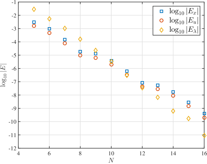
Refer to caption
Fig. 2: The base 10 logarithm of the error in the sup-norm as a function of the number of collocation points for Example 1.

8.2 Example 2

Next we consider the problem [33] given by

minimize 12​∫01[x2​(t)+u2​(t)]​𝑑t\displaystyle\quad\frac{1}{2}\int_{0}^{1}[x^{2}(t)+u^{2}(t)]\;dt
subject to x˙​(t)=u⁡(t),u⁡(t)≤1,x⁡(t)≤2​e1−efor all ​t∈[0,1],\displaystyle\quad\dot{x}(t)=u(t),\quad u(t)\leq 1,\quad x(t)\leq\frac{2\sqrt{e}}{1-e}\quad\mbox{for all }t\in[0,1],
x⁡(0)=5​e+34​(1−e).\displaystyle\quad x(0)=\frac{5e+3}{4(1-e)}.

The exact solution to this problem is

0≤t≤14:x∗​(t)=t−14+1+e1−e,u∗​(t)=1,14≤t≤34:x∗​(t)=et−141−e​(1+e32−2​t),u∗​(t)=et−141−e​(1−e32−2​t),34≤t≤1:x∗​(t)=2​e1−e,u∗​(t)=0.\begin{array}[]{lll}{0\leq t\leq\frac{1}{4}}:&x^{*}(t)=t-\frac{1}{4}+\frac{1+e}{1-e},&u^{*}(t)=1,\\[3.61371pt] {\frac{1}{4}\leq t\leq\frac{3}{4}}:&x^{*}(t)=\frac{e^{t-\frac{1}{4}}}{1-e}(1+e^{\frac{3}{2}-2t}),&u^{*}(t)=\frac{e^{t-\frac{1}{4}}}{1-e}(1-e^{\frac{3}{2}-2t}),\\[3.61371pt] {\frac{3}{4}\leq t\leq 1}:&x^{*}(t)=\frac{2\sqrt{e}}{1-e},&u^{*}(t)=0.\end{array}

The solution of this problem is smooth on the three intervals [0,0.25][0,0.25], [0.25,0.75][0.25,0.75], and [0.75,1.0][0.75,1.0], however, at the contact points where one of the constraints changes from active to inactive, there is a discontinuity in the derivative of the optimal control and a discontinuity in the second derivative of the optimal state. The goal with this test problem is to determine whether exponential convergence occurs for the h​php-scheme with a careful choice of the mesh, and whether a state constrained problem, which is not covered by the error analysis in this paper, possesses similar errors bounds to those for control constrained problems.

First, we solve the problem using K=1K=1, in which case convergence is achieved by increasing the degree NN of the polynomials. In Figure 3(a) we plot the logarithm of the error at the collocation points in the sup-norm versus the logarithm of the polynomial degree. Convergence occurs, but it is slow due to the discontinuity in the derivatives.

(a)Refer to caption (b)Refer to caption
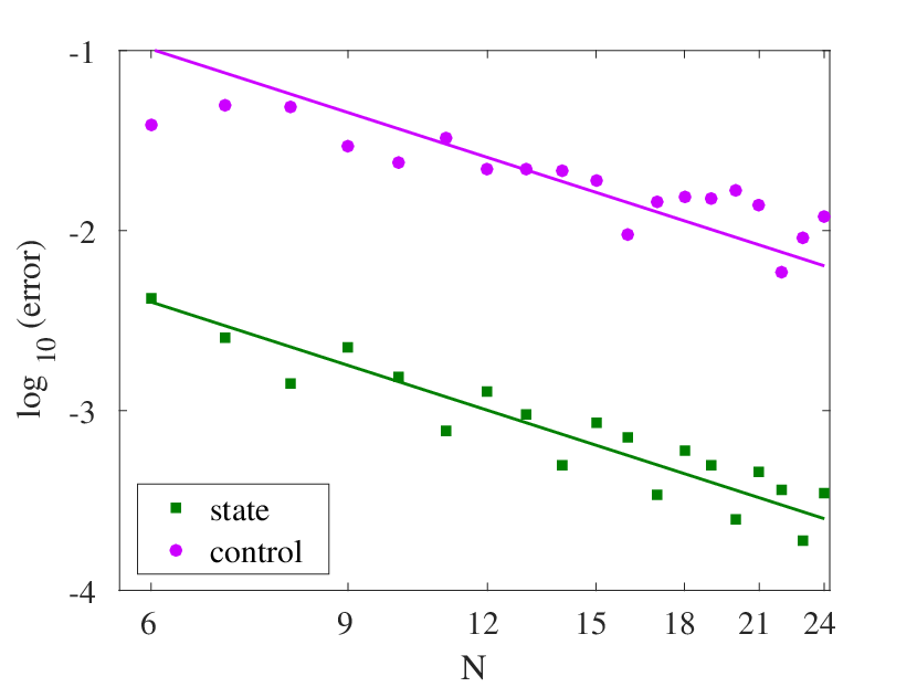
Fig. 3: The error in the solution to Example 2 as a function of the degree of the polynomials used in the h​php-approximation. In (a) the polynomials are defined on the interval [0,1][0,1]. In (b) there are three mesh intervals [0,0.25][0,0.25], [0.25,0.75][0.25,0.75], and [0.75,1.0][0.75,1.0], and different polynomials of the same degree are used on each mesh interval.

The lines in Figure 3(a) have slope −2-2; their vertical placement was chosen to achieve the best least squares fit to the markers (the measured error). Since the logarithm of the error is approximately fit by a line of slope −2-2, the error decays like c/N2c/N^{2}, which is faster than what might be expected from a bound like that given in Theorem 1 with regularity ℋ2.5−ϵ{\cal{H}}^{2.5-\epsilon} for any ϵ>0\epsilon>0.

Next, we divide the time interval [0,1] into three subintervals [0,0.25][0,0.25], [0.25,0.75][0.25,0.75], and [0.75,1.0][0.75,1.0], and use different polynomials of the same degree on each subinterval. By this careful choice of the mesh intervals, we obtain an exponential convergence rate in Figure 3(b). Comparing Figures 3(a) and 3(b), we see that a huge improvement in the error is possible when we have good estimates for the contact points where the constraints change between active and inactive. Note that 16-digit accuracy was obtained in Figure 3(b) by using MATLAB’s quadprog to solve the quadratic program associated with the h​php-discretization of Example 2.

In a very rough sense, the error bound given by Theorem 1 for a smooth problem has the general form c1​(c2/N)Nc_{1}(c_{2}/N)^{N}. The continuous curves plotted in Figure 3(b) were obtained by choosing c1c_{1} and c2c_{2} to achieve the least squares best fit to the markers (the measured error). For the state variable, (c1,c2)=(0.0016,0.1990)(c_{1},c_{2})=(0.0016,0.1990), while for the control (c1,c2)=(0.0950,0.2801)(c_{1},c_{2})=(0.0950,0.2801). Hence, it seems plausible that a state-constrained control problem may possess an error bound similar to that established in Theorem 1 for control constrained problems.

9 Conclusions

A convergence rate is derived for an h​php-orthogonal collocation method based on the Radau quadrature points applied to a control problem with convex control constraints. If the problem has a smooth local solution and a Hamiltonian which satisfies a strong convexity assumption, then the discrete approximation has a local minimizer in a neighborhood of the continuous solution. For the h​php-scheme, both the number of mesh intervals in the discretization and the degree of the polynomials on each mesh interval can be freely chosen. As the number of mesh intervals increases, convergence occurs at a polynomial rate relative to the mesh width. When there is control over the growth in derivatives, the convergence rate is exponentially fast relative to the polynomial degree. Convergence rates were investigated further using numerical examples. When the polynomial degree is fixed and the mesh width tends to zero, the observed convergence rate was faster than the rate associated with the error bound. For a problem with control and state constraints, exponentially fast convergence was observed when mesh points are located at the contact points where the constraints change between active and inactive. Based on the numerical results, it seems plausible that the convergence result established for control constrained problem could extend to problems with state constraints.

10 Appendix 1: Proof of (P1) and (P2)

We analyze (P1) and (P2) when τi\tau_{i}, 1≤i≤N1\leq i\leq N, are either the Radau quadrature points analyzed in this paper, or the Gauss quadrature points studied in [34].

Lemma 10.

For either the Gauss or Radau quadrature points, the rows of the matrix [𝐖1/2𝐃1:N]−1[{\bf{W}}^{1/2}{\bf{D}}_{1:N}]^{-1} have Euclidean length bounded by 2\sqrt{2}. For the Gauss quadrature points, ∥𝐃1:N−1∥∞≤2\|{\bf{D}}_{1:N}^{-1}\|_{\infty}\leq 2, and ∥𝐃1:N−1∥∞\|{\bf{D}}_{1:N}^{-1}\|_{\infty} approaches 22 as NN tends to infinity, while for the Radau quadrature points, ∥𝐃1:N−1∥∞=2\|{\bf{D}}_{1:N}^{-1}\|_{\infty}=2.

Proof.

Given 𝐩∈ℝN{\bf{p}}\in\mathbb{R}^{N}, let p∈𝒫Np\in{\cal{P}}_{N} denote the polynomial that satisfies p⁡(−1)=0p(-1)=0 and p⁡(τi)=pip(\tau_{i})=p_{i}, 1≤i≤N1\leq i\leq N. Let 𝐩˙∈ℝN\dot{{\bf{p}}}\in\mathbb{R}^{N} denote the vector with components p˙i=p˙​(τi)\dot{p}_{i}=\dot{p}(\tau_{i}), and let ℓj\ell_{j} be the Lagrange polynomial defined by

ℓj​(τ)=∏i=1i≠jNτ−τiτj−τi,1≤j≤N.\ell_{j}(\tau)=\prod^{N}_{\begin{subarray}{c}i=1\\ i\neq j\end{subarray}}\frac{\tau-\tau_{i}}{\tau_{j}-\tau_{i}},\quad 1\leq j\leq N.

The identity

p˙​(τ)=∑j=1Nℓj​(τ)​p˙j\dot{p}(\tau)=\sum_{j=1}^{N}\ell_{j}(\tau)\dot{p}_{j} (111)

holds since p˙∈𝒫N−1\dot{p}\in{\cal{P}}_{N-1} and the polynomials on each side of (111) are equal at the NN quadrature points. Integrate (111) to obtain

pi=∫−1τip˙​(τ)​𝑑τ=∑j=1N(∫−1τiℓj​(τ)​𝑑τ)​p˙j.p_{i}=\int_{-1}^{\tau_{i}}\dot{p}(\tau)\;d\tau=\sum_{j=1}^{N}\left(\int_{-1}^{\tau_{i}}\ell_{j}(\tau)\;d\tau\right)\dot{p}_{j}. (112)

Since 𝐃{\bf{D}} is a differentiation matrix and p⁡(−1)=0p(-1)=0, it follows that 𝐃1:N𝐩=𝐩˙{\bf{D}}_{1:N}{\bf{p}}=\dot{{\bf{p}}}. If the vector 𝐩˙=𝟎\dot{{\bf{p}}}={\bf{0}}, then the polynomial p˙=0\dot{p}=0 since p˙\dot{p} has degree N−1N-1 and vanishes at NN points. Since p⁡(−1)=0p(-1)=0, it follows that polynomial p=0p=0, which implies that the vector 𝐩=𝟎{\bf{p}}={\bf{0}}. Hence, 𝐃1:N{\bf{D}}_{1:N} is invertible, and 𝐩=𝐃−1​𝐩˙{\bf{p}}={\bf{D}}^{-1}\dot{{\bf{p}}}. Comparing the equality 𝐩=𝐃−1​𝐩˙{\bf{p}}={\bf{D}}^{-1}\dot{{\bf{p}}} to (112), we deduce that

(𝐃−1)i​j=∫−1τiℓj​(τ)​𝑑τ.({\bf{D}}^{-1})_{ij}=\int_{-1}^{\tau_{i}}\ell_{j}(\tau)\;d\tau. (113)

Choose any s∈[−1,1]s\in[-1,1] and define

dj​(s)=∫−1sℓj​(τ)​𝑑τandR⁡(s)=∑j=1Ndj​(s)2ωj.d_{j}(s)=\int_{-1}^{s}\ell_{j}(\tau)\;d\tau\quad\mbox{and}\quad R(s)=\sum_{j=1}^{N}\frac{d_{j}(s)^{2}}{\omega_{j}}.

Observe that (𝐃−1)i​j=dj​(τi)({\bf{D}}^{-1})_{ij}=d_{j}(\tau_{i}) and R⁡(τi)R(\tau_{i}) is the square of the Euclidean length of row ii in (𝐖1/2​𝐃)−1({\bf{W}}^{1/2}{\bf{D}})^{-1}. Let q∈𝒫N−1q\in{\cal{P}}_{N-1} be the polynomial defined by

q⁡(τ)=∑j=1Ndj​(s)​ℓj​(τ)ωj.q(\tau)=\sum_{j=1}^{N}\frac{d_{j}(s)\ell_{j}(\tau)}{\omega_{j}}.

Hence, by the triangle and Schwarz inequalities,

R⁡(s)=∫−1sq⁡(τ)​𝑑τ≤∫−11|q⁡(τ)|​𝑑τ≤2​(∫−11q​(τ)2​𝑑τ)1/2.R(s)=\int_{-1}^{s}q(\tau)\;d\tau\leq\int_{-1}^{1}|q(\tau)|\;d\tau\leq\sqrt{2}\left(\int_{-1}^{1}q(\tau)^{2}\;d\tau\right)^{1/2}. (114)

Since q2∈𝒫2​N−2q^{2}\in{\cal{P}}_{2N-2}, both Radau and Gauss quadrature are exact, and

∫−11q​(τ)2​𝑑τ=∑i=1Nωi​q​(τi)2,\int_{-1}^{1}q(\tau)^{2}\;d\tau=\sum_{i=1}^{N}\omega_{i}q(\tau_{i})^{2}, (115)

where the τj\tau_{j} are either the Radau or Gauss quadrature points and the ωj\omega_{j} are the associated weights. Since ℓj​(τi)=1\ell_{j}(\tau_{i})=1 for i=ji=j and ℓj​(τi)=0\ell_{j}(\tau_{i})=0 otherwise, it follows from the definition of qq that q⁡(τi)=di​(s)/ωiq(\tau_{i})=d_{i}(s)/\omega_{i}. This substitution in (115) yields

∫−11q​(τ)2​𝑑τ=∑i=1Ndi​(s)2ωj=R⁡(s).\int_{-1}^{1}q(\tau)^{2}\;d\tau=\sum_{i=1}^{N}\frac{d_{i}(s)^{2}}{\omega_{j}}=R(s). (116)

Equating the expressions (114) and (116) implies that

(∫−11q​(τ)2​𝑑τ)1/2≤2.\left(\int_{-1}^{1}q(\tau)^{2}\;d\tau\right)^{1/2}\leq\sqrt{2}.

By (116), R⁡(s)≤2R(s)\leq 2 for any s∈[−1,1]s\in[-1,1]. In particular, R⁡(τi)≤2R(\tau_{i})\leq 2 for 1≤i≤N1\leq i\leq N. Since R⁡(τi)R(\tau_{i}) is the square of the Euclidean length of row ii in (𝐖1/2​𝐃)−1({\bf{W}}^{1/2}{\bf{D}})^{-1}, the rows of (𝐖1/2​𝐃)−1({\bf{W}}^{1/2}{\bf{D}})^{-1} have Euclidean length bounded by 2\sqrt{2}. This result holds for both the Radau and Gauss quadrature points since since q2∈𝒫2​N−2q^{2}\in{\cal{P}}_{2N-2}, and both Radau and Gauss quadrature are exact for polynomials of this degree.

If 𝐫{\bf{r}} is a row of 𝐃1:N−1{\bf{D}}_{1:N}^{-1}, then by the Schwarz inequality and the fact that the quadrature weights sum to 2 and the rows of the matrix [𝐖1/2𝐃1:N]−1[{\bf{W}}^{1/2}{\bf{D}}_{1:N}]^{-1} have Euclidean length bounded by 2\sqrt{2}, we have

∑i=1N|ri|=∑i=1Nωi​(|ri|/ωi)≤(∑i=1Nωi)1/2​(∑i=1Nri2/ωi)1/2≤2.\sum_{i=1}^{N}|r_{i}|=\sum_{i=1}^{N}\sqrt{\omega_{i}}\left(|r_{i}|/\sqrt{\omega_{i}}\right)\leq\left(\sum_{i=1}^{N}\omega_{i}\right)^{1/2}\left(\sum_{i=1}^{N}r_{i}^{2}/\omega_{i}\right)^{1/2}\leq 2. (117)

Consequently, the absolute row sums for 𝐃1:N−1{\bf{D}}_{1:N}^{-1} are all bounded by 2, or equivalently, ∥𝐃1:N−1∥∞≤2\|{\bf{D}}_{1:N}^{-1}\|_{\infty}\leq 2. Given any polynomial p∈𝒫Np\in{\cal{P}}_{N} with p⁡(−1)=0p(-1)=0 and |p˙​(τi)|≤1|\dot{p}(\tau_{i})|\leq 1 for 1≤i≤N1\leq i\leq N, it is observed in Section 9 of [34] that ∥𝐃1:N−1∥∞≥\|{\bf{D}}_{1:N}^{-1}\|_{\infty}\geq max⁡{p⁡(τi):1≤i≤N}\max\{p(\tau_{i}):1\leq i\leq N\}. Take p⁡(τ)=1+τp(\tau)=1+\tau to deduce that ∥𝐃1:N−1∥∞≥1+τN\|{\bf{D}}_{1:N}^{-1}\|_{\infty}\geq 1+\tau_{N}. Hence, 1+τN≤∥𝐃1:N−1∥∞≤21+\tau_{N}\leq\|{\bf{D}}_{1:N}^{-1}\|_{\infty}\leq 2. Since τN=1\tau_{N}=1 for the Radau points, it follows that ∥𝐃1:N−1∥∞=2\|{\bf{D}}_{1:N}^{-1}\|_{\infty}=2. For the Gauss points, τN\tau_{N} approaches 1 as NN tends to infinity; consequently, ∥𝐃1:N−1∥∞\|{\bf{D}}_{1:N}^{-1}\|_{\infty} approaches 2 as NN tends to infinity for the Gauss points. ∎

11 Appendix 2: An analytic formula for (𝐃‡)−1({\bf D}^{\ddagger})^{-1}

Before stating property (P3) in the Introduction, we showed that 𝐃‡{\bf D}^{\ddagger} is an invertible matrix. In this section, we give an analytic formula for the inverse.

Proposition 11.

The inverse of 𝐃‡{\bf D}^{\ddagger} is given by

Di​j‡−1=ωN​Mj​(1)+∫1τiMj​(τ)​𝑑τ,1≤i<N,  1≤j<N,Di​N‡−1=−ωN,1≤i≤N,DN​j‡−1=ωN​Mj​(1),1≤j<N,\begin{array}[]{llll}D^{{\ddagger}\;-1}_{ij}&=&\omega_{N}M_{j}(1)+\displaystyle{\int_{1}^{\tau_{i}}M_{j}(\tau)d\tau,}&1\leq i<N,\;\;1\leq j<N,\\[3.61371pt] D^{{\ddagger}\;-1}_{iN}&=&-\omega_{N},&1\leq i\leq N,\\[3.61371pt] D^{{\ddagger}\;-1}_{Nj}&=&\omega_{N}M_{j}(1),&1\leq j<N,\end{array}

where MjM_{j}, 1≤j<N1\leq j<N, is the Lagrange interpolating basis relative to the point set τ1\tau_{1}, …\ldots, τN−1\tau_{N-1}. That is,

Mj(τ)=∏i=1i≠jN−1τ−τiτj−τi,j=1,…,N−1.M_{j}(\tau)=\displaystyle\prod_{\begin{subarray}{c}i=1\\ i\neq j\end{subarray}}^{N-1}\frac{\tau-\tau_{i}}{\tau_{j}-\tau_{i}},\quad j=1,\ldots,N-1.
Proof.

The relation (13) holds for any polynomial pp of degree at most N−1N-1. Let 𝐩˙∈ℝN\dot{{\bf{p}}}\in\mathbb{R}^{N} denote the vector with ii-th component p˙​(τi)\dot{p}(\tau_{i}). In vector form, the system of equations (13) can be expressed 𝐃‡​𝐩={\bf D}^{\ddagger}{\bf p}= 𝐩˙−𝐞N​p​(1)/ωN\dot{\bf p}-{\bf{e}}_{N}p(1)/\omega_{N}. Multiply by 𝐃‡−1{\bf{D}}^{{\ddagger}\;-1} and exploit the identity 𝐃‡−1​𝐞N=−ωN​𝟏{\bf{D}}^{{\ddagger}\;-1}{\bf{e}}_{N}=-\omega_{N}{\bf{1}} of (82) to obtain

𝐃‡−1​𝐩˙=𝐩−𝟏​p​(1).{\bf D}^{{\ddagger}\;-1}\dot{{\bf{p}}}={\bf{p}}-{\bf{1}}p(1). (118)

Since p˙\dot{p} is a polynomial of degree at most N−2N-2, we can only specify the derivative of pp at N−1N-1 distinct points. Given any jj satisfying 1≤j<N1\leq j<N, let us insert in (118) a polynomial p∈𝒫N−1p\in{\cal{P}}_{N-1} satisfying

p˙​(τj)=1andp˙​(τi)=0​ for all ​i<N,i≠j.\dot{p}(\tau_{j})=1\quad\mbox{and}\quad\dot{p}(\tau_{i})=0\mbox{ for all }i<N,\;\;i\neq j.

A specific polynomial with this property is

p⁡(τ)=∫1τMj​(τ)​𝑑τ.p(\tau)=\int_{1}^{\tau}M_{j}(\tau)d\tau. (119)

Since pN=p⁡(1)=0p_{N}=p(1)=0, the last component of the right side of (118) vanishes to give the relation DN​j‡−1+DN​N‡−1​p˙​(1)=0D_{Nj}^{{\ddagger}\;-1}+D_{NN}^{{\ddagger}\;-1}\dot{p}(1)=0. In (82) we showed that all the elements in the last column of 𝐃‡−1{\bf{D}}^{{\ddagger}\;-1} are equal to −ωN-\omega_{N}, and by (119), p˙​(1)=Mj​(1)\dot{p}(1)=M_{j}(1). Hence, we obtain the relation

DN​j‡−1=−DN​N‡−1​p˙​(1)=ωN​p˙​(1)=ωN​Mj​(1),  1≤j<N.D_{Nj}^{{\ddagger}\;-1}=-D_{NN}^{{\ddagger}\;-1}\dot{p}(1)=\omega_{N}\dot{p}(1)=\omega_{N}M_{j}(1),\;\;1\leq j<N. (120)

Finally, let us consider Di​j‡−1D_{ij}^{{\ddagger}\;-1} for i<Ni<N and j<Nj<N. We combine the ii-th component of (118) for i<Ni<N with (119) to obtain

(𝐃‡−1​𝐩˙)i=∫1τiMj​(τ)​𝑑τ.({\bf D}^{{\ddagger}\;-1}\dot{{\bf{p}}})_{i}=\int_{1}^{\tau_{i}}M_{j}(\tau)d\tau. (121)

Recall that all components of 𝐩˙\dot{{\bf{p}}} vanish except for the jj-th, which is 1, and the NN-th, which is Mj​(1)M_{j}(1) by (119). Hence, (121) and the fact that the elements in the last column of 𝐃‡−1{\bf{D}}^{{\ddagger}\;-1} are all −ωN-\omega_{N} yield

Di​j‡−1=∫1τiMj​(τ)​𝑑τ−Di​N‡−1​Mj​(1)=ωN​Mj​(1)+∫1τiMj​(τ)​𝑑τD_{ij}^{{\ddagger}\;-1}=\int_{1}^{\tau_{i}}M_{j}(\tau)d\tau-D_{iN}^{{\ddagger}\;-1}M_{j}(1)=\omega_{N}M_{j}(1)+\int_{1}^{\tau_{i}}M_{j}(\tau)d\tau

This completes the proof. ∎

Tables 1 and 2 show ‖𝐃‡−1‖∞\|{\bf{D}}^{{\ddagger}\;-1}\|_{\infty} and the maximum Euclidean norm of the rows of 𝐃‡−1𝐖−1/2{\bf{D}}^{{\ddagger}\;-1}{\bf{W}}^{-1/2} for an increasing sequence of dimensions. The norms in Table 1 approach 2 as NN grows, consistent with (P3), while the norms in Table 2 approach 2\sqrt{2}, consistent with (P4).

NN 25 50 75 100 125 150
norm 1.995376 1.998844 1.999486 1.999711 1.999815 1.999871
NN 175 200 225 250 275 300
norm 1.999906 1.999928 1.999943 1.999954 1.999962 1.999968
Table 1: ‖𝐃‡−1‖∞\|{\bf D}^{{\ddagger}\;-1}\|_{\infty}
NN 25 50 75 100 125 150
norm 1.412209 1.413691 1.413982 1.414083 1.414130 1.414156
NN 175 200 225 250 275 300
norm 1.414171 1.414181 1.414188 1.414193 1.414196 1.414199
Table 2: Maximum Euclidean norm for the rows of [𝐖1/2​𝐃‡]−1[{\bf{W}}^{1/2}{\bf D}^{\ddagger}]^{-1}

References

  • [1] I. Babuška and M. Suri, The h-p version of the finite element method with quasiuniform meshes, RAIRO, Modélisation Mathématique et Analyse Numérique, 21 (1987), pp. 199–238.
  • [2]  , The p- and h-p version of the finite element method, an overview, Comput. Methods Appl. Mech. Engrg., 80 (1990), pp. 5–26.
  • [3]  , The p and h-p version of the finite element method, basic principles and properties, SIAM Rev., 36 (1994), pp. 578–632.
  • [4] D. A. Benson, G. T. Huntington, T. P. Thorvaldsen, and A. V. Rao, Direct trajectory optimization and costate estimation via an orthogonal collocation method, J. Guid. Control Dyn., 29 (2006), pp. 1435–1440.
  • [5] C. Bernardi and Y. Maday, Polynomial interpolation results in Sobolev spaces, J. Comput. Appl. Math., 43 (1992), pp. 53–82.
  • [6] J. T. Betts, Sparse optimization suite, Applied Mathematical Analysis, LLC, Issaquah, WA, 2013.
  • [7] L. T. Biegler and V. M. Zavala, Large-scale nonlinear programming using IPOPT: An integrating framework for enterprise-wide optimization, Comput. Chem. Eng., 33 (2008), pp. 575–582.
  • [8] J. F. Bonnans and J. Laurent-Varin, Computation of order conditions for symplectic partitioned Runge-Kutta schemes with application to optimal control, Numer. Math., 103 (2006), pp. 1–10.
  • [9] C. Canuto, M. Hussaini, A. Quarteroni, and T. Zang, Spectral methods, Fundamentals in single domains, Springer, 2006.
  • [10] C. L. Darby, W. W. Hager, and A. V. Rao, Direct trajectory optimization using a variable low-order adaptive pseudospectral method, J. Spacecr. Rockets, 48 (2011), pp. 433–445.
  • [11]  , An hp-adaptive pseudospectral method for solving optimal control problems, Optim. Control Appl. Meth., 32 (2011), pp. 476–502.
  • [12] A. Dontchev, W. W. Hager, A. Poore, and B. Yang, Optimality, stability, and convergence in nonlinear control, Applied Math. and Optim., 31 (1995), pp. 297–326.
  • [13] A. L. Dontchev and W. W. Hager, Lipschitzian stability in nonlinear control and optimization, SIAM J. Control Optim., 31 (1993), pp. 569–603.
  • [14]  , A new approach to Lipschitz continuity in state constrained optimal control, Systems and Control Letters, 35 (1998), pp. 137–143.
  • [15]  , The Euler approximation in state constrained optimal control, Math. Comp., 70 (2001), pp. 173–203.
  • [16] A. L. Dontchev, W. W. Hager, and V. M. Veliov, Second-order Runge-Kutta approximations in constrained optimal control, SIAM J. Numer. Anal., 38 (2000), pp. 202–226.
  • [17] G. Elnagar, M. Kazemi, and M. Razzaghi, The pseudospectral Legendre method for discretizing optimal control problems, IEEE Trans. Automat. Control, 40 (1995), pp. 1793–1796.
  • [18] G. N. Elnagar and M. A. Kazemi, Pseudospectral Chebyshev optimal control of constrained nonlinear dynamical systems, Comput. Optim. Appl., 11 (1998), pp. 195–217.
  • [19] J. Elschner, The h-p-version of spline approximation methods for Melin convolution equations, J. Integral Equations Appl., 5 (1993), pp. 47–73.
  • [20] F. Fahroo and I. M. Ross, Costate estimation by a Legendre pseudospectral method, J. Guid. Control Dyn., 24 (2001), pp. 270–277.
  • [21]  , Direct trajectory optimization by a Chebyshev pseudospectral method, J. Guid. Control Dyn., 25 (2002), pp. 160–166.
  • [22] D. Garg, M. A. Patterson, C. L. Darby, C. Françolin, G. T. Huntington, W. W. Hager, and A. V. Rao, Direct trajectory optimization and costate estimation of finite-horizon and infinite-horizon optimal control problems using a Radau pseudospectral method, Comput. Optim. Appl., 49 (2011), pp. 335–358.
  • [23] D. Garg, M. A. Patterson, W. W. Hager, A. V. Rao, D. A. Benson, and G. T. Huntington, A unified framework for the numerical solution of optimal control problems using pseudospectral methods, Automatica, 46 (2010), pp. 1843–1851.
  • [24] Q. Gong, I. M. Ross, W. Kang, and F. Fahroo, Connections between the covector mapping theorem and convergence of pseudospectral methods for optimal control, Comput. Optim. Appl., 41 (2008), pp. 307–335.
  • [25] W. Gui and I. Babuška, The h, p and h-p versions of the finite element method in 1 dimension. Part I. The error analysis of the p-version, Numer. Math., 49 (1986), pp. 577–612.
  • [26]  , The h, p and h-p versions of the finite element method in 1 dimension. Part II. The error analysis of the h-and h-p versions, Numer. Math., 49 (1986), pp. 613–657.
  • [27]  , The h, p and h-p versions of the finite element method in 1 dimension. Part III. The adaptive h-p version, Numer. Math., 49 (1986), pp. 659–683.
  • [28] W. W. Hager, Multiplier methods for nonlinear optimal control, SIAM J. Numer. Anal., 27 (1990), pp. 1061–1080.
  • [29]  , Runge-Kutta methods in optimal control and the transformed adjoint system, Numer. Math., 87 (2000), pp. 247–282.
  • [30]  , Numerical analysis in optimal control, in International Series of Numerical Mathematics, K.-H. Hoffmann, I. Lasiecka, G. Leugering, J. Sprekels, and F. Tröltzsch, eds., vol. 139, Basel/Switzerland, 2001, Birkhauser Verlag, pp. 83–93.
  • [31] W. W. Hager, H. Hou, and A. V. Rao, Convergence rate for a Radau collocation method applied to unconstrained optimal control, (2015, arXiv: 1508.03783).
  • [32]  , Convergence rate for a Gauss collocation method applied to unconstrained optimal control, J. Optim. Theory Appl., 169 (2016), pp. 801–824.
  • [33] W. W. Hager and G. Ianculescu, Dual approximations in optimal control, SIAM J. Control Optim., 22 (1984), pp. 423–465.
  • [34] W. W. Hager, J. Liu, S. Mohapatra, A. V. Rao, and X.-S. Wang, Convergence rate for a Gauss collocation method applied to constrained optimal control, SIAM J. Control Optim., 56 (2018), pp. 1386–1411.
  • [35] R. A. Horn and C. R. Johnson, Matrix Analysis, Cambridge University Press, Cambridge, 2013.
  • [36] W. Kang, The rate of convergence for a pseudospectral optimal control method, in Proceeding of the 47th IEEE Conference on Decision and Control, IEEE, 2008, pp. 521–527.
  • [37]  , Rate of convergence for the Legendre pseudospectral optimal control of feedback linearizable systems, J. Control Theory Appl., 8 (2010), pp. 391–405.
  • [38] F. Liu, W. W. Hager, and A. V. Rao, Adaptive mesh refinement method for optimal control using nonsmoothness detection and mesh size reduction, J. Franklin Inst., 352 (2015), pp. 4081–4106.
  • [39] J. Nocedal and S. J. Wright, Numerical Optimization, Springer, New York, 2nd ed., 2006.
  • [40] M. A. Patterson, W. W. Hager, and A. V. Rao, A p​hph mesh refinement method for optimal control, Optim. Control Appl. Meth., 36 (2015), pp. 398–421.
  • [41] M. A. Patterson and A. V. Rao, GPOPS-II: A MATLAB software for solving multi-phase optimal control problems using hp-adaptive Gaussian quadrature collocation methods and sparse non-linear programming, ACM Trans. Math. Software, 41 (2014), pp. 1–37.
  • [42] M. A. Patterson and A. V. Rao, 𝔾​ℙ​𝕆​ℙ​𝕊−𝕀​𝕀\mathbb{GPOPS-II}, a MATLAB software for solving multiple-phase optimal control problems using h​php-adaptive Gaussian quadrature collocation methods and sparse nonlinear programming, ACM Transactions on Mathematical Software, 41 (2015), pp. 1–37.
  • [43] J. Shen, T. Tang, and L.-L. Wang, Spectral Methods, Springer, Berlin, 2011.
  • [44] G. Szegő, Orthogonal Polynomials, American Mathematical Society, Providence, RI, 1939.
  • [45] P. Williams, Jacobi pseudospectral method for solving optimal control problems, J. Guid. Control Dyn., 27 (2004), pp. 293–297.