Unitarity and microscopic acausality in a nonlocal theory

In the absence of higher-derivative modifications, we work with a theory of $N$ real scalar fields with the Lagrangian density

$${\cal L}=\frac{1}{2}\partial_{\mu}\phi^{a}\partial^{\mu}\phi^{a}-\frac{1}{2}m^{2}\,\phi^{a}\phi^{a}-\frac{1}{8}\lambda_{0}(\phi^{a}\phi^{a})^{2}\,\,\,.$$

(4)

This theory has an O($N$) global symmetry, with the index $a$ running from $1$ to $N$. The theory has a sensible $N\rightarrow\infty$ limit, i.e., there are no Feynman diagrams that grow as positive powers of $N$, if the coupling $\lambda_{0}$ scales as $1/N$. (For a pedagogical discussion, see Ref. [22].) It is convenient to redefine the coupling $\lambda_{0}\equiv\lambda/N$, so that the $N$ dependence of a given amplitude is explicit. Following Ref. [19], the theory in Eq. (4) is equivalent to

$${\cal L}=\frac{1}{2}\partial_{\mu}\phi^{a}\partial^{\mu}\phi^{a}-\frac{1}{2}m^{2}\,\phi^{a}\phi^{a}+\frac{N}{2\lambda}\sigma^{2}-\frac{1}{2}\sigma\phi^{a}\phi^{a}\,\,\,,$$

(5)

where $\sigma$ is an auxiliary field; this can be verified by substitution of the auxiliary field’s equation of motion into Eq. (5). The advantage of working with the auxiliary field formulation is that it makes counting of powers of $N$ transparent, since each $\sigma$ propagator scales as $1/N$. For example, the self-energy function for the $\sigma$ field, $\Sigma_{0}(p^{2})$, receives it’s leading order contribution from a $\phi^{a}$ loop, and scales as $N$. Following the sign conventions of Ref. [19], the full $\sigma$ propagator is given by

$$\tilde{D}(p^{2})=\frac{i}{1/\lambda_{0}}+\frac{i}{1/\lambda_{0}}\left(i\Sigma_{0}\right)\frac{i}{1/\lambda_{0}}+\frac{i}{1/\lambda_{0}}\left(i\Sigma_{0}\right)\frac{i}{1/\lambda_{0}}\left(i\Sigma_{0}\right)\frac{i}{1/\lambda_{0}}+\cdots\,\,\,,$$

(6)

which can be re-summed to

$$\tilde{D}(p^{2})=\frac{\lambda}{N}\frac{i}{1+\lambda\,\Sigma(p^{2})}\,\,\,,$$

(7)

where $\Sigma_{0}(p^{2})\equiv N\,\Sigma(p^{2})$, so that the $N$-scaling of Eq. (7) is explicit. All corrections to $\Sigma(p^{2})$ that are higher than one-loop are suppressed by additional factors of $1/N$, by virtue of the additional $\sigma$ propagators. Hence, if one is interested in only the leading-order behavior of $\Sigma(p^{2})$, one only needs to compute a one-loop diagram¹¹ 1 At leading order there is also a one-loop $\sigma$ tadpole diagram, but it can be eliminated by a shift in the auxiliary field and a redefinition of the $\phi^{a}$ mass [22]..

At leading order in $1/N$, two-into-two scattering in the auxiliary field formulation corresponds to the $s$-, $t$- and $u$- channel exchanges of the auxiliary field, with the dressed propagator given by Eq. (7). All other loop corrections to the scattering amplitude involve additional $\sigma$ propagators and are sub-leading in the $1/N$ expansion. It follows that the scattering amplitude is given by

$${\cal M}(ab\rightarrow cd)=-\frac{\lambda}{N}\left[\frac{\delta_{ab}\delta_{cd}}{1+\lambda\Sigma(s)}+\frac{\delta_{ac}\delta_{bd}}{1+\lambda\Sigma(t)}+\frac{\delta_{ad}\delta_{bc}}{1+\lambda\Sigma(u)}\right]\,\,\,,$$

(8)

where $s$, $t$ and $u$ are the usual Mandelstam invariants. As reviewed in Ref. [19], Eq. (8) can be used to demonstrate the unitarity of the theory at leading order in $1/N$ and at all orders in perturbation theory.

Our present interest is how this calculation is altered when there is a nonlocal modification to Eq. (4), of either the form

$${\cal L}=-\frac{1}{2}\phi^{a}\,\hat{F}(\Box)^{-1}(\Box+m^{2})\,\phi^{a}-\frac{1}{8}\lambda_{0}(\phi^{a}\phi^{a})^{2}\,\,\,,$$

(9)

or

$${\cal L}=-\frac{1}{2}\phi^{a}\,(\Box+m^{2})\,\phi^{a}-\frac{1}{8}\lambda_{0}\left[(\hat{F}^{1/2}\phi^{a})(\hat{F}^{1/2}\phi^{a})\right]^{2}\,\,\,.$$

(10)

Here $\hat{F}$ is the differential operator defined in Eq. (3), with $\eta>0$ and $n$ and even positive integer, and $\hat{F}^{1/2}\equiv\exp(-\frac{1}{2}\eta\!\stackrel{{\scriptstyle}}{{\Box}}^{n})$. We choose $n$ even so that the factors of $\hat{F}$ lead to improved convergence of loop integrals in momentum space, regardless of whether we assume a Euclidean or Minkowski metric. We compare each possibility in the following subsection, for the simplest choice of $n=2$, which we assume henceforth. Eqs. (9) and (10) are related by a nonlocal field redefinition and give the same results for scattering amplitudes. Working with Eq. (10), the factors of $\hat{F}^{1/2}$ acting on internal lines reproduce the momentum dependence of the propagator that one obtains from Eq. (9); the factors of $\hat{F}^{1/2}$ acting on external lines each give a factor of $\exp(-\eta\,m^{4}/2)$, matching the wave function renormalization factors in the scattering amplitudes obtained from Eq. (9). For definiteness, we will examine the case where $a=b\neq c=d$ so that only the $s$-channel amplitudes is relevant. Then the scattering amplitude takes the form

$${\cal M}=-\frac{\lambda}{N}\frac{e^{-2\eta\,m^{4}}}{1+\lambda\,\Sigma(s)}\,\delta_{ab}\delta_{cd}\,\,\,,$$

(11)

where the constant exponential factor is due to the higher-derivative operator acting on the external lines, and where $\Sigma(s)$ now includes the effects of $\hat{F}$ on the $\phi^{a}$ propagator.

We show in this section that the theory defined in Minkowski space by Eq. (10) violates unitarity. The self-energy function $\Sigma(p^{2})$ is given by

$$\Sigma(p^{2})=-\frac{i}{2}\int\frac{d^{4}k}{(2\pi)^{4}}\frac{\exp\{-\eta\,(k+p/2)^{4}\}\exp\{-\eta\,(k-p/2)^{4}\}}{[(k-p/2)^{2}-m^{2}+i\epsilon][(k+p/2)^{2}-m^{2}+i\epsilon]}\,\,\,.$$

(12)

Unitarity implies the operator relation $i(T^{\dagger}-T)=T^{\dagger}T$, where the $T$-matrix is related to the $S$-matrix by $S=1+iT$. One can derive a condition on scattering amplitudes by taking matrix elements of both sides of this expression and including an appropriate insertion of a complete set of intermediate states. Working at leading order in the $1/N$ expansion, this procedure was carried out in the O(N) model in Ref. [19], and the derivation is not altered by the presence of the additional momentum space suppression factors in the numerator of Eq. (12). One finds [19]

	$\displaystyle 2\mbox{ Im}$	$\displaystyle\!\!{\cal M}$	$\displaystyle\!\!(k_{1},a;k_{2},b\rightarrow k_{1}^{\prime},c;k_{2}^{\prime},d)=\sum_{e,f}I_{e,f}\int\frac{d^{3}q_{1}}{(2\pi)^{3}}\frac{d^{3}q_{2}}{(2\pi)^{3}}\frac{1}{2E_{1}}\frac{1}{2E_{2}}(2\pi)^{4}\delta^{(4)}(q_{1}+q_{2}-p)$		(13)
			$\displaystyle{\cal M}(k_{1},a;k_{2},b\rightarrow q_{1},e;q_{2},f)\,{\cal M}^{*}(k_{1}^{\prime},c;k_{2}^{\prime},d\rightarrow q_{1},e;q_{2},f)\,\,\,,$

where the identical particle factor $I_{e,f}=1/2$ if $e=f$ and $1$ otherwise. The left-hand-side of this expression follows immediately from Eq. (11):

$$LHS=\frac{\lambda^{2}}{N}\left[2\,e^{-2\,\eta\,m^{4}}\mbox{ Im }\Sigma(s)\right]\frac{1}{|1+\lambda\,\Sigma(s)|^{2}}\,\delta_{ab}\delta_{cd}\,\,\,.$$

(14)

The right-hand-side of Eq. (13) includes only two-particle intermediate states, which provide the leading contribution in the large $N$ limit. After substitution of Eq. (11), the necessary integral evaluation is identical to that of the two-body Lorentz-invariant phase space factor. The result is

$$RHS=\frac{\lambda^{2}}{N}\left[\frac{1}{16\pi}e^{-4\,\eta\,m^{4}}\sqrt{1-\frac{4m^{2}}{s}}\,\right]\frac{1}{|1+\lambda\,\Sigma(s)|^{2}}\,\delta_{ab}\delta_{cd}\,\,\,.$$

(15)

When $\eta=0$, the quantities in brackets in Eqs. (14) and (15) coincide, as can be seen either from an elementary one-loop calculation [19], or by examining the $\eta\rightarrow 0$ limit of the numerical calculation that we are about to describe. When $\eta\neq 0$, these quantities differ. After exploring the source of the discrepancy, we show how it is avoided by defining the theory as an analytic continuation of correlation functions defined in Euclidean space.

It is easiest to see that Eqs. (14) and (15) do not agree when $\eta\neq 0$ by showing that $\mbox{Im }\Sigma(p^{2})$ no longer has a functional form proportional to $\sqrt{1-4\,m^{2}/s}$. To confirm this claim most quickly, we simply evaluate the imaginary part of Eq. (12) numerically, working in the center-of-mass frame, where $\vec{p}=0$; we perform the $k^{0}$ integral exactly along the real axis with $\epsilon$ finite and evaluate the limit as $\epsilon\rightarrow 0$. Note that the imaginary part of the loop integral is finite, even when $\eta$ is vanishing. It is convenient to write Eq. (12) in the following form:

$$\mbox{Im }\Sigma=-\frac{1}{4\pi^{3}}\int_{0}^{\infty}dk\int_{0}^{\infty}dk^{0}\left\{k^{2}g(k^{0},k)\frac{f_{+}(k^{0},k)f_{-}(k^{0},k)-\epsilon^{2}}{\left[f_{+}(k^{0},k)^{2}+\epsilon^{2}\right]\left[f_{-}(k^{0},k)^{2}+\epsilon^{2}\right]}\right\}\,\,\,,$$

(16)

where $k\equiv|\vec{k}|$,

$$f_{\pm}(k^{0},k)\equiv(k^{0}\pm p^{0}/2)^{2}-k^{2}-m^{2}\,\,\,,$$

(17)

and

$$g(k^{0},k)\equiv\exp\{-\eta[(k^{0}+p^{0}/2)^{2}-k^{2}]^{2}-\eta[(k^{0}-p^{0}/2)^{2}-k^{2}]^{2}\}\,\,\,.$$

(18)

The integration can be performed using symbolic mathematics code (we used MAPLE [23]), provided care is taken in dealing with the points on the real $k^{0}$ axis that would be singularities in the $\epsilon\rightarrow 0$ limit. For $\epsilon$ small but non-zero, the growth of the integrand around these points are taken into account by singularity handling routines in MAPLE that are invoked automatically by breaking up the region of $k^{0}$ integration into intervals that are terminated at these points. We then have no difficulty obtaining numerically convergent results. In Fig. 1, we show the result for $\mbox{Im }\Sigma$ as a function of the center-of-mass energy, working in units where $m=1$, for $\eta=0$ and an example where $\eta\neq 0$. The line with long dashes shows the expectation for $\mbox{Im }\Sigma$ following from the analytic result of the one-loop calculation in the $\eta=0$ case,

$$\mbox{Im }\Sigma(s)=\frac{1}{32\pi}\sqrt{1-\frac{4m^{2}}{s}}\theta(s-4m^{2})\,\,\,,$$

(19)

where $\theta$ is the Heaviside step function. This agrees with the numerical result for $\eta=0$, given by the open circular points in Fig. 1. However, the results are not proportional to the same functional form in $s$ for the case where $\eta\neq 0$. One would not suspect that the disagreement is the result of a numerical artifact, since the extra exponential factor in the integrand in the case where $\eta\neq 0$ is smooth and serves primarily to truncate the domain of integration.

To further verify this result, let us now do the calculation in a different way. Imagine we evaluate the $k^{0}$ integral in $\Sigma$ by closing a semi-circular contour in the lower-half complex plane. In ordinary, local quantum field theories, the integral along the semi-circular contour would vanish as the radius of the contour is taken to infinity. In the present theory, this is not the case; the numerator of the loop integral becomes $\exp[-2\,\eta\,(k^{0})^{4}]$ far from the origin, which blows up in directions where $\mbox{Re }(k^{0})^{4}<0$. Hence, let us decompose

$$\Sigma=\Sigma_{p}-I_{C}\,\,\,\,\mbox{ and }\,\,\,\,2\,\mbox{Im}\,\Sigma=2\,\mbox{Im}\,\Sigma_{p}-2\,\mbox{Im}\,I_{C}\,\,\,,$$

(20)

where $\Sigma_{p}$ is $-2\pi i$ times the residues of the poles contained within the contour and $I_{C}$ is the clockwise integral along the semi-circular portion. Since

$$\Sigma_{p}(p^{0})=\frac{1}{2}\int\frac{d^{3}k}{(2\pi)^{3}}\frac{1}{2E_{\vec{k}}\,p^{0}}\left[\frac{N(k^{0}=E_{\vec{k}}-p^{0}/2)}{2E_{\vec{k}}-p^{0}}-\frac{N(k^{0}=E_{\vec{k}}+p^{0}/2)}{2E_{\vec{k}}+p^{0}}\right]\,\,\,,$$

(21)

where $N$ represents the numerator of the integrand of Eq. (12) and $E^{2}_{\vec{k}}\equiv|\vec{k}|^{2}+m^{2}$, it is clear for $0<p^{0}<2m$ on the real axis that $\Sigma_{p}(p^{0})=\Sigma_{p}(p^{0*})^{*}$. Since $\Sigma_{p}$ is an analytic function of $p^{0}$ off the real axis, this can be analytically continued, from which it follows that

$$\mbox{Disc}\,\Sigma_{p}=2\,i\,\mbox{Im}\,\Sigma_{p}(p^{0}+i\epsilon)\,\,\,,$$

(22)

where the discontinuity is about a cut on the real $p^{0}$ axis,

$$\mbox{Disc}\,\Sigma_{p}=\lim_{\epsilon\rightarrow 0}\left[\Sigma_{p}(p^{0}+i\epsilon)-\Sigma_{p}(p^{0}-i\epsilon)\right]\,\,\,.$$

(23)

We may express

	$\displaystyle\Sigma_{p}(p^{0}+i\epsilon)$	$\displaystyle=$	$\displaystyle\frac{1}{8\pi^{2}}\int dE_{\vec{k}}\frac{|\vec{k}|}{p^{0}+i\epsilon}$		(24)
			$\displaystyle\times\left[\frac{N(k^{0}=E_{\vec{k}}-p^{0}/2-i\epsilon/2)}{2E_{\vec{k}}-p^{0}-i\epsilon}-\frac{N(k^{0}=E_{\vec{k}}+p^{0}/2+i\epsilon/2)}{2E_{\vec{k}}+p^{0}+i\epsilon}\right]\,\,\,.$

There can be poles in the $E_{\vec{k}}$ integration that blow up at most as $1/\epsilon$; hence, we only need expand what remains to order $\epsilon$. Defining $N^{\prime}\equiv\partial N/\partial k^{0}$, we find

$$\begin{split}\mbox{Disc}\,\Sigma_{p}&=-\frac{1}{8\pi^{2}}\lim_{\epsilon\rightarrow 0}\int dE_{\vec{k}}\frac{|\vec{k}|}{p^{0}}\\ &\left\{N(k^{0}=k^{0}_{-})\left[\frac{1}{p^{0}-2E_{\vec{k}}+i\epsilon}-\frac{1}{p^{0}-2E_{\vec{k}}-i\epsilon}\right]\right.\\ &+N(k^{0}=k^{0}_{+})\left[\frac{1}{p^{0}+2E_{\vec{k}}+i\epsilon}-\frac{1}{p^{0}+2E_{\vec{k}}-i\epsilon}\right]\\ &+\left[\frac{-i}{2}N^{\prime}(k^{0}=k^{0}_{-})-\frac{i}{p^{0}}N(k^{0}=k^{0}_{-})\right]\left[\frac{\epsilon}{p^{0}-2E_{\vec{k}}+i\epsilon}+\frac{\epsilon}{p^{0}-2E_{\vec{k}}-i\epsilon}\right]\\ &\left.+\left[\frac{i}{2}N^{\prime}(k^{0}=k^{0}_{+})-\frac{i}{p^{0}}N(k^{0}=k^{0}_{+})\right]\left[\frac{\epsilon}{p^{0}+2E_{\vec{k}}+i\epsilon}+\frac{\epsilon}{p^{0}+2E_{\vec{k}}-i\epsilon}\right]\right\}\end{split}$$

(25)

where $k^{0}_{\pm}=E_{\vec{k}}\pm p^{0}/2$. We can now take the $\epsilon\rightarrow 0$ limits of the quantities in square brackets, using

$$\lim_{\epsilon\rightarrow 0}\left[\frac{1}{y+i\epsilon}-\frac{1}{y-i\epsilon}\right]=-2\pi i\,\delta(y)\,\,\,\mbox{ and }\,\,\,\lim_{\epsilon\rightarrow 0}\left[\frac{\epsilon}{y+i\epsilon}+\frac{\epsilon}{y-i\epsilon}\right]=2\pi y\,\delta(y)\,\,\,.$$

(26)

We see that the third and fourth terms in the curly braces are proportional to $(p^{0}\pm 2E_{\vec{k}})\delta(p^{0}\pm 2E_{\vec{k}})$, so that they vanish after integration. Since $p^{0}>0$, the surviving term is given by

$$\mbox{Disc}\,\Sigma_{p}=i\frac{1}{4\pi}\int dE_{\vec{k}}\,\frac{|\vec{k}|}{p^{0}}\,\delta(p^{0}-2E_{\vec{k}})\,N(k^{0}=E_{\vec{k}}-p^{0}/2)$$

(27)

It is straightforward to confirm that the same result is obtained by making the conventional Cutkosky replacements in the original integral for $\Sigma_{p}$

$$\frac{1}{(k\pm p/2)^{2}-m^{2}+i\epsilon}\rightarrow-2\pi i\,\delta([k\pm p/2]^{2}-m^{2})$$

(28)

so that

$$i\,\mbox{Disc}\,\Sigma_{p}=\frac{1}{2}\int\frac{d^{4}k}{(2\pi)^{4}}N(k)(-2\pi i)^{2}\delta([k+p/2]^{2}-m^{2}))\delta([k-p/2]^{2}-m^{2})\,\,\,.$$

(29)

Changing variables, introducing an additional integral, and writing out the numerator factor $N$, this is equivalent to

$$\begin{split}i\,\mbox{Disc}\,\Sigma_{p}&=\\ -\frac{1}{2}&\int\frac{d^{4}q_{1}}{(2\pi)^{4}}\frac{d^{4}q_{2}}{(2\pi)^{4}}\,e^{(-\eta\,q_{1}^{4}-\eta\,q_{2}^{4})}\,(2\pi)\delta(q_{1}^{2}-m^{2})\,(2\pi)\delta(q_{2}^{2}-m^{2})\\ &(2\pi)^{4}\delta^{(4)}(q_{1}+q_{2}-p)\,\,\,,\end{split}$$

(30)

which integrates to

$$i\,\mbox{Disc}\,\Sigma_{p}=-\frac{1}{16\pi}e^{-2\,\eta\,m^{4}}\sqrt{1-\frac{4m^{2}}{s}}\,\,\,.$$

(31)

From Eqs. (20) and (22), it follows that we can write the quantity in square brackets from the left-hand-side of our unitarity relation, Eq. (14), as

$$\left[2\,e^{-2\,\eta\,m^{4}}\mbox{ Im }\Sigma(s)\right]=\frac{1}{16\pi}e^{-4\,\eta\,m^{4}}\sqrt{1-\frac{4m^{2}}{s}}-2\,e^{-2\,\eta\,m^{4}}\,\mbox{Im}\,I_{C}\,\,\,.$$

(32)

The first term agrees with the desired form of the quantity in square brackets in Eq. (15); it follows that the violation of unitarity stems entirely from the non-vanishing of the integral $I_{C}$ along the semi-circular contour.

We can verify that Eq. (32) is correct by evaluating the imaginary part of $I_{C}$ and comparing the result for $\mbox{Im}\,\Sigma$ with what we obtained previously in Fig. 1. Notice that if we were to push all the poles on the real $k^{0}$ axis to the upper half-plane, then $I_{C}$ would be given by the negative of the integral along the real axis. Hence, we may identify

$$I_{C}=\frac{i}{2}\int\frac{d^{4}k}{(2\pi)^{4}}\frac{N(k)}{\left[(k^{0}-p^{0}/2-i\epsilon)^{2}-E_{\vec{k}}^{2}\right]\left[(k^{0}+p^{0}/2-i\epsilon)^{2}-E_{\vec{k}}^{2}\right]}\,\,\,.$$

(33)

The point is that Eq. (33) can be evaluated numerically in exactly the same way as the integral in Eq. (12) that we described earlier. The result for $\mbox{Im}\,\Sigma$ computed from Eq. (32) using the numerical evaluation of Eq. (33) is indicated by the solid points shown in Fig. 1: they are in complete agreement with our previous direct evaluation of $\mbox{Im}\,\Sigma$ in the case where $\eta\neq 0$.

To understand this result, it is useful to consider how the calculation might have proceeded had we started by evaluating the discontinuity of Eq. (12) directly using Cutkosky’s formula [24]. It is straightforward to check that the discontinuity computed in this way would reconcile Eq. (14) and Eq. (15) only if $\mbox{Disc}\,\Sigma=2\,i\,\mbox{Im}\,\Sigma$. However, this relation is not justified in the present case since $\Sigma$ cannot be shown to satisfy the Schwartz reflection principle $\Sigma(p^{0})=\Sigma(p^{0*})^{*}$ when $\eta\neq 0$. The reflection principle requires that there be a segment along the real $p^{0}$ axis over which $\Sigma$ is purely real; in the case where $\eta\neq 0$ it is not possible to prove that such a region exists and our numerical results shown in Fig. 1 strongly suggest that the opposite is true. In the Appendix, we show in more detail how the violation of the Scwartz reflection principle can be directly related to the non-vanishing of contour integrals, like $I_{C}$, at large radius in the complex plane.

Another starting point [8] for attempts to demonstrate unitarity is the Largest Time Equation (LTE) [25]. We simply note here that this approach cannot be consistently applied to the present problem. As discussed by Anselmi [26], derivation of the LTE requires two assumptions: (1) the vertices of the theory are localized time and (2) the propagator in position space is of the form $\theta(x^{0})g_{+}(x)+\theta(-x^{0})g_{-}(x)$, where $\theta$ is the step function. If nonlocality appears in the vertices of the theory, then assumption (1) is violated. If a field redefinition is used to move the nonlocality to the propagators, then assumption (2) is violated due to the appearance of additional terms in the propagator that are proportional to derivatives of $\delta(x^{0})$. (The explicit form of the propagator can be found in Ref. [16].) The subsequent derivation of the LTE described in Ref. [26] fails. Hence, we say nothing further about this approach.

We have discussed in the previous subsection how unitarity is violated if we attempt to formulate the theory of interest directly in Minkowski space. If correlation functions are defined in Euclidean space and analytically continued in the external momenta to Minkowski space, unitarity is preserved. This might be expected since the theory quantized via a Euclidean functional integral automatically satisfies reflection positivity. The way that the calculation of the previous section is modified is as follows: The Euclidean version of $\Sigma$ corresponds to Eq. (12) with the $k^{0}$ integration taken along the imaginary axis, and with Euclidean external momentum $p^{0}=ip^{0}_{E}$. In other words, the starting point is the path that one would obtain with a Wick rotation if it were justified in a Minkowski-space formulation of the theory. Now, close the contour with a semi-circle in the right half plane, so that

$$2\,\mbox{Im}\,\Sigma=2\,\mbox{Im}\,\Sigma_{p}-2\,\mbox{Im}\,I_{C}^{\prime}\,\,\,,$$

(34)

where $I_{C}^{\prime}$ is the integral over the semi-circular path, and $\Sigma_{p}$ again is determined by the residues of the poles contained within the closed contour. While $\mbox{Im}\,I_{C}$ in our previous calculation was non-vanishing, we now show that $\mbox{Im}\,I_{C}^{\prime}=0$. Let us write $I_{C}^{\prime}=-i\int dk^{0}X(k^{0})$, where $X(k^{0})$ is given by Eq. (12) with $\epsilon$ set to zero and $k^{0}$ placed on the desired semi-circle, $k^{0}=\rho\exp(i\theta)$ for $-\pi/2\leq\theta\leq\pi/2$. In the center-of-mass frame where $\vec{p}=0$, it is straightforward to check that $X(k^{0})$ is also a function of ${p^{0}}^{2}={-{p^{0}_{E}}^{2}}$, which is real; it follows immediately that $X(k^{0})^{*}=X(k^{0*})$. Since $dk^{0}=ik^{0}d\theta$,

$$2\,i\,\mbox{Im}\,I_{C}^{\prime}=I_{C}^{\prime}-I_{C}^{\prime*}=\lim_{\rho\rightarrow\infty}\int_{-\pi/2}^{\pi/2}d\theta\left[k^{0}X(k^{0})-k^{0*}X(k^{0*})\right]\,\,\,,$$

(35)

which vanishes; this can be seen by changing variables $\theta\rightarrow-\theta$, and noting that $k^{0}(-\theta)=k^{0*}$, indicating that the $d\theta$ integral is equal to its negative. The surviving term in Eq. (34) is the same function of $p^{0}$ that reconciled the left- and right-hand-sides of our unitarity relation in the previous section. By Lorentz invariance, the result holds in any other reference frame in which the scattering process is measured. Hence, we have verified that the large $N$ scattering amplitudes of interest in the present context are unitary provided that the theory is defined as in Ref. [5], via the analytic continuation to Minkowski-space external momentum of correlation functions defined in a Euclidean field theory. We will assume that correlation functions are computed in this way in the discussion that follows.

The Feynman-propagator $D_{F}(x-y)$ is identified with the two-point correlation function $\langle 0|T\phi(x)\phi(y)|0\rangle$. If we strictly assume that $x^{0}>y^{0}$, then we may write the commutator

$$\langle 0|[\phi(x),\phi(y)]|0\rangle=D_{F}(x-y)-D_{F}(x-y)^{*}\,\,\,\,\,\,\,\,\,\,(x^{0}>y^{0})\,\,\,.$$

(36)

Working with the form of the theory in which the higher-derivative operator appears in the quadratic terms for $\phi$, it follows immediately that²² 2 Since we work here with the lowest-order propagator, our prescription of starting with a Euclidean correlation function and continuing to Minkowski space in the external momentum simply gives us the usual momentum-space propagator. All subsequent Fourier transforms are, of course, in Minkowski space.

$$D_{F}(x-y)=\int\frac{d^{4}k}{(2\pi)^{4}}\frac{i\,e^{-\eta\,k^{4}}}{k^{2}-m^{2}+i\epsilon}e^{-ik\cdot(x-y)}\,\,\,.$$

(37)

Because the factor of $e^{-\eta\,k^{4}}$ blows up in certain directions in the complex $k^{0}$ plane, as indicated earlier, the usual procedure of closing the integration contour in the lower half plane is not useful; instead we directly evaluate the $k^{0}$ integral along the real axis, deviating by small semi-circles below and above the poles at $k^{0}=-E_{\vec{k}}$ and $+E_{\vec{k}}$, respectively. Hence, we may write $D_{F}(x-y)=I_{2C}+I_{PV}$, where $I_{2C}$ is the result from the semi-circle integrations while $I_{PV}$ is the remaining principal value integral. The latter can be reduced to a one-dimensional integral in the case $m=0$, which we can numerically evaluate. We find

$$I_{2C}=\frac{1}{4\pi^{2}|\vec{r}|}\int_{0}^{\infty}dk\sin(k\,|\vec{r}|)\cos(k\,r^{0})\,\,\,,$$

(38)

where we define $r=x-y$ and $k=|\vec{k}|$. The remaining principal value integral is identical to one considered in the computation of the retarded propagator for this theory in Ref. [6], and is given by

$$I_{PV}=\frac{-i}{\pi^{3}}\frac{\partial}{\partial\rho}\left[\mbox{sign}(\rho)\int_{0}^{\infty}\frac{dy}{y}\exp(-\eta y^{4}/\rho^{2})\left[K_{0}(y)+\frac{\pi}{2}Y_{0}(y)\right]\right]\,\,\,.$$

(39)

where $\rho={r^{0}}^{2}-|\vec{r}|^{2}$. Restricting to the case where $r^{0}<|\vec{r}|$, it follows from Eqs. (36) and (39) that

$$\langle 0|[\phi(x),\phi(y)]|0\rangle=\frac{4\,i\,\eta}{\pi^{3}\rho^{3}}\int_{0}^{\infty}dy\,y^{3}\exp(-\eta\,y^{4}/\rho^{2})\left[K_{0}(y)+\frac{\pi}{2}Y_{0}(y)\right]\,,\,\,\,\,\,\,\,(0<r^{0}<|\vec{r}|)\,\,\,,$$

(40)

where $K_{0}$ and $Y_{0}$ are Bessel functions. Eq. (40) is nonvanishing, as is shown in Fig. 2. We do not consider the case $m\neq 0$, since the necessary two-dimensional numerical integration is much more tedious but no more illuminating.

One might wonder how this calculation of the commutator relates to a similar calculation in the formulation of the theory where the nonlocality appears only in the interaction terms, Eq. (10). The unstated assumption is that the theory presented in this form results from a field redefinition starting with the theory in which only the quadratic terms are modified, Eq. (9). With nonlocal interactions arising in this way, operators that correspond to observables are built out of the “smeared” fields, $\hat{F}^{1/2}\phi(x)$, and it is the commutator of these objects that is the physically relevant quantity to evaluate at space-like separation. This gives precisely the same integral to evaluate as in Eq. (37), with a different origin for the momentum dependence in the numerator.

The question we now wish to address is how acausality manifests itself in the time-dependence of scattering processes. We allow ourselves to stray from the O($N$) model in this subsection to consider theories of a single real scalar field with the same modification of their quadratic terms as Eq. (9), but with different interaction terms. This will allow us to illustrate the effects of interest most clearly; the generalization to the O($N$) model that we previously considered will be clear by analogy. We consider two examples, following the general approach of Ref. [19]:

Particle Production by a Source. Consider a local theory of a real scalar field which includes a coupling to a classical source,

$${\cal L}_{int}=\phi(x)j(x)\,\,\,,$$

(41)

where ${\cal L}_{int}$ is the interaction Lagrangian. We wish to study $\langle\psi_{out}|\Omega\rangle$, the amplitude for the source to create an outgoing wave-packet state from the vacuum, where

$$|\psi_{out}\rangle=\int d^{4}x^{\prime}g(x^{\prime}-y^{\prime})\,\phi(x^{\prime})\,|\Omega\rangle\,\,\,.$$

(42)

Here we follow the convections of Ref. [19] where primed coordinates correspond to “out” states. The function $g(x^{\prime})$ is chosen so that the outgoing wave packet is localized about the space-time point $y^{\prime}$ at some time long after the source is turned off, and its four-momentum is localized about $p^{\prime}$. By the choice of this function, we can determine the position of the wave-packet at any earlier time when the source is turned on. For a source localized within a small region about the spacetime origin, we first show that the amplitude vanishes if the wave-packet’s trajectory extrapolates back to the origin at a time substantially earlier than $t=0$, as one would expect for a causal process. We then consider how this conclusion changes given the chosen nonlocal modification of this theory.

The amplitude $\langle\psi_{out}|\Omega\rangle$ may be written

	$\displaystyle\langle\psi_{out}|\Omega\rangle$	$\displaystyle=$	$\displaystyle\int d^{4}x^{\prime}g^{*}(x^{\prime}-y^{\prime})\langle\Omega|\phi(x^{\prime})|\Omega\rangle$		(43)
		$\displaystyle=$	$\displaystyle i\int d^{4}y\,j(y)\int\frac{d^{4}p}{(2\pi)^{4}}\frac{i}{p^{2}-m^{2}+i\epsilon}\,\tilde{g}(p)^{*}\,e^{-ip\cdot(y^{\prime}-y)}$
		$\displaystyle\equiv$	$\displaystyle i\int d^{4}y\,j(y)\,I(y^{\prime}-y)\,\,\,,$

where $\tilde{g}(p)$ is the Fourier transform $\tilde{g}(p)=\int\!d^{4}x\,g(x)\,e^{ip\cdot x}$. As we discussed earlier, all momentum-space correlation functions are defined via analytic continuation from a Euclidean theory; all subsequent calculations, including Fourier transforms, are then performed in Minkowski space. The integral $I(y^{\prime}-y)$ can be re-expressed using a Schwinger parameter,

$$I(\Delta y)=\frac{1}{\hbar}\int_{0}^{\infty}ds\int\frac{d^{4}p}{(2\pi)^{4}}\,e^{is(p^{2}-m^{2}+i\epsilon)/\hbar}\,\tilde{g}(p)^{*}\,e^{-ip\cdot\Delta y/\hbar}\,\,\,,$$

(44)

where $\Delta y\equiv y^{\prime}-y$, and we have temporarily restored the $\hbar$ dependence. As in Ref. [19], if the relevant distance scales (in this case $\Delta y$) are large compared to all characteristic inverse masses and inverse momenta, then we are justified in using the stationary phase approximation, since this limit is equivalent to taking $\hbar\rightarrow 0$ in Eq. (44). Evaluating the $d^{4}p$ integral in this way (and resuming our convention that $\hbar=1$) yields

$$I(\Delta y)=\frac{i}{16\pi^{2}}\int_{0}^{\infty}ds\,\frac{1}{s^{2}}\,\tilde{g}(\frac{\Delta y}{2s})^{*}\,e^{-i[\Delta y^{2}/(4s)+sm^{2}]}\,\,\,.$$

(45)

By evaluating the $ds$ integral in the same way one finds

$$I(\Delta y)=\frac{\sqrt{i}}{4\sqrt{2}\pi^{3/2}}\frac{m^{1/2}}{(\Delta y^{2})^{3/4}}\tilde{g}(m\frac{\Delta y}{\sqrt{\Delta y^{2}}})^{*}e^{-im\sqrt{\Delta y^{2}}}\,\,\,,$$

(46)

leading finally to

$$\langle\psi_{out}|\Omega\rangle=\frac{1}{2}\left(\frac{i}{2\pi}\right)^{3/2}\int d^{4}y\,\frac{m^{1/2}}{[(y^{\prime}-y)^{2}]^{3/4}}\,j(y)\,\tilde{g}\!\left(m\frac{y^{\prime}-y}{\sqrt{(y^{\prime}-y)^{2}}}\right)^{*}e^{-im\sqrt{(y^{\prime}-y)^{2}}}\,\,\,.$$

(47)

By construction, the function $\tilde{g}$ only has support in the region where

$$m\frac{(y^{\prime}-y)}{\sqrt{(y^{\prime}-y)^{2}}}\approx p^{\prime}\,\,\,,$$

(48)

which limits the possible values of $y$ that contribute to the integral. Let us assume a $\tilde{g}$ in which $\vec{y}\approx 0$ for some $y^{0}\ll 0$. If $j(y)$ is strongly localized about the spacetime origin, for example a delta function source $j(y)\propto\delta^{(4)}(y)$, the integral in Eq. (47) vanishes. The “production vertex” for the outgoing wave packet, which is identified spatially with the origin, cannot occur before the time at which the source excites the system.

The conclusion is different if we introduce a nonlocal coupling to the source following our earlier prescription

$${\cal L}_{int}=[\hat{F}^{1/2}\phi(x)]j(x)\,\,\,.$$

(49)

This case is simple to understand since we can integrate by parts, and recover a theory of the original form, but with a “smeared” source,

$$j(y)_{s}=\hat{F}^{1/2}j(y)=\int d^{4}x\,\epsilon(y-x)\,j(x)\,\,\,\,\,\mbox{ where }\,\,\,\,\,\epsilon(y-x)=\int\frac{d^{4}k}{(2\pi)^{4}}e^{-\eta\,k^{4}/2}\,e^{ik\cdot(y-x)}\,\,\,.$$

(50)

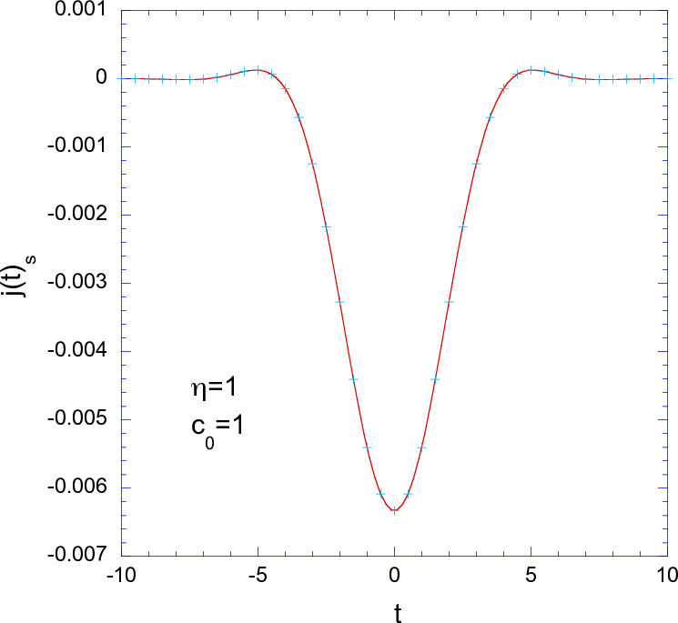
Assuming the example where $j(y)=c_{0}\,\delta^{(4)}(y)$, where $c_{0}$ is a coupling, consider the time-dependence of $j(y)_{s}$ near the spatial origin

	$\displaystyle j(y^{0},\vec{y}=0)_{s}$	$\displaystyle=$	$\displaystyle\frac{c_{0}}{2\pi^{3}}\int_{0}^{\infty}dk^{0}\int_{0}^{\infty}dk\,k^{2}\exp[-\eta\,({k^{0}}^{2}-k^{2})^{2}/2]\cos(k^{0}y^{0})$		(51)
		$\displaystyle=$	$\displaystyle\frac{c_{0}}{8\sqrt{2}\pi^{3}}\int_{0}^{\infty}dk^{0}\,{k^{0}}^{3}e^{-\eta\,k0^{4}/4}\cos[k^{0}y^{0}]\left[K_{1/4}({k^{0}}^{4})-K_{3/4}({k^{0}}^{4})\right]\,\,\,,$

where $K_{i}$ is a Bessel function of the second kind, of order $i$. Unlike the original $j(x)$, this function is no longer localized in time at $t=0$. The second line of Eq. (51) can be evaluated numerically and the results are shown in Fig. 3. This result implies that there is a common region with $y^{0}\ll 0$ and $\vec{y}\approx\vec{0}$ where the functions $j$ and $\tilde{g}$ in Eq. (47) both have support; the overlap $\langle\psi_{out}|\Omega\rangle$ is therefore generally nonvanishing. One concludes that there is a non-vanishing probability that the wave packet appears to emerge from the position of a spatially localized source at a time before the system has been excited by the source.

Two-into-two scattering. The previous example is perhaps the simplest illustration of how the smearing of interaction positions can lead to the apparent acausal ordering of scattering events. In the more phenomenologically relevant case of two-into-two scattering, similar results can be obtained. We use the term “apparent” since the spacetime positions of the production and the subsequent decay of a resonance, for example, are inferred from the wave packet positions and momenta long before and after the interaction has occurred. Nothing meaningful can be said about the system directly at intermediate times, since no measurements are made during this period. We now consider how the wave-packet analysis of two-into-two scattering discussed in the context of Lee-Wick theories in Ref. [19] is modified in the present context.

We consider the same free theory of a real scalar field $\phi$, and introduce couplings to two additional real scalar fields $\psi$ and $\chi$, that would otherwise have no higher-derivative couplings. In this case we assume

$${\cal L}_{int}=\frac{1}{2}g_{\chi}(\hat{F}^{1/2}\phi)\chi^{2}+\frac{1}{2}g_{\psi}(\hat{F}^{1/2}\phi)\psi^{2}\,\,\,,$$

(52)

Again, this is consistent with the assumption that we start with a theory in which the higher-derivative operators appear in the $\phi$ quadratic terms only, and that these terms have been subsequently put in canonical form by a field redefinition. We do not consider doing the same for the $\psi$ and $\chi$ fields to simplify the analysis; there is no reason to expect that this choice will affect our conclusions qualitatively. We consider the scattering process $\chi\chi\rightarrow\psi\psi$. Setting the problem up in the way that we have is convenient since the nonlocality affects the propagator but not the external lines, which allows us to immediately carry over most of the wave-packet analysis of Ref. [19] without modification. Let us briefly recapitulate the key steps in this approach.

We assume incoming and outgoing wavepacket states given by

	$\displaystyle|\psi_{in}\rangle$	$\displaystyle=\int d^{4}x_{1}d^{4}x_{2}f_{1}(x_{1}-y_{1})f_{2}(x_{2}-y_{2})\phi(x_{1})\phi(x_{2})|\Omega\rangle\,\,\ ,$		(53)
	$\displaystyle|\psi_{out}\rangle$	$\displaystyle=\int d^{4}x^{\prime}_{1}d^{4}x^{\prime}_{2}g_{1}(x^{\prime}_{1}-y^{\prime}_{1})g_{2}(x^{\prime}_{2}-y^{\prime}_{2})\phi(x^{\prime}_{1})\phi(x^{\prime}_{2})|\Omega\rangle\,\,\,,$		(54)

where the functions $f_{i}$ and $g_{i}$ define the wavepackets. These are chosen so that in the process of interest, we can specify well-defined production and decay vertices for the resonance, in this case associated with the field $\phi$, exchanged in the $s$-channel. To be more explicit, the functions $f_{i}$ are chosen so that the initial wavepackets are localized about the space-like separated points $y_{1}$ and $y_{2}$, respectively, and have momenta peaked at $p_{1}=m_{\chi}v_{1}$ and $p_{2}=m_{\chi}v_{2}$. A production vertex can be defined at point $z_{0}$, where

$$\frac{z_{0}-y_{1}}{\tau_{1}}=v_{1}\,\,\,\,\,\mbox{ and }\,\,\,\,\,\frac{z_{0}-y_{2}}{\tau_{2}}=v_{2}\,\,\,,$$

(55)

with $\tau_{i}^{2}\equiv(z_{0}-y_{i})^{2}$. Similarly, the functions $g_{i}$ are chosen so that the final wavepackets are localized about the space-like separated points $y^{\prime}_{1}$ and $y^{\prime}_{2}$, respectively, and have momenta peaked at $p^{\prime}_{1}=m_{\psi}v^{\prime}_{1}$ and $p^{\prime}_{2}=m_{\psi}v^{\prime}_{2}$. A decay vertex can be defined at point $z_{0}^{\prime}$ where

$$\frac{y^{\prime}_{1}-z^{\prime}_{0}}{\tau^{\prime}_{1}}=v^{\prime}_{1}\,\,\,\,\,\mbox{ and }\,\,\,\,\,\frac{y^{\prime}_{2}-z^{\prime}_{0}}{\tau^{\prime}_{2}}=v^{\prime}_{2}\,\,\,,$$

(56)

with ${\tau^{\prime}}_{i}^{2}\equiv(y^{\prime}_{i}-z^{\prime}_{0})^{2}$. Defining $w^{\mu}\equiv{z^{\prime}}_{0}^{\mu}-z_{0}^{\mu}$, the authors of Ref. [19] determined how the amplitude $\langle\psi_{out}|\psi_{in}\rangle$ depends on $w^{0}$ and showed in Lee-Wick theories that the amplitude is non-vanishing for an acausal ordering of the vertices. The key intermediate steps are these: the amplitude of interest can be written in the form

$$\langle\psi_{out}|\psi_{in}\rangle=\int\frac{d^{4}q}{(2\pi)^{4}}\tilde{F}(q)\tilde{G}(q)\Gamma^{(4)}_{s}(q^{2})\,\,\,,$$

(57)

where $\Gamma^{(4)}_{s}(q^{2})$ is the momentum-space four-point function for the $s$-channel process of interest, with propagators truncated from the external lines, and

	$\displaystyle\tilde{F}(q)$	$\displaystyle=\int d^{4}z\,e^{iz\cdot q}\,I_{1}(z)I_{2}(z)\,\,\,\,\,\mbox{ with}$		(58)
	$\displaystyle I_{i}(z)$	$\displaystyle=\int\frac{d^{4}k_{i}}{(2\pi)^{4}}\,e^{ik_{i}\cdot(y_{i}-z)}\tilde{f}_{i}(k_{i})\,\frac{i}{k_{i}^{2}-m^{2}+i\epsilon}\,\,\,,$		(59)

where $\tilde{f}_{i}(k)$ are the Fourier transforms of the incoming wave packet functions. We do not display the analogous expressions for $G(q)$, corresponding to the outgoing wave packet states. In the same limit described in our earlier example involving a classical source, the momentum and $z$ integrals in Eq. (59) can be evaluated in the stationary phase approximation, leading to a result of the form

$$\langle\psi_{out}|\psi_{in}\rangle\simeq\int\frac{d^{4}q}{(2\pi)^{4}}\,e^{-iq\cdot(z_{0}^{\prime}-z_{0})}\,\hat{F}(q)\,\hat{G}(q)\,\Gamma^{(4)}_{s}(q^{2})\,\,\,,$$

(60)

where the functions $\hat{F}$ and $\hat{G}$ have localized support at $q\approx p_{1}+p_{2}$ and $q\approx p^{\prime}_{1}+p^{\prime}_{2}$, respectively. We study the nonlocal theory of interest using Eq. (60) as the starting point. Hence, from Eq. (52) it follows that

$$\langle\psi_{out}|\psi_{in}\rangle=\int\frac{d^{4}q}{(2\pi)^{4}}\,e^{-iq\cdot w}\left[\frac{-i\,g_{\chi}\,g_{\psi}\,e^{-\eta\,q^{4}}}{q^{2}-m_{\phi}^{2}+i\,m\,\Gamma}\right]\,\hat{F}(q)\,\hat{G}(q)\,\,\,,$$

(61)

where $\Gamma$ is the $\phi$ decay width. Defining the Fourier transform

$$\epsilon^{\prime}(x)=\int\frac{d^{4}q}{(2\pi)^{4}}\,e^{-\eta\,q^{4}}\,e^{iq\cdot x}\,\,\,\,,$$

(62)

the amplitude can be written as

$$\langle\psi_{out}|\psi_{in}\rangle=\int d^{4}x\,\epsilon(x-w)I(x)\,\,\,,$$

(63)

where

$$I(x)=\frac{\sqrt{i}g_{\phi}g_{\chi}}{{8\pi^{3/2}}}\frac{m_{\phi}^{1/2}}{(\sqrt{x^{2}})^{3/2}}e^{-i\,m_{\phi}\sqrt{x^{2}}}\,e^{-\Gamma\sqrt{x^{2}}/2}\hat{F}(m_{\phi}\frac{x}{\sqrt{x^{2}}})\,\hat{G}(m_{\phi}\frac{x}{\sqrt{x^{2}}})\,\,\,.$$

(64)

As in the case of the “ordinary resonance” discussed in Ref. [19], as well as in our previous example, $I(x)$ is derived by exponentiating the propagator denominator using a Schwinger parameter and then integrating using the stationary phase approximation. Note that we cannot apply this approximation to Eq. (61) directly since we require that the nonlocal length scale $\eta^{1/4}$ to be comparable to the vertex separation; one cannot then assume that the real exponential prefactor is a slowly varying function of the momentum relative to the complex phase factor. Eq. (64) coincides with the ordinary resonance result when $\eta=0$, in which case $\epsilon^{\prime}$ becomes a four-dimensional delta function. In that limit, the argument of Ref. [19] is the following: in the center-of-mass frame, $\hat{F}$ and $\hat{G}$ only have support where $x^{0}=w^{0}>0$ and $\vec{x}=\vec{w}\approx 0$. Hence the amplitude is only nonvanishing for the causal ordering of the production and decay vertices. (In the Lee-Wick case, the result is the opposite.) Making the same assumptions here, one concludes only that $x^{0}$ must be greater than zero; the amplitude may be nonvanishing, for example, when $w^{0}<0$ and $\vec{w}=0$, since $\epsilon^{\prime}(x-w)$ is no longer a delta function. This can be verified by noting that the function $\epsilon^{\prime}$ differs from the function $\epsilon$ that we have previously studied by the replacement $\eta\rightarrow 2\eta$. Since the $x$ integral is dominated by the region where $\vec{x}\approx 0$, we can evaluate $\epsilon(x-w)$ for the choice $\vec{x}=\vec{w}=0$, where $\vec{w}=0$ corresponds to the case in which the production and decay vertices are spatially coincident. Since $\epsilon^{\prime}$ is non-vanishing for $x^{0}>0$ and $w^{0}<0$ we conclude that $\epsilon^{\prime}$, $\hat{F}$ and $\hat{G}$ have common regions of support, so that Eq. (63) is generally non-vanishing. Hence, there is a non-vanishing amplitude for an acausal ordering of the production and decay vertices. The effect emerges in a very different way than in the Lee-Wick theories. In that case, a crucial sign flip in the propagator of the Lee-Wick resonance leads to a change from $w^{0}$ to $-w^{0}$ in comparison to the ordinary resonance case. The sign flip affects the sign of the width appearing in one of the exponential factors in the amplitude, leading to the interpretation that the exponential decay is happening as the Lee-Wick resonance propagates backward in time from the decay to production vertex. Here, however, the form of $I(x)$ corresponds to propagation forward in time over the time-like interval $x$. The nonlocality in the theory leads to a spatial smearing of the interaction points so that one no longer identifies $x$ with the physical spacetime separation of the extrapolated decay and production vertices.

References

- [1] T. D. Lee and G. C. Wick, “Negative Metric and the Unitarity of the S Matrix,” Nucl. Phys. B 9, 209 (1969); “Finite Theory of Quantum Electrodynamics,” Phys. Rev. D 2, 1033 (1970).
- [2] B. Grinstein, D. O’Connell and M. B. Wise, “The Lee-Wick standard model,” Phys. Rev. D 77, 025012 (2008).
- [3] R. E. Cutkosky, P. V. Landshoff, D. I. Olive and J. C. Polkinghorne, “A non-analytic S matrix,” Nucl. Phys. B 12, 281 (1969).
- [4] For example, see N. Barnaby and N. Kamran, “Dynamics with infinitely many derivatives: The Initial value problem,” JHEP 0802, 008 (2008). For a nonperturbative treatment of similar theories, see G. Calcagni, M. Montobbio and G. Nardelli, “Localization of nonlocal theories,” Phys. Lett. B 662, 285 (2008).
- [5] T. Biswas and N. Okada, “Towards LHC physics with nonlocal Standard Model,” Nucl. Phys. B 898, 113 (2015).
- [6] A. Pais and G. E. Uhlenbeck, “On Field theories with nonlocalized action,” Phys. Rev. 79, 145 (1950).
- [7] N. Barnaby and J. M. Cline, “Large Nongaussianity from Nonlocal Inflation,” JCAP 0707, 017 (2007).
- [8] E. T. Tomboulis, “Superrenormalizable gauge and gravitational theories,” hep-th/9702146.
- [9] L. Modesto, “Super-renormalizable Quantum Gravity,” Phys. Rev. D 86, 044005 (2012).
- [10] T. Biswas, E. Gerwick, T. Koivisto and A. Mazumdar, “Towards singularity and ghost free theories of gravity,” Phys. Rev. Lett. 108, 031101 (2012).
- [11] T. Biswas, A. Conroy, A. S. Koshelev and A. Mazumdar, “Generalized ghost-free quadratic curvature gravity,” Class. Quant. Grav. 31, 015022 (2014) Erratum: [Class. Quant. Grav. 31, 159501 (2014)] .
- [12] L. Modesto, “Multidimensional finite quantum gravity,” arXiv:1402.6795 [hep-th].
- [13] L. Modesto and L. Rachwal, “Super-renormalizable and finite gravitational theories,” Nucl. Phys. B 889, 228 (2014).
- [14] L. Modesto, M. Piva and L. Rachwal, “Finite quantum gauge theories,” arXiv:1506.06227 [hep-th].
- [15] A. Addazi, Int. J. Mod. Phys. A 31, no. 04n05, 1650009 (2016).
- [16] E. T. Tomboulis, “Nonlocal and quasilocal field theories,” Phys. Rev. D 92, no. 12, 125037 (2015).
- [17] E. Witten, “Noncommutative Geometry and String Field Theory,” Nucl. Phys. B 268, 253 (1986); V. A. Kostelecky and S. Samuel, “On a Nonperturbative Vacuum for the Open Bosonic String,” Nucl. Phys. B 336, 263 (1990); V. A. Kostelecky and S. Samuel, “The Static Tachyon Potential in the Open Bosonic String Theory,” Phys. Lett. B 207, 169 (1988).
- [18] P. G. O. Freund and M. Olson, “Nonarchimedean Strings,” Phys. Lett. B 199, 186 (1987); P. G. O. Freund and E. Witten, “Adelic String Amplitudes,” Phys. Lett. B 199, 191 (1987); L. Brekke, P. G. O. Freund, M. Olson and E. Witten, “Nonarchimedean String Dynamics,” Nucl. Phys. B 302, 365 (1988).
- [19] B. Grinstein, D. O’Connell and M. B. Wise, “Causality as an emergent macroscopic phenomenon: The Lee-Wick O(N) model,” Phys. Rev. D 79, 105019 (2009).
- [20] S. Coleman, in Subnuclear Phenomena, Proceedings of the 7th International School of Subnuclear Physics, edited by A. Zichichi (Academic Press, New York, 1970) p. 282.
- [21] V. A. Alebastrov and G. V. Efimov, “A proof of the unitarity of S-matrix in a nonlocal quantum field theory,” Commun. Math. Phys. 31, no. 1, 1 (1973).
- [22] S. Coleman, “Aspects of Symmetry,” Cambridge University Press (1985) p. 351.
- [23] Maple 17. Maplesoft, a division of Waterloo Maple Inc., Waterloo, Ontario.
- [24] R. E. Cutkosky, “Singularities and discontinuities of Feynman amplitudes,” J. Math. Phys. 1, 429 (1960). doi:10.1063/1.1703676
- [25] M. J. G. Veltman, “Unitarity and causality in a renormalizable field theory with unstable particles,” Physica 29, 186 (1963). doi:10.1016/S0031-8914(63)80277-3
- [26] D. Anselmi, “Aspects of perturbative unitarity,” Phys. Rev. D 94, 025028 (2016) doi:10.1103/PhysRevD.94.025028 [arXiv:1606.06348 [hep-th]].