Algorithm on rainbow connection for maximal outerplanar graphsThanks: The project supported partially by CNNSF (No.11401181)and the first author is supported by Tian Jin Normal University Project (No.52XB1206).
Abstract
In this paper, we consider rainbow connection number of maximal outerplanar graphs(MOPs) on algorithmic aspect. For the (MOP) , we give sufficient conditions to guarantee that Moreover, we produce the graph with given diameter and give their rainbow coloring in linear time. X.Deng et al. [5] give a polynomial time algorithm to compute the rainbow connection number of MOPs by the Maximal fan partition method, but only obtain a compact upper bound. J. Lauri [19] proved that, for chordal outerplanar graphs given an edge-coloring, to verify whether it is rainbow connected is NP-complete under the coloring, it is so for MOPs. Therefore we construct Central-cut-spine of MOP by which we design an algorithm to give a rainbow edge coloring with at most colors in polynomial time.
Keywords: Rainbow connection number, maximal outerplanar graph, diameter, algorithm.
1 Introduction
Graphs considered are finite, simple and connected in this paper. Notations and terminologies not defined here, see West [30]. The concept of rainbow concetion was introduced by Chartrand, Johns, McKeon and Zhang in 2008 [14]. Let be a nontrivial finite simple connected graph on which is assigned a coloring where adjacent edges may have same color. A rainbow path in is a path with different colors on it. If for any two vertices of there is a rainbow path connecting them, then is called rainbow connected and is called a rainbow coloring. Obviously, any has a trivial rainbow coloring by coloring each edge with different colors. Chartrand et al.[14] defined the rainbow connection number of graph as the smallest number of colors needed to make rainbow connected. For any two vertices and in the length of a shortest path between them is their distance, denoted by The eccentricity of a vertex is The diameter of is The radius of G is Distance between a vertex and a set is The k-step open neighbourhood of a set is The degree of a vertex is The maximum degree of is The girth of a graph is A vertex is called pendant if its degree is Let and be the size of Obviously From [14], we know that rainbow connection number of any complete graph is 1 and that of a tree is its size.
Obviously, we know that cut-edges must have distinct colours when G is rainbow connected. Thus stars have arbitrarily large rainbow connection number while having diameter 2. Therefore, it is significant to seek upper bound on in terms of in 2-edge-connected graphs. Chandran et al.[13] showed that when G is 2-edge-connected, and hence Li et al. [21] proved that when G is a 2-edge-connected graph with diameter 2. Li et al. [22] proved that when is a 2-edge-connected graph with diameter 3.
Recalling an outerplanar graph is a planar graph which has a plane embedding with all vertices placed on the boundary of a face, usually taken to be the exterior one. A MOP is an outerplanar graph which can not be added any line without losing outerplanarity.
By [2], a MOP can be recursively defined as follows: is a MOP. For a MOP embedded in the plane with vertices lying in the exterior face is obtained by joining a new vertex to two adjacent vertices on Then is a MOP. Any MOP can be constructed by finite steps of and
Note each inner face of a MOP is a triangle and the connectivity Moreover, can be represented by two line arrays and Here for any vertex and are labels of its two neighbors whose labels are less than and and and are undefined, and Figure 1 illustrates a MOP and its canonical representation.

Property (A) A graph is outerplanar if and only if it has no or minor.
We summarize some results for the rainbow connection number of graphs in the following.
Huang et al. proved that if is a bridgeless outerplanar graph of order and then and the bound is tight. Moreover they proved that if then in [25].
Theorem For cycle , we have
Chandran et al. [13] studied the
relation between rainbow connection numbers and connected dominating
sets, and they obtained the following results:
For any bridgeless chordal graph Moreover, the result is tight.
For any unite interval graph with
A finite simple connected graph is called a Fan if it is (the join of and ), denoted by for some Here the vertex of is
called central vertex, the edges of
are called path edges, and the edges
between and are called spoke edges.
Theorem The rainbow connection number of satisfies
Theorem Let G be a bridgeless outerplanar graph of order n.
1. If then
2. If then and the bound is tight.
Following, we give a theorem on edge, vertex cut set and their rainbow connection for a connected graph
Theorem Let be a connected graph and be two disjoint edge cuts, then they must
be colored by at least two different colors in order to make rainbow connected.
Proof. Let be the end vertex sets of then are vertex cuts corresponding to and be the vertex sets separated by Clearly, there are no red edges in the graph showing as in Figure 2. Since is an edge cut of no edges between and and so no edges between and between between and
If and are not empty, thus must
have rainbow path through and in order to make rainbow connected, therefore Theorem 1.4 is correct. Other cases can be proved by the same method.

2 rc(G) of minimum maximal outerplanar graph(MMOP) G
We give a sufficient condition for some graphs of maximal outerplanar graphs whose rainbow connection numbers equal their strong rainbow connection numbers, just their diameters in this section.
The MMOP is a MOP with given diameter having minimum vertices. Recall a MOP is outerplanar, therefore does not contain or
minor ([12]). We construct the MMOPs with diameter by its recursive definition through the following three steps.
Step with vertices (as Figure 3 showing) as the start of the process constructing the MMOPs with diameter
Step By the symmetry of , we could add one new vertex joining any two vertexes of (For example as Figure 4 showing).

Step Since Figure 4 has diameter and only has distance two, in the process of the construction we add a new vertex and joining any one of edges of exterior face of Figure 4. By symmetry, we obtain the following MOP(Figure 5) with diameter


Since Figure 4 and Figure 5 have diameter 2 and the resulting graph of deleting any one of the vertices which have distance 2 in Figure 4 is with diameter thus Figure 4 is the MMOP with diameter
In Figure 5, the two vertex pairs and have distance We add a new vertex adjacent to and and obtain an outerplanar graph with diameter

Note that and have diameter 3 and is the MMOP with diameter Following, we call the MMOP with diameter is obtained by adding a new vertex to as and showing.
Theorem If is or with diameter then
Proof. We prove the theorem by induction method. Through the above three steps constructing the MMOPs with diameter 2 and 3, we know that the theorem is corrected when
Now suppose that we obtain the MMOP with diameter and Then has a vertex pair, denoted by having distance and there is a connecting them. Since is a MMOP with diameter therefore there is only one vertex pair with distance
Following, we construct the MMOP with diameter has an with distance and is a MOP, then we add a new vertex to adjacent to and it’s preceding vertex on the The edges are colored by respectively. Finally, we add another vertex to the above graph and adjacent it to The new graph has diameter and has minimum vertex. The edges are colored by We give the construction process in Figure 7.
Now, we prove the colouring of Figure 7 is a rainbow and strong rainbow coloring of the graph. The part of Figure 7 is a MMOP with diameter and has a strong rainbow coloring with colors. When is added to we connected it
to which are colored by with the same color of the edge Therefore there is rainbow path between and other vertices of through the edge Obviously, the two vertex pairs are strong rainbow connected by the coloring. By the same reason, we can prove the resulting graph added the vertex and colored by is strong rainbow connected, which is Moreover, we add a new vertex which is adjacent to and the edges is colored by The resulting graph is They can be obtained by the following algorithm.

Algorithm 1: Giving the graphs( ) with diameter and their rainbow(strong rainbow) colorings
Input: A number
Output: The MMOP with diameter and a strong rainbow coloring of it.
Step 1: Given a with vertices Adding vertex to
and is adjacent to then Now, adding a new vertex to the above graph with
vertices which is adjacent to and it’s preceding neighbor on a
then Adding a vertex adjacent to vertices to the graph with vertices
then
Step 2: In this step, we construct the MMOP with diameter and it’s strong rainbow coloring.
begin
for in if add a new vertex connecting to
then Color the edges
do
if add a new vertex connecting to then
Color the edges
do
Step 3: Adding a vertex to the above graph with vertices and connecting it to
Coloring the new edges by then we obtain the graph and it’s
strong rainbow coloring.
end
Problem Characterize those graphs with or give some
sufficient conditions to guarantee that Similar problems for the
parameter can be proposed.
Obviously, it is very difficult to give the sufficient conditions for general graphs. Up to now, we only know very few graphs whose rainbow connection numbers and their strong rainbow connection numbers are their diameters, which are particular graph classes. The MMOP is a graph class whose rainbow and strong rainbow connection numbers are their diameters. Figure 8 gives three MOPs with diameter and rainbow coloring using colors. Therefore the condition of theorem 2.1 is not necessary.

3 Central-cut-spine of MOP
In this section, Our main result is to give the definition of Central- cut-spine of MOP, which play a key role in algorithm 3. Following we give algorithm 2 to compute the Central-cut-spine of a MOP.
A graph is called 2-degenerate if any of its subgraph has a vertex with degree 2 or less.
Theorem For a connected
graph with at least 2 vertices, it is an MOP iff
the following hold: (a) for any vertex of its
neighbors induce a path in (b) is 2-degenerate.
It is well known that a MOP can be embedded in the plane such that every vertex lines on the boundary of the exterior face, all exterior edges form a
Hamiltonian cycle In a Hamiltonian degree sequence is the degree sequence of vertices
In T. Beyer et al. gave an Algorithm which takes a Hamiltonian degree sequence and produces the unique corresponding MOP in linear time. For any edge of which is a chordal edge of when the two vertices are a 2-vertex-cut set. Since any two vertices incident to a chord of have exactly two common neighbors, while two vertices incident to an outer edge of have exactly one common neighbor. Now if has order Using the fact that the boundary of the exterior region of is a hamiltonian cycle and the boundary of every interior region of is
a triangle, which follows that has edges and regions by Euler’s formula. Thus has
chords and interior triangles.
Theorem A MOP is determined uniquely up to isomorphisms by its Hamiltonian degree sequence
A graph is chordal if every cycle of length greater
than three has a chord, which is meaning that there is an edge joining two nonconsecutive vertices of the cycle.
Theorem for any connected chordal graph Moreover, if then has a 3-sun as an induced subgraph.
Let be the smallest integer such that every edge of belongs to a cycle of length at most
Theorem For every bridgeless graph
The Central-cut-spine(CCS) of a MOP is a tree generated by the following
method: First, we choose an center vertex, denoted by marked red, on the unique hamiltonian cycle of
Second, give the sets
Third, for if and they are adjacent, then shrink the corresponding
edge to obtain a new vertex, marked green, adjacent to the new vertex obtained by the vertices in pertinent to If then we partition them into for each the vertices of forming all the path edges of a Fan-structure, for any edge and
they have neighbors in then shrink the corresponding edge to obtain a new vertex, named marked green, and adjacent
to the new vertex pertinent to

An example: we discuss the property of Figure 9 and give it’s CCS. Notice that it has vertices and the center vertex radius and diameter By Theorem 3.3, we know that In Figure 9, we give it a
The red vertices, edges and green vertices constitute it’s CCS which is computed by the following operations: We choose an eccentricity vertex, denoted by with maximum degree and the vertices Choose the adjacent vertices in , which are cut sets of and replaced by new vertices, which are marked green and adjacent to We proceed the same operation on as The last step we choose the vertices, in whose neighbors forming a Fan-structure with them as central vertices, which are marked red and adjacent to the preceding new vertices. Now we obtained the Central-cut-spine of Figure 9, denoted by CCS
Furthermore, we consider the and their edge cuts of Figure 9. By theorem 1.4, in order to give Figure 9 a rainbow coloring, we know that every edge cut has a color which is different from other edge-cuts having in Since it has four at least two are colored by eight different colors. Obviously, When the are replaced by the resulting graph, denoted by has diameter and it’s rainbow connection number is at least With the same method of coloring in Figure 9, we can rainbow color by which is less than the As we know that the upper bound in Theorem 3.3 may be arbitrarily far from Therefore, the upper bound is not good for rainbow connection number of MOPs. Figure 10 gives an another graph with the Central-cut-spine formed by red edges, vertices and green vertices, which has a rainbow coloring with 12 colors.


Figure 11 gives an example of MOP with diameter where the maximal Fan-structures have vertices and the red vertices and edges give it’s CCS The Fan-structures can be replaced by any with and the resulting graph can be rainbow colored by at most
colors with the same method as Figure 11 showing. As the above description, we know that the MOPs having any length hamiltonian cycles. We may color the hamiltonian cycle making it rainbow connected by colors. However, as the number of colors Thus, rainbow coloring the hamiltonian cycle is not an effective method for MOPs. Moreover, when we compute the upper bound of by the method of Maximal fan partition method showed in the colors needed will increase to 9 as increasing. The method is not effective either.
Following, we give an effective algorithm to compute an upper bound of rainbow connection number for MOP with the help of it’s CCS.
Theorem 3.5. If is a MOP and is the root of CCS then we have the following results:
- 1.
Each in CCS corresponding to two edge disjoint paths in
- 2.
The green vertices of CCS are corresponding to cut edges or the edges connecting to the vertices which are central vertices in the construction of CCS
- 3.
If is a red vertex of CCS then it is a vertex of and a central vertex in the construction of CCS
Proof: 1. By the construction of the CCS of we know that is a red vertex and the root of CCS
Case1: The leaf vertex is a red vertex in CCS then it is a vertex of Since is a graph, there are two edge disjoint paths between it and in one of which has length at most Since all edges on the path are situated in triangles, there is another path with length no more than
Case2: If the leaf is a green vertex in CCS then it is corresponding to two adjacent vertices which are a vertex cut set and situated in or Therefore there are paths, with length at most between and the two adjacent vertices which are corresponding to the leaf. If they are edge disjoint then we choose them as the corresponding two paths, otherwise we choose one path with length or Since any edge of the path located in one triangle and every common edge can be replaced by two adjacent edges in the corresponding triangle, thus we can obtain a path between and the another vertex with length at most where is the number of common edges on the two paths.
By the construction of CCS we produce the corresponding two paths in for a of CCS
- (1)
is the start point of the two paths;
- (2)
If the successor of is a green vertex on one then whose corresponding vertices in are the successors of the two paths respectively;
- (3)
Now we consider the vertex having distance two to If it is a green vertex of CCS which is corresponding to and in We choose the vertex having maximum degree, w.l.g. Since is situated in there is an path between it and with length Moreover any edge of the path located in a triangle, we could choose an edge disjoint path with the path between and with length at most Following we produces the above process.
By the construction of CCS 2. 3. are correct Obviously.
A. Farley et al. introduced the notion of edge eccentricities by the separation property of an edge for outerplanar graphs in [8].
Definition Let be any edge of an outerplanar graph showing as in Figure 12. A. Farley et al. defined four values which are called edge eccentricity of one for each vertex and side of the edge The absolute value of equals the eccentricity of the vertex in
the induced subgraph The value is negative iff all
vertices of at distance from lie at distance from the other end vertex of
In [8], A. Farley et al. gave an edge eccentricity algorithm:
Given a MOP calculate the eccentricities of its edges as follows:
(a) For all edges on the Hamiltonian cycle of assign the value
to where
(b) For each triangle the values
and are defined, one assign values of and according to
the following rules:
Given an edge of a MOP with a non-empty side let
and represent the values of and the eccentricity of in the
subgraph respectively.
Given an edge with a non-empty side let and
represent the values and respectively. Let be the eccentricity of
in the graph
If an edge with a non-empty side

By the above algorithm, A. Farley et al. give the following algorithm, denoted by Farley DRC algorithm, to compute the diameter
and center for outerplanar graph
(1) For every vertex of choose an edge incident with then the maximum of the absolute values of the two pertinent edge eccentricities
of
(2)
(3) The center of is the vertex set
The time complexity of Farley DRC algorithm for computing all vertex eccentricities in
an outerplanar graphs is where
A vertex with whose neighbors inducing a clique in is called simplicial. A simplicial elimination ordering (perfect elimination ordering) is a vertex ordering for which each vertex is simplicial in the induced graph by It’s reverse is called a simplicial construction ordering of The simplicial construction ordering of a chordal graph can be found by Maximum Cardinality Search(MCS) in time The MCS algorithm is a simple linear time algorithm
that choose a vertex and let where is a function, and produces an elimination ordering in reverse. For each vertex it maintains an integer weight that is the cardinality of the already processed neighbors of and produces a simplicial construction ordering when a chordal graph is input.
Following we give a polynomial time algorithm to compute the Central-cut- spine of MOP.
Algorithm 2 producing the Central-cut-spine of MOP ( CCS-Algorithm):
Input: A MOP
Output: The Central-cut-spine of
Step 1: Finding a Hamiltonian degree sequence which is respond to the
vertex sequence of
Step 2: In this step, we have a simplicial construction ordering of vertices.
begin
for all vertices in do
for up to do
Choose an unnumbered vertex of maximum weight;
for all unnumbered vertices do
end
Step 3: In this step, we have all maximal Fans of
begin
for up to do
for up to
if do
for do
if and are adjacent,
otherwise
else
end
Step 4: Finding the center vertices, denoted by of by the Farley DRC algorithm.
Step 5: Choose a vertex in with minimum degree, denoted by Giving a BFS
in with predecessor function a level function such that for all
Step 6: In this step, we produce the Central-cut-spine of
begin
Let be the successor function, be the predecessor function and be level function of CCS
for up to do
for then and forming a Fan-structure of Let be the root of CCS and is
marked red. For any edge of it, if then shrink the
corresponding edge to obtain new vertex, named marked green and
for up to do
if and they are adjacent, then shrink the corresponding edge
to obtain a new vertex, named marked green, adjacent to the new vertex obtained
by the vertices in which are pertinent to
if then we partition them into for each the vertices of
forming all the path edges of a Fan structure, for any edge and then
shrink the corresponding edge to obtain a new vertex, named marked green, and adjacent
to the new vertex pertinent to
if then we partition them into for each the vertices of
forming all the path edges of a Fan structure, we know their common neighbor
, is the central vertex of it according to the step 2, then is a vertex of CCS and
marked red, which is adjacent to a vertex generated by the vertices in ;
If there are central vertices whose subscripts adjacent, then we shrink the corresponding edge to
be a green vertex connected a vertex generated by the pertinent vertices in ; The produced
new vertex is adjacent to the pertinent vertex generated by the corresponding vertices in
end
The time complexity of CCS-Algorithm computing the CCS is where for a MOP
4 Polynomial time algorithm for rainbow connection number of MOP
Our main results in this section is to give a polynomial time algorithm computing rainbow coloring of MOPs with at most colors. Specially, we can give rainbow coloring for some MOPs by our algorithm.
In order to give Algorithm 3, we first give some notations for CCS Since CCS is a root tree and any two vertices are connected by exactly one path. Assuming that the CCS has leaves. Therefore there are paths between and it’s leaves, denoted by The length the number of edges on Let be the minimum length path of all the paths.
Given a MOP algorithm 2 gives the CCS We perform the following operations: First,
giving the significant Fan-structures, whose central vertices are corresponding to the vertices of
CCS of pertinent to CCS (1) we choose and it’s neighbors as the first
Fan-structure, denoted by If a vertex of CCS is red, then it is a vertex of and
forms up a Fan-structure as a central vertex with it’s neighbors;
If a vertex is green,
then we choose the vertex corresponding to the
as central vertices of which form Fan-structures with it’s neighbors.
If there are neighbors in
then we choose as the central vertices of Fan-structures in Second,
giving a rainbow coloring using at most colors.
Algorithm 3 giving rainbow coloring of MOP:
Input: A MOP
Output: A rainbow coloring of
Step 1: Giving the CCS of by Algorithm 2.
Step 2: Give three color sets: and
Step 3: We produce the corresponding two path for every by the procedures of
Theorem 3.4. Now we color the edges of the shorter paths by and the other by the the unused
minimum colors in and
Step 4: In this step, we give a where rainbow coloring of
(1) Choose and it’s neighbors as the first Fan, denoted by Whose spoke edges are colored
by colors alternatively and according to the clockwise around the central vertex and uncolored
path edges are colored by
(2)begin
for up to do
if and is a red vertex of CCS then it is a vertex of and forms up a Fan-structure
as a central vertex with it’s neighbors. According to the step 2 of Algorithm 2, we know the
Fan-structure. Whose uncolored spoke edges are colored by colors alternatively and according
to the clockwise around the central vertex and uncolored path edges are colored by
if and is a green vertex first choose the vertex corresponding to the
and it’s neighbors which forming a Fan-structure in second, if
there are neighbors in then we
choose as the central vertices of Fan-structures in According to the step 2 of Algorithm
2, we know the Fan-structures. They are colored with by the method as above shown.
end
Theorem 4.1. If is a MOP, then the edge coloring given by algorithm 3 is a rainbow coloring of Moreover it uses colors at most
Proof.
Case 1: For any two vertices, which locate in a Fan-structure whose central vertex corresponding the vertex of CCS Because it’s spoke edges are colored by colors alternatively and according to the clockwise around the central vertex and path edges are colored by other colors, if exist, belong to or Obviously, there is a rainbow path between them.
If two vertices locate in different Fan-structures whose central vertices corresponding two vertices, which are situated on a of CCS Then there is a rainbow path, which use colors of or connecting their central vertices in Moreover the two Fan-structures are colored with the above method, therefore the two vertices can be rainbow connected under the coloring given by Algorithm 3.
Case 2: We know that with it’s neighbors forming a Fan-structure, whose spoke edges are colored by alternatively and according to the clockwise around it and uncolored path edges are colored by Obviously any two vertices of the Fan structure are rainbow connected under the coloring.
Any two vertices whose central vertices are saturated on different are rainbow connected through Since there are two edge disjoint rainbow paths connecting the central vertices of the corresponding Fan-structures and the Fan
For any longer path of Step 3, since their first edges are colored by 4 or 5 and other edges no more than which can be rainbow colored by the colors of and
5 Examples of rainbow connection algorithms for MOPs
X.Deng et al. [5] gave a polynomial time algorithm to compute the rainbow connection number of MOPs, but only obtain an compact upper bound, by the Maximal fan partition method. By the method, they proved that
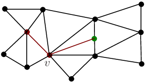
Obviously, we know that the vertex is the central vertex of Figure 13 and the red and green vertices and red edges are CCS then we know that by the coloring of Algorithm 3.
Figure 11 is a MOP with diameter where the Maximal fan structures having vertices and the red vertices and edges give the CCS When the Fan structures are replaced by any with the resulting graphs can be rainbow colored by
colors with the same method as Figure 11 showing. If we color the graph by the Maximal fan partition method, then the colors needed increase to 9 with the rising of
Definition (Two-way dominating set). A dominating set in a graph is called
a two-way dominating set, if every pendant vertex of is included in In addition,
if is connected, we call a connected two-way dominating set.
Theorem If is a connected two-way dominating set in a graph then
By the two-way dominating set and induction on radius, they proved the following result:
Theorem If is a bridge-less chordal graph, then Moreover,
there exists a bridge-less chordal graph with
For Figure 13, the minimum connected two-way dominating set is a path, thus by the theorem 5.3.
Another example Figure 9, we know that Figure 9 is a MOP, obviously a chordal graph, and has a hamiltonian cycle with vertices. By Theorem 1.1, we know that It is smaller than it’s and bigger 2 than it’s diameter.
If a MOP is then Therefor the upper bound of the algorithm given is sharp for MOPs, so is the Teorem 5.3. But above all, the bound gived by our algorithm is better to the theorem 5.3 obtained for some MOPs. For example, Figure 9 showing.
6 Concluding remarks
Recall algorithm 1, we know that the MOPs and with diameter have rainbow connection number Producing the graphs and giving their strong rainbow connection numbers take time at most
In algorithm 2: The Hamiltonian cycle of MOP can be obtained by a linear time algorithm presented in [24] through the canonical representation of Then select any vertex of as the initial vertex of we can obtain a Hamiltonian degree sequence in time where Note the time of Step 2 is where and which is Step 3 takes time at most and Step 4 at most For MOP, Step 5 takes time which is Step 6 at most
For algorithm 3: The time of Step 3 is no more than Step 4 uses time at most If is a MOP, the algorithm gives a tight upper bound of which is no more than where and needs time at most
In the future, we will consider the rainbow connection numbers for outerplanar and general planar graphs on algorithm aspect.
It is interesting to study the rainbow connection for planar graphs on algorithm aspect.
References
- [1] M. Basavaraju, L. S. Chandran, D. Rajendraprasad, and A. Ramaswamy. Rainbow connection number and radius, Graphs Combin., 30(2)(2014), 275-2852010.
- [2] L. Beineke and R. Pippert, A census of ball and disk dissections, Graph Theory and Applications (Proc. Conf., Western Michigan Univ., Kalamazoo, Mich., 1972), 25-40, Lect. Notes. Math., 303, Springer, 1972.
- [3] T. Beyer, W. Jones and S. Mitchell, Linear algorithms for isomorphism of maximal outerplanar graphs, J. Assoc. Comput. Mach., 26(4) (1979), 603-610.
- [4] Chang, G.J. and Nemhauser, G.L.: The k-domination and k-stability problems on graphs, SIAM J. Algebraic Discrete Meth., 5 (1984),332-345.
- [5] X. Deng, K. Xiang, B. Wu, Polynomial algorithm for sharp upper bound of rainbow connection number of maximal outerplanar graphs, Appl. Math. Lett., 25 (2012), 237-244.
- [6] X. Deng, H. Song,G.Su,W.Yang,R. Tian, Rainbow connection of bridgeless outerplanar graphs with small diameter, submitted.
- [7] Ananth, Prabhanjan, Meghana Nasre, and Kanthi K. Sarpatwar. Rainbow connectivity: hardness and tractability, LIPIcs-Leibniz International Proceedings in Informatics. 13, Schloss Dagstuhl-Leibniz-Zentrum fuer Informatik, 2011.
- [8] A. Farley and A. Proskurowski, Computation of the center and diameter of outerplanar graphs, Discrete Appl. Math., 2 (1980), 185-191.
- [9] H. L. Bodlaender, A linear time algorithm for finding tree decompositions of small treewidth, SIAM J. Comput., 25 (1996), 1305-1317.
- [10] Y. Caro, A. Lev, Y. Roditty, Z. Tuza and R. Yuster, On rainbow connection, Electron J. Combin. 15 (2008), R57.
- [11] S. Chakraborty, E. Fischer, A. Matsliah and R. Yuster, Hardness and algorithms for rainbow connectivity, J. Comb. Optim. 21(3) (2011), 330-347.
- [12] G. Chartrand, F. Harary, Planar permutation graphs, Ann. Inst. Henri Poincaré B., 3 (1967), 433-438.
- [13] L. S. Chandran, A. Das, D. Rajendraprasad, and N. M. Varma, Rainbow connection number and connected dominating sets, Electronic Notes in Discrete Math. 38(2011), 239-244. Also see J. Graph Theory. 71(2012), 206-218.
- [14] G. Chartrand, G. L. Johns, K. A. McKeon, and P. Zhang Rainbow connection in graphs, Math. Bohemica, 133 (2008) 85-98.
- [15] G. Hopkins, W. Staton, Outerplanarity without topology, Bull. Inst. Comb. Appl., 21 (1997), 112-116.
- [16] J. Kleinberg and É. Tardos, Algorithm design, John Wiley & Sons, Inc., 2002.
- [17] W. J. Cook, W. H. Cunningham, W. R. Pulleyblank, A. Schrijver, Combinatorial optimization, John Wiley Sons, Inc, 1998.
- [18] J. Ekstein, P. Holub, T. Kaiser, M. Koch, S.M. Camacho, Z. Ryj¡äacek, and I. Schier- meyer. The rainbow connection number of 2-connected graphs. Discrete Math., 2012. doi:10.1016/j.disc.2012.04.022.
- [19] J. Lauri, Further Hardness Results on Rainbow and Strong Rainbow Connectivity, Discrete Appl. Math., 201(11) (2016), 191-200.
- [20] X. Li, S.Liu, L.S. Chandran, R.Mathew and D.Rajendraprasad, Rainbow connection numbers and connectivity, Electron.J. Combin., 19:P20,2012.
- [21] H. Li, X. Li, and S. Liu, Rainbow connection of graphs with diameter 2, Discrete Mathematics, 312 (2012), 1453-1457.
- [22] H. Li, X. Li, and Y. Sun, Upper bound for the rainbow connection number of bridgeless graphs with diameter 3, arXiv: 1109.2769v2 [mathCO] 2011.
- [23] X. Li, Y. Shi, and Y. Sun, Rainbow connections of graphs: a survey, Graphs Combin., 29 (2013), 1-38.
- [24] S. Mitchell, Algorithms on trees and maximal outerplanar graphs: design, complexity analysis, and data structures study, PhD Thesis, University of Virginia, Charlottesville, VA, USA, 1977.
- [25] X. Huang, X. Li, Y. Shi, Note on the hardness of rainbow connections for planar and line graphs, Bull. Malays. Math. Sci. Soc., 38(3) (2015),1235-1241.
- [26] X. Huang, H. Li, X. Li, Y.Sun,Oriented diameter and rainbow connection number of a graph, DMTCS, 16(3)(2014), 51¨C60.
- [27] L.S. Chandran, A. Das, D. Rajendraprasad, N. Varma, Rainbow connection number and connected dominating sets, Electronic Notes in Discrete Math., 38(2011), 239¨C244. Also see J. Graph Theory, 71(2012), 206-218.
- [28] I. Schiermeyer, Rainbow connection in graphs with minimum degree three, IWOCA, LNCS, 5874 (2009), 432-437.
- [29] K. Uchizawa, T. Aoki, T. Ito, A. Suzuki, X. Zhou, On the rainbow connectivity of graphs: complexity and FPT algorithms, COCOON 2011,LNCS 6842(2011), 86-97.
- [30] D. B. West, Introduction to graph theory (second edition), Prentice Hall, NJ, 2001.