跳到论文正文
W Papers独立论文阅读器 arXiv:1605.01841 论文正文 计算阅读时间 · 0%
引用这篇论文根据当前论文元数据生成,正式投稿前建议核对。


License: arXiv.org perpetual non-exclusive license
arXiv:1605.01841v3 [hep-th] 21 Apr 2017

Gluon bound state and asymptotic freedom derived from the Bethe–Salpeter equation

Hitoshi Fukamachi Email: fukamachi-ht@kaiseigakuen.jp Affiliation: Kaisei Senior and Junior High Schools, Tokyo 116-0013, Japan    Kei-Ichi Kondo Email: kondok@faculty.chiba-u.jp Email: shogo.nishino@chiba-u.jp Email: sinohara@graduate.chiba-u.jp Affiliation: Department of Physics, Chiba University, Chiba 263-8522, Japan    Shogo Nishino    Toru Shinohara
Abstract

In this paper we study the two-body bound states for gluons and ghosts in a massive Yang-Mills theory which is obtained by generalizing the ordinary massless Yang-Mills theory in a manifestly Lorentz covariant gauge. First, we give a systematic derivation of the coupled Bethe-Salpeter equations for gluons and ghosts by using the Cornwall-Jackiw-Tomboulis effective action of the composite operators within the framework of the path integral quantization. Then, we obtain the numerical solutions for the Bethe-Salpeter amplitude representing the simultaneous bound states of gluons and ghosts by solving the homogeneous Bethe-Salpeter equation in the ladder approximation. We study how the inclusion of ghosts affects the two-gluon bound states. Moreover, we show explicitly that the approximate solutions obtained for the gluon-gluon amplitude are consistent with the ultraviolet asymptotic freedom signaled by the negative β\beta function.

PTEP-subject
12.38.Aw, 21.65.Qr
††preprintnumber: CHIBA-EP-218

1 Introduction

As is well known, the basic ingredients relevant to the strong interactions are quarks and gluons to be described by quantum chromodynamics (QCD). However, we believe that they are confined and never observed in their isolated form and that only the color-singlet composite particles such as mesons, baryons and glueballs consisted of quarks and gluons can be observed in experiments. In particular, glueballs were predicted in the middle of the 1970s by Fritzsch and Minkowski [1], in contrast to mesons and baryons to be explained by the quark model proposed by Gell-Mann in the middle of the 1960s [2]. Since then, the properties of glueballs have been investigated in various theoretical frameworks and also by experiments.

The equation for describing the bound states in the framework of the relativistic quantum field theory is known as the Nambu-Bethe–Salpeter equation or the Bethe–Salpeter (BS) equation [3, 4]. The BS equation is a self-consistent equation written in terms of the BS amplitude as the wave function of the bound state. See e.g., [5] for reviews. The BS equation is specified for a given set of propagators and the interaction vertex functions describing the constituent particles. In the non-perturbative framework, propagators and vertex functions can be obtained by solving the Schwinger-Dyson (SD) equation which is a self-consistent equation written in terms of propagators and vertex functions for the fundamental fields in a given field theory. In order to describe the bound state in the non-perturbative framework, therefore, we must take into account the SD equation and the BS equation simultaneously: The SD equation must be solved to give propagators and vertex functions as inputs for specifying the BS equation. Then the BS equation is to be solved in the same level of approximations as those used in solving the SD equation, as far as they cannot be solved exactly.

The purpose of this paper is to understand glueball formation from the underlying dynamics of the Yang-Mills theory in a way consistent with confinement and ultraviolet asymptotic freedom. In order to avoid complications arising from the mixing of glueballs with mesons in QCD, we restrict our consideration to the pure glue dynamics, namely, pure Yang-Mills theory. Therefore, a glueball is supposed to be a bound state of gluons. In this paper, especially, we study a glueball as a two-gluon bound state for simplifying the treatment.

Already in the late 1970s, Fukuda [6] studied a two-body bound state of gluons and ghosts as solution of the BS equation in the ladder approximation in the framework of the Yang-Mills theory with the covariant gauge fixing. He has shown the existence of the tachyon bound state due to the dominating attractive force between two gauge (gluon) particles in the color singlet and spin singlet channel, for whatever small coupling constant. The gauge particles interact among themselves through a three-gluon interaction and a contact four-gluon interaction, and interact with ghosts through the gluon-ghost interaction due to the covariant gauge fixing. The three-gluon interaction gives an attractive force between two gauge particles in the color singlet channel by exchanging a gauge particle (This is the analog of the attraction of opposite charge in the Abelian gauge theory). While the contact four-gluon interaction produces a repulsive force. However, if the attraction due to former dominates the repulsion from the latter, the two gauge particles can form a bound state by the net attractive force. This is nothing but a pairing phenomena familiar in the BCS theory of superconductivity. Since gauge particles are massless, however, the resulting bound state should necessarily correspond to a tachyon pole. However, his observations play the very important role for obtaining glueballs consisted of massive gluons in this paper. It was also shown [7] that such a tachyonic bound state continues to exist even in the presence of nn flavors of quarks and gluons acquire a mass due to vacuum rearrangement, when nn is smaller than or equal to a critical value ncn_{c}, n≤ncn\leq n_{c}, while all particles remain massless for n>ncn>n_{c}.

In the classical level, indeed, the Yang-Mills theory in the four-dimensional spacetime is a massless theory with no scale. In the quantum level, however, the Yang-Mills theory should have a mass scale as suggested from the dimensional transmutation and could have the mass gap. Recently, a solution corresponding to a confining gluon of the massive type was discovered as a solution of the coupled SD equation for the gluon and ghost propagators in the S​U​(N)SU(N) Yang-Mills theory with the Landau gauge fixing, which is called the decoupling solution [8], in sharp contrast to the scaling solution [9]. The existence of the decoupling solution is supported and its confining properties are investigated by various analytical and numerical frameworks. However, it is not yet clear how to understand the decoupling solution as a solution to be consistent with gluon confinement and more general color confinement, see e.g., [10].

The Brout-Englert-Higgs mechanism is accepted as a unique way for providing the mass for gauge bosons in quantum field theories, because it is the only one established method which enables one to maintain both renormalizability and physical unitarity. In this paper, we consider a specific model including a mass term for the Yang-Mills field, which is a special case of the Curci-Ferrari model [11]. We call this model the massive Yang-Mills theory for later convenience. We adopt this model to perform the analytical investigation for gluons of massive type, instead of using the decoupling solution obtained by solving the SD equation, since the decoupling solution has been so far obtained only in a numerical way, and the analytical expression for the decoupling solution is not yet known explicitly.

We started our analysis on massive Yang-Mills theory in the previous papers [12] without introducing the Higgs field which causes the Higgs mechanism. Nevertheless, we are not plagued by the unitarity violation in high energy region of the massive Yang-Mills theory without the Higgs scalar. This is because we regard our massive Yang-Mills theory just as a low-energy effective theory (valid below a certain cutoff Λ\Lambda) of the quantum Yang-Mills theory with mass gap and confinement. To mimic precisely the decoupling solution, we must introduce the momentum-dependent gluon mass m⁡(p)m(p) which vanishes in the high-energy region and remains non-zero in the low-energy region. In this paper, we have adopted a constant mass mm valid up to a momentum cutoff Λ\Lambda to simplify the analyses without assuming the specific function of the momentum pp. Our standpoint mentioned above has been already given more explicitly in the second paper of [12] and is not repeated here.

It is also known that this model of massive Yang-Mills theory is still renormalizable, but loses the physical unitarity as least in the perturbation theory [12]. We leave the issue how to realize it as a sound model in a quantum field theoretical framework. We have a hope that this issue will be resolved in a non-perturbative framework. One of the motivation of this paper is to obtain some information towards this direction to consider bound states in a massive Yang-Mills theory without the Higgs field as a low-energy effective theory of QCD.

The issue of a tachyon bound state will be avoided by starting from the massive Yang-Mills particles instead of the massless gauge particles. Consequently, we will obtain the massive bound states consisted of two massive gluons described by the massive Yang-Mills theory. In obtaining such a solution, especially, we pay special attention to the aspect how our results for the bound state is consistent with the ultraviolet asymptotic freedom [13]. This is a feature that has not been discussed in the preceding works [14, 15]. In their works, the precise determinations of the glueball spectrum have been the main purpose of investigations. Such an issue is not the aim of the present paper, although it is a nice goal of future investigations to be achieved by developing our method.

We give a systematic derivation of the coupled BS equation for gluon and ghost by starting from the the Cornwall-Jackiw-Toumboulis effective (CJT) action for the composite operator with the bilocal source term. We show that the bound state obtained as a solution of the homogeneous BS equation for the gluon-gluon BS amplitude is consistent with the ultraviolet asymptotic freedom.

This paper is organized as follows. In sec. II, we introduce the massive Yang-Mills theory from which we start the study of the bound state. In section III, we give the CJT effective action for the bilocal composite operator, which gives a systematic derivation of the BS equation. In sec. IV, we derive the BS equation by differentiating the CJT effective action with respect to the full Green functions. In sec. V, we write down the coupled BS equation for gluon and ghost at vanishing total momentum P=0P=0 in the massless case, and obtain the numerical solutions. This is a preliminary study of obtaining the bound state. In sec. VI, we write down the homogeneous BS equation at the general total momentum PP in the massive case, but restricting to the gluon-gluon BS amplitude alone. In sec. VII, we solve the BS equation for the gluon-gluon BS amplitude at the general total momentum PP in the massive case. The final section is devoted to conclusion and discussion. Some technical materials are collected in the Appendices.

2 The massive Yang-Mills theory

In order to discuss the bound state, we adopt the massive S​U​(N)SU(N) Yang-Mills theory without the Higgs field, which is defined to be the usual massless S​U​(N)SU(N) Yang-Mills theory in the most general Lorenz gauge [16] plus the “mass term” ℒm\mathscr{L}_{m} formulated in a manifestly Lorentz covariant way. The total Lagrangian density ℒm​YMtot\mathscr{L}^{\rm{tot}}_{m\rm{YM}} is written in terms of the Yang-Mills field 𝒜μ\mathscr{A}_{\mu}, the Faddeev-Popov ghost field 𝒞\mathscr{C}, the antighost field 𝒞¯\bar{\mathscr{C}} and the Nakanishi-Lautrup auxiliary field 𝒩\mathscr{N}, if we use the terminology adopted in the usual massless Yang-Mills theory:

ℒm​YMtot=\displaystyle\mathscr{L}^{\rm{tot}}_{m\rm{YM}}= ℒYM+ℒGF+FP+ℒm,\displaystyle\mathscr{L}_{\rm{YM}}+\mathscr{L}_{\rm{GF+FP}}+\mathscr{L}_{m}, (1a)
ℒYM=\displaystyle\mathscr{L}_{\rm{YM}}= −14ℱμ​ν⋅ℱμ​ν,\displaystyle-\frac{1}{4}\mathscr{F}_{\mu\nu}\cdot\mathscr{F}^{\mu\nu}, (1b)
ℒGF+FP=\displaystyle\mathscr{L}_{\rm{GF+FP}}= 𝒩⋅∂μ𝒜μ+i​𝒞¯⋅∂μ𝒟μ​[𝒜]​𝒞+β4​(𝒩¯⋅𝒩¯+𝒩⋅𝒩)+α2​𝒩⋅𝒩\displaystyle\mathscr{N}\cdot\partial^{\mu}\mathscr{A}_{\mu}+i\bar{\mathscr{C}}\cdot\partial^{\mu}\mathscr{D}_{\mu}[\mathscr{A}]\mathscr{C}+\frac{\beta}{4}(\bar{\mathscr{N}}\cdot\bar{\mathscr{N}}+\mathscr{N}\cdot\mathscr{N})+\frac{\alpha}{2}\mathscr{N}\cdot\mathscr{N}
=\displaystyle= α2​𝒩⋅𝒩+β2​𝒩⋅𝒩+𝒩⋅∂μ𝒜μ−β2​g​𝒩⋅(i​𝒞¯×𝒞)\displaystyle\frac{\alpha}{2}\mathscr{N}\cdot\mathscr{N}+\frac{\beta}{2}\mathscr{N}\cdot\mathscr{N}+\mathscr{N}\cdot\partial^{\mu}\mathscr{A}_{\mu}-\frac{\beta}{2}g\mathscr{N}\cdot(i\bar{\mathscr{C}}\times\mathscr{C})
+i𝒞¯⋅∂μ𝒟μ[𝒜]𝒞+β4g2(i𝒞¯×𝒞)⋅(i𝒞¯×𝒞),\displaystyle+i\bar{\mathscr{C}}\cdot\partial^{\mu}\mathscr{D}_{\mu}[\mathscr{A}]\mathscr{C}+\frac{\beta}{4}g^{2}(i\bar{\mathscr{C}}\times\mathscr{C})\cdot(i\bar{\mathscr{C}}\times\mathscr{C}), (1c)
ℒm=\displaystyle\mathscr{L}_{m}= 12​m2​𝒜μ⋅𝒜μ+β​m2​i​𝒞¯⋅𝒞,\displaystyle\frac{1}{2}m^{2}\mathscr{A}_{\mu}\cdot\mathscr{A}^{\mu}+\beta m^{2}i\bar{\mathscr{C}}\cdot\mathscr{C}, (1d)

where 𝒟μ\mathscr{D}_{\mu} is the covariant derivative defined by

𝒟μ​[𝒜]​ω​(x):=∂μω⁡(x)+g​𝒜μ​(x)×ω⁡(x),\displaystyle\mathscr{D}_{\mu}[\mathscr{A}]\omega(x):=\partial_{\mu}\omega(x)+g\mathscr{A}_{\mu}(x)\times\omega(x), (2)

and 𝒩¯\bar{\mathscr{N}} is defined by

𝒩¯:=−𝒩+g​i​𝒞¯×𝒞.\bar{\mathscr{N}}:=-\mathscr{N}+gi\bar{\mathscr{C}}\times\mathscr{C}. (3)

Here we have adopted the notation:

𝒳⋅𝒴:=\displaystyle\mathscr{X}\cdot\mathscr{Y}:= 𝒳a​𝒴a,(𝒳×𝒴)c:=fa​b​c​𝒳a​𝒴b,\displaystyle\mathscr{X}^{a}\mathscr{Y}^{a},\quad(\mathscr{X}\times\mathscr{Y})^{c}:=f_{abc}\mathscr{X}^{a}\mathscr{Y}^{b}, (4)

where fa​b​cf_{abc} is the structure constants of the Lie algebra of the S​U​(N)SU(N) group. Here α\alpha and β\beta are parameters which are identified with the gauge-fixing parameters in the m→0m\rightarrow 0 limit. The α=0\alpha=0 case is the Curci-Ferrari model [11] with the coupling constant gg, the mass parameter mm and the parameter β\beta. In the Abelian limit with vanishing structure constants fa​b​c=0f_{abc}=0, the Faddeev-Popov ghosts decouple and the Curci-Ferrari model reduces to the Nakanishi model [17].

In what follows, we put β=0\beta=0 to simulate the decoupling solution representing massive gluon and massless ghost. By eliminating the Nakanishi-Lautrup field 𝒩\mathscr{N}, ℒm​YMtot\mathscr{L}^{\rm{tot}}_{m\rm{YM}} reads

ℒm​YMtot=\displaystyle\mathscr{L}^{\rm{tot}}_{m\rm{YM}}= −14(∂μ𝒜ν−∂ν𝒜μ)⋅(∂μ𝒜ν−∂ν𝒜μ)−12​α(∂μ𝒜μ)2+i𝒞¯⋅□𝒞\displaystyle-\frac{1}{4}(\partial_{\mu}\mathscr{A}_{\nu}-\partial_{\nu}\mathscr{A}_{\mu})\cdot(\partial^{\mu}\mathscr{A}^{\nu}-\partial^{\nu}\mathscr{A}^{\mu})-\frac{1}{2\alpha}\left(\partial^{\mu}\mathscr{A}_{\mu}\right)^{2}+i\bar{\mathscr{C}}\cdot\Box\mathscr{C}
−12g(∂μ𝒜ν−∂ν𝒜μ)⋅(𝒜μ×𝒜ν)−14g2(𝒜μ×𝒜ν)2+gi𝒞¯⋅∂μ(𝒜μ×𝒞)\displaystyle-\frac{1}{2}g\left(\partial_{\mu}\mathscr{A}_{\nu}-\partial_{\nu}\mathscr{A}_{\mu}\right)\cdot\left(\mathscr{A}^{\mu}\times\mathscr{A}^{\nu}\right)-\frac{1}{4}g^{2}\left(\mathscr{A}_{\mu}\times\mathscr{A}_{\nu}\right)^{2}+gi\bar{\mathscr{C}}\cdot\partial^{\mu}\left(\mathscr{A}_{\mu}\times\mathscr{C}\right)
+12m2𝒜μ⋅𝒜μ.\displaystyle+\frac{1}{2}m^{2}\mathscr{A}_{\mu}\cdot\mathscr{A}^{\mu}. (5)

By starting from the massive Yang-Mills theory given by the Lagrangian density (5), we derive the BS equation which includes simultaneously gluon and ghost on equal footing. This can be done using the CJT effective action for the composite operators, as explicitly shown in [13]. See [12] for more details on this model.

3 Cornwall–Jackiw–Tomboulis effective action

For the Yang–Mills theory, we introduce the local sources Jaμ​(x)J^{\mu}_{a}(x), η¯a​(x)\bar{\eta}_{a}(x), and ηa​(x)\eta_{a}(x) for the gluon field 𝒜μa​(x)\mathscr{A}_{\mu}^{a}(x), the ghost field 𝒞a​(x)\mathscr{C}^{a}(x), and the antighost field 𝒞¯a​(x)\mathscr{\bar{C}}^{a}(x) respectively. Moreover, we introduce the bilocal sources Ia​bμ​ν​(x,y)I_{ab}^{\mu\nu}(x,y) and θa​b​(x,y)\theta_{ab}(x,y) for the bilocal composite operators 𝒜μa​(x)​𝒜νb​(y)\mathscr{A}_{\mu}^{a}(x)\mathscr{A}_{\nu}^{b}(y) and 𝒞¯a​(x)​𝒞b​(y)\mathscr{\bar{C}}^{a}(x)\mathscr{C}^{b}(y) respectively, where the bilocal source II is symmetric Iμ​νa​b​(x,y)=Iν​μb​a​(y,x)I^{ab}_{\mu\nu}(x,y)=I^{ba}_{\nu\mu}(y,x) and θa​b​(x,y)\theta^{ab}(x,y) is a general matrix. Then the generating functional W⁡[J,η¯,η,I,θ]W[J,\bar{\eta},\eta,I,\theta] is defined by

Z⁡[J,η¯,η,I,θ]=ei​W​[J,η¯,η,I,θ]\displaystyle Z[J,\bar{\eta},\eta,I,\theta]=e^{iW[J,\bar{\eta},\eta,I,\theta]}
=\displaystyle= ∫𝒟Φexp{iSm​YMtot[𝒜,𝒞¯,𝒞]+i∫x[Jaμ(x)𝒜μa(x)+η¯a(x)𝒞a(x)+𝒞¯a(x)ηa(x)]\displaystyle\int\mathcal{D}\Phi\exp\Bigg\{iS^{\rm{tot}}_{m\rm{YM}}[\mathscr{A},\mathscr{\bar{C}},\mathscr{C}]+i\int_{x}\left[J^{\mu}_{a}(x)\mathscr{A}_{\mu}^{a}(x)+\bar{\eta}_{a}(x)\mathscr{C}^{a}(x)+\mathscr{\bar{C}}^{a}(x)\eta_{a}(x)\right]
+i∫x∫y[12𝒜μa(x)Ia​bμ​ν(x,y)𝒜νb(y)+𝒞¯a(x)θa​b(x,y)𝒞b(y)]},\displaystyle\hskip 85.35826pt+i\int_{x}\int_{y}\left[\frac{1}{2}\mathscr{A}^{a}_{\mu}(x)I_{ab}^{\mu\nu}(x,y)\mathscr{A}^{b}_{\nu}(y)+\mathscr{\bar{C}}^{a}(x)\theta_{ab}(x,y)\mathscr{C}^{b}(y)\right]\Bigg\}, (6)

where we have introduced the abbreviated notation: ∫x:=∫dDx\int_{x}:=\int d^{D}x. For the local source, we find that the (left) derivatives of WW with respect to the local sources are given by

δ​Wδ​Jaμ​(x)\displaystyle\frac{\delta W}{\delta J_{a}^{\mu}(x)} =⟨𝒜μa​(x)⟩≡𝑨μa​(x),\displaystyle=\left<\mathscr{A}^{a}_{\mu}(x)\right>\equiv\bm{A}_{\mu}^{a}(x), (7a)
δ​Wδ​η¯a​(x′)\displaystyle\quad\frac{\delta W}{\delta\bar{\eta}_{a}(x^{\prime})} =⟨𝒞a​(x′)⟩≡𝑪a​(x′),δ​Wδ​ηa​(x′)=−⟨𝒞¯a​(x′)⟩≡−𝑪¯a​(x′),\displaystyle=\left<\mathscr{C}^{a}(x^{\prime})\right>\equiv\bm{C}^{a}(x^{\prime}),\quad\frac{\delta W}{\delta\eta_{a}(x^{\prime})}=-\left<\mathscr{\bar{C}}^{a}(x^{\prime})\right>\equiv-\bar{\bm{C}}^{a}(x^{\prime}), (7b)
δ2​Wδ​Jbν​(y)​δ​Jaμ​(x)\displaystyle\frac{\delta^{2}W}{\delta J^{\nu}_{b}(y)\delta J_{a}^{\mu}(x)} =i⁡⟨𝒜μa​(x);𝒜νb​(y)⟩≡i​Dμ​νa​b​(x,y),\displaystyle=i\left<\mathscr{A}^{a}_{\mu}(x);\mathscr{A}^{b}_{\nu}(y)\right>\equiv iD^{ab}_{\mu\nu}(x,y), (7c)
δ2​Wδ​ηb​(y′)​δ​η¯a​(x′)\displaystyle\frac{\delta^{2}W}{\delta\eta_{b}(y^{\prime})\delta\bar{\eta}_{a}(x^{\prime})} =i⁡⟨𝒞a​(x′);𝒞¯b​(y′)⟩≡i​Δa​b​(x′,y′),\displaystyle=i\left<\mathscr{C}^{a}(x^{\prime});\mathscr{\bar{C}}^{b}(y^{\prime})\right>\equiv i\Delta^{ab}(x^{\prime},y^{\prime}), (7d)
δ2​Wδ​η¯b​(y′)​δ​ηa​(x′)\displaystyle\frac{\delta^{2}W}{\delta\bar{\eta}_{b}(y^{\prime})\delta\eta_{a}(x^{\prime})} =i⁡⟨𝒞¯a​(x′);𝒞b​(y)⟩≡i​Δ~a​b​(x′,y′),\displaystyle=i\left<\mathscr{\bar{C}}^{a}(x^{\prime});\mathscr{C}^{b}(y)\right>\equiv i\tilde{\Delta}^{ab}(x^{\prime},y^{\prime}), (7e)

where DD and Δ~\tilde{\Delta} are the full gluon and ghost-antighost propagators.

For the bilocal source, we find that the derivatives of WW with respect to the bilocal sources are given by

δ​Wδ​Ia​bμ​ν​(x,y)\displaystyle\frac{\delta W}{\delta I_{ab}^{\mu\nu}(x,y)} =⟨𝒜μa​(x)​𝒜νb​(y)⟩=⟨𝒜μa​(x);𝒜νb​(y)⟩+⟨𝒜μa​(x)⟩​⟨𝒜νb​(y)⟩\displaystyle=\left<\mathscr{A}_{\mu}^{a}(x)\mathscr{A}_{\nu}^{b}(y)\right>=\left<\mathscr{A}_{\mu}^{a}(x);\mathscr{A}_{\nu}^{b}(y)\right>+\left<\mathscr{A}_{\mu}^{a}(x)\right>\left<\mathscr{A}_{\nu}^{b}(y)\right>
=Dμ​νa​b​(x,y)+𝑨μa​(x)​𝑨νb​(y),\displaystyle=D_{\mu\nu}^{ab}(x,y)+\bm{A}_{\mu}^{a}(x)\bm{A}_{\nu}^{b}(y), (8a)
δ​Wδ​θa​b​(x′,y′)\displaystyle\frac{\delta W}{\delta\theta_{ab}(x^{\prime},y^{\prime})} =⟨𝒞¯a​(x′)​𝒞b​(y′)⟩=⟨𝒞¯a​(x′);𝒞b​(y′)⟩+⟨𝒞¯a​(x′)⟩​⟨𝒞b​(y′)⟩\displaystyle=\left<\mathscr{\bar{C}}^{a}(x^{\prime})\mathscr{C}^{b}(y^{\prime})\right>=\left<\mathscr{\bar{C}}^{a}(x^{\prime});\mathscr{C}^{b}(y^{\prime})\right>+\left<\mathscr{\bar{C}}^{a}(x^{\prime})\right>\left<\mathscr{C}^{b}(y^{\prime})\right>
=Δ~a​b​(x′,y′)+𝑪¯a​(x′)​𝑪b​(y′).\displaystyle=\tilde{\Delta}^{ab}(x^{\prime},y^{\prime})+\bar{\bm{C}}^{a}(x^{\prime})\bm{C}^{b}(y^{\prime}). (8b)

We define the CJT effective action [18] of the Yang-Mills theory by the Legendre transform:

Γ⁡[𝑨,𝑪¯,𝑪,D,Δ~]=\displaystyle\Gamma[\bm{A},\bar{\bm{C}},\bm{C},D,\tilde{\Delta}]= W⁡[J,η¯,η,I,θ]−∫x(Jaμ​(x)​𝑨μa​(x)+η¯a​(x)​𝑪a​(x)+𝑪¯a​(x)​ηa​(x))\displaystyle W[J,\bar{\eta},\eta,I,\theta]-\int_{x}\left(J_{a}^{\mu}(x)\bm{A}^{a}_{\mu}(x)+\bar{\eta}_{a}(x)\bm{C}^{a}(x)+\bar{\bm{C}}^{a}(x)\eta_{a}(x)\right)
−12∫x∫y(𝑨μa(x)Ia​bμ​ν(x,y)𝑨νb(y)+Ia​bμ​ν(x,y)Dμ​νa​b(x,y))\displaystyle-\frac{1}{2}\int_{x}\int_{y}\left(\bm{A}^{a}_{\mu}(x)I_{ab}^{\mu\nu}(x,y)\bm{A}^{b}_{\nu}(y)+I_{ab}^{\mu\nu}(x,y)D^{ab}_{\mu\nu}(x,y)\right)
−∫x′∫y′(𝑪¯a(x′)θa​b(x′,y′)𝑪b(y′)+θa​b(x′,y′)Δ~a​b(x′,y′)).\displaystyle-\int_{x^{\prime}}\int_{y^{\prime}}\left(\bar{\bm{C}}^{a}(x^{\prime})\theta_{ab}(x^{\prime},y^{\prime})\bm{C}^{b}(y^{\prime})+\theta_{ab}(x^{\prime},y^{\prime})\tilde{\Delta}^{ab}(x^{\prime},y^{\prime})\right). (9)

Then we find the derivatives of Γ\Gamma with respect to the field expectation,

δ​Γδ​𝑨μa​(x)\displaystyle\frac{\delta\Gamma}{\delta\bm{A}_{\mu}^{a}(x)} =−Jaμ​(x)−∫yIa​bμ​ν​(x,y)​𝑨νb​(y),\displaystyle=-J^{\mu}_{a}(x)-\int_{y}I_{ab}^{\mu\nu}(x,y)\bm{A}_{\nu}^{b}(y), (10a)
δ​Γδ​𝑪¯a​(x′)\displaystyle\frac{\delta\Gamma}{\delta\bar{\bm{C}}^{a}(x^{\prime})} =−ηa​(x′)−∫y′θa​b​(x′,y′)​𝑪b​(y′),δ​Γδ​𝑪b​(y′)=η¯b​(y′)+∫y′𝑪¯a​(x′)​θa​b​(x′,y′),\displaystyle=-\eta_{a}(x^{\prime})-\int_{y^{\prime}}\theta_{ab}(x^{\prime},y^{\prime})\bm{C}^{b}(y^{\prime}),\quad\frac{\delta\Gamma}{\delta\bm{C}^{b}(y^{\prime})}=\bar{\eta}_{b}(y^{\prime})+\int_{y^{\prime}}\bar{\bm{C}}^{a}(x^{\prime})\theta_{ab}(x^{\prime},y^{\prime}), (10b)
and the derivatives of Γ\Gamma with respect to the full propagators,
δ​Γδ​Dμ​νa​b​(x,y)\displaystyle\frac{\delta\Gamma}{\delta D_{\mu\nu}^{ab}(x,y)} =−Ia​bμ​ν​(x,y),δ​Γδ​Δ~a​b​(x′,y′)=−θa​b​(x′,y′).\displaystyle=-I^{\mu\nu}_{ab}(x,y),\quad\frac{\delta\Gamma}{\delta\tilde{\Delta}^{ab}(x^{\prime},y^{\prime})}=-\theta_{ab}(x^{\prime},y^{\prime}). (10c)

It is shown that the CJT effective action is rewritten as

Γ⁡[𝑨,𝑪,𝑪¯,D,Δ~]=\displaystyle\Gamma[\bm{A},\bm{C},\bar{\bm{C}},D,\tilde{\Delta}]= Sm​YMtot​[𝑨,𝑪,𝑪¯]+i2​Tr​[𝒟A​A−1​D]−i​Tr​[𝒟¯C​C¯−1​Δ~]\displaystyle S^{\rm{tot}}_{m\rm{YM}}[\bm{A},\bm{C},\bar{\bm{C}}]+\frac{i}{2}{\text{Tr}}\left[\mathscr{D}^{-1}_{AA}D\right]-i{\text{Tr}}\left[\bar{\mathscr{D}}^{-1}_{C\bar{C}}\tilde{\Delta}\right]
+i2​Tr​ln⁡D−1+i​Tr​ln⁡Δ~−1+Γ2​[𝑨,𝑪,𝑪¯,D,Δ~],\displaystyle+\frac{i}{2}{\text{Tr}}\ln D^{-1}+i{\text{Tr}}\ln\tilde{\Delta}^{-1}+\Gamma_{2}[\bm{A},\bm{C},\bar{\bm{C}},D,\tilde{\Delta}], (11)

where Γ2\Gamma_{2} is the two particle irreducible (2PI) contributions, DD and Δ~\tilde{\Delta} are respectively the full gluon and ghost propagators, 𝒟A​A\mathscr{D}_{AA} and 𝒟¯C​C¯\bar{\mathscr{D}}_{C\bar{C}} are respectively the tree-level gluon and ghost propagators defined by

δ2​𝑺δ​𝑨νb​(y)​δ​𝑨μa​(x)\displaystyle\frac{\delta^{2}\bm{S}}{\delta\bm{A}_{\nu}^{b}(y)\delta\bm{A}_{\mu}^{a}(x)} ≡(i​𝒟A​A−1)μ​νa​b​(x,y),δ2​𝑺δ​𝑪¯a​(x)​δ​𝑪b​(y)≡(i​𝒟¯C​C¯−1)a​b​(x,y).\displaystyle\equiv(i\mathscr{D}^{-1}_{AA})_{\mu\nu}^{ab}(x,y),\quad\frac{\delta^{2}\bm{S}}{\delta\bar{\bm{C}}^{a}(x)\delta\bm{C}^{b}(y)}\equiv(i\bar{\mathscr{D}}^{-1}_{C\bar{C}})^{ab}(x,y). (12)

The original Yang-Mills theory is characterized by the bare gluon and ghost propagators, and the bare one particle irreducible (1PI) vertex functions: 3-gluon, 4-gluon, and gluon-ghost-antighost vertices given in Fig. 1. The full gluon and ghost propagators, and the full 1PI vertex functions: 3-gluon, 4-gluon, and gluon-ghost-antighost vertices are given in Fig. 2. It is shown that the 2PI vacuum diagrams in the Yang-Mills theory are written as Fig. 3.

Refer to caption
Refer to caption
Figure 1: Bare gluon and ghost propagators; the bare vertex functions: 3-gluon, 4-gluon, gluon-ghost-antighost vertices in the Yang-Mills theory.
Refer to caption
Refer to caption
Figure 2: Full gluon and ghost propagators; the full vertex functions: 3-gluon, 4-gluon, gluon-ghost-antighost vertices in the Yang-Mills theory.
Refer to caption
Figure 3: 2PI vacuum diagrams in the Yang-Mills theory.

4 A systematic derivation of the Bethe–Salpeter equation

4.1 Derivation of the Schwinger–Dyson equation

By taking the first derivative of the CJT effective action Γ\Gamma with respect to the full gluon and ghost propagators DD, we obtain the SD equations for the gluon propagator DD and ghost propagator δ​Δ~\delta\tilde{\Delta} respectively (after the sources are setting to be zero I,θ→0I,\theta\to 0):

−I=δ​Γδ​D=−i​D−1+i​𝒟A​A−1+δ​Γ2δ​D,\displaystyle-I=\frac{\delta\Gamma}{\delta D}=-iD^{-1}+i\mathscr{D}_{AA}^{-1}+\frac{\delta\Gamma_{2}}{\delta D}, (13a)
−θ=δ​Γδ​Δ~​(x,y)=−i​Δ~−1+i​𝒟~C​C¯−1+δ​Γ2δ​Δ~.\displaystyle-\theta=\frac{\delta\Gamma}{\delta\tilde{\Delta}(x,y)}=-i\tilde{\Delta}^{-1}+i\tilde{\mathscr{D}}_{C\bar{C}}^{-1}+\frac{\delta\Gamma_{2}}{\delta\tilde{\Delta}}. (13b)

Fig. 5 is the gluon SD equation and Fig. 5 is the ghost SD equation.

Refer to caption
Figure 4: Gluon-SD equation.
Refer to caption
Figure 5: Ghost-SD equation.

4.2 The equation for the scattering Green function

The BS equation is obtained by taking the first derivative of the SD equation (i.e., the second derivative of the CJT effective action) with respect to the full propagator. For the general field ϕ\phi, the scattering Green function D4D_{4} with four external lines is defined by the second derivative of WW with respect to the bilocal source II:

D4​(x′,y′,x,y)=\displaystyle D_{4}(x^{\prime},y^{\prime};x,y)= ⟨0|​ϕ​(x)​ϕ​(y);ϕ⁡(x′)​ϕ​(y′)​|0⟩=1i​δ2​Wδ​I​(x′,y′)​δ​I​(x,y),\displaystyle\left<0|\phi(x)\phi(y);\phi(x^{\prime})\phi(y^{\prime})|0\right>=\frac{1}{i}\frac{\delta^{2}W}{\delta I(x^{\prime},y^{\prime})\delta I(x,y)}, (14)

while the inverse D4−1D_{4}^{-1} of the scattering Green function D4D_{4} is given by the second derivative of Γ\Gamma with respect to the full propagator DD:

D4−1:=δ2​Γδ​D​δ​D.\displaystyle D_{4}^{-1}:=\frac{\delta^{2}\Gamma}{\delta D\delta D}. (15)

Therefore, the first derivative of the SD equation yields the equation for the inverse D4−1D_{4}^{-1} of the scattering Green function D4D_{4}:

D4−1=D4(0)−1+K,D4(0)−1:=δ2​[−i​D−1]δ​D​δ​D,K:=δ2​Γ2δ​D​δ​D,\displaystyle D_{4}^{-1}=D_{4}^{(0)}{}^{-1}+K,\quad D_{4}^{(0)}{}^{-1}:=\frac{\delta^{2}[-iD^{-1}]}{\delta D\delta D},\quad K:=\frac{\delta^{2}\Gamma_{2}}{\delta D\delta D}, (16)

where D4(0)D_{4}^{(0)} is the tree part of the scattering Green function D4D_{4} and KK denotes the kernel. The diagrammatic representation is given as

[Uncaptioned image] (17)

We make use of the identities:

[Uncaptioned image]and[Uncaptioned image]\includegraphics[scale={0.30}]{fig-ep218/identity}\hskip 42.67912pt{\rm{and}}\hskip 42.67912pt\includegraphics[scale={0.30}]{fig-ep218/identity2} (18)

to rewrite the equation in terms of D4D_{4}, not the inverse D4−1D_{4}^{-1}. We multiply D4D_{4} from the right to obtain

[Uncaptioned image] (19)

and then multiply D4(0)D_{4}^{(0)} from the left to obtain

[Uncaptioned image] (20)

Thus we obtain the self-consistent equation for the scattering Green function D4D_{4} after multiplying ii:

[Uncaptioned image] (21)

For the Yang-Mills theory, we obtain a set of the BS equations for the four BS amplitude: gluon-gluon, gluon-ghost, ghost-gluon, and ghost-ghost scattering Green function as given in Fig. 6.

Refer to caption
Refer to caption
Figure 6: The BS equation for gluon-gluon DD, gluon-ghost GG, ghost-gluon GG, and ghost-ghost Δ\Delta scattering Green functions.

4.3 The homogeneous BS equation for the (amputated) BS amplitude

We can use the completeness relation:

𝟏=|0⟩⟨0|+∑c∫dd​𝑷c(2​π)d12​EPc|Pc⟩⟨Pc|+⋯,\bm{1}=|0\big>\big<0|+\sum_{c}\int\frac{d^{d}\bm{P}_{c}}{(2\pi)^{d}}\frac{1}{2E_{P_{c}}}|P_{c}\big>\big<P_{c}|+\cdots, (22)

where the sum ∑c\sum_{c} runs over all the bound states except for the continuum spectrum. The scattering Green function D4D_{4} for particles described by the field ϕa\phi_{a} is defined by

D4(x′,y′;x,y)a′​b′;a​b=\displaystyle D_{4}{}^{a^{\prime}b^{\prime};ab}(x^{\prime},y^{\prime};x,y)= ⟨0|​ϕa​(x)​ϕb​(y);ϕa′​(x′)​ϕb′​(y′)​|0⟩=1i​δ2​Wδ​Ia′​b′​(x′,y′)​δ​Ia​b​(x,y).\displaystyle\left<0|\phi^{a}(x)\phi^{b}(y);\phi^{a^{\prime}}(x^{\prime})\phi^{b^{\prime}}(y^{\prime})|0\right>=\frac{1}{i}\frac{\delta^{2}W}{\delta I^{a^{\prime}b^{\prime}}(x^{\prime},y^{\prime})\delta I^{ab}(x,y)}. (23)

This is decomposed into the product of the BS amplitude χ\chi:

D4(x′,y′;x,y)a′​b′;a​b=\displaystyle D_{4}{}^{a^{\prime}b^{\prime};ab}(x^{\prime},y^{\prime};x,y)= ∑c∫dd​Pc(2​π)d​12​EPc​χPa​b​(x,y)​χ¯Pa′​b′​(x′,y′)+…,\displaystyle\sum_{c}\int\frac{d^{d}P_{c}}{(2\pi)^{d}}\frac{1}{2E_{P_{c}}}\chi^{ab}_{P}(x,y)\bar{\chi}^{a^{\prime}b^{\prime}}_{P}(x^{\prime},y^{\prime})+..., (24)

where the BS amplitude χ\chi is defined by

χPa​b​(x,y)=⟨0|ϕa​(x)​ϕb​(y)|Pc⟩.\chi^{ab}_{P}(x,y)=\left<0|\phi^{a}(x)\phi^{b}(y)|P_{c}\right>. (25)

The momentum space representation of D4D_{4} has the pole:

D4(q,p;P)a′​b′;a​b=\displaystyle D_{4}{}^{a^{\prime}b^{\prime};ab}(q,p;P)= ∑ci(2​π)D​χPa​b​(p)​χ¯Pa′​b′​(q)P2−M2+…,\displaystyle\sum_{c}\frac{i}{(2\pi)^{D}}\frac{\chi^{ab}_{P}(p)\bar{\chi}^{a^{\prime}b^{\prime}}_{P}(q)}{P^{2}-M^{2}}+..., (26)

the product χ¯​χ\bar{\chi}\chi of the BS amplitude corresponds to the residue at the pole where the squared momentum P2P^{2} coincides with the bound state mass MM squared: P2=M2=Pc2P^{2}=M^{2}=P_{c}^{2}.

[Uncaptioned image] (27)

From the equation for the scattering Green function D4D_{4},

[Uncaptioned image] (28)

we can extract the product χ¯​χ\bar{\chi}\chi of the BS amplitude by identifying it with the pole residue at the pole corresponding to the bound state, since D4(0)D_{4}^{(0)} does not have the pole:

[Uncaptioned image] (29)

By multiplying D4(0)−1D_{4}^{(0)}{}^{-1} from the left,

[Uncaptioned image] (30)

we finally obtain the homogeneous BS equation for the amputated BS amplitude D(0)​χ¯−1D^{(0)}{}^{-1}\bar{\chi}:

[Uncaptioned image] (31)

For the Yang-Mills theory, the scattering Green function D4D_{4} for the gluon field is defined by

D4(x′,y′;x,y)μ′​ν′;μ​νa′​b′;a​b=\displaystyle D_{4}{}^{a^{\prime}b^{\prime};ab}_{\mu^{\prime}\nu^{\prime};\mu\nu}(x^{\prime},y^{\prime};x,y)= ⟨0|​𝒜μa​(x)​𝒜νb​(y);𝒜μ′a′​(x′)​𝒜ν′b′​(y′)​|0⟩=1i​δ2​Wδ​Iμ′​ν′a′​b′​(x′,y′)​δ​Iμ​νa​b​(x,y).\displaystyle\left<0|\mathscr{A}^{a}_{\mu}(x)\mathscr{A}^{b}_{\nu}(y);\mathscr{A}^{a^{\prime}}_{\mu^{\prime}}(x^{\prime})\mathscr{A}^{b^{\prime}}_{\nu^{\prime}}(y^{\prime})|0\right>=\frac{1}{i}\frac{\delta^{2}W}{\delta I_{\mu^{\prime}\nu^{\prime}}^{a^{\prime}b^{\prime}}(x^{\prime},y^{\prime})\delta I_{\mu\nu}^{ab}(x,y)}. (32)

This is decomposed into the product of the BS amplitude χ\chi:

D4(x′,y′;x,y)μ′​ν′;μ​νa′​b′;a​b=\displaystyle D_{4}{}^{a^{\prime}b^{\prime};ab}_{\mu^{\prime}\nu^{\prime};\mu\nu}(x^{\prime},y^{\prime};x,y)= ∑c∫dd​Pc(2​π)d​12​EPc​χP;μ​νa​b​(x,y)​χ¯P;μ′​ν′a′​b′​(x′,y′)+….\displaystyle\sum_{c}\int\frac{d^{d}P_{c}}{(2\pi)^{d}}\frac{1}{2E_{P_{c}}}\chi^{ab}_{P;\mu\nu}(x,y)\bar{\chi}^{a^{\prime}b^{\prime}}_{P;\mu^{\prime}\nu^{\prime}}(x^{\prime},y^{\prime})+.... (33)

In the momentum space representation, we have

D4(q,p;P)μ′​ν′;μ​νa′​b′;a​b=\displaystyle D_{4}{}^{a^{\prime}b^{\prime};ab}_{\mu^{\prime}\nu^{\prime};\mu\nu}(q,p;P)= ∑ci(2​π)D​χP;μ​νa​b​(p)​χ¯P;μ′​ν′a′​b′​(q)P2−M2+…,\displaystyle\sum_{c}\frac{i}{(2\pi)^{D}}\frac{\chi^{ab}_{P;\mu\nu}(p)\bar{\chi}^{a^{\prime}b^{\prime}}_{P;\mu^{\prime}\nu^{\prime}}(q)}{P^{2}-M^{2}}+..., (34)

We introduce the BS amplitudes χP;μ​νa​b\chi^{ab}_{P;\mu\nu} and χPa​b\chi^{ab}_{P} for two-gluons and ghost-antighost respectively as

χP;μ​νa​b​(x,y)=⟨0|𝒜μa​(x)​𝒜νb​(y)|Pc⟩,χPa​b​(x,y)=⟨0|𝒞a​(x)​𝒞¯b​(y)|Pc⟩.\chi^{ab}_{P;\mu\nu}(x,y)=\left<0|\mathscr{A}^{a}_{\mu}(x)\mathscr{A}^{b}_{\nu}(y)|P_{c}\right>,\quad\chi^{ab}_{P}(x,y)=\left<0|\mathscr{C}^{a}(x)\bar{\mathscr{C}}^{b}(y)|P_{c}\right>. (35)

For the Yang-Mills theory, we define the amputated gluon BS amplitude AA and the amputated ghost BS amplitude BB by

Aa​bμ​ν​(p,P)\displaystyle A^{\mu\nu}_{ab}(p;P) :=∫dD​q(2​π)D​(D(0)−1)a​b;a′​b′μ​ν;μ′​ν′​(p,q,P)​χ¯P;μ′​ν′a′​b′​(q,P),\displaystyle:=\int\frac{d^{D}q}{(2\pi)^{D}}\left(D^{(0)-1}\right)_{ab;a^{\prime}b^{\prime}}^{\mu\nu;\mu^{\prime}\nu^{\prime}}(p,q;P)\bar{\chi}^{a^{\prime}b^{\prime}}_{P;\mu^{\prime}\nu^{\prime}}(q;P), (36a)
Ba​b​(p,P)\displaystyle B_{ab}(p;P) :=∫dD​q(2​π)D​(Δ(0)−1)a​b;a′​b′​(p,q,P)​χ¯Pa′​b′​(q,P).\displaystyle:=\int\frac{d^{D}q}{(2\pi)^{D}}\left(\Delta^{(0)-1}\right)_{ab;a^{\prime}b^{\prime}}(p,q;P)\bar{\chi}^{a^{\prime}b^{\prime}}_{P}(q;P). (36b)
Refer to caption
Figure 7: The homogeneous BS equation for the amputated gluon and ghost BS amplitudes for the Yang-Mills theory.
Refer to caption
Figure 8: The kernels of the BS equation.

Thus, the amputated BS amplitude obeys the homogeneous BS equation:

(Aa​bμ​ν​(p+,p−)Ba​b​(p+,p−))=∫dD​q(2​π)D​(𝒦μ​ν;μ′​ν′a​b;c​d𝒦μ​ν;a​b;c​d𝒦a​b;c​d;μ′ν′𝒦a​b;c​d)​(Ac​dμ′​ν′​(q+,q−)Bc​d​(q+,q−)),\begin{pmatrix}A_{ab}^{\mu\nu}(p^{+},p^{-})\\ B_{ab}(p^{+},p^{-})\end{pmatrix}=\int\frac{d^{D}q}{(2\pi)^{D}}\begin{pmatrix}\mathcal{K}^{ab;cd}_{\mu\nu;\mu^{\prime}\nu^{\prime}}&\mathcal{K}^{ab;cd}_{\mu\nu;}\\ \mathcal{K}^{ab;cd}_{\ \ ;\mu^{\prime}\nu^{\prime}}&\mathcal{K}^{ab;cd}\end{pmatrix}\begin{pmatrix}A_{cd}^{\mu^{\prime}\nu^{\prime}}(q^{+},q^{-})\\ B_{cd}(q^{+},q^{-})\end{pmatrix}, (37)

where we have defined the momenta p±p^{\pm} by

p±:=p±P2,q±:=q±P2,\displaystyle p^{\pm}:=p\pm\frac{P}{2},\quad q^{\pm}:=q\pm\frac{P}{2}, (38)

and 𝒦\mathcal{K} by

𝒦a​b;c​dμ​ν;μ′​ν′=Ka​b;e​fμ​ν;ρ​σD4(0)e​f;c​dρ​σ;μ′​ν′.\displaystyle\mathcal{K}^{ab;cd}_{\mu\nu;\mu^{\prime}\nu^{\prime}}=K^{ab;ef}_{\mu\nu;\rho\sigma}D_{4}^{(0)}{}^{ef;cd}_{\rho\sigma;\mu^{\prime}\nu^{\prime}}. (39)

The diagram of the homogeneous BS equation is given in Fig. 7. Here the kernels of the BS equation are given as Fig. 8. The explicit form of the kernel is given in Appendix A. This BS equation can be compared with that obtained by Meyers and Swanson [14].

4.4 BS amplitude

In what follows, we consider the color-singlet and scalar (i.e., spin zero) bound state.

Fukuda considered the decomposition for the amplitude:

Aμ​ν​(k,P)=\displaystyle A_{\mu\nu}(k;P)= (gμ​ν−kμ​kνk2)​A1+kμ​kνk2​A2+Pμ​Pν​A3+(kμ​Pν+kν​Pμ)​(k⋅P)​A4\displaystyle\left(g_{\mu\nu}-\frac{k_{\mu}k_{\nu}}{k^{2}}\right)A_{1}+\frac{k_{\mu}k_{\nu}}{k^{2}}A_{2}+P_{\mu}P_{\nu}A_{3}+(k_{\mu}P_{\nu}+k_{\nu}P_{\mu})(k\cdot P)A_{4}
+(kμ​Pν−kν​Pμ)​A5,\displaystyle+(k_{\mu}P_{\nu}-k_{\nu}P_{\mu})A_{5}, (40)

where A1,…,A5A_{1},...,A_{5} are functions of k2,P2k^{2},P^{2} and (k⋅P)2(k\cdot P)^{2}. Here A1A_{1} and A2A_{2} are respectively the transverse and longitudinal parts in terms of kk, since we can define the transverse projector tμ​νt_{\mu\nu} and longitudinal projector ℓμ​ν\ell_{\mu\nu} by

tμ​ν\displaystyle t_{\mu\nu} :=gμ​ν−kμ​kνk2,ℓμ​ν:=kμ​kνk2,\displaystyle:=g_{\mu\nu}-\frac{k_{\mu}k_{\nu}}{k^{2}},\ \ell_{\mu\nu}:=\frac{k_{\mu}k_{\nu}}{k^{2}},\ (41)

with the properties:

tμ​ν+ℓμ​ν=\displaystyle t_{\mu\nu}+\ell_{\mu\nu}= gμ​ν,\displaystyle g_{\mu\nu}, (42a)
tμ​ρ​tρ​ν=\displaystyle t_{\mu\rho}t_{\rho\nu}= tμ​ν,ℓμ​ρ​ℓρ​ν=ℓμ​ν,\displaystyle t_{\mu\nu},\ \ell_{\mu\rho}\ell_{\rho\nu}=\ell_{\mu\nu}, (42b)
tμ​ν=\displaystyle t_{\mu\nu}= tν​μ,ℓμ​ν=ℓν​μ,\displaystyle t_{\nu\mu},\ \ell_{\mu\nu}=\ell_{\nu\mu}, (42c)
kμ​tμ​ν=\displaystyle k_{\mu}t_{\mu\nu}= 0=tμ​ν​kν,\displaystyle 0=t_{\mu\nu}k_{\nu}, (42d)
kμ​ℓμ​ν=\displaystyle k_{\mu}\ell_{\mu\nu}= kν,ℓμ​ν​kν=kμ.\displaystyle k_{\nu},\ \ell_{\mu\nu}k_{\nu}=k_{\mu}. (42e)

In this paper, however, we regard the amplitude Aμ​νA_{\mu\nu} as the function Aμ​ν​(k+,k−)A_{\mu\nu}(k^{+};k^{-}) of k+:=k+P/2k^{+}:=k+P/2 and k−:=k−P/2k^{-}:=k-P/2, rather than the function Aμ​ν​(k,P)A_{\mu\nu}(k;P) of kk and PP. For this purpose, this decomposition in terms of kk and PP is not suited in the presence of the non-vanishing total momentum PμP^{\mu}. We construct another decomposition of the amplitude in terms of k+k^{+} and k−k^{-}. In particular, we require that the gluon BS amplitude Aμ​ν​(k+,k−)A_{\mu\nu}(k^{+},k^{-}) is transverse in the sense that

kμ+​Aμ​ν=0=Aμ​ν​kν−.k^{+}_{\mu}A_{\mu\nu}=0=A_{\mu\nu}k^{-}_{\nu}. (43)

In view of these, we can define the modified transverse projector in the presence of PP by

Tμ​ν\displaystyle T_{\mu\nu} :=gμ​ν−kμ−​kν+k+⋅k−≠Tν​μ:=gμ​ν−kμ+​kν−k+⋅k−.\displaystyle:=g_{\mu\nu}-\frac{k^{-}_{\mu}k^{+}_{\nu}}{k^{+}\cdot k^{-}}\neq T_{\nu\mu}:=g_{\mu\nu}-\frac{k^{+}_{\mu}k^{-}_{\nu}}{k^{+}\cdot k^{-}}. (44)

which is subject to

kμ+​Tμ​ν\displaystyle k^{+}_{\mu}T_{\mu\nu} =0=Tμ​ν​kν−.\displaystyle=0=T_{\mu\nu}k^{-}_{\nu}. (45)

Indeed, the modified transverse projector Tμ​νT_{\mu\nu} reduces to the usual transverse projector (41) with the property (42d) in the limit P→0P\to 0.

In the presence of PP, we can construct another type of transverse projector. For this purpose, we can introduce the vectors k+⁣⊥k^{+\bot} and k−⁣⊥k^{-\bot} which are orthogonal to k+k^{+} and k−k^{-} respectively:

k+⋅k+⁣⊥\displaystyle k^{+}\cdot k^{+\bot} =0=k−⋅k−⁣⊥.\displaystyle=0=k^{-}\cdot k^{-\bot}. (46)

Indeed, such vectors k+⁣⊥k^{+\bot} and k−⁣⊥k^{-\bot} are constructed from k+k^{+} and k−k^{-} as 11 1 This is obtained as follows. We define the unit vectors e+e^{+} and e−e^{-} of k+k^{+} and k−k^{-}: e+:=k+|k+|,e−:=k−|k−|,\displaystyle e^{+}:=\frac{k^{+}}{|k^{+}|},\ e^{-}:=\frac{k^{-}}{|k^{-}|}, (47) and we can use the ortho-normalization method due to Gram–Schmidt to construct the vectors e+⁣⊥e^{+\bot} and e−⁣⊥e^{-\bot} which are respectively orthogonal to e+e^{+} and e−e^{-}: e±⁣⊥\displaystyle e^{\pm\bot} =e∓−(e∓,e±)​e±=k∓|k∓|−k∓⋅k±|k∓|​|k±|​k±|k±|=−k∓⋅k±|k∓|​|k±|2​(k±−|k±|2k∓⋅k±​k∓).\displaystyle=e^{\mp}-(e^{\mp},e^{\pm})e^{\pm}=\frac{k^{\mp}}{|k^{\mp}|}-\frac{k^{\mp}\cdot k^{\pm}}{|k^{\mp}||k^{\pm}|}\frac{k^{\pm}}{|k^{\pm}|}=-\frac{k^{\mp}\cdot k^{\pm}}{|k^{\mp}||k^{\pm}|^{2}}\left(k^{\pm}-\frac{|k^{\pm}|^{2}}{k^{\mp}\cdot k^{\pm}}k^{\mp}\right). (48)

kμ+⁣⊥:=kμ+−|k+|2k−⋅k+​kμ−,kμ−⁣⊥:=kμ−−|k−|2k+⋅k−​kμ+.\displaystyle k^{+\bot}_{\mu}:=k^{+}_{\mu}-\frac{|k^{+}|^{2}}{k^{-}\cdot k^{+}}k^{-}_{\mu},\ k^{-\bot}_{\mu}:=k^{-}_{\mu}-\frac{|k^{-}|^{2}}{k^{+}\cdot k^{-}}k^{+}_{\mu}. (49)

We can also define another transverse projector

Lμ​ν:=kμ+⁣⊥​kν−⁣⊥k+⁣⊥⋅k−⁣⊥,\displaystyle L_{\mu\nu}:=\frac{k^{+\bot}_{\mu}k^{-\bot}_{\nu}}{k^{+\bot}\cdot k^{-\bot}}, (50)

with the property:

kμ+​Lμ​ν\displaystyle k^{+}_{\mu}L_{\mu\nu} =0=Lμ​ν​kν−.\displaystyle=0=L_{\mu\nu}k^{-}_{\nu}. (51)

Notice that kμ+⁣⊥k^{+\bot}_{\mu} and kμ−⁣⊥k^{-\bot}_{\mu} vanish in the limit Pμ→0P^{\mu}\to 0. In the limit P→0P\to 0, therefore, Lμ​νL_{\mu\nu} becomes ill-defined and does not reduce to ℓμ​ν\ell_{\mu\nu} which is longitudinal to kk. They satisfy the following properties:

Tμ​ρ​Tρ​ν\displaystyle T_{\mu\rho}T_{\rho\nu} =gμ​ν−kμ−​kν+k−⋅k+=Tμ​ν,\displaystyle=g_{\mu\nu}-\frac{k^{-}_{\mu}k^{+}_{\nu}}{k^{-}\cdot k^{+}}=T_{\mu\nu}, (52a)
Lμ​ρ​Lρ​ν\displaystyle L_{\mu\rho}L_{\rho\nu} =−(kμ+​(k−⋅k+)−k+2​kμ−)​(k−2​kν+−kν−​(k−⋅k+))(k−⋅k+)3−k−2​k+2​(k−⋅k+),\displaystyle=-\frac{\left(k^{+}_{\mu}(k^{-}\cdot k^{+})-{k^{+}}^{2}k^{-}_{\mu}\right)\left({k^{-}}^{2}k^{+}_{\nu}-k^{-}_{\nu}({k^{-}}\cdot{k^{+}})\right)}{({k^{-}}\cdot{k^{+}})^{3}-{k^{-}}^{2}{k^{+}}^{2}({k^{-}}\cdot{k^{+}})}, (52b)
Tμ​ρ​Lρ​ν\displaystyle T_{\mu\rho}L_{\rho\nu} =−(kμ+​(k−⋅k+)−k+2​kμ−)​(k−2​kν+−kν−​(k−⋅k+)CLOSE(k−⋅k+)3−k−2​k+2​(k−⋅k+),\displaystyle=-\frac{\left(k^{+}_{\mu}(k^{-}\cdot k^{+})-{k^{+}}^{2}k^{-}_{\mu}\right)\left({k^{-}}^{2}k^{+}_{\nu}-k^{-}_{\nu}(k^{-}\cdot k^{+}\right)}{(k^{-}\cdot k^{+})^{3}-{k^{-}}^{2}{k^{+}}^{2}(k^{-}\cdot k^{+})}, (52c)

which lead to

Tμ​ν​Tν​μ=D−1,Lμ​ν​Lν​μ=1,Tμ​ν​Lν​μ=1.\displaystyle T_{\mu\nu}T_{\nu\mu}=D-1,\ L_{\mu\nu}L_{\nu\mu}=1,\ T_{\mu\nu}L_{\nu\mu}=1. (53)

Now we proceed to construct the transverse amplitude. First, kμ+​Aμ​ν=0k^{+}_{\mu}A_{\mu\nu}=0 is satisfied by the tensor of the form:

Aμ​ν=f​Tμ​ν+gν​kμ+⁣⊥.A_{\mu\nu}=fT_{\mu\nu}+g_{\nu}k^{+\bot}_{\mu}. (54)

Second, the condition Aμ​ν​kν−=0A_{\mu\nu}k^{-}_{\nu}=0 yields

Aμ​ν​kν−=f​Tμ​ν​kν−+gν​kμ+⁣⊥​kν−=(gν​kν−)​kμ+⁣⊥=0.A_{\mu\nu}k^{-}_{\nu}=fT_{\mu\nu}k^{-}_{\nu}+g_{\nu}k^{+\bot}_{\mu}k^{-}_{\nu}=(g_{\nu}k^{-}_{\nu})k^{+\bot}_{\mu}=0. (55)

gν​kν−=0g_{\nu}k^{-}_{\nu}=0 follows from gν=g​kν−⁣⊥g_{\nu}=gk^{-\bot}_{\nu}. Thus, Aμ​νA_{\mu\nu} has the form:

Aμ​ν\displaystyle A_{\mu\nu} =f​Tμ​ν+h​Lμ​ν.\displaystyle=fT_{\mu\nu}+hL_{\mu\nu}. (56)

Consequently, we define the gluon BS amplitude Aμ​νA_{\mu\nu} by

Aμ​ν​(k+,k−)=A1​(k+,k−)​Tμ​ν+A2​(k+,k−)​Lμ​ν.A_{\mu\nu}(k^{+},k^{-})=A_{1}(k^{+},k^{-})T_{\mu\nu}+A_{2}(k^{+},k^{-})L_{\mu\nu}. (57)

Multiplying both sides of Aμ​ν​(k+,k−)A_{\mu\nu}(k^{+},k^{-}) with gν​μg_{\nu\mu} and Lν​μL_{\nu\mu} from the left, we obtain using (53):

gν​μ​Aμ​ν​(k+,k−)\displaystyle g_{\nu\mu}A_{\mu\nu}(k^{+},k^{-}) =(D−1)​A1​(k+,k−)+A2​(k+,k−),\displaystyle=(D-1)A_{1}(k^{+},k^{-})+A_{2}(k^{+},k^{-}),
Lν​μ​Aμ​ν​(k+,k−)\displaystyle L_{\nu\mu}A_{\mu\nu}(k^{+},k^{-}) =A1​(k+,k−)+A2​(k+,k−),\displaystyle=A_{1}(k^{+},k^{-})+A_{2}(k^{+},k^{-}), (58)

which has the matrix form:

(gν​μLν​μ)​Aμ​ν​(k+,k−)=(D−1111)​(A1​(k+,k−)A2​(k+,k−)).\begin{pmatrix}g_{\nu\mu}\\ L_{\nu\mu}\end{pmatrix}A_{\mu\nu}(k^{+},k^{-})=\begin{pmatrix}D-1&1\\ 1&1\end{pmatrix}\begin{pmatrix}A_{1}(k^{+},k^{-})\\ A_{2}(k^{+},k^{-})\end{pmatrix}. (59)

This is solved with respect to A1,A2A_{1},A_{2}:

(A1​(k+,k−)A2​(k+,k−))=(1D−212−D12−DD−1D−2)​(gν​μLν​μ)​Aμ​ν​(k+,k−).\begin{pmatrix}A_{1}(k^{+},k^{-})\\ A_{2}(k^{+},k^{-})\end{pmatrix}=\begin{pmatrix}\frac{1}{D-2}&\frac{1}{2-D}\\ \frac{1}{2-D}&\frac{D-1}{D-2}\\ \end{pmatrix}\begin{pmatrix}g_{\nu\mu}\\ L_{\nu\mu}\end{pmatrix}A_{\mu\nu}(k^{+},k^{-}). (60)

Thus, A1A_{1} and A2A_{2} are extracted from Aμ​νA_{\mu\nu} by operating the projection operators Pν​μA1P^{A_{1}}_{\nu\mu} and Pν​μA2P^{A_{2}}_{\nu\mu} respectively:

A1=Pν​μA1​Aμ​ν,Pν​μA1\displaystyle A_{1}=P^{A_{1}}_{\nu\mu}A_{\mu\nu},\ P^{A_{1}}_{\nu\mu} :=1D−2​gν​μ+12−D​Lν​μ,\displaystyle:=\frac{1}{D-2}g_{\nu\mu}+\frac{1}{2-D}L_{\nu\mu}, (61a)
A2=Pν​μA2​Aμ​ν,Pν​μA2\displaystyle A_{2}=P^{A_{2}}_{\nu\mu}A_{\mu\nu},\ P^{A_{2}}_{\nu\mu} :=12−D​gν​μ+D−1D−2​Lν​μ.\displaystyle:=\frac{1}{2-D}g_{\nu\mu}+\frac{D-1}{D-2}L_{\nu\mu}. (61b)

Consequently, the homogeneous BS equation for the gluon amplitude is rewritten using the abbreviated form:

A1a​b​(k+,k−)\displaystyle A^{ab}_{1}(k^{+},k^{-}) =i​∫dD​q(2​π)D​Pν​μA1​(𝒦μ​ν;μ′​ν′a​b;c​d​Aμ′​ν′c​d​(q+,q−)+𝒦μ​ν;a​b;c​d​Bc​d​(q+,q−)),\displaystyle=i\int\frac{d^{D}q}{(2\pi)^{D}}P^{A_{1}}_{\nu\mu}\left(\mathcal{K}^{ab;cd}_{\mu\nu;\mu^{\prime}\nu^{\prime}}A_{\mu^{\prime}\nu^{\prime}}^{cd}(q^{+},q^{-})+\mathcal{K}^{ab;cd}_{\mu\nu;}B^{cd}(q^{+},q^{-})\right), (62a)
A2a​b​(k+,k−)\displaystyle A^{ab}_{2}(k^{+},k^{-}) =i​∫dD​q(2​π)D​Pν​μA2​(𝒦μ​ν;μ′​ν′a​b;c​d​Aμ′​ν′c​d​(q+,q−)+𝒦μ​ν;a​b;c​d​Bc​d​(q+,q−)).\displaystyle=i\int\frac{d^{D}q}{(2\pi)^{D}}P^{A_{2}}_{\nu\mu}\left(\mathcal{K}^{ab;cd}_{\mu\nu;\mu^{\prime}\nu^{\prime}}A_{\mu^{\prime}\nu^{\prime}}^{cd}(q^{+},q^{-})+\mathcal{K}^{ab;cd}_{\mu\nu;}B^{cd}(q^{+},q^{-})\right). (62b)

The homogeneous BS equation for the gluon and ghost amplitudes is obtained

(A1a​b​(p+,p−)A2a​b​(p+,p−)Ba​b​(p+,p−))=i​∫dD​q(2​π)D​(a11a12a13a21a22a23a31a32a33)a​b;c​d​(A1c​d​(q+,q−)A2c​d​(q+,q−)Bc​d​(q+,q−)),\begin{pmatrix}A^{ab}_{1}(p^{+},p^{-})\\ A^{ab}_{2}(p^{+},p^{-})\\ B^{ab}(p^{+},p^{-})\end{pmatrix}=i\int\frac{d^{D}q}{(2\pi)^{D}}\begin{pmatrix}a_{11}&a_{12}&a_{13}\\ a_{21}&a_{22}&a_{23}\\ a_{31}&a_{32}&a_{33}\\ \end{pmatrix}^{ab;cd}\begin{pmatrix}A_{1}^{cd}(q^{+},q^{-})\\ A_{2}^{cd}(q^{+},q^{-})\\ B^{cd}(q^{+},q^{-})\end{pmatrix}, (63)

where the matrix element is given as

Pν​μA1​(𝒦μ​ν;μ′​ν′a​b;c​d​Aμ′​ν′c​d+𝒦μ​ν;a​b;c​d​Bc​d)\displaystyle P^{A_{1}}_{\nu\mu}\left(\mathcal{K}^{ab;cd}_{\mu\nu;\mu^{\prime}\nu^{\prime}}A^{cd}_{\mu^{\prime}\nu^{\prime}}+\mathcal{K}^{ab;cd}_{\mu\nu;}B^{cd}\right) =a11​A1+a12​A2+a13​B,\displaystyle=a_{11}A_{1}+a_{12}A_{2}+a_{13}B, (64a)
Pν​μA2​(𝒦μ​ν;μ′​ν′a​b;c​d​Aμ′​ν′c​d+𝒦μ​ν;a​b;c​d​Bc​d)\displaystyle P^{A_{2}}_{\nu\mu}\left(\mathcal{K}^{ab;cd}_{\mu\nu;\mu^{\prime}\nu^{\prime}}A^{cd}_{\mu^{\prime}\nu^{\prime}}+\mathcal{K}^{ab;cd}_{\mu\nu;}B^{cd}\right) =a21​A1+a22​A2+a23​B,\displaystyle=a_{21}A_{1}+a_{22}A_{2}+a_{23}B, (64b)
(𝒦;μ′ν′a​b;c​dAμ′​ν′c​d+𝒦a​b;c​dBc​d)\displaystyle\left(\mathcal{K}^{ab;cd}_{\ \ ;\mu^{\prime}\nu^{\prime}}A^{cd}_{\mu^{\prime}\nu^{\prime}}+\mathcal{K}^{ab;cd}B^{cd}\right) =a31​A1+a32​A2+a33​B.\displaystyle=a_{31}A_{1}+a_{32}A_{2}+a_{33}B. (64c)

For the explicit forms of the kernels, see Appendix A.

5 The coupled BS equation in the massless case

In this section, we study the massless case m=0m=0 to reproduce the Fukuda’s results by correcting some errors [6] in our framework, before studying the massive case m≠0m\neq 0 in the subsequent sections. We obtain the numerical solutions of the amputated gluon and ghost BS amplitudes for the coupled homogeneous BS equations in the massless case m=0m=0. To write down the manageable integral equations, we perform the Wick rotation to the relative momenta pp and qq to obtain the Euclidean momenta pEp_{E} and qEq_{E} [19]. For the total momentum P:=(E,𝑷)P:=(E,\bm{P}), however, we restrict our analysis to the vanishing total momentum Pμ=0P^{\mu}=0. Although this is unrealistic for the bound state, this investigation is a preliminary step for studying the true bound sates dictated by Pμ≠0P^{\mu}\neq 0 in the subsequent sections. Even the special result obtained at Pμ=0P^{\mu}=0 is expected to give some helpful information on the mass spectrum P2P^{2}, provided that the Yang-Mills theory has some similarity to the Wick-Cutkosky model [20, 21]. In what follows, we adopt the Landau gauge in the Lorenz gauge fixing.

We replace the full propagators and the full vertices by the bare propagators and bare vertices in the BS equation. Then the homogeneous BS equation reduces to the integral equation of the Fredholm type [22].

First of all, we assume that the gauge coupling constant gg does not run, i.e., is standing. After the angular integration in the integration measure, the homogeneous BS equation for the S​U​(N)SU(N) Yang-Mills theory in the Landau gauge at Pμ=0P^{\mu}=0 is cast into the coupled integral equation of the form:

(A1​(pE2)B⁡(pE2))=C​∫ΛI2ΛU2d​qE2qE2​(a11​(pE2,qE2)a12​(pE2,qE2)a21​(pE2,qE2)a22​(pE2,qE2))​(A1​(qE2)B⁡(qE2)),C=N​g216​π2,\begin{pmatrix}A_{1}(p_{E}^{2})\\ B(p_{E}^{2})\end{pmatrix}=C\int_{\Lambda_{I}^{2}}^{\Lambda_{U}^{2}}\frac{dq_{E}^{2}}{q_{E}^{2}}\begin{pmatrix}a_{11}(p_{E}^{2},q_{E}^{2})&a_{12}(p_{E}^{2},q_{E}^{2})\\ a_{21}(p_{E}^{2},q_{E}^{2})&a_{22}(p_{E}^{2},q_{E}^{2})\\ \end{pmatrix}\begin{pmatrix}A_{1}(q_{E}^{2})\\ B(q_{E}^{2})\end{pmatrix},\quad C=\frac{Ng^{2}}{16\pi^{2}}, (65)

with the kernel written in the matrix with the elements:

Gluon–Gluon:a11\displaystyle{\text{Gluon--Gluon:}}~a_{11} ={32+223​qE2pE2}​θ​(pE2−qE2)+{2+8​pE2qE2−76​pE4qE4}​θ​(qE2−pE2)>0,\displaystyle=\left\{\frac{3}{2}+\frac{22}{3}\frac{q_{E}^{2}}{p_{E}^{2}}\right\}\theta(p_{E}^{2}-q_{E}^{2})+\left\{{2}+8\frac{p_{E}^{2}}{q_{E}^{2}}-\frac{7}{6}\frac{p_{E}^{4}}{q_{E}^{4}}\right\}\theta(q_{E}^{2}-p_{E}^{2})>0, (66a)
Gluon–Ghost:a12\displaystyle{\text{Gluon--Ghost:}}~a_{12} ={−13​qE2pE2}​θ​(pE2−qE2)+{−23+13​pE2qE2}​θ​(qE2−pE2)<0,\displaystyle=\left\{-\frac{1}{3}\frac{q_{E}^{2}}{p_{E}^{2}}\right\}\theta(p_{E}^{2}-q_{E}^{2})+\left\{-\frac{2}{3}+\frac{1}{3}\frac{p_{E}^{2}}{q_{E}^{2}}\right\}\theta(q_{E}^{2}-p_{E}^{2})<0, (66b)
Ghost–Gluon:a21\displaystyle{\text{Ghost--Gluon:}}~a_{21} ={−34+14​qE2pE2}​θ​(pE2−qE2)+{−34​pE2qE2+14​pE4qE4}​θ​(qE2−pE2)<0,\displaystyle=\left\{-\frac{3}{4}+\frac{1}{4}\frac{q_{E}^{2}}{p_{E}^{2}}\right\}\theta(p_{E}^{2}-q_{E}^{2})+\left\{-\frac{3}{4}\frac{p_{E}^{2}}{q_{E}^{2}}+\frac{1}{4}\frac{p_{E}^{4}}{q_{E}^{4}}\right\}\theta(q_{E}^{2}-p_{E}^{2})<0, (66c)
Ghost–Ghost:a22\displaystyle{\text{Ghost--Ghost:}}~a_{22} ={−34​qE2pE2}​θ​(pE2−qE2)+{−34​pE2qE2}​θ​(qE2−pE2)<0.\displaystyle=\left\{-\frac{3}{4}\frac{q_{E}^{2}}{p_{E}^{2}}\right\}\theta(p_{E}^{2}-q_{E}^{2})+\left\{-\frac{3}{4}\frac{p_{E}^{2}}{q_{E}^{2}}\right\}\theta(q_{E}^{2}-p_{E}^{2})<0. (66d)
Refer to caption
Refer to caption
Figure 9: The matrix elements a11,a12a_{11},a_{12} and a21,a22a_{21},a_{22} of the kernel as functions of x:=p2q2x:=\frac{p^{2}}{q^{2}}.

Notice that the integration measure is d​q2/q2dq^{2}/q^{2}, modified from the naive d​q2dq^{2}, which affects specifying the kernel. It turns out that this choice is efficient for the bound state as shown in the next section. Fig. 9 is the plot of the matrix elements aj​ka_{jk} of the kernel as functions of x:=pE2qE2x:=\frac{p_{E}^{2}}{q_{E}^{2}}. Only a11a_{11} is positive, while the other elements are all negative. For the magnitude, the gluon-gluon component a11a_{11} is large compared to the other elements. This fact suggest that it is enough to include only the contribution of a11a_{11} to obtain the qualitatively correct result for the bound state. Therefore, it is expected that the positively large element a11a_{11} dominantly produces the attractive force between two gluons to form the 2-body bound state. This observation agrees with the result of Fukuda [6], but the kernel elements are slightly different from those given in [6]. See Appendix B.2 for more details.

First, we take into account only the element a11a_{11} by putting a12=0a_{12}=0 to solve the integral equation for the gluon amplitude A1A_{1} alone. The result for the gluon amplitude A1A_{1} is given in the left panel of Fig. 10. Then the ghost amplitude BB is obtained by taking into account a21a_{21} by putting a22=0a_{22}=0 from the solution for A1A_{1}. The result for the ghost amplitude BB obtained in this way is given in the right panel of Fig. 10.

The BS equation is regarded as the eigenvalue equation and a BS amplitude as a solution of the BS equation is identified with an eigenfunction associated to each eigenvalue of 1/C1/C. To perform the numerical calculations, we need to divide the integration region [ΛI2,ΛU2][\Lambda_{I}^{2},\Lambda_{U}^{2}] into a sufficient number of small steps. Then the integral equation has the same number of eigenvalues (and the associated eigenfunctions) as the number of partitions. Here we have adopted the infrared and ultraviolet cutoff to be ΛI2=1\Lambda_{I}^{2}=1 and ΛU2=101\Lambda_{U}^{2}=101 respectively, and tried to divide the interval [ΛI2,ΛU2][\Lambda_{I}^{2},\Lambda_{U}^{2}] to 10, 100, and 200 pieces to see whether the result converges or not as the number of partition increases. The results are shown in Table 1. Fig. 10 is the plot of the eigenfunction corresponding to an eigenvalue. Here we present only the graphs obtained from the result of 200 partitions, which gives the convergent result. For this choice of partitions, indeed, we observe that the largest eigenvalue of 1/C1/C and the associated eigenfunction is convergent as confirmed according to Table 1, which are denoted by the red curves in Fig. 10. The largest eigenvalue of 1/C1/C corresponds to the nodeless eigenfunction, and the node of the eigenfunction monotonically increases as the eigenvalue decreases. Here we define the coupling constant for S​U​(2)SU(2) and S​U​(3)SU(3) as follows.

C=N​g216​π2=N4​π×g24​π=N4​π​α,α:=g24​π→αSU(2)=4​π​C2=2​π1C,αSU(3)=4​π​C3=4​π3​1C.C=\frac{Ng^{2}}{16\pi^{2}}=\frac{N}{4\pi}\times\frac{g^{2}}{4\pi}=\frac{N}{4\pi}\alpha,\quad\alpha:=\frac{g^{2}}{4\pi}\to\alpha_{\text{SU(2)}}=\frac{4\pi C}{2}=\frac{2\pi}{\frac{1}{C}},\quad\alpha_{\text{SU(3)}}=\frac{4\pi C}{3}=\frac{4\pi}{3\frac{1}{C}}. (67)
Table 1: A set of eigenvalues for 1C\frac{1}{C} in the descending order obtained for various partitions.
number of partitions 1C\frac{1}{C}
10 46.14 13.17 4.756 2.063 0.9797 0.5191 …
100 19.86 7.180 4.301 2.575 1.802 1.249 …
200 19.76 7.119 4.156 2.363 1.544 1.050 …
Refer to captionRefer to caption
Figure 10: (Left) Gluon amplitude A1A_{1}, (Right) Ghost amplitude BB obtained by solving the integral equation when a11≠0,a21≠0,a12=a22=0a_{11}\not=0,a_{21}\not=0,a_{12}=a_{22}=0. Here we adopt ΛI2=1\Lambda_{I}^{2}=1, ΛU2=101\Lambda_{U}^{2}=101 and 200 partitions for obtaining numerical solutions. The red lines correspond to the largest eigenvalue of 1/C1/C.

Second, we take into account all the matrix elements. The numerical solutions are given in Fig. 11. See also Table 2. Fig. 11 shows no sizable difference from Fig. 10. This confirms the above observation is correct also from the quantitative point of view: It is enough to include the gluon-gluon contribution a11a_{11} to study the gluon BS amplitude A1A_{1}.

Table 2: A set of eigenvalues for 1C\frac{1}{C} in the descending order obtained for various partitions.
number of partitions 1C\frac{1}{C}
10 46.38 13.20 4.770 −-3.864 2.063 −-1.234 …
100 20.04 7.255 4.311 2.588 1.803 −-1.456 …
200 19.94 7.191 4.165 2.374 1.546 −-1.450 …
Refer to captionRefer to caption
Figure 11: (Left) Gluon amplitude A1A_{1}, (Right) Ghost amplitude BB obtained by solving the integral equation when all aj​k≠0a_{jk}\not=0. Here we adopt ΛI2=1\Lambda_{I}^{2}=1, ΛU2=101\Lambda_{U}^{2}=101 and 200 partitions for obtaining numerical solutions. The red lines correspond to the largest eigenvalue of 1/C1/C.

The solution can also be analyzed by converting the integral equation to the equivalent differential equation, which is simplified by taking into account the dominant element a11a_{11} alone. The resulting equation becomes the fourth-order differential equation with the boundary conditions imposed at the infrared lower bound and the ultraviolet upper bound. In fact, the solution is analyzed in [13], but the details are omitted here.

6 Gluon-gluon BS equation in the massive case

In what follows, we take into account the gluon-gluon contribution alone in the BS equation. Then the homogeneous BS equation for the amputated BS amplitude D4(0)​χ¯−1D_{4}^{(0)}{}^{-1}\bar{\chi} reads

Γμ​ρ(0)​a​c(p+)Γν​σ(0)​b​d(p−)χ¯c​dρ​σ(p;P)=−∫d4​q(2​π)4[2K3a​b;c​d(p,q;P)μ​ν;ρ​σ−iK4a​b;c​d(p,q;P)μ​ν;ρ​σ]χ¯c​dρ​σ(q;P),\Gamma^{(0)ac}_{\mu\rho}(p^{+})\Gamma^{(0)bd}_{\nu\sigma}(p^{-})\bar{\chi}_{cd}^{\rho\sigma}(p;P)=-\int\frac{d^{4}q}{(2\pi)^{4}}\left[2K_{3}\,^{ab;cd}{}_{\mu\nu;\rho\sigma}(p,q;P)-iK_{4}\,^{ab;cd}{}_{\mu\nu;\rho\sigma}(p,q;P)\right]\bar{\chi}_{cd}^{\rho\sigma}(q;P), (68)

where Γμ​ν(0)​a​b\Gamma^{(0)ab}_{\mu\nu} is the inverse propagator for the massive gluon defined by

Γμ​ν(0)​a​b​(p)\displaystyle\Gamma^{(0)ab}_{\mu\nu}(p) =δa​b​[−(p2−m2)​gμ​ν+(1−1α)​pμ​pν],\displaystyle=\delta^{ab}\left[-\left(p^{2}-m^{2}\right)g_{\mu\nu}+\left(1-\frac{1}{\alpha}\right)p_{\mu}p_{\nu}\right], (69)

K3K_{3} and K4K_{4} are the kernels defined by

K3a​b;c​d(p,q;P)μ​ν;ρ​σ\displaystyle K_{3}\,^{ab;cd}{}_{\mu\nu;\rho\sigma}(p,q;P) :=Γμ​ρ​α(0)​a​c​e​(−p+,q+,k−)​Dα​α′(0)​e​e′​(k−)​Γν​σ​α′(0)​b​d​e′​(p−,−q−,−k−),\displaystyle:=\Gamma^{(0)ace}_{\mu\rho\alpha}(-p^{+},q^{+},k^{-})D^{(0)ee^{\prime}}_{\alpha\alpha^{\prime}}(k^{-})\Gamma^{(0)bde^{\prime}}_{\nu\sigma\alpha^{\prime}}(p^{-},-q^{-},-k^{-}),
K4a​b;c​d(p,q;P)μ​ν;ρ​σ\displaystyle K_{4}\,^{ab;cd}{}_{\mu\nu;\rho\sigma}(p,q;P) :=Γμ​ν​σ​ρ(0)​a​b​d​c​(−p+,p−,−q−,q+),k−:=p−q.\displaystyle:=\Gamma^{(0)abdc}_{\mu\nu\sigma\rho}(-p^{+},p^{-},-q^{-},q^{+}),\quad k^{-}:=p-q. (70)

Here Γμ​ρ​α(0)​a​c​e\Gamma^{(0)ace}_{\mu\rho\alpha} is the three-gluon vertex and Γμ​ν​σ​ρ(0)​a​b​d​c\Gamma^{(0)abdc}_{\mu\nu\sigma\rho} is the four-gluon vertex, while Dμ​ν(0)​a​bD^{(0)ab}_{\mu\nu} is the ordinary massless gluon propagator defined by

Dμ​ν(0)​a​b​(p)\displaystyle D^{(0)ab}_{\mu\nu}(p) =δa​b​−ip2​[gμ​ν−(1−α)​pμ​pνp2].\displaystyle=\delta^{ab}\frac{-i}{p^{2}}\left[g_{\mu\nu}-(1-\alpha)\frac{p_{\mu}p_{\nu}}{p^{2}}\right]. (71)

It should be remarked that we adopt the massless gluon (with the propagator Dμ​ν(0)​a​b​(p)D^{(0)ab}_{\mu\nu}(p)) to mediate the strong interactions, while the constituent gluons are massive with the mass mm. This approximation will be allowed to study the large and intermediate momentum region except the very small momentum region where the gluon propagator strongly depends on the approximation adopted. It is possible to replace the massless gluon mediating the strong interactions by the massive gluon with the same mass mm as the constituent gluon, which however leads to the very complicated expression for the BS kernel. This issue will be tackled in a subsequent paper [23].

In what follows, we restrict our consideration to the BS amplitude χ¯μ​νa​b​(p,P)\bar{\chi}^{ab}_{\mu\nu}(p;P) of the transverse type:

χ¯μ​νa​b​(p,P)=δa​b​(gμ​ν−pμ−​pν+p+⋅p−)​f​(p,P).\bar{\chi}^{ab}_{\mu\nu}(p;P)=\delta^{ab}\left(g_{\mu\nu}-\frac{p^{-}_{\mu}p^{+}_{\nu}}{p^{+}\cdot p^{-}}\right)f(p;P). (72)

Indeed, this amplitude is transverse in the sense that

p+μ​χ¯μ​νa​b​(p,P)=0=χ¯μ​νa​b​(p,P)​p−ν.p_{+}^{\mu}\bar{\chi}^{ab}_{\mu\nu}(p;P)=0=\bar{\chi}^{ab}_{\mu\nu}(p;P)p_{-}^{\nu}. (73)

Therefore, the left-hand side of (68) does not depend on the parameter α\alpha and reads

Γμ​ρ(0)​a​c​(p+)​Γν​σ(0)​b​d​(p−)​χ¯c​dρ​σ​(p,P)=δa​b​(p−2−m2)​(p+2−m2)​(p−⋅p+​gμ​ν−pμ−​pν+)p−⋅p+​f​(p,P).\Gamma^{(0)ac}_{\mu\rho}(p^{+})\Gamma^{(0)bd}_{\nu\sigma}(p^{-})\bar{\chi}_{cd}^{\rho\sigma}(p;P)=\delta^{ab}\frac{({p^{-}}^{2}-m^{2})({p^{+}}^{2}-m^{2})\left(p^{-}\cdot p^{+}g_{\mu\nu}-p^{-}_{\mu}p^{+}_{\nu}\right)}{p^{-}\cdot p^{+}}f(p;P). (74)

By taking the contraction on the Lorentz indices, the left-hand side reads

gμ​ν​Γμ​ρ(0)​a​c​(p+)​Γν​σ(0)​b​d​(p−)​χ¯c​dρ​σ​(p,P)=3​δa​b​(p−2−m2)​(p+2−m2)​f​(p,P).\displaystyle g^{\mu\nu}\Gamma^{(0)ac}_{\mu\rho}(p^{+})\Gamma^{(0)bd}_{\nu\sigma}(p^{-})\bar{\chi}_{cd}^{\rho\sigma}(p;P)=3\delta^{ab}({p^{-}}^{2}-m^{2})({p^{+}}^{2}-m^{2})f(p;P). (75)

By adopting the Landau gauge α=0\alpha=0, the integrand of the right-hand side of (68) reads

gμ​νK3a​b;c​d(p,q;P)μ​ν;ρ​σχ¯c​dρ​σ(q;P)\displaystyle g^{\mu\nu}K_{3}\,^{ab;cd}{}_{\mu\nu;\rho\sigma}(p,q;P)\bar{\chi}_{cd}^{\rho\sigma}(q;P)
=−δa​bi​g2​f​(q,P)k−4​q−⋅q+{5k−4q−⋅q+−k−2[k−⋅q+(p−⋅q−+2p+⋅q−+q−2+2q−⋅q+)\displaystyle=-\delta^{ab}\frac{ig^{2}f(q;P)}{{k^{-}}^{4}{q^{-}}\cdot{q^{+}}}\Big\{5{k^{-}}^{4}{q^{-}}\cdot{q^{+}}-{k^{-}}^{2}\Big[{k^{-}}\cdot{q^{+}}\left({p^{-}}\cdot{q^{-}}+2{p^{+}}\cdot{q^{-}}+{q^{-}}^{2}+2{q^{-}}\cdot{q^{+}}\right)
+k−⋅q−(2k−⋅q++2p−⋅q++p+⋅q++2q−⋅q++q+2)\displaystyle\hskip 85.35826pt+{k^{-}}\cdot{q^{-}}\left(2{k^{-}}\cdot{q^{+}}+2{p^{-}}\cdot{q^{+}}+{p^{+}}\cdot{q^{+}}+2{q^{-}}\cdot{q^{+}}+{q^{+}}^{2}\right)
−3k−⋅p−q−⋅q+−3k−⋅p+q−⋅q++p−⋅q+p+⋅q−−4p−⋅p+q−⋅q+\displaystyle\hskip 85.35826pt-3{k^{-}}\cdot{p^{-}}{q^{-}}\cdot{q^{+}}-3{k^{-}}\cdot{p^{+}}{q^{-}}\cdot{q^{+}}+{p^{-}}\cdot{q^{+}}{p^{+}}\cdot{q^{-}}-4{p^{-}}\cdot{p^{+}}{q^{-}}\cdot{q^{+}}
−q+2p−⋅q−−2p−⋅q+q−⋅q+−q−2p+⋅q+−2p+⋅q−q−⋅q+−2q−2q+2\displaystyle\hskip 85.35826pt-{q^{+}}^{2}{p^{-}}\cdot{q^{-}}-2{p^{-}}\cdot{q^{+}}{q^{-}}\cdot{q^{+}}-{q^{-}}^{2}{p^{+}}\cdot{q^{+}}-2{p^{+}}\cdot{q^{-}}{q^{-}}\cdot{q^{+}}-2{q^{-}}^{2}{q^{+}}^{2}
−3(q−⋅q+)2]\displaystyle\hskip 85.35826pt-3({q^{-}}\cdot{q^{+}})^{2}\Big]
−k−⋅p+[k−⋅p−q−⋅q++k−⋅q−(p−⋅q++2q−⋅q+)+q−2k−⋅q+]\displaystyle\hskip 85.35826pt-{k^{-}}\cdot{p^{+}}\left[{k^{-}}\cdot{p^{-}}{q^{-}}\cdot{q^{+}}+{k^{-}}\cdot{q^{-}}({p^{-}}\cdot{q^{+}}+2{q^{-}}\cdot{q^{+}})+{q^{-}}^{2}{k^{-}}\cdot{q^{+}}\right]
−k−⋅p−[k−⋅q+(p+⋅q−+2q−⋅q+)+q+2k−⋅q−]−q−2(k−⋅q+)2\displaystyle\hskip 85.35826pt-{k^{-}}\cdot{p^{-}}\left[{k^{-}}\cdot{q^{+}}({p^{+}}\cdot{q^{-}}+2{q^{-}}\cdot{q^{+}})+{q^{+}}^{2}{k^{-}}\cdot{q^{-}}\right]-{q^{-}}^{2}({k^{-}}\cdot{q^{+}})^{2}
−q+2(k−⋅q−)2},\displaystyle\hskip 85.35826pt-{q^{+}}^{2}({k^{-}}\cdot{q^{-}})^{2}\Big\}, (76a)
−igμ​νK4a​b;c​d(p,q;P)μ​ν;ρ​σχ¯c​dρ​σ(q;P)=18ig2f(q;P)δa​b.\displaystyle-ig^{\mu\nu}K_{4}\,^{ab;cd}{}_{\mu\nu;\rho\sigma}(p,q;P)\bar{\chi}_{cd}^{\rho\sigma}(q;P)=18ig^{2}f(q;P)\delta^{ab}. (76b)

7 gluon-gluon BS amplitude

We take the approximation in which the angular dependence between the total momentum PP and the relative momenta p,qp,q, namely, the terms P⋅pP\cdot p and P⋅qP\cdot q are neglected. Then the left-hand side of (75) reduces to

gμ​ν​Γμ​ρ(0)​a​c​(p+)​Γν​σ(0)​b​d​(p−)​χ¯c​dρ​σ​(p,P)\displaystyle g^{\mu\nu}\Gamma^{(0)ac}_{\mu\rho}(p^{+})\Gamma^{(0)bd}_{\nu\sigma}(p^{-})\bar{\chi}_{cd}^{\rho\sigma}(p;P)
=3​δa​b​(p−2−m2)​(p+2−m2)​f​(p,P).\displaystyle=3\delta^{ab}({p^{-}}^{2}-m^{2})({p^{+}}^{2}-m^{2})f(p;P).
=316​[8​p2​(P2−4​m2)+(P2−4​m2)2+16​p4−16​(p⋅P)2]​f​(p,P)​δa​b\displaystyle=\frac{3}{16}\left[8p^{2}\left(P^{2}-4m^{2}\right)+\left(P^{2}-4m^{2}\right)^{2}+16p^{4}-16(p\cdot P)^{2}\right]f(p;P)\delta^{ab}
→3​(p2+P24−m2)2​f​(p,P)​δa​b.\displaystyle\rightarrow 3\left(p^{2}+\frac{P^{2}}{4}-m^{2}\right)^{2}f(p;P)\delta^{ab}. (77)

In the same approximation as that for the left-hand side of (75), the right-hand side of (76) reduces to

gμ​νK3a​b;c​d(p,q;0)μ​ν;ρ​σχ¯c​dρ​σ(q;0)\displaystyle g^{\mu\nu}K_{3}\,^{ab;cd}{}_{\mu\nu;\rho\sigma}(p,q;0)\bar{\chi}_{cd}^{\rho\sigma}(q;0)
=δa​bi​g2​f​(q,P)8​(q2−P24)​(p−q)4{28p4(P2−4q2)+(88p2+90P2−32q2)(p⋅q)2\displaystyle=\delta^{ab}\frac{ig^{2}f(q;P)}{8(q^{2}-\frac{P^{2}}{4})(p-q)^{4}}\Big\{28p^{4}\left(P^{2}-4q^{2}\right)+\left(88p^{2}+90P^{2}-32q^{2}\right)(p\cdot q)^{2}
+p2​(−7​P4+72​P2​q2−280​q4)+2​[p2​(152​q2−52​P2)+7​P4−62​P2​q2+144​q4]​p⋅q\displaystyle+p^{2}\left(-7P^{4}+72P^{2}q^{2}-280q^{4}\right)+2\left[p^{2}\left(152q^{2}-52P^{2}\right)+7P^{4}-62P^{2}q^{2}+144q^{4}\right]p\cdot q
−160(p⋅q)3−7P4q2+38P2q4−96q6},\displaystyle-160(p\cdot q)^{3}-7P^{4}q^{2}+38P^{2}q^{4}-96q^{6}\Big\}, (78a)
−igμ​νK4a​b;c​d(p,q;P)μ​ν;ρ​σχ¯c​dρ​σ(q;P)=18ig2f(q;P)δa​b.\displaystyle-ig^{\mu\nu}K_{4}\,^{ab;cd}{}_{\mu\nu;\rho\sigma}(p,q;P)\bar{\chi}_{cd}^{\rho\sigma}(q;P)=18ig^{2}f(q;P)\delta^{ab}. (78b)

Here notice that gμ​νK4a​b;c​d(p,q;P)μ​ν;ρ​σχ¯ρ​σc​d(q;P)g^{\mu\nu}K_{4}\,^{ab;cd}{}_{\mu\nu;\rho\sigma}(p,q;P)\bar{\chi}^{cd}_{\rho\sigma}(q;P) does not depend on PP and agrees with the original expression (76).

We perform the Wick rotation to the Euclidean region for performing the momentum integration explicitly. Notice that we apply the Wick rotation to pp and qq to convert them to the Euclidean momenta pEp_{E} and qEq_{E}, while we leave the total momentum PP the Minkowski momentum. After performing the integration over the angular variables in the integration measure d4​qEd^{4}q_{E} for the Euclidean momentum qEq_{E}, we obtain the integral equation with respect to the magnitude qE⋅qE\sqrt{q_{E}\cdot q_{E}} of the Euclidean momentum:

3​(pE2−P24+m2)2​f​(pE2,P2)=C​∫qE2​d​qE2​K​(pE2,qE2,P)​f​(qE2,P2),\displaystyle 3\left(p_{E}^{2}-\frac{P^{2}}{4}+m^{2}\right)^{2}f(p_{E}^{2};P^{2})=C\int q_{E}^{2}dq_{E}^{2}K(p_{E}^{2},q_{E}^{2};P)f(q_{E}^{2};P^{2}),
K⁡(pE2,qE2,P2)=1P2+4​qE2​(7​P4pE2+37​P2​qE22​pE2+88​qE4pE2+10​P2+18​qE2)​θ​(pE2−qE2)\displaystyle K(p_{E}^{2},q_{E}^{2};P^{2})=\frac{1}{P^{2}+4q_{E}^{2}}\left(\frac{7P^{4}}{p_{E}^{2}}+\frac{37P^{2}q_{E}^{2}}{2p_{E}^{2}}+\frac{88q_{E}^{4}}{p_{E}^{2}}+10P^{2}+18q_{E}^{2}\right)\theta(p_{E}^{2}-q_{E}^{2})
+1P2+4​qE2​(−14​pE4qE2+17​pE2​P22​qE2+96​pE2+7​P4qE2+20​P2+24​qE2)​θ​(qE2−pE2),\displaystyle+\frac{1}{P^{2}+4q_{E}^{2}}\left(-\frac{14p_{E}^{4}}{q_{E}^{2}}+\frac{17p_{E}^{2}P^{2}}{2q_{E}^{2}}+96p_{E}^{2}+\frac{7P^{4}}{q_{E}^{2}}+20P^{2}+24q_{E}^{2}\right)\theta(q_{E}^{2}-p_{E}^{2}), (79a)
where we have defined C:=N​g216​π2.C:=\frac{Ng^{2}}{16\pi^{2}}. We can rewrite the kernel into the form which facilitates selecting the dominant terms:
K⁡(pE2,qE2,P2)=qE2P2+4​qE2​(18+88​qE2pE2+10​P2qE2+372​P2pE2+7​P2pE2​P2qE2)​θ​(pE2−qE2)\displaystyle K(p_{E}^{2},q_{E}^{2};P^{2})=\frac{q_{E}^{2}}{P^{2}+4q_{E}^{2}}\left(18+88\frac{q_{E}^{2}}{p_{E}^{2}}+10\frac{P^{2}}{q_{E}^{2}}+\frac{37}{2}\frac{P^{2}}{p_{E}^{2}}+7\frac{P^{2}}{p_{E}^{2}}\frac{P^{2}}{q_{E}^{2}}\right)\theta(p_{E}^{2}-q_{E}^{2})
+qE2P2+4​qE2​(24+96​pE2qE2−14​pE4qE4+20​P2qE2+7​P4qE4+172​pE2qE2​P2qE2)​θ​(qE2−pE2),\displaystyle+\frac{q_{E}^{2}}{P^{2}+4q_{E}^{2}}\left(24+96\frac{p_{E}^{2}}{q_{E}^{2}}-14\frac{p_{E}^{4}}{q_{E}^{4}}+20\frac{P^{2}}{q_{E}^{2}}+7\frac{P^{4}}{q_{E}^{4}}+\frac{17}{2}\frac{p_{E}^{2}}{q_{E}^{2}}\frac{P^{2}}{q_{E}^{2}}\right)\theta(q_{E}^{2}-p_{E}^{2}), (79b)

7.1 Pμ=0P^{\mu}=0 case

First, we consider the limit Pμ=0P^{\mu}=0 of (79a). This is a first step to examine the existence of the solution of the BS equation, although this limit is obviously unphysical for the bound state problem. This helps us to check whether or not our method works in this problem.

The BS equation (79a) reduces

3​(pE2+m2)2​f​(pE2)=\displaystyle 3\left({p_{E}^{2}}+m^{2}\right)^{2}f({p_{E}^{2}})= C[∫0pE2dqE2(9​qE22+7​qE44​pE2)f(qE2)\displaystyle C\Big[\int_{0}^{p_{E}^{2}}dq_{E}^{2}\left(\frac{9q_{E}^{2}}{2}+\frac{7q_{E}^{4}}{4{p_{E}^{2}}}\right)f(q_{E}^{2})
+∫pE2∞dqE2(6qE2+24pE2−7​pE42​qE2)f(qE2)].\displaystyle+\int_{{p_{E}^{2}}}^{\infty}dq_{E}^{2}\left(6q_{E}^{2}+24{p_{E}^{2}}-\frac{7{p_{E}^{4}}}{2q_{E}^{2}}\right)f(q_{E}^{2})\Big]. (80)

In order to solve the integral equation, we leave only the term in the integrand which is expected to give the most dominant contribution to the integral, and put the momentum cutoff Λ\Lambda as the upper limit of integration:

(pE2+m2)2​f​(pE2)=C⁡[∫0pE2d​qE2​3​qE22​f​(qE2)+∫pE2Λ2d​qE2​2​qE2​f​(qE2)],\left(p_{E}^{2}+m^{2}\right)^{2}f(p_{E}^{2})=C\left[\int_{0}^{p_{E}^{2}}dq_{E}^{2}\frac{3q_{E}^{2}}{2}f(q_{E}^{2})+\int_{p_{E}^{2}}^{\Lambda^{2}}dq_{E}^{2}2q_{E}^{2}f(q_{E}^{2})\right], (81)

By defining the function A⁡(pE2)A({p_{E}^{2}}) by

A⁡(pE2):=(pE2+m2)2​f​(pE2),A({p_{E}^{2}}):=({p_{E}^{2}}+m^{2})^{2}f({p_{E}^{2}}), (82)

we can rewrite (81) into

A⁡(pE2)=C⁡[∫0pE2d​qE2​3​qE22​(qE2+m2)2​A​(qE2)+∫pE2Λ2d​qE2​2​qE2(qE2+m2)2​A​(qE2)].A({p_{E}^{2}})=C\left[\int_{0}^{p_{E}^{2}}dq_{E}^{2}\frac{3q_{E}^{2}}{2(q_{E}^{2}+m^{2})^{2}}A(q_{E}^{2})+\int_{p_{E}^{2}}^{\Lambda^{2}}dq_{E}^{2}\frac{2q_{E}^{2}}{(q_{E}^{2}+m^{2})^{2}}A(q_{E}^{2})\right]. (83)

In (83), we have IR value at pE2=0{p_{E}^{2}}=0:

A⁡(0)=2​C​∫0Λ2d​qE2​qE2(qE2+m2)2​A​(qE2),A(0)=2C\int_{0}^{\Lambda^{2}}dq_{E}^{2}\frac{q_{E}^{2}}{(q_{E}^{2}+m^{2})^{2}}A(q_{E}^{2}), (84)

while we have UV value at pE2=Λ2{p_{E}^{2}}=\Lambda^{2}:

A⁡(Λ2)=3​C2​∫0Λ2d​qE2​qE2(qE2+m2)2​A​(qE2).A(\Lambda^{2})=\frac{3C}{2}\int_{0}^{\Lambda^{2}}dq_{E}^{2}\frac{q_{E}^{2}}{(q_{E}^{2}+m^{2})^{2}}A(q_{E}^{2}). (85)

Therefore, we find that the ratio is given by

A⁡(Λ2)A⁡(0)=34.\frac{A({\Lambda^{2}})}{A(0)}=\frac{3}{4}. (86)

By differentiating both sides of (83) with respect to pE2{p_{E}^{2}}, we obtain the differential equation which is equivalent to the original integral equation (83):

d​A​(pE2)d​pE2=−C2​pE2(pE2+m2)2​A​(pE2).\frac{dA({p_{E}^{2}})}{d{p_{E}^{2}}}=-\frac{C}{2}\frac{{p_{E}^{2}}}{({p_{E}^{2}}+m^{2})^{2}}A({p_{E}^{2}}). (87)

By solving this equation, we obtain the general solution and the BS amplitude as

A⁡(pE2)\displaystyle A({p_{E}^{2}}) =Const.×e−C2​m2pE2+m2(pE2+m2)C2,f⁡(pE2)=Const.×e−C2​m2pE2+m2(pE2+m2)C2+2.\displaystyle={\text{Const.}}\times\frac{e^{-\frac{C}{2}\frac{m^{2}}{{p_{E}^{2}}+m^{2}}}}{({p_{E}^{2}}+m^{2})^{\frac{C}{2}}},\quad f(p_{E}^{2})={\text{Const.}}\times\frac{e^{-\frac{C}{2}\frac{m^{2}}{p_{E}^{2}+m^{2}}}}{(p_{E}^{2}+m^{2})^{\frac{C}{2}+2}}. (88)

For the solution (88) of the differential equation (87) to be the solution of the original integral equation, the boundary condition (86) must be satisfied:

A⁡(Λ2)A⁡(0)\displaystyle\frac{A({\Lambda^{2}})}{A(0)} =(m2m2+Λ2)C2​eC2​Λ2Λ2+m2=34,\displaystyle=\left(\frac{m^{2}}{m^{2}+{\Lambda^{2}}}\right)^{\frac{C}{2}}e^{\frac{C}{2}\frac{\Lambda^{2}}{\Lambda^{2}+m^{2}}}=\frac{3}{4}, (89)

which leads to the relation:

ln⁡m2m2+Λ2+Λ2Λ2+m2=−2C​ln⁡43.\displaystyle\ln\frac{m^{2}}{m^{2}+{\Lambda^{2}}}+\frac{\Lambda^{2}}{{\Lambda^{2}}+m^{2}}=-\frac{2}{C}\ln\frac{4}{3}. (90)

When Λ\Lambda is quite large compared with mm, this relation reduces to

ln⁡m2m2+Λ2=−γ,γ:=1+2C​ln⁡43.\ln\frac{m^{2}}{m^{2}+{\Lambda^{2}}}=-\gamma,\quad\gamma:=1+\frac{2}{C}\ln\frac{4}{3}. (91)

Then the mass mm obeys the relation:

m2=Λ2eγ−1.\displaystyle m^{2}=\frac{{\Lambda^{2}}}{e^{\gamma}-1}. (92)

Provided that CC becomes Λ\Lambda dependent and that C→0C\to 0 as Λ→∞\Lambda\to\infty, γ\gamma is approximated as γ∼2C​ln⁡43\gamma\sim\frac{2}{C}\ln\frac{4}{3} and the gluon mass mm obeys the scaling law for large Λ\Lambda,

m2∼Λ2​e−2C​ln⁡43.m^{2}\sim{\Lambda^{2}}e^{-\frac{2}{C}\ln\frac{4}{3}}. (93)

The coupling CC must go to zero as Λ→∞\Lambda\to\infty so that mm converges to a finite and nonzero value. This is consistent with the (ultraviolet) asymptotic freedom.

7.2 Pμ≠0P^{\mu}\not=0 case

In what follows, we consider the Pμ≠0P^{\mu}\not=0 case.

7.2.1 Pμ≠0P^{\mu}\neq 0 case: analytical study

First, we give an analytical treatment. For this purpose, we incorporate the leading terms and neglect the subleading terms among the P2P^{2} dependent and p2p^{2} dependent terms in the numerator of the kernel KK on the right-hand side of (79b) where the denominator of the kernel KK is regarded as P2+4​qE2P^{2}+4q_{E}^{2}. Then the BS equation reads

3​(pE2−P24+m2)2​f​(pE2,P2)\displaystyle 3\left(p_{E}^{2}-\frac{P^{2}}{4}+m^{2}\right)^{2}f(p_{E}^{2};P^{2}) =C[∫0pE2qE2dqE218​qE2+10​P2P2+4​qE2f(qE2;P2)\displaystyle=C\Bigg[\int_{0}^{p_{E}^{2}}q_{E}^{2}dq_{E}^{2}\frac{18q_{E}^{2}+10P^{2}}{P^{2}+4q_{E}^{2}}f(q_{E}^{2};P^{2})
+∫pE2∞qE2dqE224​qE2+20​P2+7​P4qE2P2+4​qE2f(qE2;P2)].\displaystyle\hskip 28.45274pt+\int_{p_{E}^{2}}^{\infty}q_{E}^{2}dq_{E}^{2}\frac{24q_{E}^{2}+20P^{2}+\frac{7P^{4}}{q_{E}^{2}}}{P^{2}+4q_{E}^{2}}f(q_{E}^{2};P^{2})\Bigg]. (94)

The neglected terms are incorporated in the numerical treatment afterwards.

In the case of Pμ≠0P^{\mu}\neq 0, we introduce the reduced variables x,y,rx,y,r in units of P2P^{2} as

x:=pE2P2≥0,y:=qE2P2≥0,r:=m2P2≥0.\displaystyle x:=\frac{p_{E}^{2}}{P^{2}}\geq 0,\ y:=\frac{q_{E}^{2}}{P^{2}}\geq 0,\ r:=\frac{m^{2}}{P^{2}}\geq 0. (95)

For the momentum cutoff Λ\Lambda of the Euclidean momentum pEp_{E}, we define the reduced variable λ\lambda by

λ:=Λ2P2>0.\displaystyle\lambda:=\frac{\Lambda^{2}}{P^{2}}>0. (96)

In order to consider the two-gluon bound state, we restrict the region of rr to

r>14⟺P2<4​m2=(2​m)2.\displaystyle r>\frac{1}{4}\Longleftrightarrow P^{2}<4m^{2}=(2m)^{2}. (97)

Then (94) is rewritten as

(4​x+4​r−1)2​f​(x)=16​C3​[∫0xd​y​18​y2+10​y4​y+1​f​(y)+∫xλd​y​24​y2+20​y+74​y+1​f​(y)].\left(4x+4r-1\right)^{2}f(x)=\frac{16C}{3}\left[\int_{0}^{x}dy\frac{18y^{2}+10y}{4y+1}f(y)+\int_{x}^{\lambda}dy\frac{24y^{2}+20y+7}{4y+1}f(y)\right]. (98)

Moreover, we introduce the scaled amplitude AA by

A⁡(x)≡(x−14+r)2​f​(x).A(x)\equiv\left(x-\frac{1}{4}+r\right)^{2}f(x). (99)

Then the integral equation (98) is rewritten in terms of A⁡(x)A(x) as

A⁡(x)=16​C3​[∫0xd​y​18​y2+10​y(4​y+1)​(4​y+4​r−1)2​A​(y)+∫xλd​y​24​y2+20​y+7(4​y+1)​(4​y+4​r−1)2​A​(y)].A(x)=\frac{16C}{3}\left[\int_{0}^{x}dy\frac{18y^{2}+10y}{(4y+1)(4y+4r-1)^{2}}A(y)+\int_{x}^{\lambda}dy\frac{24y^{2}+20y+7}{(4y+1)(4y+4r-1)^{2}}A(y)\right]. (100)

In order to obtain the differential equation which is equivalent to the integral equation (100), we differentiate (100) with respect to xx. Then the equivalent differential equation is given by

d​A​(x)d​x=−16​C​(6​x2+10​x+7)3​(4​x+1)​(4​x+4​r−1)2​A​(x).\frac{dA(x)}{dx}=-\frac{16C(6x^{2}+10x+7)}{3(4x+1)(4x+4r-1)^{2}}A(x). (101)

The differential equation is solved:

A⁡(x)\displaystyle A(x) =Const.(4​x+1)13​C8​(2​r−1)2​(4​x+4​r−1)C⁡(16​r2−16​r−9)8​(2​r−1)2​exp⁡[−C⁡(48​r2−104​r+79)12​(2​r−1)​(4​x+4​r−1)].\displaystyle=\frac{{\text{Const.}}}{(4x+1)^{\frac{13C}{8(2r-1)^{2}}}(4x+4r-1)^{\frac{C(16r^{2}-16r-9)}{8(2r-1)^{2}}}}\exp\left[-\frac{C(48r^{2}-104r+79)}{12(2r-1)(4x+4r-1)}\right]. (102)

Thus, we obtain the BS amplitude:

f⁡(x)\displaystyle f(x) =Const.(4​x+1)13​C8​(2​r−1)2​(4​x+4​r−1)C⁡(16​r2−16​r−9)8​(2​r−1)2+2​exp⁡[−C⁡(48​r2−104​r+79)12​(2​r−1)​(4​x+4​r−1)].\displaystyle=\frac{{\text{Const.}}}{(4x+1)^{\frac{13C}{8(2r-1)^{2}}}(4x+4r-1)^{\frac{C(16r^{2}-16r-9)}{8(2r-1)^{2}}+2}}\exp\left[-\frac{C(48r^{2}-104r+79)}{12(2r-1)(4x+4r-1)}\right]. (103)

For a solution of the differential equation to become the solution of the original integral equation, it must satisfy the boundary conditions. The boundary conditions are obtained: IRBC by putting x→0x\to 0 in (100):

A⁡(0)=16​C3​∫0λd​y​24​y2+20​y+7(4​y+1)​(4​y+4​r−1)2​A​(y),A(0)=\frac{16C}{3}\int_{0}^{\lambda}dy\frac{24y^{2}+20y+7}{(4y+1)(4y+4r-1)^{2}}A(y), (104)

UVBC by putting x→λx\to\lambda in (100):

A⁡(λ)=16​C3​∫0λd​y​18​y2+10​y(4​y+1)​(4​y+4​r−1)2​A​(y).A(\lambda)=\frac{16C}{3}\int_{0}^{\lambda}dy\frac{18y^{2}+10y}{(4y+1)(4y+4r-1)^{2}}A(y). (105)

By substituting the solution (103) into (104) or (105), we can in principle obtain the relation for CC, rr and λ\lambda, which we call the scaling relation. However, the resulting expression in this case will be too complicated to extract the physical results we need. Therefore, we move to the numerical investigations.

7.2.2 Pμ≠0P^{\mu}\neq 0 case: numerical study

Refer to caption
Figure 12: The gluon-gluon BS amplitudes AA as a function of p2/P2p^{2}/P^{2} associated to four different eigenvalues obtained for λ=10000\lambda=10000 and P2/m2=1P^{2}/m^{2}=1.

From now on, we proceed to perform the numerical study of the BS equation with the original kernel (79a). We encounter new features once we take into account the p2p^{2} dependence of the kernel (79a). In the numerical solution of the BS equation the eigenvalue of CC is not uniquely determined, even if the values of λ\lambda and rr are fixed, namely, the ultraviolet cutoff Λ\Lambda and the constituent gluon mass mm are given in units of P2P^{2}. In other words, P2P^{2} can have a number of possible values for a given coupling constant CC, even if the ultraviolet cutoff Λ\Lambda and the constituent gluon mass mm are fixed. These values converge to a set of eigenvalues if the number of partitions for approximating the integral are increased.

Fig. 12 shows the real part of the BS amplitude as a function of p2/P2p^{2}/P^{2} (momentum in units of PP) for the cutoff λ=104\lambda=10^{4} and a small value r=1r=1. The plots are given for the gluon-gluon BS amplitudes AA associated to four different eigenvalues. The resulting BS amplitudes associated to the different eigenvalues have the different number of nodes. In general, the eigenvalue and the associated BS amplitude can be complex valued. We have confirmed that the numerical solutions for the BS amplitude are real valued, when the largest eigenvalue is real valued. In fact, we have checked that the imaginary parts vanish for the numerical solutions. The numerical solution of the nodeless BS amplitude with the largest eigenvalue plotted in Fig. 12 is consistent with the continuum solution (103).

Fig. 13 is the plot of the coupling CC as a function of the ratio 1/r:=P2/m21/r:=P^{2}/m^{2} for various but fixed values of the cutoff λ\lambda, which represents the scaling relation.

Refer to caption
Figure 13: The plot of the scaling relation: CC vs. 1/r=P2/m21/r=P^{2}/m^{2} for various values of the cutoff λ\lambda, λ=100,1000,10000\lambda=100,1000,10000 (from top to bottom). This is obtained by solving the BS equation (79a) in a numerical way.
Refer to caption
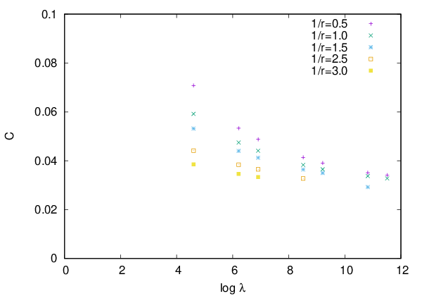
Figure 14: The coupling constant CC as a function of the momentum scale λ\lambda for a fixed value of 1/r=P2/m21/r=P^{2}/m^{2}, which is required for the scaling relation to hold. The plots from top to bottom correspond to 1/r=P2/m2=0.5,1.0,1.5,2.5,3.01/r=P^{2}/m^{2}=0.5,1.0,1.5,2.5,3.0.

Fig. 14 is the plot of the coupling constant CC as a function of the momentum scale λ\lambda for various but fixed values of 1/r:=P2/m21/r:=P^{2}/m^{2}, which is required for the scaling relation represented by Fig. 13 to hold. This is the renormalization group flow which gives the same physics, P/m=const.P/m=\text{const.}, namely, the same bound state mass for a given gluon mass mm. This result will be valid for relatively large λ\lambda due to the approximations adopted in this paper. As the cutoff λ\lambda increases, the coupling CC decreases like 1/ln⁡λ1/\ln\lambda and finally vanishes as λ→∞\lambda\to\infty:

C≅Const.ln⁡λ.\displaystyle C\cong\frac{\rm{Const.}}{\ln\lambda}. (106)

This behavior is consistent with the (ultraviolet) asymptotic freedom expected to hold in the Yang-Mills theory.
Refer to caption
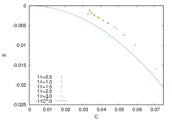
Figure 15: The plot of the β\beta function β⁡(C):=λ​d​Cd​λ\beta(C):=\lambda\frac{dC}{d\lambda} obtained from the numerical solutions of the BS equation (79a) for various values of P/mP/m: P2/m2=0.5,1.0,1.5,2.5,3.0P^{2}/m^{2}=0.5,1.0,1.5,2.5,3.0. The solid line denotes the β\beta function β⁡(C)=−113​C2\beta(C)=-\frac{11}{3}C^{2} obtained from the perturbation theory to one loop.

Fig. 15 shows the plot of the β\beta function β⁡(C):=λ​d​Cd​λ\beta(C):=\lambda\frac{dC}{d\lambda} calculated from the running of the coupling CC with respect to λ\lambda (Fig. 14) for various values of P/mP/m. We find that all the β\beta functions are negative and coincide for small CC or large λ\lambda independently of P/mP/m. The resulting β\beta function can be compared with the beta function β⁡(C)=−113​C2\beta(C)=-\frac{11}{3}C^{2} obtained by one-loop calculation in perturbation theory, which is indicated by the solid curve in Fig. 15. We find that all the points are well fitted to the single curve, although they are located slightly above the solid curve. We observe that the β\beta function obtained from the numerical solution of the BS equation has the same sign and order as the one-loop β\beta function. It should be remarked that the exact agreement of our result with the one loop prediction is not anticipated, since we have neglected some terms already in obtaining the kernel (79a). Our results indicate that the bound state solution of the BS equation is consistent with the asymptotic freedom in the Yang-Mills theory. This is one of the main results of this paper.

Finally, we give a comment how the derivative of CC with respect to λ\lambda is calculated numerically. The derivative was obtained by taking the finite difference between the smallest eigenvalues of CC at λ\lambda and 1.1​λ1.1\lambda for any fixed value of r−1=P2/m2r^{-1}=P^{2}/m^{2}. This approximation for the derivative becomes worse for larger λ\lambda. In view of this, we have used the data for the cutoff λ=105\lambda=10^{5} which is the largest possible value we can take due to the limitation of the computer memory available to us.

8 Conclusion and discussion

We summarize the results obtained in this paper. First, we have given a systematic derivation of the BS equation for the gluon and ghost BS amplitude by starting from the CJT effective action for the massive Yang-Mills theory. The solutions of the BS equation represent the simultaneous bound states for gluons and ghosts.

Second, we have obtained the numerical solutions of the derived BS equation in the ladder approximation with the standing gauge coupling, and the improved ladder approximation with the running gauge coupling. As a warming up problem, we restricted to the vanishing total momentum Pμ=0P^{\mu}=0. The we have found that (i) the gluon–gluon contribution is dominant in the solution, (ii) the ghost BS amplitude is much smaller than (at most 10% of) the gluon BS amplitude, (iii) the infrared behavior is influenced by the effect of the running coupling constant.

Third, armed with these preliminary investigations, we proceeded to obtain an approximate solution for the gluon-gluon BS amplitude alone, which corresponds to a two-gluon bound state as a candidate for a color singlet scalar glueball. We have calculated the beta functions through the running of the coupling constant by using the numerical solutions of the BS equation with an approximated kernel for different choices of the parameters, the ultraviolet cutoff and the constituent gluon mass. We have shown that the numerical results converge to a single function which has the same sign and order of magnitude as the one-loop beta function, although the exact agreement with the one-loop perturbation theory is not reproduced due to the approximation we adopted in obtaining the kernel of the BS equation. Thus, we have shown that the solution for the gluon bound state obtained in our approximation for the BS equation is consistent with the (ultraviolet) asymptotic freedom of the Yang-Mills theory.

It is obvious that we have a number of unsolved problems to be tackled: improvement of the kernel for the BS equation by incorporating more terms, examination of the high-energy behavior for performing the normalization of the BS amplitude, renormalization of the BS equation, improvement of the approximation to keep gauge invariance, e.g., through the Ward-Takahashi relations, confirmation of physical unitarity of the massive Yang-Mills theory, and so on. We hope to report some of the results in the near future.

Acknowledgment

This work is supported by Grants-in-Aid for Scientific Research (C) No.24540252 and (C) No.15K05042 from the Japan Society for the Promotion of Science (JSPS).

Appendix A BS kernel with a gauge parameter

We decompose the gluon propagator into the transverse part tμ​νt_{\mu\nu} and the longitudinal part ℓμ​ν\ell_{\mu\nu}:

Dμ​ν(0)​a​b​(k)\displaystyle D_{\mu\nu}^{(0)ab}(k) =−i​δa​bk2​(gμ​ν−kμ​kνk2)+−i​δa​bk2​α​kμ​kνk2\displaystyle=\frac{-i\delta^{ab}}{k^{2}}\left(g_{\mu\nu}-\frac{k_{\mu}k_{\nu}}{k^{2}}\right)+\frac{-i\delta^{ab}}{k^{2}}\alpha\frac{k_{\mu}k_{\nu}}{k^{2}}
:=−i​δa​bk2​[tμ​ν​(k)+α​ℓμ​ν​(k)].\displaystyle:=\frac{-i\delta^{ab}}{k^{2}}\left[t_{\mu\nu}(k)+\alpha\ell_{\mu\nu}(k)\right]. (107)

Here tμ​ν​(k)t_{\mu\nu}(k) and ℓμ​ν​(k)\ell_{\mu\nu}(k) satisfy the properties:

kμ​tμ​ν​(k)=0,kμ​ℓμ​ν​(k)=kν.\displaystyle k_{\mu}t_{\mu\nu}(k)=0,\quad k_{\mu}\ell_{\mu\nu}(k)=k_{\nu}. (108)

In order to simplify the expression, we use the identities:

p±=k−+q±=k+−q∓,q±=−k−+p±=k+−p∓.\displaystyle p^{\pm}=k^{-}+q^{\pm}=k^{+}-q^{\mp},\quad q^{\pm}=-k^{-}+p^{\pm}=k^{+}-p^{\mp}. (109)

The approximate kernel 𝒦(0)\mathcal{K}^{(0)} used in this paper is obtained from 𝒦\mathcal{K} of Fig. 7 by replacing the full propagators by the bare ones and neglecting the loop diagrams in KK.

The ghost-ghost kernel is given by

𝒦(0)​a​b;c​d\displaystyle\mathcal{K}^{(0)ab;cd} =−Γλ(0)​e​c​a​(k−,q+,p+)​Dλ​β(0)​e​e​(k−)​Γβ(0)​e​b​d​(−k−,p−,q−)​Δ(0)​c​c​(q+)​Δ(0)​d​d​(q−)\displaystyle=-\Gamma^{(0)eca}_{\lambda}(k^{-},q^{+},p^{+})D^{(0)ee}_{\lambda\beta}(k^{-})\Gamma^{(0)ebd}_{\beta}(-k^{-},p^{-},q^{-})\Delta^{(0)cc}(q^{+})\Delta^{(0)dd}(q^{-})
=−i​g2​fe​a​c​fe​b​d(k−)2​(q−)2​(q+)2​{pλ+​tλ​β​(k−)​pβ−+qλ+​α​ℓλ​β​(k−)​pβ−}.\displaystyle=-ig^{2}\frac{f^{eac}f^{ebd}}{(k^{-})^{2}(q^{-})^{2}(q^{+})^{2}}\left\{p_{\lambda}^{+}t_{\lambda\beta}(k^{-})p_{\beta}^{-}+q_{\lambda}^{+}\alpha\ell_{\lambda\beta}(k^{-})p_{\beta}^{-}\right\}. (110)

The ghost-gluon kernel is given by

𝒦(0)a​b;c​d;μ′ν′\displaystyle\mathcal{K}^{(0)}{}^{ab;cd}_{\ \ ;\mu^{\prime}\nu^{\prime}}
=\displaystyle= −(Γλ(0)​c​e​a​(q+,k−,p+)​Δ(0)​e​e​(k−)​Γβ(0)​d​b​e​(−q−,p−,k−)​Dλ​μ′(0)​c​c​(q+)​Dβ​ν′(0)​d​d​(q−)CLOSE\displaystyle-\Big(\Gamma^{(0)cea}_{\lambda}(q^{+},k^{-},p^{+})\Delta^{(0)ee}(k^{-})\Gamma^{(0)dbe}_{\beta}(-q^{-},p^{-},k^{-})D^{(0)cc}_{\lambda\mu^{\prime}}(q^{+})D^{(0)dd}_{\beta\nu^{\prime}}(q^{-})
OPEN+Γλ(0)​d​e​a​(−q−,k+,p+)​Δ(0)​e​e​(k+)​Γβ(0)​c​b​e​(q+,p−,k+)​Dβ​μ′(0)​c​c​(q+)​Dλ​ν′(0)​d​d​(q−))\displaystyle\hskip 28.45274pt+\Gamma^{(0)dea}_{\lambda}(-q^{-},k^{+},p^{+})\Delta^{(0)ee}(k^{+})\Gamma^{(0)cbe}_{\beta}(q^{+},p^{-},k^{+})D^{(0)cc}_{\beta\mu^{\prime}}(q^{+})D^{(0)dd}_{\lambda\nu^{\prime}}(q^{-})\Big)
=\displaystyle= −i​g2​fe​a​c​fe​b​d(k−)2​(q−)2​(q+)2​{pλ+​tλ​μ′​(q+)−α​qμ′++pλ+​α​ℓλ​μ′​(q+)}​{pβ−​tβ​ν′​(q−)+pβ−​α​ℓβ​ν′​(q−)}\displaystyle-ig^{2}\frac{f^{eac}f^{ebd}}{(k^{-})^{2}(q^{-})^{2}(q^{+})^{2}}\left\{p_{\lambda}^{+}t_{\lambda\mu^{\prime}}(q^{+})-\alpha q_{\mu^{\prime}}^{+}+p_{\lambda}^{+}\alpha\ell_{\lambda\mu^{\prime}}(q^{+})\right\}\left\{p_{\beta}^{-}t_{\beta\nu^{\prime}}(q^{-})+p^{-}_{\beta}\alpha\ell_{\beta\nu^{\prime}}(q^{-})\right\}
−i​g2​fe​a​d​fe​b​c(k+)2​(q−)2​(q+)2​{pλ+​tλ​ν′​(q−)+α​qν′−+pλ+​α​ℓλ​ν′​(q−)}​{pβ−​tβ​μ′​(q+)+pβ−​α​ℓβ​μ′​(q+)}.\displaystyle-ig^{2}\frac{f^{ead}f^{ebc}}{(k^{+})^{2}(q^{-})^{2}(q^{+})^{2}}\left\{p_{\lambda}^{+}t_{\lambda\nu^{\prime}}(q^{-})+\alpha q^{-}_{\nu^{\prime}}+p^{+}_{\lambda}\alpha\ell_{\lambda\nu^{\prime}}(q^{-})\right\}\left\{p_{\beta}^{-}t_{\beta\mu^{\prime}}(q^{+})+p^{-}_{\beta}\alpha\ell_{\beta\mu^{\prime}}(q^{+})\right\}. (111)

The gluon-ghost kernel is given by

𝒦(0)a​b;c​dμ​ν;=\displaystyle\mathcal{K}^{(0)}{}^{ab;cd}_{\mu\nu;}= −[Γμ(0)​a​c​e(−p+,q+,−k−)Δ(0)​e​e(−k−)Γν(0)​b​e​d(p−,−k−,q−)Δ(0)​c​c(q+)Δ(0)​d​d(q−)\displaystyle-\Big[\Gamma^{(0)ace}_{\mu}(-p^{+},q^{+},-k-)\Delta^{(0)ee}(-k^{-})\Gamma^{(0)bed}_{\nu}(p^{-},-k^{-},q^{-})\Delta^{(0)cc}(q^{+})\Delta^{(0)dd}(q^{-})
+Γμ(0)​a​e​d(−p+,k+,q−)Δ(0)​e​e(k+)Γν(0)​b​c​e(p−,q+,k+)Δ(0)​c​c(q+)Δ(0)​d​d(q−)]\displaystyle\hskip 28.45274pt+\Gamma^{(0)aed}_{\mu}(-p^{+},k^{+},q^{-})\Delta^{(0)ee}(k^{+})\Gamma^{(0)bce}_{\nu}(p^{-},q^{+},k^{+})\Delta^{(0)cc}(q^{+})\Delta^{(0)dd}(q^{-})\Big]
=\displaystyle= i​g2​fe​a​c​fe​b​d(k−)2​(q−)2​(q+)2​qμ+​kν−−i​g2​fe​a​d​fe​b​c(k+)2​(q−)2​(q+)2​kμ+​qν+.\displaystyle ig^{2}\frac{f^{eac}f^{ebd}}{(k^{-})^{2}(q^{-})^{2}(q^{+})^{2}}q^{+}_{\mu}k^{-}_{\nu}-ig^{2}\frac{f^{ead}f^{ebc}}{(k^{+})^{2}(q^{-})^{2}(q^{+})^{2}}k^{+}_{\mu}q^{+}_{\nu}. (112)

The gluon-ghost kernel 𝒦(0)​c​d;a​b;μν\mathcal{K}^{(0)cd;ab}_{\ \ ;\mu\nu} does not have the gauge parameter dependence, since the external gluon propagator does not contribute to the kernel and there does not exist ghosts in the internal lines.

The gluon-gluon kernel 𝒦μ​ν;μ′​ν′(0)​a​b;c​d\mathcal{K}^{(0)ab;cd}_{\ \ \,\mu\nu;\mu^{\prime}\nu^{\prime}} consists of three parts.

𝒦(0)a​b;c​dμ​ν;μ′​ν′=K3Gla​b;c​dμ​ν;μ′​ν′+K3Glcrossa​b;c​dμ​ν;μ′​ν′+K4Gla​b;c​dμ​ν;μ′​ν′,\displaystyle\mathcal{K}^{(0)}{}^{ab;cd}_{\mu\nu;\mu^{\prime}\nu^{\prime}}=K_{\text{3Gl}}{}^{ab;cd}_{\mu\nu;\mu^{\prime}\nu^{\prime}}+K_{\text{3Gl}}^{\text{cross}}{}^{ab;cd}_{\mu\nu;\mu^{\prime}\nu^{\prime}}+K_{\text{4Gl}}{}^{ab;cd}_{\mu\nu;\mu^{\prime}\nu^{\prime}}, (113a)
K3Gla​b;c​dμ​ν;μ′​ν′\displaystyle K_{\text{3Gl}}{}^{ab;cd}_{\mu\nu;\mu^{\prime}\nu^{\prime}} =Γμ​γ​λ(0)​a​c​e​(−p+,q+,k−)​Dλ​λ′(0)​e​e​(k−)​Γν​γ′​λ′(0)​b​d​e​(p−,−q−,−k−)​Dγ​μ′(0)​c​c​(q+)​Dγ′​ν′(0)​d​d​(q−)\displaystyle=\Gamma^{(0)ace}_{\mu\gamma\lambda}(-p^{+},q^{+},k^{-})D^{(0)ee}_{\lambda\lambda^{\prime}}(k^{-})\Gamma^{(0)bde}_{\nu\gamma^{\prime}\lambda^{\prime}}(p^{-},-q^{-},-k^{-})D^{(0)cc}_{\gamma\mu^{\prime}}(q^{+})D^{(0)dd}_{\gamma^{\prime}\nu^{\prime}}(q^{-})
=i​g2​fe​a​c​fe​b​d(k−)2​(q−)2​(q+)2​[tλ​λ′​(k−)+α​ℓλ​λ′​(k−)]​[tγ′​ν′​(q−)+α​ℓγ′​ν′​(q−)]\displaystyle=ig^{2}\frac{f^{eac}f^{ebd}}{(k^{-})^{2}(q^{-})^{2}(q^{+})^{2}}\left[t_{\lambda\lambda^{\prime}}(k^{-})+\alpha\ell_{\lambda\lambda^{\prime}}(k^{-})\right]\left[t_{\gamma^{\prime}\nu^{\prime}}(q^{-})+\alpha\ell_{\gamma^{\prime}\nu^{\prime}}(q^{-})\right]
×[tγ​μ′​(q+)+α​ℓγ​μ′​(q+)]​[(qγ+−2​pγ+)​gλ​μ+(2​pλ+−kλ−)​gγ​μ+(pμ+−2​qμ+)​gλ​γ]\displaystyle\hskip 0.0pt\times\left[t_{\gamma\mu^{\prime}}(q^{+})+\alpha\ell_{\gamma\mu^{\prime}}(q^{+})\right]\left[(q^{+}_{\gamma}-2p^{+}_{\gamma})g_{\lambda\mu}+(2p^{+}_{\lambda}-k^{-}_{\lambda})g_{\gamma\mu}+(p^{+}_{\mu}-2q^{+}_{\mu})g_{\lambda\gamma}\right]
×[(2​pλ′−−kλ′−)​gν​γ′+(qγ′−−2​pγ′−)​gν​λ′+(pν−−2​qν−)​gλ′​γ′],\displaystyle\hskip 0.0pt\times\left[(2p^{-}_{\lambda^{\prime}}-k^{-}_{\lambda^{\prime}})g_{\nu\gamma^{\prime}}+(q^{-}_{\gamma^{\prime}}-2p^{-}_{\gamma^{\prime}})g_{\nu\lambda^{\prime}}+(p^{-}_{\nu}-2q^{-}_{\nu})g_{\lambda^{\prime}\gamma^{\prime}}\right], (113b)
K3Glcrossa​b;c​dμ​ν;μ′​ν′=\displaystyle K_{\text{3Gl}}^{\text{cross}}{}^{ab;cd}_{\mu\nu;\mu^{\prime}\nu^{\prime}}= Γμ​γ​λ(0)​a​d​e​(−p+,−q−,k+)​Dλ′​λ(0)​e​e​(k+)​Γν​γ′​λ′(0)​b​c​e​(p−,q+,−k+)​Dγ′​μ′(0)​c​c​(q+)​Dγ​ν′(0)​d​d​(q−)\displaystyle\Gamma^{(0)ade}_{\mu\gamma\lambda}(-p^{+},-q^{-},k^{+})D^{(0)ee}_{\lambda^{\prime}\lambda}(k^{+})\Gamma^{(0)bce}_{\nu\gamma^{\prime}\lambda^{\prime}}(p^{-},q^{+},-k^{+})D^{(0)cc}_{\gamma^{\prime}\mu^{\prime}}(q^{+})D^{(0)dd}_{\gamma\nu^{\prime}}(q^{-})
=\displaystyle= i​g2​fe​a​d​fe​b​c(k+)2​(q−)2​(q+)2​[tλ​λ′​(k+)+α​ℓλ​λ′​(k+)]​[tγ​ν′​(q−)+α​ℓγ​ν′​(q−)]\displaystyle ig^{2}\frac{f^{ead}f^{ebc}}{(k^{+})^{2}(q^{-})^{2}(q^{+})^{2}}\left[t_{\lambda\lambda^{\prime}}(k^{+})+\alpha\ell_{\lambda\lambda^{\prime}}(k^{+})\right]\left[t_{\gamma\nu^{\prime}}(q^{-})+\alpha\ell_{\gamma\nu^{\prime}}(q^{-})\right]
×[tγ′​μ′​(q+)+α​ℓγ′​μ′​(q+)]​[(2​pλ+−kλ+)​gγ​μ−(2​pγ++qγ−)​gλ​μ+(pμ++2​qμ−)​gλ​γ]\displaystyle\hskip 0.0pt\times\left[t_{\gamma^{\prime}\mu^{\prime}}(q^{+})+\alpha\ell_{\gamma^{\prime}\mu^{\prime}}(q^{+})\right]\left[(2p^{+}_{\lambda}-k^{+}_{\lambda})g_{\gamma\mu}-(2p^{+}_{\gamma}+q^{-}_{\gamma})g_{\lambda\mu}+(p^{+}_{\mu}+2q^{-}_{\mu})g_{\lambda\gamma}\right]
×[(2​pλ′−−kλ′+)​gν​γ′−(2​pγ′−+qγ′+)​gν​λ′+(pν−+2​qν+)​gλ′​γ′],\displaystyle\hskip 0.0pt\times\left[(2p^{-}_{\lambda^{\prime}}-k^{+}_{\lambda^{\prime}})g_{\nu\gamma^{\prime}}-(2p^{-}_{\gamma^{\prime}}+q^{+}_{\gamma^{\prime}})g_{\nu\lambda^{\prime}}+(p^{-}_{\nu}+2q^{+}_{\nu})g_{\lambda^{\prime}\gamma^{\prime}}\right], (113c)
K4Gla​b;c​dμ​ν;μ′​ν′\displaystyle K_{\text{4Gl}}{}^{ab;cd}_{\mu\nu;\mu^{\prime}\nu^{\prime}} =Γμ​ν​γ​δ(0)​a​b​d​c​(−p+,p−,−q−,q+)​Dδ​μ′(0)​c​c​(q+)​Dγ​ν′(0)​d​d​(q−)\displaystyle=\Gamma^{(0)abdc}_{\mu\nu\gamma\delta}(-p^{+},p^{-},-q^{-},q^{+})D^{(0)cc}_{\delta\mu^{\prime}}(q^{+})D^{(0)dd}_{\gamma\nu^{\prime}}(q^{-})
=g2(q−)2​(a+)2​[tγ​ν′​(q−)+α​ℓγ​ν′​(q−)]​[tδ​μ​(q+)+α​ℓδ​μ​(q+)]\displaystyle=\frac{g^{2}}{(q^{-})^{2}(a^{+})^{2}}\left[t_{\gamma\nu^{\prime}}(q^{-})+\alpha\ell_{\gamma\nu^{\prime}}(q^{-})\right]\left[t_{\delta\mu}(q^{+})+\alpha\ell_{\delta\mu}(q^{+})\right]
×[fe​a​dfe​b​c(gγ​δgμ​ν−gγ​νgδ​μ)+fe​a​cfe​b​d(gγ​δgμ​ν−gγ​μgδ​ν)\displaystyle\hskip 0.0pt\times[f^{ead}f^{ebc}\left(g_{\gamma\delta}g_{\mu\nu}-g_{\gamma\nu}g_{\delta\mu}\right)+f^{eac}f^{ebd}\left(g_{\gamma\delta}g_{\mu\nu}-g_{\gamma\mu}g_{\delta\nu}\right)
−fe​a​bfe​c​d(gγ​μgδ​ν−gγ​νgδ​μ)].\displaystyle-f^{eab}f^{ecd}\left(g_{\gamma\mu}g_{\delta\nu}-g_{\gamma\nu}g_{\delta\mu}\right)]. (113d)

Appendix B BS Kernel in the Landau gauge

B.1 Pμ≠0P^{\mu}\not=0

In the Landau gauge (α=0\alpha=0), the kernels given in the above take the simpler forms:

𝒦(0)​a​b;c​d=\displaystyle\mathcal{K}^{(0)ab;cd}= −i​g2​fe​a​c​fe​b​d(k−)2​(q−)2​(q+)2​(p+⋅p−+(p+⋅k−)​(k−⋅p−)(k−)2),\displaystyle-ig^{2}\frac{f^{eac}f^{ebd}}{(k^{-})^{2}(q^{-})^{2}(q^{+})^{2}}\left(p^{+}\cdot p^{-}+\frac{(p^{+}\cdot k^{-})(k^{-}\cdot p^{-})}{(k^{-})^{2}}\right), (114)
𝒦(0)​a​b;c​d;μ′ν′=\displaystyle\mathcal{K}^{(0)ab;cd}_{\ \ \ \ \ ;\mu^{\prime}\nu^{\prime}}= −i​g2​fe​a​c​fe​b​d(k−)2​(q−)2​(q+)2​(pμ′+−qμ′+​p+⋅q+(q+)2)​(pν′−−qν′−​p−⋅q−(q−)2)\displaystyle-ig^{2}\frac{f^{eac}f^{ebd}}{(k^{-})^{2}(q^{-})^{2}(q^{+})^{2}}\left(p^{+}_{\mu^{\prime}}-q^{+}_{\mu^{\prime}}\frac{p^{+}\cdot q^{+}}{(q^{+})^{2}}\right)\left(p^{-}_{\nu^{\prime}}-q^{-}_{\nu^{\prime}}\frac{p^{-}\cdot q^{-}}{(q^{-})^{2}}\right)
−i​g2​fe​a​d​fe​b​c(k+)2​(q−)2​(q+)2​(pμ′−−qμ′+​p−⋅q+(q+)2)​(pν′+−qν′−​p+⋅q−(q−)2),\displaystyle-ig^{2}\frac{f^{ead}f^{ebc}}{(k^{+})^{2}(q^{-})^{2}(q^{+})^{2}}\left(p^{-}_{\mu^{\prime}}-q^{+}_{\mu^{\prime}}\frac{p^{-}\cdot q^{+}}{(q^{+})^{2}}\right)\left(p^{+}_{\nu^{\prime}}-q^{-}_{\nu^{\prime}}\frac{p^{+}\cdot q^{-}}{(q^{-})^{2}}\right), (115)
𝒦μ​ν;(0)​a​b;c​d=\displaystyle\mathcal{K}^{(0)ab;cd}_{\ \ \,\mu\nu;}= i​g2​fe​a​c​fe​b​d(k−)2​(q−)2​(q+)2​qμ+​kν−−i​g2​fe​a​d​fe​b​c(k+)2​(q−)2​(q+)2​kμ+​qν+,\displaystyle ig^{2}\frac{f^{eac}f^{ebd}}{(k^{-})^{2}(q^{-})^{2}(q^{+})^{2}}q^{+}_{\mu}k^{-}_{\nu}-ig^{2}\frac{f^{ead}f^{ebc}}{(k^{+})^{2}(q^{-})^{2}(q^{+})^{2}}k^{+}_{\mu}q^{+}_{\nu}, (116)
𝒦μ​ν;μ′​ν′(0)​a​b;c​d=\displaystyle\mathcal{K}^{(0)ab;cd}_{\ \ \,\mu\nu;\mu^{\prime}\nu^{\prime}}= i​g2​fe​a​c​fe​b​d(k−)2​(q−)2​(q+)2\displaystyle ig^{2}\frac{f^{eac}f^{ebd}}{(k^{-})^{2}(q^{-})^{2}(q^{+})^{2}}
×[−4pλ′−tμ​λ′(k−)tν​ν′(q−)tγ​μ′(q+)pγ++4pλ+tλ​λ′(k−)pλ′−tν​ν′(q−)tμ​μ′(q+)\displaystyle\hskip 0.0pt\times\Big[-4p^{-}_{\lambda^{\prime}}t_{\mu\lambda^{\prime}}(k^{-})t_{\nu\nu^{\prime}}(q^{-})t_{\gamma\mu^{\prime}}(q^{+})p^{+}_{\gamma}+4p^{+}_{\lambda}t_{\lambda\lambda^{\prime}}(k^{-})p^{-}_{\lambda^{\prime}}t_{\nu\nu^{\prime}}(q^{-})t_{\mu\mu^{\prime}}(q^{+})
+2​pμ+​tγ​λ′​(k−)​pλ′−​tν​ν′​(q−)​tγ​μ′​(q+)+4​tμ​ν​(k−)​pγ′−​tγ′​ν′​(q−)​tγ​μ′​(q+)​pγ+\displaystyle\hskip 14.22636pt+2p^{+}_{\mu}t_{\gamma\lambda^{\prime}}(k^{-})p^{-}_{\lambda^{\prime}}t_{\nu\nu^{\prime}}(q^{-})t_{\gamma\mu^{\prime}}(q^{+})+4t_{\mu\nu}(k^{-})p^{-}_{\gamma^{\prime}}t_{\gamma^{\prime}\nu^{\prime}}(q^{-})t_{\gamma\mu^{\prime}}(q^{+})p^{+}_{\gamma}
−4​pλ+​tλ​ν​(k−)​pγ′−​tγ′​ν′​(q−)​tμ​μ′​(q+)−2​pμ+​tγ​ν​(k−)​pγ′−​tγ′​ν′​(q−)​tγ​μ′​(q+)\displaystyle\hskip 14.22636pt-4p^{+}_{\lambda}t_{\lambda\nu}(k^{-})p^{-}_{\gamma^{\prime}}t_{\gamma^{\prime}\nu^{\prime}}(q^{-})t_{\mu\mu^{\prime}}(q^{+})-2p^{+}_{\mu}t_{\gamma\nu}(k^{-})p^{-}_{\gamma^{\prime}}t_{\gamma^{\prime}\nu^{\prime}}(q^{-})t_{\gamma\mu^{\prime}}(q^{+})
+(pν−−2qν−){−2tμ​λ′(k−)tλ′​ν′(q−)tγ​μ′(q+)pγ+\displaystyle\hskip 14.22636pt+(p^{-}_{\nu}-2q^{-}_{\nu})\big\{-2t_{\mu\lambda^{\prime}}(k^{-})t_{\lambda^{\prime}\nu^{\prime}}(q^{-})t_{\gamma\mu^{\prime}}(q^{+})p^{+}_{\gamma}
+2pλ+tλ​λ′(k−)tλ′​ν′(q−)tμ​μ′(q+)+pμ+tγ​λ′(k−)tλ′​ν′(q−)tγ​μ′(q+)}]\displaystyle\hskip 14.22636pt+2p^{+}_{\lambda}t_{\lambda\lambda^{\prime}}(k^{-})t_{\lambda^{\prime}\nu^{\prime}}(q^{-})t_{\mu\mu^{\prime}}(q^{+})+p^{+}_{\mu}t_{\gamma\lambda^{\prime}}(k^{-})t_{\lambda^{\prime}\nu^{\prime}}(q^{-})t_{\gamma\mu^{\prime}}(q^{+})\big\}\Big]
+i​g2​fe​a​c​fe​b​d(k+)2​(q−)2​(q+)2\displaystyle+ig^{2}\frac{f^{eac}f^{ebd}}{(k^{+})^{2}(q^{-})^{2}(q^{+})^{2}}
×[4pλ+tλ​λ′(k+)pλ′−tμ​ν′(q−)tν​μ′(q+)−4tμ​λ′(k+)pλ′−pγ+tγ​ν′(q−)tν​μ′(q+)\displaystyle\hskip 0.0pt\times\Big[4p^{+}_{\lambda}t_{\lambda\lambda^{\prime}}(k^{+})p^{-}_{\lambda^{\prime}}t_{\mu\nu^{\prime}}(q^{-})t_{\nu\mu^{\prime}}(q^{+})-4t_{\mu\lambda^{\prime}}(k^{+})p^{-}_{\lambda^{\prime}}p^{+}_{\gamma}t_{\gamma\nu^{\prime}}(q^{-})t_{\nu\mu^{\prime}}(q^{+})
+2​(pμ++2​qμ−)​pλ′−​tλ​λ′​(k+)​tλ​ν′​(q−)​tν​μ′​(q+)−4​pλ+​tλ​ν​(k+)​tμ​ν′​(q−)​tγ′​μ′​(q+)​pγ′−\displaystyle\hskip 14.22636pt+2(p^{+}_{\mu}+2q^{-}_{\mu})p^{-}_{\lambda^{\prime}}t_{\lambda\lambda^{\prime}}(k^{+})t_{\lambda\nu^{\prime}}(q^{-})t_{\nu\mu^{\prime}}(q^{+})-4p^{+}_{\lambda}t_{\lambda\nu}(k^{+})t_{\mu\nu^{\prime}}(q^{-})t_{\gamma^{\prime}\mu^{\prime}}(q^{+})p^{-}_{\gamma^{\prime}}
+4​tμ​ν​(k+)​pγ+​tγ​ν′​(q−)​pγ′−​tγ′​μ′​(q+)−2​(pμ++2​qμ−)​tλ​ν​(k+)​tλ​ν′​(q−)​pγ′−​tγ′​μ′​(q+)\displaystyle\hskip 14.22636pt+4t_{\mu\nu}(k^{+})p^{+}_{\gamma}t_{\gamma\nu^{\prime}}(q^{-})p^{-}_{\gamma^{\prime}}t_{\gamma^{\prime}\mu^{\prime}}(q^{+})-2(p^{+}_{\mu}+2q^{-}_{\mu})t_{\lambda\nu}(k^{+})t_{\lambda\nu^{\prime}}(q^{-})p^{-}_{\gamma^{\prime}}t_{\gamma^{\prime}\mu^{\prime}}(q^{+})
+(pν−+2qν+){2pλ+tλ​λ′(k+)tμ​ν′(q−)tλ′​μ′(q+)−2tμ​λ′(k+)pγ+tγ​ν′(q−)tλ′​μ′(q+)\displaystyle\hskip 14.22636pt+(p^{-}_{\nu}+2q^{+}_{\nu})\big\{2p^{+}_{\lambda}t_{\lambda\lambda^{\prime}}(k^{+})t_{\mu\nu^{\prime}}(q^{-})t_{\lambda^{\prime}\mu^{\prime}}(q^{+})-2t_{\mu\lambda^{\prime}}(k^{+})p^{+}_{\gamma}t_{\gamma\nu^{\prime}}(q^{-})t_{\lambda^{\prime}\mu^{\prime}}(q^{+})
+(pμ++2qμ−)tλ​λ′(k+)tλ​ν′(q−)tλ′​μ′(q+)}]\displaystyle\hskip 14.22636pt+(p^{+}_{\mu}+2q^{-}_{\mu})t_{\lambda\lambda^{\prime}}(k^{+})t_{\lambda\nu^{\prime}}(q^{-})t_{\lambda^{\prime}\mu^{\prime}}(q^{+})\big\}\Big]
−ig21(q−)2​(q+)2[fe​a​dfe​b​c(tγ​ν′(q−)tγ​μ′(q+)gμ​ν−tν​ν′(q−)tμ​μ′(q+))\displaystyle-ig^{2}\frac{1}{(q^{-})^{2}(q^{+})^{2}}\Big[f^{ead}f^{ebc}\left(t_{\gamma\nu^{\prime}}(q^{-})t_{\gamma\mu^{\prime}}(q^{+})g_{\mu\nu}-t_{\nu\nu^{\prime}}(q^{-})t_{\mu\mu^{\prime}}(q^{+})\right)
+fe​a​c​fe​b​d​(tγ​ν′​(q−)​tγ​μ′​(q+)​gμ​ν−tμ​ν′​(q−)​tν​μ′​(q+))\displaystyle\hskip 85.35826pt+f^{eac}f^{ebd}\left(t_{\gamma\nu^{\prime}}(q^{-})t_{\gamma\mu^{\prime}}(q^{+})g_{\mu\nu}-t_{\mu\nu^{\prime}}(q^{-})t_{\nu\mu^{\prime}}(q^{+})\right)
−fe​a​bfe​c​d(tμ​ν′(q−)tν​μ′(q+)−tν​ν′(q−)tμ​μ′(q+))].\displaystyle\hskip 85.35826pt-f^{eab}f^{ecd}\left(t_{\mu\nu^{\prime}}(q^{-})t_{\nu\mu^{\prime}}(q^{+})-t_{\nu\nu^{\prime}}(q^{-})t_{\mu\mu^{\prime}}(q^{+})\right)\Big]. (117)

B.2 Pμ=0P^{\mu}=0

We give the kernel in the simplest case Pμ=0P_{\mu}=0. The BS amplitudes obtained by solving the BS equation at Pμ=0P_{\mu}=0 from the beginning may agree with those obtained in the limit of Pμ=0P_{\mu}=0 of the solution of the BS equation with Pμ≠0P_{\mu}\not=0, if the vector model has the same property as the Wick–Cutkosky model which is the exactly solved model for the scalar particles. Notice that transversality changes at Pμ=0P_{\mu}=0. In the limit Pμ→0P_{\mu}\to 0, A2A_{2} is ill-defined. The ordinary transverse tensor is reproduced at Pμ=0P_{\mu}=0, since there is no difference between k+k^{+} and k−k^{-} at Pμ=0P_{\mu}=0 The BS equation cannot contain A2A_{2} part once Pμ=0P_{\mu}=0 is adopted:

(A1​(p)B⁡(p))=\displaystyle\begin{pmatrix}A_{1}(p)\\ B(p)\end{pmatrix}= −ig2∫d4​q(2​π)4fe​a​c​fe​a​d(p−q)2​q4(a11a12a21a22)(A1​(q)B⁡(q))\displaystyle-ig^{2}\int\frac{d^{4}q}{(2\pi)^{4}}\frac{f^{eac}f^{ead}}{(p-q)^{2}q^{4}}\begin{pmatrix}a_{11}&a_{12}\\ a_{21}&a_{22}\\ \end{pmatrix}\begin{pmatrix}A_{1}(q)\\ B(q)\end{pmatrix}
−ig2∫d4​q(2​π)4fe​a​c​fe​a​d(p+q)2​q4(b11b12b210)(A1​(q)B⁡(q)).\displaystyle-ig^{2}\int\frac{d^{4}q}{(2\pi)^{4}}\frac{f^{eac}f^{ead}}{(p+q)^{2}q^{4}}\begin{pmatrix}b_{11}&b_{12}\\ b_{21}&0\\ \end{pmatrix}\begin{pmatrix}A_{1}(q)\\ B(q)\end{pmatrix}. (118)

Here ai​ja_{ij} denotes the contribution from the non-crossing diagrams, while bi​jb_{ij} from the crossing diagrams. Therefore, b22=0b_{22}=0 is due to the fact that there do not exist the ghost crossing diagrams in the ghost-ghost kernel. The explicit form of the matrix elements are as follows.

a113Gl\displaystyle a_{11}^{\text{3Gl}} =14p4q2+p2(−38q2p⋅q−11(p⋅q)2+35q4)+4(−9q4p⋅q+q2(p⋅q)2+5(p⋅q)3+3q6)3​q2​(p−q)2,\displaystyle=\frac{14p^{4}q^{2}+p^{2}\left(-38q^{2}p\cdot q-11(p\cdot q)^{2}+35q^{4}\right)+4\left(-9q^{4}p\cdot q+q^{2}(p\cdot q)^{2}+5(p\cdot q)^{3}+3q^{6}\right)}{3q^{2}\left(p-q\right)^{2}},
a114Gl\displaystyle a_{11}^{\text{4Gl}} =−6​(p−q)2,\displaystyle=-6(p-q)^{2},
a12\displaystyle a_{12} =13​(p⋅q−q2),a21=−p2​q2−(p⋅q)22​q2,a22=−p2​q2−(p⋅q)2(p−q)2,\displaystyle=\frac{1}{3}\left(p\cdot q-q^{2}\right),\quad a_{21}=-\frac{p^{2}q^{2}-(p\cdot q)^{2}}{2q^{2}},\quad a_{22}=-\frac{p^{2}q^{2}-(p\cdot q)^{2}}{(p-q)^{2}},
b11\displaystyle b_{11} =14​p4​q2+p2​(38​q2​p⋅q−11​(p⋅q)2+35​q4)+4​(9​q4​p⋅q+q2​(p⋅q)2−5​(p⋅q)3+3​q6)3​q2​(p+q)2,\displaystyle=\frac{14p^{4}q^{2}+p^{2}\left(38q^{2}p\cdot q-11(p\cdot q)^{2}+35q^{4}\right)+4\left(9q^{4}p\cdot q+q^{2}(p\cdot q)^{2}-5(p\cdot q)^{3}+3q^{6}\right)}{3q^{2}\left(p+q\right)^{2}},
b12\displaystyle b_{12} =−13​(p⋅q+q2),b21=−p2​q2−(p⋅q)22​q2.\displaystyle=-\frac{1}{3}\left(p\cdot q+q^{2}\right),\quad b_{21}=-\frac{p^{2}q^{2}-(p\cdot q)^{2}}{2q^{2}}. (119)

We perform the Wick rotation to p,qp,q.

p0\displaystyle p_{0} =i​p4,p2=p02−p12−p22−p32=−(p12+p22+p32+p42):=−pE2.\displaystyle=ip_{4},\quad p^{2}=p_{0}^{2}-p_{1}^{2}-p_{2}^{2}-p_{3}^{2}=-(p_{1}^{2}+p_{2}^{2}+p_{3}^{2}+p_{4}^{2}):=-p_{E}^{2}. (120)

This is applied also to qq. In what follows, we omit the index EE. Consequently, we can perform the integration over the four-dimensional coordinates by converting it to the integration in the four-dimensional Euclidean space.

(A1​(p)B⁡(p))=\displaystyle\begin{pmatrix}A_{1}(p)\\ B(p)\end{pmatrix}= g2​∫q2​sin2⁡θ​d​q2​d​θ(2​π)3​fe​a​c​fe​a​d(p−q)2​q4​(a11a12a21a22)​(A1​(q)B⁡(q))\displaystyle g^{2}\int\frac{q^{2}\sin^{2}\theta dq^{2}d\theta}{(2\pi)^{3}}\frac{f^{eac}f^{ead}}{(p-q)^{2}q^{4}}\begin{pmatrix}a_{11}&a_{12}\\ a_{21}&a_{22}\\ \end{pmatrix}\begin{pmatrix}A_{1}(q)\\ B(q)\end{pmatrix}
+g2∫q2​sin2⁡θ​d​q2​d​θ(2​π)3fe​a​c​fe​a​d(p+q)2​q4(b11b12b210)(A1​(q)B⁡(q))\displaystyle+g^{2}\int\frac{q^{2}\sin^{2}\theta dq^{2}d\theta}{(2\pi)^{3}}\frac{f^{eac}f^{ead}}{(p+q)^{2}q^{4}}\begin{pmatrix}b_{11}&b_{12}\\ b_{21}&0\\ \end{pmatrix}\begin{pmatrix}A_{1}(q)\\ B(q)\end{pmatrix}
=\displaystyle= g2​fe​a​c​fe​a​d​∫d​q216​π2​2π​∫q2​sin2⁡θ​d​θ(p−q)2​q4​(a11a12a21a22)​(A1​(q)B⁡(q))\displaystyle g^{2}f^{eac}f^{ead}\int\frac{dq^{2}}{16\pi^{2}}\frac{2}{\pi}\int\frac{q^{2}\sin^{2}\theta d\theta}{(p-q)^{2}q^{4}}\begin{pmatrix}a_{11}&a_{12}\\ a_{21}&a_{22}\\ \end{pmatrix}\begin{pmatrix}A_{1}(q)\\ B(q)\end{pmatrix}
+g2fe​a​cfe​a​d∫d​q216​π22πq2​sin2⁡θ​d​θ(p+q)2​q4(b11b12b210)(A1​(q)B⁡(q)).\displaystyle+g^{2}f^{eac}f^{ead}\int\frac{dq^{2}}{16\pi^{2}}\frac{2}{\pi}\frac{q^{2}\sin^{2}\theta d\theta}{(p+q)^{2}q^{4}}\begin{pmatrix}b_{11}&b_{12}\\ b_{21}&0\\ \end{pmatrix}\begin{pmatrix}A_{1}(q)\\ B(q)\end{pmatrix}. (121)

Assuming that A1​(q)A_{1}(q) and B⁡(q)B(q) do not depend on the angles, we can perform the angular integration to obtain

(A1​(p2)B⁡(p2))=\displaystyle\begin{pmatrix}A_{1}(p^{2})\\ B(p^{2})\end{pmatrix}= g2​fe​a​c​fe​a​d​∫d​q216​π2​(a11a12a21a22)​(A1​(q2)B⁡(q2))\displaystyle g^{2}f^{eac}f^{ead}\int\frac{dq^{2}}{16\pi^{2}}\begin{pmatrix}a_{11}&a_{12}\\ a_{21}&a_{22}\\ \end{pmatrix}\begin{pmatrix}A_{1}(q^{2})\\ B(q^{2})\end{pmatrix}
+g2fe​a​cfe​a​d∫d​q216​π2(b11b12b210)(A1​(q2)B⁡(q2)),\displaystyle+g^{2}f^{eac}f^{ead}\int\frac{dq^{2}}{16\pi^{2}}\begin{pmatrix}b_{11}&b_{12}\\ b_{21}&0\\ \end{pmatrix}\begin{pmatrix}A_{1}(q^{2})\\ B(q^{2})\end{pmatrix}, (122)

where the matrix elements are given as

a11\displaystyle a_{11} =a113​G​l+a114​G​l\displaystyle=a_{11}^{3Gl}+a_{11}^{4Gl}
={(113​p2+154​q2)+(−6q2)}​θ​(p2−q2)+{(−7​p412​q6+4​p2q4+4q2)+(−6q2)}​θ​(q2−p2),\displaystyle=\left\{\left(\frac{11}{3p^{2}}+\frac{15}{4q^{2}}\right)+\left(-\frac{6}{q^{2}}\right)\right\}\theta(p^{2}-q^{2})+\left\{\left(-\frac{7p^{4}}{12q^{6}}+\frac{4p^{2}}{q^{4}}+\frac{4}{q^{2}}\right)+\left(-\frac{6}{q^{2}}\right)\right\}\theta(q^{2}-p^{2}),
a12\displaystyle a_{12} =−16​p2​θ​(p2−q2)+16​p2−2​q2q4​θ​(q2−p2),\displaystyle=-\frac{1}{6p^{2}}\theta(p^{2}-q^{2})+\frac{1}{6}\frac{p^{2}-2q^{2}}{q^{4}}\theta(q^{2}-p^{2}),
a21\displaystyle a_{21} =18​(1p2−3q2)​θ​(p2−q2)+p4−3​p2​q28​q6​θ​(q2−p2),\displaystyle=\frac{1}{8}\left(\frac{1}{p^{2}}-\frac{3}{q^{2}}\right)\theta(p^{2}-q^{2})+\frac{p^{4}-3p^{2}q^{2}}{8q^{6}}\theta(q^{2}-p^{2}),
a22\displaystyle a_{22} =(−34​p2)​θ​(p2−q2)+(−3​p24​q4)​θ​(q2−p2),\displaystyle=\left(-\frac{3}{4p^{2}}\right)\theta(p^{2}-q^{2})+\left(-\frac{3p^{2}}{4q^{4}}\right)\theta(q^{2}-p^{2}),
b11\displaystyle b_{11} =(113​p2+154​q2)​θ​(p2−q2)+(−7​p412​q6+4​p2q4+4q2)​θ​(q2−p2),\displaystyle=\left(\frac{11}{3p^{2}}+\frac{15}{4q^{2}}\right)\theta(p^{2}-q^{2})+\left(-\frac{7p^{4}}{12q^{6}}+\frac{4p^{2}}{q^{4}}+\frac{4}{q^{2}}\right)\theta(q^{2}-p^{2}),
b12\displaystyle b_{12} =(−16​p2)​θ​(p2−q2)+(p2−2​q26​q4)​θ​(q2−p2),\displaystyle=\left(-\frac{1}{6p^{2}}\right)\theta(p^{2}-q^{2})+\left(\frac{p^{2}-2q^{2}}{6q^{4}}\right)\theta(q^{2}-p^{2}),
b21\displaystyle b_{21} =18​(1p2−3q2)​θ​(p2−q2)+p4−3​p2​q28​q6​θ​(q2−p2).\displaystyle=\frac{1}{8}\left(\frac{1}{p^{2}}-\frac{3}{q^{2}}\right)\theta(p^{2}-q^{2})+\frac{p^{4}-3p^{2}q^{2}}{8q^{6}}\theta(q^{2}-p^{2}). (123)

Here we have used the formulae for the angular integrations which are given e.g., in [13]. We find that the non-crossing and crossing diagrams give the same contributions to the kernel. This is consistent with the assumption that A1A_{1} and BB depend only on the magnitude of the Euclidean momentum.

(A1​(p2)B⁡(p2))=C​∫d​q2​(a~11a~12a~21a~22)​(A1​(q2)B⁡(q2)),\begin{pmatrix}A_{1}(p^{2})\\ B(p^{2})\end{pmatrix}=C\int dq^{2}\begin{pmatrix}\tilde{a}_{11}&\tilde{a}_{12}\\ \tilde{a}_{21}&\tilde{a}_{22}\\ \end{pmatrix}\begin{pmatrix}A_{1}(q^{2})\\ B(q^{2})\end{pmatrix}, (124)

with

a~11\displaystyle\tilde{a}_{11} ={223​p2+32​q2}​θ​(p2−q2)+{−7​p46​q6+8​p2q4+2q2}​θ​(q2−p2),\displaystyle=\left\{\frac{22}{3p^{2}}+\frac{3}{2q^{2}}\right\}\theta(p^{2}-q^{2})+\left\{-\frac{7p^{4}}{6q^{6}}+\frac{8p^{2}}{q^{4}}+\frac{2}{q^{2}}\right\}\theta(q^{2}-p^{2}),
a~12\displaystyle\tilde{a}_{12} ={−13​p2}​θ​(p2−q2)+{p2−2​q23​q4}​θ​(q2−p2),\displaystyle=\left\{-\frac{1}{3p^{2}}\right\}\theta(p^{2}-q^{2})+\left\{\frac{p^{2}-2q^{2}}{3q^{4}}\right\}\theta(q^{2}-p^{2}),
a~21\displaystyle\tilde{a}_{21} ={14​(1p2−3q2)}​θ​(p2−q2)+{p4−3​p2​q24​q6}​θ​(q2−p2),\displaystyle=\left\{\frac{1}{4}\left(\frac{1}{p^{2}}-\frac{3}{q^{2}}\right)\right\}\theta(p^{2}-q^{2})+\left\{\frac{p^{4}-3p^{2}q^{2}}{4q^{6}}\right\}\theta(q^{2}-p^{2}),
a~22\displaystyle\tilde{a}_{22} ={−34​p2}​θ​(p2−q2)+{−3​p24​q4}​θ​(q2−p2).\displaystyle=\left\{-\frac{3}{4p^{2}}\right\}\theta(p^{2}-q^{2})+\left\{-\frac{3p^{2}}{4q^{4}}\right\}\theta(q^{2}-p^{2}). (125)

Here we have defined C:=g2​N16​π2C:=\frac{g^{2}N}{16\pi^{2}} using g216​π2​fe​a​c​fe​a​d=g2​N16​π2​δc​d\frac{g^{2}}{16\pi^{2}}f^{eac}f^{ead}=\frac{g^{2}N}{16\pi^{2}}\delta^{cd} for S​U​(N)SU(N).

References

  • [1] H. Fritzsch and P. Minkowski, Nuovo Cim. A30, 393–429 (1975).
  • [2] M. Gell-Mann, Phys.Lett. 8, 214–215 (1964).
  • [3] Y. Nambu, Prog. Theor. Phys. 5, 614–633 (1950).
  • [4] E.E. Salpeter and H.A. Bethe Phys. Rev. 84, 1232–1242 (1951).
  • [5] N. Nakanishi, Prog. Theor. Phys. Suppl. 43, 1–81 (1969).
    N. Nakanishi, Review of the Bethe-Salpeter equation, pp.246–271, in Proceedings of 1991 Nagoya Spring School on Dynamical symmetry breaking, edited by K. Yamawaki (World Scientific, 1992).
  • [6] R. Fukuda, Phys. Lett. B73, 33–38 (1978). Erratum-ibid. B74 (1978) 433.
  • [7] V.P. Gusynin and V.A. Miransky, Phys. Lett. 76B, 585–588 (1978).
  • [8] Ph. Boucaud, J.P. Leroy, A. Le Yaouanc, J. Micheli, O. Pene and J. Rodriguez-Quintero, JHEP 06, 099 (2008). hep-ph/0803.2161, JHEP 06, 012 (2008). arXiv:0801.2721[hep-ph],
    I.L. Bogolubsky, E.M. Ilgenfritz, M.Muller-Preussker, and A. Sternbeck, Phys. Lett. B 676, 69–73 (2009). e-Print: arXiv:0901.0736 [hep-lat].
    A.C. Aguilar, D. Binosi and J. Papavassiliou, arXiv:0802.1870 [hep-ph], Phys. Rev. D78, 025010 (2008).
    C.S. Fischer, A. Maas and J.M. Pawlowski, arXiv:0810.1987 [hep-ph], Annals Phys. 324, 2408–2437 (2009).
  • [9] R. Alkofer and L. von Smekal, Phys. Rept. 353, 281–465 (2001).
    L. von Smekal, A. Hauck and R. Alkofer, Phys. Rev. Lett. 79, 3591 (1997). [hep-ph/9705242].
    L. von Smekal, A. Hauck and R. Alkofer, Ann. Phys. (N.Y.) 267, 1 (1998). Erratum-ibid.269, 182,1998. [hep-ph/9707327].
    D. Atkinson and J.C.R. Bloch, Phys. Rev. D58, 094036 (1998).
  • [10] K.-I. Kondo, Phys. Rev. D 84, 061702(R) (2011). e-Print: arXiv:1103.3829 [hep-th],
  • [11] G. Curci and R. Ferrari, Nuovo Cimento A 32, 151–168 (1976).
  • [12] K.-I. Kondo, Phys. Rev. D87, 025008 (2013). e-Print: arXiv:1208.3521 [hep-th].
    K.-I. Kondo, K. Suzuki, H. Fukamachi, S. Nishino and T. Shinohara, Phys. Rev. D 87, 025017, (2013). e-Print: arXiv:1209.3994 [hep-th].
  • [13] H. Fukamachi, Theoretical study on the ghost and gluon bound states – A systematic derivation of the Bethe-Salpeter equation based on the path integral method and the numerical solutions – (in Japanese), Master Thesis, Chiba University, March 2015.
  • [14] J. Meyers and E.S. Swanson, Phys. Rev. D 87, 036009 (2013). e-Print: arXiv:1211.4648 [hep-ph].
  • [15] H. Sanchis-Alepuz, C.S. Fischer, C. Kellermann, and L. von Smekal, Phys. Rev. D92, 034001 (2015). e-Print: arXiv:1503.06051 [hep-ph].
  • [16] L. Baulieu, Phys. Rept. 129, 1–74 (1985).
  • [17] N. Nakanishi, Phys. Rev. D5, 1324–1330 (1972).
  • [18] J.M. Cornwall, R. Jackiw, and E. Tomboulis, Phys. Rev. D10, 2428–2445, (1974).
  • [19] G.C. Wick, Phys. Rev. 96, 1124–1134 (1954).
  • [20] R.E. Cutkosky, Phys. Rev. 96, 1135–1141 (1954).
  • [21] Z.K. Silagadze, Wick-Cutkosky model: An Introduction, e-Print: arXiv:hep-ph/9803307.
  • [22] J. Kondo, Integral equations (Oxford applied mathematics and computing science series, 1991).
  • [23] H. Fukamachi, K.-I. Kondo, S. Nishino, and T. Shinohara, work in progress.