Measuring the Leptonic CP Phase in
Neutrino Oscillations with Non-Unitary Mixing

The search for leptonic CP violation constitutes one of the major challenges in particle physics today [1]. Although CP violation studies are interesting in their own right, they may also shed light upon the general CP symmetries of the neutrino mass matrices in a rather model–independent way [2], such as the case of the generalized $\mu-\tau$ reflection symmetry [3]. Likewise, they can probe the predictions made by specific flavor models and hence put to test the structure of the corresponding symmetries [4, 5].

This type of CP violation is associated with the Dirac phase $\delta_{CP}$ present in the simplest three-neutrino mixing matrix, which is simply the leptonic analogue of the phase in the CKM matrix, describing the quark weak interactions [6, 7, 8]. It is known to directly affect lepton number conserving processes such as neutrino oscillations. So far neutrino oscillation experiments have measured the two squared neutrino mass differences, as well as the three corresponding mixing angles [9]. These measurements provide a rather precise determination of all neutrino oscillation parameters, except for the atmospheric mixing angle $\theta_{23}$, whose octant is still uncertain, and the leptonic Dirac CP phase $\delta_{CP}$, which is poorly determined [10]. The precision era in neutrino physics has come with new experimental setups that will provide enough statistics for measuring all of the neutrino parameters to an unprecedented level of accuracy. These include T2K [11], Hyper-K [12], and TNT2K [13]. The TNT2K (Tokai ’N Toyama to Kamioka) project is a combination of $\mu$Kam (with $\mu$DAR source and Super-K ($\mu$SK) or Hyper-K ($\mu$HK) detectors at Kamioka) and T2(H)K.

All of the above facilities aim at measuring this single Dirac phase $\delta_{CP}$. However, one is likely to depart from such a simple picture, if neutrinos get their mass a la seesaw. In this case, neutrino mass arises through the tree level exchange of heavy, so far undetected, $\mathrm{SU(3)_{c}\otimes SU(2)_{L}\otimes U(1)_{Y}}$ singlet messenger fermions such as “right-handed” neutrinos, as in the type-I seesaw mechanism. If the seesaw scheme responsible for generating neutrino mass is accessible to the LHC, then it is natural to expect that neutrino oscillations will be described by a non-unitary mixing matrix. Examples of such mechanisms are the inverse and linear seesaw schemes [14, 15, 16, 17, 18, 19]. In these schemes one expects sizeable deviations from the simplest three–neutrino benchmark, in which there are only three families of orthonormal neutrinos.

The generic structure of the leptonic weak interaction was first given in Ref. [7] and contains new parameters in addition to those of the simplest three–neutrino paradigm. In this case the description of neutrino oscillations involves an effectively non-unitary mixing matrix [20, 21]. As a consequence, there are degeneracies in the neutrino oscillation probability involving the “standard” three-neutrino CP phase and the “new” phase combination arising from the non-unitarity of the neutrino mixing matrix [22, 23]. In this paper we examine some strategies to lift the degeneracies present between “standard” and “new” leptonic CP violation effects, so as to extract with precision the Dirac CP phase from neutrino oscillations in the presence of non-unitary mixing. Such effort also provides an indirect way to help probing the mass scale involved in neutrino mass generation through the seesaw mechanism. A precise measurement of the genuine Dirac CP phase would also provide direct tests of residual symmetries that can predict correlation between the Dirac CP phase and the mixing angles [24, 25, 26, 27, 28, 29, 30].

Note also that probing the non-unitarity of the neutrino mixing matrix in oscillation searches could provide indirect indications for the associated (relatively low–mass) seesaw messenger responsible for inducing neutrino mass. This would also suggest that the corresponding charged lepton flavour violation and CP violation processes could be sizeable, irrespective of the observed smallness of neutrino masses [31, 32, 33, 34, 35]. The spectrum of possibilities becomes even richer in low–scale seesaw theories beyond the $\mathrm{SU(3)_{c}\otimes SU(2)_{L}\otimes U(1)_{Y}}$ gauge structure [36, 37]. Unfortunately, however, no firm model–independent predictions can be made in the charged sector. As a result searches for the exotic features such as non–unitary neutrino propagation effects may provide a unique and irreplaceable probe of the theory that lies behind the canonical three–neutrino benchmark.

This paper is organized as follows. In Sec. II we summarize the generalized formalism describing neutrino mixing in the presence of non-unitarity. This convenient parametrization is then used to derive the non-unitarity effects upon the three–neutrino oscillation probabilities, by decomposing their dependence on the CP phases and the atmospheric mixing angle $\theta_{a}$, see details in App. A. This is useful to demonstrate, in Sec. III, that the size of the non-unitary CP effects can be as large as the standard CP terms, given the current limits on leptonic unitarity violation. In addition, we also implement the inclusion of matter effects [38, 39], as detailed in App. B, and illustrate how they can modify the oscillation probabilities. With the formalism established, we show explicitly in Sec. IV how the “non-unitary” CP phase can fake the standard “unitary” one at accelerator neutrino experiments like T2(H)K. In Sec. V we show that the degeneracy between unitary and non-unitary CP phases can be partially resolved with TNT2K. Moreover, we further propose a near detector $\mu$Near, with 20 ton of liquid scintillator and 20 m of baseline, in order to disentangle the effects of the two physical CP phases and recover the full $\delta_{CP}$ sensitivity at TNT2K. Our numerical simulations for T2H(K), $\mu$SK, $\mu$HK, and $\mu$Near are carried out with the NuPro package [40]. The conclusion of this paper can be found in Sec. VI.

Within the standard three–neutrino benchmark scheme the neutrino flavor and mass eigenstates are connected by a unitary mixing matrix $U$ [41],

where we use the subscript $\alpha$ for flavor and $i$ for mass eigenstates. This lepton mixing matrix may be expressed as

in which we have adopted the PDG variant [42] of the original symmetric parametrization of the neutrino mixing matrix [7], with the three mixing angles $\theta_{12}$, $\theta_{23}$ and $\theta_{13}$ denoted as $\theta_{s}$, $\theta_{a}$ and $\theta_{r}$, for solar, atmospheric and reactor, respectively. Within this description, three of the CP phases in the diagonal matrices $\mathcal{P}\equiv\mbox{diag}\{e^{-i\beta_{1}},e^{-i\beta_{2}},e^{-i\beta_{3}}\}$ and $\mathcal{Q}\equiv\mbox{diag}\{e^{-i\alpha_{1}},e^{-i\alpha_{2}},e^{-i\alpha_{3}}\}$ can be eliminated by redefining the charged lepton fields, while one is an overall phase that can be rotated away. The remaining phases correspond to the two physical Majorana phases [7] ¹¹ 1 The absence of invariance under rephasings of the Majorana neutrino Lagrangean leaves these extra two physical Majorana phases [7]. They do not affect oscillations [43, 44], entering only in lepton number violation processes, such as neutrinoless double beta decay or $\rm 0\nu\beta\beta$ [45].. This leaves only the Dirac CP-phase $\delta_{CP}$ characterizing CP violation in neutrino oscillations.

If neutrinos acquire mass from the general seesaw mechanism through the exchange of $\mathrm{SU(3)_{c}\otimes SU(2)_{L}\otimes U(1)_{Y}}$ singlet heavy messenger fermions, these extra neutrino states mix with the standard $\nu_{e}$, $\nu_{\mu}$, $\nu_{\tau}$, and then the neutrino mixing needs to be extended to go beyond $3\times 3$,

Note that the total mixing matrix $U^{n\times n}$ (with $n>3$) shall always be unitary, regardless of its size. The leptonic weak interaction mixing matrix is promoted to rectangular form [7] where each block can be systematically determined within the seesaw expansion [46]. However if the extra neutrinos are heavy they cannot be produced at low energy experiments nor will be accessible to oscillations. In such case only the first $3\times 3$ block $N$ can be visible [47, 48, 49]. In other words, the original $3\times 3$ unitary mixing $U$ in (2) is replaced by a truncated non-unitary mixing matrix $N$ which will effectively describe neutrino propagation. This can be written as

This convenient parametrization follows from the symmetric one in [7] and applies for any number of additional neutrino states [20]. Irrespective of the number of heavy singlet neutrinos, it involves three real parameters ($\alpha_{11},\alpha_{22}$ and $\alpha_{33}$, all close to one) and three small complex parameters ($\alpha_{21},\alpha_{31}$ and $\alpha_{32}$). In the standard model one has, of course, $\alpha_{ii}=1$ and $\alpha_{ij}=0$ for $i\neq j$. Current experiments, mainly involving electron and muon neutrinos, are sensitive to three of these parameters: $\alpha_{11}$, $\alpha_{22}$ and $\alpha_{21}$. Note that the latter is complex and therefore we end up with three additional real parameters and one new complex phase

The above definition matches the notation in Refs. [20, 22].

There are a number of constraints on non-unitarity, such as those that follow from weak universality considerations. In [20] updated constraints on unitarity violation parameters at 90% C.L. have been given as

These include both universality as well as oscillation limits. Concerning the former, these constraints are all derived on the basis of charged current induced processes and under the assumption that there is no new physics other than that of non-unitary mixing. Such bounds rely on many simplifying assumptions. Departure from such simplifying approximations could result in different bounds on the non-unitarity parameters.

Indeed, although naively one might think that new physics interactions would always enhance the deviation from the standard model prediction, strengthening the non-unitarity bounds, the opposite can happen. For example, new physics can weaken the non-universality bounds as a result of subtle cancellations involving the new physics effects contributing to the relevant weak processes ²² 2 Though less likely, cancellations between new physics and standard model contributions to a given weak process can also be envisaged. . It is not inconceivable that such cancellations amongst new physics contributions might even result from adequately chosen symmetry properties of the new interactions.

Given the fragility of existing constraints, the main emphasis of our paper will be on experiments providing robust model-independent bounds on non-unitarity relying only on neutrino processes. For this reason here we will concentrate on the following bound on $\alpha_{21}$ due the non-observation of $\nu_{\mu}$ to $\nu_{e}$ conversion at the NOMAD experiment, only relevant neutrino oscillation experiment. We implement this bound as prior in the NuPro package [40] as

In contrast to non-oscillation phenomena, the NOMAD experiment puts direct constraints on neutrino oscillations, which can be used as a prior in our simulation. Indeed, the presence of new physics affecting the charged lepton sector would not change the previous bound, since NOMAD results were derived by assuming the standard model values for observables such as $R^{\pi}_{e\mu}$. These values are in agreement with current experimental observations and therefore they will not be affected by any other process of new physics in the charged sector. In contrast, new physics in the neutrino sector such as non-standard interactions with matter or light sterile neutrinos could affect the bound in Eq. (6). Besides, these additional physics phenomena would have in general different effects in NOMAD and T2K and therefore the above limit will not be directly applicable to T2K. In order to simplify the physics scenario, here we focus on non-unitarity as the only source of new physics in the neutrino sector. Since no sensitivity on the non-unitary CP phase $\phi$ has been obtained so far so we will take this parameter free in our analysis. We will show how non-unitary mixing can deteriorate the CP measurement in neutrino oscillation experiments under the current model-independent constraints. What we propose in this paper can improve not only the constraint on non-unitary mixing but also the resulting CP sensitivity [22]. As a reference benchmark value for $\alpha_{21}$ we may take the above bound given by the NOMAD experiment.

As demonstrated in [50], the three currently unknown parameters in neutrino oscillations, the neutrino mass hierarchy, the leptonic Dirac CP phase $\delta_{CP}$, and the octant of the atmospheric angle $\theta_{a}$, can be analytically disentangled from each other. This decomposition formalism is extremely useful to study the effect of different unknown parameters in various types of neutrino oscillation experiments. Here, we generalize the formalism to accommodate the effect of non-unitary neutrino mixing, $N=N^{NP}U$, as parametrized in Eq. (4). This extra mixing can be factorized from the Hamiltonian $\mathcal{H}^{NP}$ and the oscillation amplitude $S^{NP}$, together with $U_{23}(\theta_{a})$, which is the 2–3 mixing due to the atmospheric angle $\theta_{a}$, and the rephasing matrix $P_{\delta}\equiv\mbox{diag}(1,1,e^{i\delta_{CP}})$,

With less mixing parameters, it is much easier to first evaluate $S^{\prime}$ with the transformed Hamiltonian $\mathcal{H}^{\prime}$. The effect of the non-unitary mixing parameters in $N^{NP}$, the atmospheric angle $\theta_{a}$ and the Dirac CP phase $\delta_{CP}$ can then be retrieved in an analytical way (see App. A for more details).

Here, we find that the key oscillation probability $P_{\mu e}$ for the $\nu_{\mu}\to\nu_{e}$ channel is given by,

The choice of this parametrization is extremely convenient to separate the neutrino oscillation probabilities into several terms, as we further elaborate in App. A. In this formalism, the transition probability $P^{NP}_{\mu e}$ relevant for the CP studies can be decomposed into several terms, $P^{NP}_{\mu e}=\sum_{k}f_{k}(\alpha_{ij},\theta_{a},\phi)P^{(k)}_{\mu e}(S^{\prime})$. It contains six terms $P^{(2,3,7,8,9,10)}_{\mu e}$ involving the Dirac CP phases $\delta_{CP}$ and $\phi$ (see Table 1 in App. A). The standard phase $\delta_{CP}$ is modulated by $P^{(2,3)}_{\mu e}$, which are mainly controlled by the matrix elements $(\mathbb{R},\mathbb{I})(S^{\prime}_{12}S^{\prime*}_{13})$, while the non-unitarity counterparts $P^{(7,8,9,10)}_{\mu e}$ involve the elements $(\mathbb{R},\mathbb{I})(S^{\prime}_{11}S^{\prime*}_{12},S^{\prime}_{11}S^{\prime*}_{13})$.

If $(\mathbb{R},\mathbb{I})(S^{\prime}_{11}S^{\prime*}_{12},S^{\prime}_{11}S^{\prime*}_{13})$ are of the same size as $(\mathbb{R},\mathbb{I})(S^{\prime}_{12}S^{\prime*}_{13})$, the effect of the non-unitary CP phase $\phi$ is then suppressed by the constraint $|\alpha_{21}|\lesssim 0.026$. Nevertheless, $S^{\prime}_{11}$ has much larger magnitude than $S^{\prime}_{12}$ and $S^{\prime}_{13}$ which becomes evident by calculating the amplitude matrix $S^{\prime}$ in the basis in which the atmospheric angle $\theta_{a}$ and the Dirac CP phase are factorized. Since the matter effects are small for the experiments under consideration, here we can illustrate the picture with the result in vacuum ³³ 3 Although our results are obtained under the assumption that there is no matter effect, they also apply when the matter effect is not significant. See App. B for details.,

where $\mathbb{I}_{3\times 3}$ is the $3\times 3$ identity matrix and $\Phi_{a,s}\equiv\Delta m^{2}_{a,s}/4E_{\nu}$ denote the solar and atmospheric oscillation phases. One can see explicitly that the amplitude matrix $S^{\prime}$ is symmetric in the absence of matter potential as well as for symmetric matter profiles.

For CP measurements at accelerator experiments, the neutrino energy and baseline are usually configured around the first oscillation peak, $\Phi_{a}\approx\frac{\pi}{2}$. Correspondingly, $\Phi_{s}\approx\frac{\pi}{2}\times\Delta m^{2}_{s}/\Delta m^{2}_{a}$, has a small value. Up to leading order, $S^{\prime}_{11}\approx 1$, in comparison with $S^{\prime}_{12}\approx-2i\sin\Phi_{s}e^{-i\Phi_{s}}c_{r}c_{s}s_{s}$ and $S^{\prime}_{13}\approx-2i\sin\Phi_{a}e^{-i\Phi_{a}}c_{r}s_{r}$. The $S^{\prime}_{12}$ element is suppressed by $\Delta m^{2}_{s}/\Delta m^{2}_{a}$ while $S^{\prime}_{13}$ is suppressed by the reactor angle $\theta_{r}$. Consequently, the non-unitary elements $\mathbb{I}(S^{\prime}_{11}S^{\prime*}_{12})$ and $(\mathbb{R},\mathbb{I})(S^{\prime}_{11}S^{\prime*}_{13})$ are expected to be at least one order of magnitude larger than the unitary elements $(\mathbb{R},\mathbb{I})(S^{\prime}_{12}S^{\prime*}_{13})$. Note that $S^{\prime}_{12}$ is mainly imaginary, which makes $\mathbb{R}(S^{\prime}_{11}S^{\prime*}_{12})$ to almost vanish. Among the remaining non-unitary terms, there is still a hierarchical structure. Since $S^{\prime}_{12}$ is suppressed by $\Delta m^{2}_{s}/\Delta m^{2}_{a}$ while $S^{\prime}_{13}$ is suppressed by $s_{r}$, the relative size is roughly $|S^{\prime}_{12}/S^{\prime}_{13}|\sim 1/5$. In short, there are five independent CP terms in $P_{\mu e}$, in full agreement with the result in [20]. To give an intuitive picture, we plot in Fig. 1 the six CP related decomposition coefficients at T2(H)K [13] for illustration. The relative size of the coefficients can then be measured by,

where $a=2,3$. We plot the ratio $R_{a}$ for $2|\alpha_{21}|/\alpha_{22}^{2}=5\%$ on Fig. 2, where it is even clearer that $\mathbb{I}(S^{\prime}_{11}S^{\prime*}_{12})$ and $(\mathbb{R},\mathbb{I})(S^{\prime}_{11}S^{\prime*}_{13})$ are typically $\sim$ 10-20 times larger than $(\mathbb{R},\mathbb{I})(S^{\prime}_{12}S^{\prime*}_{13})$, as expected. These considerations show that the size of the standard and the non-unitary contribution can be of the same order. As a result, it can easily mimic the shape of the oscillation curve visible to the experimental setup.

Another intuitive way to observe this is through the plot of oscillation probability as a function of $L/E$ as in Fig. 3. Notice how a non-zero value of $\phi$ can mimic the behaviour of $\delta_{CP}=3\pi/2$ (dashed blue line) even with $\delta_{CP}=0$ (solid red line). Later on, it will become clear that if the magnitude of the non-unitarity CP effect $|\alpha_{21}|$ is as large as $5\%$, the standard CP phase $\delta_{CP}$ will not be distinguishable from its non-unitary counterpart $\phi$, unless the experiment can measure neutrino oscillations over a wide range of $L/E$. This issue will be taken up and elaborated in Sec. IV.

It should be pointed out that although in the T2K experiment the matter effect is small, it is not completely negligible when considering the sensitivity on the CP phases. The effect of the non-unitary mixing and the matter potential in the electron neutrino appearance probability is shown in Fig. 4. This means that a CP analysis should take matter effects into account: in App. B we present a formalism to deal with matter effects in the context of non-unitary neutrino mixing. As a good approximation, one can assume an Earth profile with constant density $\rho_{\rm earth}=3\,\rm{g}/\rm{cm}^{3}$ throughout this paper.

As depicted in Figs. 1 and 2, the size of the amplitude matrix elements $\mathbb{I}(S^{\prime}_{11}S^{\prime*}_{12})$ and $(\mathbb{R},\mathbb{I})(S^{\prime}_{11}S^{\prime*}_{13})$ that contribute to the CP terms associated to unitarity violation are typically $\sim$ 10-20 times larger than their unitary counterparts $(\mathbb{R},\mathbb{I})(S^{\prime}_{12}S^{\prime*}_{13})$. According to the prior constraint in Eq.(6), the magnitude of the non-unitary CP term $|\alpha_{21}|$ is about $2.6\%$ at 90% C.L. Consequently, after taking into account the extra factor of $2$ associated with $|\alpha_{21}|$ in Tab. 1, one finds that the non-unitary CP coefficients $P^{(8,9,10)}_{\mu e}$ can be as large as the unitary ones $P^{(2,3)}_{\mu e}$. Hence there is no difficulty for the non-unitary CP phase $\phi$ to fake the effects normally ascribed to the conventional CP phase $\delta_{CP}$, given the currently available prior constraint on non-unitarity.

In order to study to what extent the standard CP phase $\delta_{CP}$ can be faked by the non-unitary CP phase $\phi$, we simulate, for illustration, the T2(H)K experiment, as shown in Fig. 5. The pseudo-data are simulated with the true value of $\delta_{CP}=3\pi/2$, under the assumption of unitary mixing,

In other words, there is no unitarity violation in the simulated pseudo-data. We assume that the $7.8\times 10^{21}\mbox{POT}$ flux of T2K [51], corresponding to 6 years of running, is equally split between the neutrino and anti-neutrino modes, while the same configuration is assigned for T2HK in this section.

To extract the sensitivity on the leptonic Dirac CP phase $\delta_{CP}$, we fit the pseudo-data with the following $\chi^{2}$ function,

where the three terms ($\chi^{2}_{stat}$, $\chi^{2}_{sys}$, $\chi^{2}_{prior}$) stand for the statistical, systematical, and prior contributions. The statistical contribution $\chi^{2}_{stat}$ comes from the experimental data points,

with summation over energy bins, for a specific experiment. For the combined analysis of several experiments, the total $\chi^{2}_{stat}$ will be a summation over their contributions. In the systematical term $\chi^{2}_{sys}$ we take into account the flux uncertainties. For T2(H)K, we assume a 5% flux uncertainty for the neutrino and anti-neutrino modes independently,

Note that both the statistical $\chi^{2}_{stat}$ and systematical $\chi^{2}_{sys}$ parts need to be extended when adding extra experiments. In contrast, the prior knowledge is common for different experimental setups. For the discussion that follows, it consists of two parts,

The first term $\chi^{2}_{unitary}$ contains the current measurement of the three-neutrino oscillation parameters [10], as summarized in the Sec.2.1 of [13], while the contribution $\chi^{2}_{non-unitary}$ accounts for the current constraint on the unitarity violating parameters in Eq. (6). Note that the unitary prior contribution $\chi^{2}_{unitary}$ is always imposed while $\chi^{2}_{non-unitary}$ is only considered when fitting the data under the non-unitarity assumption with prior constraint.

We then fit the data under different assumptions. For each value of the CP phase $\delta_{CP}$, the marginalized value of $\chi^{2}$ in Fig. 5 is obtained by first fixing the fit value of $\delta_{CP}$ and then minimizing the $\chi^{2}$ function over the other oscillation parameters. Depending on the assumption, the parameter list includes the three mixing angles, the two mass squared differences, and the non-unitary parameters. The blue curves in Fig. 5 are obtained by assuming standard unitary mixing, with minimization over the three mixing angles ($\theta_{a}$, $\theta_{r}$, $\theta_{s}$) and the two mass splittings ($\Delta m^{2}_{a}$, $\Delta m^{2}_{s}$). The result is the marginalized $\chi^{2}(\delta_{CP})$ function from which we can read off the CP measurement sensitivity, $\chi^{2}(\delta_{CP})=1$ for $1\sigma$. One can see that T2K can distinguish reasonably well a nonzero Dirac CP phase from zero, while T2HK can further enhance this sensitivity, under the unitarity assumption. We then turn on the non-unitarity parameters and $\chi^{2}_{non-unitary}$. As we can see, the situation totally changes once non-unitarity is introduced. The inclusion of the non-unitarity degrees of freedom ($\alpha_{11}$, $\alpha_{22}$, $|\alpha_{21}|$, and $\phi$) requires the marginalization over nine parameters. Given a nonzero fitting value $\delta^{fit}_{CP}$, one can find a counter-term from the non-unitarity terms $P^{(8,9,10)}_{\mu e}$ that cancel the CP effect arising from the standard terms $P^{(2,3)}_{\mu e}$, leading to better agreement with the pseudo-data. In other words, the effect of the CP phase $\delta_{CP}$ can be faked by its non-unitary counterpart $\phi$. The resulting $\chi^{2}(\delta_{CP})$ becomes nearly flat, as shown by the red curves in Fig. 5. Under the assumption of non-unitary mixing, there is almost no CP sensitivity in either T2K or T2HK.

Imposing the correlated prior constraint (6) as $\chi^{2}_{non-unitary}$ slightly improve the situation, shown as the black curves in Fig. 5. Nevertheless, the CP sensitivity is still much worse than the standard case. The difference between $\delta^{true}_{D}=-90^{o}$ and $\delta^{fit}_{D}=180^{o}$ reduces from $2\sigma$ to less than $1\sigma$. With or without the prior constraint, the CP sensitivity at T2(H)K is significantly reduced by the presence of non-unitary mixing.

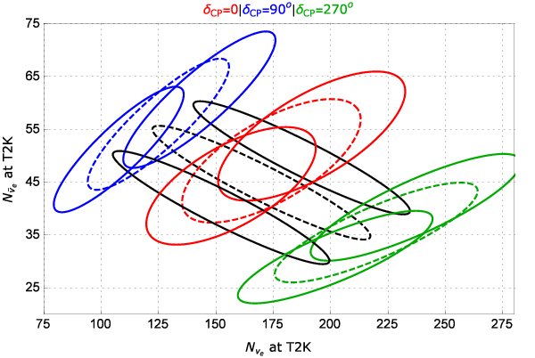
An intuitive plot to illustrate this fact is presented in Fig. 6 where we show the event rates for the neutrino and antineutrino appearance channel in T2K for two different assumptions: the standard three–neutrino case with varying $\delta_{CP}$ (black line), and the alternative non-unitary case with fixed $\delta_{CP}$ and varying $\phi$ (color lines). The variation of the atmospheric angle $\theta_{a}$ has been also considered in the non-unitary case. In particular, dashed lines in the plot correspond to maximal mixing, $\sin^{2}\theta_{a}=0.5$, while solid lines cover approximately the 1$\sigma$ allowed range, $\sin^{2}\theta_{a}=0.5\pm 0.055$. A similar plot was presented in [22] for $L/E=500$, in order to understand the origin of the ambiguity in parameter space which is inherent to the problem. Now we show that, for the same baseline $L/E\approx 500$ m/MeV, the uncertainties in the atmospheric mixing angle spoil the good sensitivity to $\delta_{CP}$ found after the combination of neutrino and antineutrino channel in Ref. [22]. Moreover, one should keep in mind that, in a realistic case, the existence of flux uncertainties would change each of the ellipses of Fig. 6 into bands.

The reason that the leptonic Dirac CP phase $\delta_{CP}$ can be faked by non-unitarity at T2(H)K is due to the choice of narrow neutrino energy spectrum with peak around 550 MeV and baseline at 295 km. With this choice, the oscillation phase $\Phi_{a}\approx\pi/2$ is almost maximal and the $\cos\delta_{CP}$ term vanishes with its coefficient $\cos\Phi_{a}$. It is still easy for the CP phase $\phi$ associated to non-unitarity to fake the standard Dirac phase $\delta_{CP}$, even at the special point pointed in [22], where the degeneracies cancel out in the ideal case of precisely known $\theta_{a}$ and monochromatic energy spectrum. The faking of the standard Dirac CP phase comes from the interplay of various elements. Around the maximal oscillation phase, $\Phi_{a}\approx\pi/2$, the oscillation probability for neutrinos and anti-neutrinos can be approximated by,

where the first line is the same both for neutrino and anti-neutrino modes, while the second receives a minus sign. To fit the current experimental best value $\delta^{true}_{CP}=-\pi/2$ with the opposite $\delta^{fit}_{CP}=\pi/2$, the major difference is introduced by the $\sin$ terms in the second line. The CP sensitivity is spoiled by freeing $\theta_{a}$ and $|\alpha_{21}|$ and it can be faked by varying $\phi$. This introduces a common correction via the $\cos(\phi+\delta_{CP})$ term for both neutrino and anti-neutrino channels. The large uncertainty in the atmospheric angle, which can reach $10\%$ in $s^{2}_{a}$, helps to absorb this common correction. The remaining $\sin\phi$ and $\sin(\phi+\delta_{CP})$ terms can then fake the genuine CP term $\sin\delta_{CP}$. Although the coefficients of $\sin\phi$ and $\sin(\phi+\delta_{CP})$ are relatively small, they are not zero. As long as $\alpha_{21}$ is large enough, CP can be faked. This can explain the behavior seen in Fig. 5 and Fig. 6.

In order to fully resolve the degeneracy between the unitary and non-unitary CP phases, it is necessary to bring back the $\cos\delta_{CP}$ dependence by carefully choosing the energy spectrum and baseline configuration. A perfect candidate for achieving this is to use muon decay at rest ($\mu$DAR) which has a wide peak and shorter baseline around 15-23 km. The TNT2K experiment [13] is proposed to supplement the existing Super-K detector and the future Hyper-K detector with a $\mu$DAR source. Since the accelerator neutrinos in T2(H)K have higher energy than those of the $\mu$DAR source, the two measurements can run simultaneously. Note that for T2K we use the current configuration as described in Sec. IV, while for T2HK the $7.8\times 10^{21}\mbox{POT}$ flux is assigned to neutrino mode only. On the other hand, the $\mu$DAR source can contribute a flux of $1.1\times 10^{25}\mbox{POT}$ [13]. Notice that this experiment has backgrounds from atmospheric neutrinos, from the elastic scattering with electrons, and the quasi-elastic scattering with heavy nuclei. In addition, the $\mu$DAR flux can have 20% uncertainty if there is no near detector.

Note also that the sensitivity to break the degeneracy between $\delta_{CP}$ and $\pi-\delta_{CP}$ at T2(H)K, arising from the single $\sin\delta_{CP}$ dependence, can be improved because of the wide spectrum of $\mu$DAR, which has both $\cos\delta_{CP}$ and $\sin\delta_{CP}$ dependences as shown in Fig. 7.

For the $\mu$DAR flux, the spectrum peaks around 40-50 MeV. In this energy range, the decomposed coefficients $P^{(2)}_{\mu e,e\mu}$ for the $\cos\delta_{CP}$ dependence have comparable magnitude with the $\sin\delta_{CP}$ term coefficients $P^{(3)}_{\mu e,e\mu}$. In contrast, for T2(H)K the coefficients $P^{(2)}_{\mu e,e\mu}$ vanish around the spectrum peak $\sim 550$ MeV while $P^{(3)}_{\mu e,e\mu}$ have sizable magnitude, as shown in Fig. 1.

The property of having both $\cos\delta_{CP}$ and $\sin\delta_{CP}$ dependences is exactly what we need also to break the degeneracy between the unitary and non-unitary CP phases. As shown in Fig. 8, supplementing T2K with $\mu$SK can preserve the CP sensitivity at the T2K level even if not imposing the prior constraint (6). With the prior constraint, the CP sensitivity can further improve beyond that of T2K alone for unitary mixing. The same holds for the T2HK configuration. Nevertheless, the advantage of $\mu$DAR is still not fully utilized.

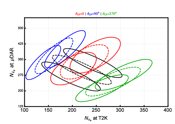
An important difference between T2(H)K in Fig. 5 and TNT2K in Fig. 8 is the effect of adding the prior constraint. At T2(H)K, the prior constraint can only add some moderate improvement. On the other hand, its effect can be maximized at TNT2K after including $\mu$Kam. We find that the CP sensitivity is significantly improved by the combination of $\mu$Kam and prior constraints. Notice in Fig. 9 that the ambiguity of the ellipses was not improved by having another experiment, nevertheless one can distinguish the standard case from the non-unitary case by taking a closer look at the neutrino spectrum which contains more information.

Indeed, the advantage of $\mu$Kam is not fully explored with the current prior constraint in (6). Since the non-unitary CP effect is modulated by $|\alpha_{21}|$, a more stringent constraint on $|\alpha_{21}|$ would effectively suppress the size of the faked CP violation. From the expression of $P^{NP}_{\mu e}$ in Eq. (24c), one sees that if the oscillation baseline is extremely short, it is dominated by the last term

which is a nonzero constant. Such “zero–distance effect” is a direct measure of the effective non–orthonormality of weak–basis neutrinos [47, 48]. Although $P^{NP}_{\mu e}$ is suppressed by $|\alpha_{21}|^{2}$, which is smaller than $6.6\times 10^{-4}$ at 90% C.L., a near detector with a very short baseline can still collect enough number of events to provide information of this parameter.

We propose a near detector $\mu$Near, with a 20 ton scintillator detector and a 20 m baseline to the $\mu$DAR source, to supplement the $\mu$Kam part of TNT2K. By selecting events with double coincidence, the scintillator can identify the oscillated electron anti-neutrinos. Most of the events come from two sources: the signal from $\mu^{+}$ decay and the background from $\mu^{-}$ decay. For both signal and background, the parent muons decay at rest and hence have well–defined spectrum as shown in the left panel of Fig. 10. For a background-signal flux ratio $\mu^{-}\mbox{DAR}/\mu^{+}\mbox{DAR}=5\times 10^{-4}$ [13] and non-unitary size $|\alpha_{21}|=0.02$, the signal and background have roughly the same number of events, $N_{sig}=1446$ and $N_{bkg}=1234$. If the neutrino mixing is unitary, only background is present. Based on this we can roughly estimate the sensitivity at $\mu$Near to be, $\sqrt{N_{bkg}}/N_{sig}\approx 2.4\%$, for $|\alpha_{21}|^{2}=(0.02)^{2}$. When converted to $|\alpha_{21}|$, the limit can be improved by a factor of $1/\sqrt{2.4\%}\approx 6.5$ on the basis of $0.02$ around $1\,\sigma$. In addition, the spectrum shape is quite different between the signal and background. The signal peak appears around 50 MeV where the background event rate is much smaller. This feature of different energy spectrum can further enhance the sensitivity than the rough estimation from total event rate. The constraint on $|\alpha_{21}|$ can be significantly improved beyond the current limit in (6).

In the right panel of Fig. 10 we show the sensitivity on $|\alpha_{21}|$ as a function of the background rate and the detector size from a simplified template fit. The result for $5\times 10^{-4}$ of background and 20 ton detector is of the same size as the rough estimation. The concrete value, $|\alpha_{21}|<0.004$ at 1 $\sigma$, is lightly larger due to marginalization. In Fig. 10 we assumed systematic errors to be 20% for the $\mu$DAR flux normalization and 50% for the background-signal flux ratio. The solid contours in the right panel are obtained with both systematic errors imposed while the dashed ones with only the 20% uncertainty in flux normalization. The difference in the sensitivity on $|\alpha_{21}|$ only appears in the region of small detector size or small background rate. For the 20 ton detector and background rate larger than $10^{-4}$, the difference is negligibly small. In the full simulation, we only implement the 20% uncertainty in flux normalization for simplicity.

In Fig. 11 we show the CP sensitivity at TNT2K plus $\mu$Near once a full simulation is performed. Imposing all the information we can get from TNT2K, $\mu$Near, and the prior constraint on the non-unitary mixing parameters (6), the CP sensitivity can match the full potential of TNT2K under the assumption of unitary mixing. Even without the prior constraint, the CP sensitivity at TNT2K plus $\mu$Near is very close to the full reach of TNT2K with unitary mixing. Imposing the prior constraint (6) has little effect since the constraint on $\alpha_{21}$ from the $\mu$Near detector can be better by one order of magnitude. This combination of CP measurements, TNT2K plus $\mu$Near, can determine the leptonic Dirac CP phase $\delta_{CP}$ unambiguously and hence provide an ultimate solution to the degeneracy between unitary and non-unitary CP violation parameters.

Our interpretation of experimental data always relies on theoretical assumptions. Unambiguous understanding of reality always requires distinguishing alternative assumptions through careful experimental design. The degeneracy between unitary and non-unitary CP phases in neutrino mixing provides a perfect example. In this paper we have confirmed, in agreement with Ref. [22], that, for values of $|\alpha_{21}|$ of the order of a few%, one can have unitarity violating CP oscillation amplitudes of the same order, or possibly larger, than the standard one associated to $\delta_{CP}$. We have illustrated how the CP sensitivity at accelerator neutrino experiments like T2(H)K is severely degraded in the presence of non-unitarity. Indeed, in addition to the standard leptonic Dirac CP phase $\delta_{CP}$ if neutrino mixing is non-unitary there is an extra CP phase $\phi$ characterizing deviations from unitarity and affecting the neutrino appearance probability. The effect of such unitary phase $\delta_{CP}$ can be easily faked by the non-unitarity phase $\phi$ if only the $\sin\delta_{CP}$ dependence is probed, as in the T2(H)K configuration. Probing the interplay with the $\cos\delta_{CP}$ dependence can help to lift the degeneracy.

A perfect solution comes from the TNT2K project with T2(H)K supplemented by a $\mu$DAR source. Thanks to the different energy scale of the accelerator and $\mu$DAR neutrino fluxes, two different measurements can proceed at the same time, using Super-K and Hyper-K detectors simultaneously. In its original proposal, the goal was to get better measurement of the Dirac CP phase $\delta_{CP}$ within the standard three-neutrino mixing benchmark. We find that it also has the potential of breaking the degeneracy between standard and non-unitary CP phases. However, TNT2K can fully explore its advantage only in combination with a near detector. We propose using $\mu$Near, with only 20 ton of scintillator and 20 m of baseline, to monitor the size of the non-unitary CP violating term for the $\mu\to e$ transition, $|\alpha_{21}|$. Our simplified template fit shows that $\mu$Near, with an expected background-signal flux ratio in the $\mu$DAR source of $5\times 10^{-4}$, can constrain $|\alpha_{21}|$ to be smaller than $4\times 10^{-3}$ at $1\,\sigma$, which corresponds to almost one order of magnitude improvement with respect to the current model-independent bound obtained from NOMAD data. This estimate is stable against the large uncertainty in the background-signal flux ratio. When implemented in a full simulation, $\mu$Near can almost retrieve the CP sensitivity of TNT2K, providing an ultimate solution to the degeneracy between unitary and non-unitary mixing parameters.

In short, non-unitary neutrino mixing is expected in a large class of seesaw schemes at LHC–accessible mass scales. This implies extra mixing parameters, and a new CP phase, that can fake the standard leptonic CP phase $\delta_{CP}$ present in the simplest three-neutrino paradigm. As a result, probing for CP violation in accelerator-type experiments can be misleading. We have considered T2(H)K as an example to illustrate the degeneracy between the “standard” and “non-unitary” CP phases. Despite the complete loss in its CP sensitivity we note that supplementing T2(H)K with a $\mu$DAR source can help breaking the CP degeneracy, by probing separately both $\cos\delta_{CP}$ and $\sin\delta_{CP}$ dependences in the wide energy spectrum of the $\mu$DAR flux. We have seen that the further addition of a near detector to the $\mu$DAR setup has the potential of removing the degeneracy rather well.

Work supported by Spanish grants FPA2014-58183-P, Multidark CSD2009-00064, SEV-2014-0398 (MINECO), PROMETEOII/2014/084 (Generalitat Valenciana). M. T. is supported by a Ramón y Cajal contract (MINECO). P. S. P. would like to thank the support of FAPESP funding grant 2014/05133-1, 2015/16809-9 and 2014/19164-6. SFG thanks Jarah Evslin for useful discussions.

References

- [1] G. Branco, R. G. Felipe, and F. Joaquim, Rev.Mod.Phys. 84, 515 (2012), arXiv:1111.5332 [hep-ph] .
- [2] P. Chen, G.-J. Ding, F. Gonzalez-Canales, and J. W. F. Valle, (2016a), arXiv:1604.03510 [hep-ph] .
- [3] P. Chen, G.-J. Ding, F. Gonzalez-Canales, and J. W. F. Valle, Phys. Lett. B753, 644 (2016b), arXiv:1512.01551 [hep-ph] .
- [4] S. Morisi and J. W. F. Valle, Fortsch.Phys. 61, 466 (2013), arXiv:1206.6678 [hep-ph] .
- [5] S. F. King, A. Merle, S. Morisi, Y. Shimizu, and M. Tanimoto, New J. Phys. 16, 045018 (2014), arXiv:1402.4271 [hep-ph] .
- [6] M. Kobayashi and T. Maskawa, Prog. Theor. Phys. 49, 652 (1973).
- [7] J. Schechter and J. W. F. Valle, Phys. Rev. D22, 2227 (1980).
- [8] L. Wolfenstein, Phys. Rev. Lett. 51, 1945 (1983).
- [9] M. Maltoni, T. Schwetz, M. Tortola, and J. Valle, New J.Phys. 6, 122 (2004), arXiv:hep-ph/0405172 [hep-ph] .
- [10] D. V. Forero, M. Tortola, and J. W. F. Valle, Phys. Rev. D90, 093006 (2014), arXiv:1405.7540 [hep-ph] .
- [11] K. Abe et al. (T2K), Phys. Rev. D91, 072010 (2015a), arXiv:1502.01550 [hep-ex] .
- [12] K. Abe et al., (2011), arXiv:1109.3262 [hep-ex] .
- [13] J. Evslin, S.-F. Ge, and K. Hagiwara, JHEP 02, 137 (2016), arXiv:1506.05023 [hep-ph] .
- [14] R. N. Mohapatra and J. W. F. Valle, Phys. Rev. D34, 1642 (1986).
- [15] M. Gonzalez-Garcia and J. Valle, Phys.Lett. B216, 360 (1989).
- [16] E. K. Akhmedov, M. Lindner, E. Schnapka, and J. W. F. Valle, Phys. Rev. D53, 2752 (1996a), arXiv:hep-ph/9509255 [hep-ph] .
- [17] E. K. Akhmedov, M. Lindner, E. Schnapka, and J. Valle, Phys.Lett. B368, 270 (1996b), arXiv:hep-ph/9507275 [hep-ph] .
- [18] M. Malinsky, J. Romao, and J. Valle, Phys.Rev.Lett. 95, 161801 (2005), arXiv:hep-ph/0506296 [hep-ph] .
- [19] F. Bazzocchi, Phys.Rev. D83, 093009 (2011), arXiv:1011.6299 [hep-ph] .
- [20] F. J. Escrihuela, D. V. Forero, O. G. Miranda, M. Tortola, and J. W. F. Valle, Phys. Rev. D92, 053009 (2015), arXiv:1503.08879 [hep-ph] .
- [21] Y.-F. Li and S. Luo, Phys. Rev. D93, 033008 (2016), arXiv:1508.00052 [hep-ph] .
- [22] O. G. Miranda, M. Tortola, and J. W. F. Valle, (2016), arXiv:1604.05690 [hep-ph] .
- [23] O. G. Miranda and J. W. F. Valle, (2016), arXiv:1602.00864 [hep-ph] .
- [24] S.-F. Ge, H.-J. He, and F.-R. Yin, JCAP 1005, 017 (2010), arXiv:1001.0940 [hep-ph] .
- [25] H.-J. He and F.-R. Yin, Phys.Rev. D84, 033009 (2011), arXiv:1104.2654 [hep-ph] .
- [26] D. A. Dicus, S.-F. Ge, and W. W. Repko, Phys. Rev. D83, 093007 (2011), arXiv:1012.2571 [hep-ph] .
- [27] S.-F. Ge, D. A. Dicus, and W. W. Repko, Phys. Lett. B702, 220 (2011), arXiv:1104.0602 [hep-ph] .
- [28] S.-F. Ge, D. A. Dicus, and W. W. Repko, Phys. Rev. Lett. 108, 041801 (2012), arXiv:1108.0964 [hep-ph] .
- [29] A. D. Hanlon, S.-F. Ge, and W. W. Repko, Phys. Lett. B729, 185 (2014), arXiv:1308.6522 [hep-ph] .
- [30] H.-J. He, W. Rodejohann, and X.-J. Xu, Phys. Lett. B751, 586 (2015), arXiv:1507.03541 [hep-ph] .
- [31] J. Bernabeu et al., Phys. Lett. B187, 303 (1987).
- [32] G. C. Branco, M. N. Rebelo, and J. W. F. Valle, Phys. Lett. B225, 385 (1989).
- [33] N. Rius and J. W. F. Valle, Phys. Lett. B246, 249 (1990).
- [34] F. Deppisch and J. W. F. Valle, Phys. Rev. D72, 036001 (2005), hep-ph/0406040 .
- [35] F. Deppisch, T. S. Kosmas, and J. W. F. Valle, Nucl. Phys. B752, 80 (2006), hep-ph/0512360 .
- [36] F. F. Deppisch, N. Desai, and J. W. F. Valle, Phys.Rev. D89, 051302(R) (2014), arXiv:1308.6789 [hep-ph] .
- [37] S. Das, F. Deppisch, O. Kittel, and J. W. F. Valle, Phys.Rev. D86, 055006 (2012), arXiv:1206.0256 [hep-ph] .
- [38] S. Mikheev and A. Smirnov, Sov.J.Nucl.Phys. 42, 913 (1985).
- [39] L. Wolfenstein, Phys.Rev. D17, 2369 (1978).
- [40] S.-F. Ge, NuPro: a simulation package for neutrino properties, http://nupro.hepforge.org (to appear).
- [41] J. W. Valle and J. C. Romao, Neutrinos in high energy and astroparticle physics (John Wiley & Sons, 2015).
- [42] K. A. Olive et al. (Particle Data Group), Chin. Phys. C38, 090001 (2014).
- [43] J. Schechter and J. W. F. Valle, Phys. Rev. D23, 1666 (1981).
- [44] M. Doi, T. Kotani, H. Nishiura, K. Okuda, and E. Takasugi, Phys. Lett. B102, 323 (1981).
- [45] J. Schechter and J. Valle, Phys.Rev. D25, 2951 (1982a).
- [46] J. Schechter and J. W. F. Valle, Phys. Rev. D25, 774 (1982b).
- [47] J. W. F. Valle, Phys. Lett. B199, 432 (1987).
- [48] H. Nunokawa et al., Phys. Rev. D54, 4356 (1996), hep-ph/9605301 .
- [49] S. Antusch, C. Biggio, E. Fernandez-Martinez, M. B. Gavela, and J. Lopez-Pavon, JHEP 10, 084 (2006), arXiv:hep-ph/0607020 [hep-ph] .
- [50] S.-F. Ge, K. Hagiwara, and C. Rott, JHEP 06, 150 (2014), arXiv:1309.3176 [hep-ph] .
- [51] K. Abe et al. (T2K), PTEP 2015, 043C01 (2015b), arXiv:1409.7469 [hep-ex] .
- [52] E. K. Akhmedov, A. Dighe, P. Lipari, and A. Y. Smirnov, Nucl. Phys. B542, 3 (1999), arXiv:hep-ph/9808270 [hep-ph] .
- [53] H. Yokomakura, K. Kimura, and A. Takamura, Phys. Lett. B544, 286 (2002), arXiv:hep-ph/0207174 [hep-ph] .