跳到论文正文
W Papers独立论文阅读器 arXiv:1605.01606 论文正文 计算阅读时间 · 0%
引用这篇论文根据当前论文元数据生成,正式投稿前建议核对。


License: arXiv.org perpetual non-exclusive license
arXiv:1605.01606v2 [math.OC] 06 Jun 2017

Event-Triggered Cooperative Robust Practical Output Regulation for a Class of Linear Multi-Agent Systems footnoteinfo

Wei Liu Email: wliu@mae.cuhk.edu.hk    Jie Huang Email: jhuang@mae.cuhk.edu.hk
Abstract

In this paper, we consider the event-triggered cooperative robust practical output regulation problem for a class of linear minimum-phase multi-agent systems. We first convert our problem into the cooperative robust practical stabilization problem of a well defined augmented system Based on the distributed internal model approach. Then, we design a distributed event-triggered output feedback control law together with a distributed output-based event-triggered mechanism to stabilize the augmented system, which leads to the solvability of the cooperative robust practical output regulation problem of the original plant. Our distributed control law can be directly implemented in a digital platform provided that the distributed triggering mechanism can monitor the continuous-time output information from neighboring agents. Finally, we illustrate our design by an example.

keywords
Cooperative output regulation, event-triggered control, linear multi-agent systems, robust control.
††thanks: [††address: Department of Mechanical and Automation Engineering, The Chinese University of Hong Kong, Shatin, N.T., Hong Kong

footnoteinfo]This work has been supported in part by the Research Grants Council of the Hong Kong Special Administration Region under grant No. 14200515, and in part by National Natural Science Foundation of China under Project 61633007. Corresponding author: Jie Huang.

,

1 Introduction

Over the past few years, event-triggered control has attracted extensive attention from the control community. Compared with conventional periodical time-triggered control, event-triggered control samples the system’s state or output aperiodically and reduces the number of control task executions while maintaining the control performance. As noted in [8], event-triggered control is reactive and generates sensor sampling and control actuation when, for instance, the plant state or output deviates more than a certain threshold from a desired value. Various event-triggered control problems have been studied for several types of systems in [5, 7, 12, 13, 19, 20] and the references therein. One of the main challenges for event-triggered control is to avoid the Zeno behavior, which means that the execution times become arbitrarily close and result in an accumulation point [19]. In [19], the stabilization problem of a given system by a state-based event-triggered control law was linked to the input-to-state stabilizability (ISS) of the system, and it was shown that the Zeno behavior can be excluded when the measurement state is not equal to zero. In [7], a dynamic state-based event-triggered mechanism was further proposed to study the stabilization problem for the same class of nonlinear systems as that in [19]. Reference [20] studied the asymptotic tracking problem of a control system by a stated-based event-triggered controller and it gave a stated-based event-triggered controller that was able to achieve the uniform ultimate boundedness of the tracking error. Reference [12] further studied the robust stabilization problem for a class of systems subject to external disturbances by a state-based event-triggered control based on the small-gain theorem. In [5], an output-based event-triggered control law was proposed to analyze the stability and ℒ∞\mathcal{L}_{\infty} performance for a class of linear systems. In [13], the robust practical output regulation problem for a class of linear systems was studied by an output-based event-triggered control law. Some other contributions can also be found in [1, 4, 16] etc.

In this paper, we further consider the cooperative robust practical output regulation problem for a class of linear minimum-phase multi-agent systems by a dynamic distributed output-based event-triggered control law. The problem can be viewed as an extension of the result in [13] from a single system to a multi-agent system. Compared with [13], the main challenge for this paper is that the control of each subsystem and hence the triggering mechanism are subject to some communication constraints described by a digraph. We need to specifically design an output-based event-triggered control law that satisfies the communication constraints. Thus, our problem is more challenging than that of [13]. In what follows, a control law and an event-triggered mechanism satisfying the communication constraints are called a distributed control law and a distributed event-triggered mechanism, respectively.

Several other cooperative control problems of multi-agent systems by event-triggered control have also been studied. For example, the consensus problem of single-integrator and double-integrator multi-agent systems by event-triggered control was studied in [3, 6, 17], and [11, 14], respectively. Reference [23] studied the consensus problem for the general linear multi-agent systems by an observer-based output feedback event-triggered distributed control law. Reference [21] studied the cooperative output regulation problem for linear multi-agent system by a centralized event-triggered mechanism. Reference [10] further studied the cooperative output regulation problem for linear multi-agent systems by a distributed event-triggered mechanism based on the feedforward design method. Other relevant results for the general linear multi-agent systems can be found in [2, 22, 24] etc.

Compared with the existing results on event-triggered cooperative control problems, this paper needs to overcome some specific challenges. First, our problem formulation generalizes the existing event-triggered cooperative control problems, say, in [2, 3, 6, 11, 14, 17, 23, 24], in the sense that we achieve not only asymptotical tracking but also disturbance rejection. Second, since our system contains unknown parameters, we need to adopt the distributed internal model approach, which leads to a robust stabilization problem for a much more complicated augmented system. Third, our event-triggered mechanism is output-based and distributed in the sense that the event-triggered mechanism of each agent only depends on the output information of its neighbors and itself. Finally, our control law is piecewise constant, which lends itself to a direct implementation in a digital platform.

Throughout this paper, we use the following notation: ℤ+\mathbb{Z}^{+} denotes the set of all nonnegative integers. For any column vectors aia_{i}, i=1,…,si=1,...,s, we denote col​(a1,…,as)=[a1T,…,asT]T\mbox{col}(a_{1},...,a_{s})=[a_{1}^{T},...,a_{s}^{T}]^{T}. For any matrices X∈ℝn×mX\in\mathbb{R}^{n\times m}, we denote vec​(X)=[X1T,⋯,XmT]T\mbox{vec}(X)=[X_{1}^{T},\cdots,X_{m}^{T}]^{T} where XiX_{i} with i=1,⋯,mi=1,\cdots,m is the iith column of XX. The notation ‖x‖\|x\| denotes the Euclidean norm of vector xx. The notation ‖A‖\|A\| denotes the induced norm of matrix AA by the Euclidean norm. The notation ⊗\otimes denotes the Kronecker product of matrices. Denote the base of the natural logarithm by 𝐞\mathbf{e}. Denote the maximum eigenvalue and the minimum eigenvalue of a symmetric real matrix AA by λmax​(A)\lambda_{\max}(A) and λmin​(A)\lambda_{\min}(A), respectively.

2 Problem formulation and preliminaries

Consider the following linear multi-agent systems

z˙i=A1​i​(w)​zi+A2​i​(w)​ξ1​i+E0​i​(w)​vξ˙s​i=ξ(s+1)​i,s=1,⋯,r−1ξ˙r​i=A3​i​(w)​zi+∑s=1rcs​i​(w)​ξs​i+Er​i​(w)​v+bi​(w)​uiyi=ξ1​i,i=1,⋯,N,\begin{split}&\dot{z}_{i}=A_{1i}(w)z_{i}+A_{2i}(w)\xi_{1i}+E_{0i}(w)v\\ &\dot{\xi}_{si}=\xi_{(s+1)i},\ \ s=1,\cdots,r-1\\ &\dot{\xi}_{ri}\!=\!A_{3i}(w)z_{i}\!+\!\sum_{s=1}^{r}c_{si}(w)\xi_{si}\!+\!E_{ri}(w)v\!+\!b_{i}(w)u_{i}\\ &y_{i}=\xi_{1i},\ i=1,\cdots,N,\end{split} (1)

where zi∈ℝni−rz_{i}\in\mathbb{R}^{n_{i}-r} and ξi=col​(ξ1​i,⋯,ξr​i)∈ℝr\xi_{i}=\mbox{col}(\xi_{1i},\cdots,\xi_{ri})\in\mathbb{R}^{r} are the states, ui∈ℝu_{i}\in\mathbb{R} is the input, yi∈ℝy_{i}\in\mathbb{R} is the output, w∈ℝnww\in\mathbb{R}^{n_{w}} is an unknown parameter vector, bi​(w)>0b_{i}(w)>0 for all w∈ℝnww\in\mathbb{R}^{n_{w}}, and v⁡(t)∈ℝnvv(t)\in\mathbb{R}^{n_{v}} is an exogenous signal representing both reference input and disturbance and is assumed to be generated by the following linear system

v˙=S​v\begin{split}\dot{v}=Sv\end{split} (2)

where SS is some known constant matrix. Let y0=F⁡(w)​v∈ℝy_{0}=F(w)v\in\mathbb{R} be the output of the exosystem (2). Then, the regulated error of each subsystem is defined as ei=yi−y0e_{i}=y_{i}-y_{0} for i=1,⋯,Ni=1,\cdots,N.

For i=1,⋯,Ni=1,\cdots,N and s=1,⋯,rs=1,\cdots,r, let A1​i​(w)=A1+wA1​i∈ℝ(ni−r)×(ni−r)A_{1i}(w)=A_{1}+w_{A_{1i}}\in\mathbb{R}^{(n_{i}-r)\times(n_{i}-r)}, A2​i​(w)=A2+wA2​i∈ℝ(ni−r)×1A_{2i}(w)=A_{2}+w_{A_{2i}}\in\mathbb{R}^{(n_{i}-r)\times 1}, A3​i​(w)=A3+wA3​i∈ℝ1×(ni−r)A_{3i}(w)=A_{3}+w_{A_{3i}}\in\mathbb{R}^{1\times(n_{i}-r)}, E0​i​(w)=E0+wE0​i∈ℝ(ni−r)×nvE_{0i}(w)=E_{0}+w_{E_{0i}}\in\mathbb{R}^{(n_{i}-r)\times n_{v}}, Er​i​(w)=Er+wEr​i∈ℝ1×nvE_{ri}(w)=E_{r}+w_{E_{ri}}\in\mathbb{R}^{1\times n_{v}}, F⁡(w)=F+wF∈ℝ1×nvF(w)\!=\!F\!+\!w_{F}\in\mathbb{R}^{1\times n_{v}}, cs​i​(w)=cs+wcs​i∈ℝc_{si}(w)=c_{s}\!+\!w_{c_{si}}\in\mathbb{R}, bi​(w)=b+wbi∈ℝb_{i}(w)\!=\!b+w_{b_{i}}\in\mathbb{R}, wA1=col​(vec​(wA11),⋯,vec​(wA1​N))w_{A_{1}}\!\!=\!\mbox{col}(\mbox{vec}(w_{A_{11}}),\cdots,\mbox{vec}(w_{A_{1N}})), wA2=w_{A_{2}}\!\!= col​(vec​(wA21),⋯,vec​(wA2​N))\mbox{col}(\mbox{vec}(w_{A_{21}}),\cdots\!,\mbox{vec}(w_{A_{2N}})), wA3=col​(vec​(wA31),⋯CLOSEw_{A_{3}}\!\!=\!\mbox{col}(\mbox{vec}(w_{A_{31}}),\cdots, OPENvec​(wA3​N))\mbox{vec}(w_{A_{3N}})), wE0=w_{E_{0}}\!\!=\! col​(vec​(wE01),⋯,vec​(wE0​N))\mbox{col}(\mbox{vec}(w_{E_{01}}),\cdots,\mbox{vec}(w_{E_{0N}})), wErw_{E_{r}} =col​(vec​(wEr​1),⋯,vec​(wEr​N))=\mbox{col}(\mbox{vec}(w_{E_{r1}}),\cdots,\mbox{vec}(w_{E_{rN}})), wcs=col​(wcs​1,⋯CLOSEw_{c_{s}}=\mbox{col}(w_{c_{s1}},\cdots, OPENwcs​N)w_{c_{sN}}), wb=col​(wb1,⋯,wbN)w_{b}=\mbox{col}(w_{b_{1}},\cdots,w_{b_{N}}), w=col​(wA1,wA2,wA3CLOSEw=\mbox{col}(w_{A_{1}},w_{A_{2}},w_{A_{3}}, OPENwE0,wEr,wc1,⋯,wcr,wb,wFT)w_{E_{0}},w_{E_{r}},w_{c_{1}},\cdots,w_{c_{r}},w_{b},w_{F}^{T}), where A1,A2,A3,E0A_{1},A_{2},A_{3},E_{0}, Er,F,csE_{r},F,c_{s} and bb denote the nominal values, and ww denotes the unknown parameter.

System (1) is called a linear multi-agent system in the normal form and it is said to be minimum phase if the matrix A1​i​(w)A_{1i}(w) is Hurwitz for all ww. Systems (1) and (2) together can be viewed as a multi-agent system with (2) as the leader system, and the NN subsystems of (1) as NN followers. It is noted that the cooperative robust output regulation problem for the multi-agent system composed of (1) and (2) was studied by the continuous distributed control law in [18].

As in [18], given the plant (1) and the exosystem (2), we can define a digraph 𝒢¯=(𝒱¯,ℰ¯)\bar{\mathcal{G}}=(\bar{\mathcal{V}},\bar{\mathcal{E}})11 1 See [18] for a summary of digraph., where 𝒱¯={0,1⋯,N}\bar{\mathcal{V}}=\{0,1\cdots,N\} with 00 associated with the leader system and with i=1,⋯,Ni=1,\cdots,N associated with the NN followers, respectively, and ℰ¯⊆𝒱¯×𝒱¯\bar{\mathcal{E}}\subseteq\bar{\mathcal{V}}\times\bar{\mathcal{V}} for all t≥0t\geq 0. For all t≥0t\geq 0, each j=0,1,⋯,Nj=0,1,\cdots,N, i=1,⋯,Ni=1,\cdots,N, and i≠ji\neq j, (j,i)∈ℰ¯(j,i)\in\bar{\mathcal{E}} if and only if the control ui​(t)u_{i}(t) can make use of yi​(t)−yj​(t)y_{i}(t)-y_{j}(t) for feedback control. Let 𝒩¯i={j,(j,i)∈ℰ¯}\bar{\mathcal{N}}_{i}=\{j,(j,i)\in\bar{\mathcal{E}}\} denote the neighbor set of node ii.

To define our control law, we recall that the adjacency matrix of the digraph 𝒢¯\bar{\mathcal{G}} is a nonnegative matrix 𝒜¯=[a¯i​j]∈ℝ(N+1)×(N+1)\bar{\mathcal{A}}=[\bar{a}_{ij}]\in\mathbb{R}^{(N+1)\times(N+1)} where a¯i​i=0\bar{a}_{ii}=0, a¯i​j=1⇔(j,i)∈ℰ¯\bar{a}_{ij}=1\Leftrightarrow(j,i)\in\mathcal{\bar{E}}, and a¯i​j=0⇔(j,i)∉ℰ¯\bar{a}_{ij}=0\Leftrightarrow(j,i)\notin\mathcal{\bar{E}} for i,j=0,1,⋯,Ni,j=0,1,\cdots,N. Like in [18], define the virtual output for the iith subsystem as ev​i​(t)=∑j=0Na¯i​j​(yi​(t)−yj​(t))e_{vi}(t)=\sum_{j=0}^{N}\bar{a}_{ij}(y_{i}(t)-y_{j}(t)) for i=1,⋯,Ni=1,\cdots,N. Let e0=0e_{0}=0, e=col​(e1,⋯,eN)e=\mbox{col}(e_{1},\cdots,e_{N}), ev=col​(ev​1,⋯,ev​N)e_{v}=\mbox{col}(e_{v1},\cdots,e_{vN}), and H=[hi​j]i,j=1NH=[h_{ij}]_{i,j=1}^{N} with hi​i=∑j=0Na¯i​jh_{ii}=\sum_{j=0}^{N}\bar{a}_{ij} and hi​j=−a¯i​jh_{ij}=-\bar{a}_{ij} for i≠ji\neq j. It can be verified that ev=H​ee_{v}=He.

For any k∈ℤ+k\in\mathbb{Z}^{+} and i=1,⋯,Ni=1,\cdots,N, consider the following control law

ui​(t)=F1​ηi​(tki)+F2​ζi​(tki)η˙i​(t)=G1​ηi​(t)+G2​ηi​(tki)+G3​ζi​(tki)ζ˙i​(t)=G4​ζi​(t)+G5​ev​i​(tki)\begin{split}&u_{i}(t)=F_{1}\eta_{i}(t_{k}^{i})+F_{2}\zeta_{i}(t_{k}^{i})\\ &\dot{\eta}_{i}(t)=G_{1}\eta_{i}(t)+G_{2}\eta_{i}(t_{k}^{i})+G_{3}\zeta_{i}(t_{k}^{i})\\ &\dot{\zeta}_{i}(t)=G_{4}\zeta_{i}(t)+G_{5}e_{vi}(t_{k}^{i})\\ \end{split} (3)

where F1F_{1}, F2F_{2}, G1,⋯,G5G_{1},\cdots,G_{5} are some real matrices with proper dimensions, the ηi\eta_{i} subsystem is the so-called internal model, the ζi\zeta_{i} subsystem is a dynamic compensator, and tkit_{k}^{i} denotes the triggering time instants of agent ii with t0i=0t_{0}^{i}=0 and is generated by the following event-triggered mechanism:

tk+1i=inf{t>tki|hi​(e~v​i​(t),η~i​(t),ζ~i​(t),ev​i​(t),ζi​(t),t)≥δ}\begin{split}t_{k+1}^{i}\!\!=\!\inf\{t\!>\!t_{k}^{i}|h_{i}(\tilde{e}_{vi}(t),\tilde{\eta}_{i}(t),\tilde{\zeta}_{i}(t),e_{vi}(t),\zeta_{i}(t),t)\!\geq\!\delta\}\end{split} (4)

where hi​(⋅)h_{i}(\cdot) is some nonlinear function, δ>0\delta>0 is a constant and e~v​i​(t)=ev​i​(tki)−ev​i​(t)\tilde{e}_{vi}(t)=e_{vi}(t_{k}^{i})-e_{vi}(t), η~i​(t)=ηi​(tki)−ηi​(t)\tilde{\eta}_{i}(t)=\eta_{i}(t_{k}^{i})-\eta_{i}(t), ζ~i​(t)=ζi​(tki)−ζi​(t)\tilde{\zeta}_{i}(t)=\zeta_{i}(t_{k}^{i})-\zeta_{i}(t).

Remark 2.1

The event-triggering mechanism (4) and the control law (3) are both distributed and output-based, and we call (3) as the dynamic distributed output-based event-triggered control law.

Our problem is described as follows.

Problem 1

Given the plant (1), the exosystem (2), any compact sets 𝕍∈ℝnv\mathbb{V}\in\mathbb{R}^{n_{v}} with 0∈𝕍0\in\mathbb{V} and 𝕎⊂ℝnw\mathbb{W}\subset\mathbb{R}^{n_{w}} with 0∈𝕎0\in\mathbb{W}, a digraph 𝒢¯\bar{\mathcal{G}}, and any ϵ>0\epsilon>0, design an event-triggered mechanism of the form (4) and a control law of the form (3) such that the resulting closed-loop system has the following properties: for any v∈𝕍v\in\mathbb{V}, w∈𝕎w\in\mathbb{W}, and any initial conditions zi​(0)z_{i}(0), ξi​(0)\xi_{i}(0), ηi​(0)\eta_{i}(0), ζi​(0)\zeta_{i}(0) for i=1,⋯,Ni=1,\cdots,N,

a)

the trajectory of the closed-loop system exists and is bounded for all time t≥0t\geq 0;

b)

limt→+∞‖e⁡(t)‖≤ϵ\lim_{t\to+\infty}\|e(t)\|\leq\epsilon.

Remark 2.2

We call Problem 1 as the event-triggered cooperative robust practical output regulation problem. Clearly, Problem 1 is more challenging than the cooperative robust output regulation problem studied in [18] in at least three ways. First, we not only need to design a control law, but also an event-triggered mechanism. Moreover, both the control law and the event-triggered mechanism must be distributed in the sense that both the control law and the event-triggered mechanism of each subsystem can only make use of the information of its neighbors and itself. Second, since the closed-loop system is hybrid under event-triggered control, the stability analysis of the closed-loop system is much more complicated than that of the closed-loop system in [18] which is smooth. Third, we need to make a special effort to design an appropriate event-triggered mechanism to prevent the Zeno phenomenon. It is also interesting to note that, unlike the control laws in [10, 21, 22, 23], the specific form of the control law (3) lends itself to a direct digital implementation as follows:

ui​(t)=F1​ηi​(tki)+F2​ζi​(tki)ηi​(tk+1i)=𝐞G1​(tk+1i−tki)​ηi​(tki)+(G2​ηi​(tki)+G3​ζi​(tki))​∫tkitk+1i𝐞G1​(tk+1i−τ)​𝑑τζi​(tk+1i)=𝐞G4​(tk+1i−tki)​ζi​(tki)+G5​ev​i​(tki)​∫tkitk+1i𝐞G4​(tk+1i−τ)​𝑑τ\begin{split}u_{i}(t)\!=&F_{1}\eta_{i}(t_{k}^{i})+F_{2}\zeta_{i}(t_{k}^{i})\\ \eta_{i}(t_{k+1}^{i})\!=&\mathbf{e}^{G_{1}(t_{k+1}^{i}-t_{k}^{i})}\eta_{i}(t_{k}^{i})+\\ &(G_{2}\eta_{i}(t_{k}^{i})\!+\!G_{3}\zeta_{i}(t_{k}^{i}))\!\!\!\int_{t_{k}^{i}}^{t_{k+1}^{i}}\!\!\!\mathbf{e}^{G_{1}(t_{k+1}^{i}\!-\!\tau)}d\tau\\ \zeta_{i}(t_{k+1}^{i})\!=&\mathbf{e}^{G_{4}(t_{k+1}^{i}-t_{k}^{i})}\zeta_{i}(t_{k}^{i})+\\ &G_{5}e_{vi}(t_{k}^{i})\int_{t_{k}^{i}}^{t_{k+1}^{i}}\!\mathbf{e}^{G_{4}(t_{k+1}^{i}-\tau)}d\tau\\ \end{split} (5)

for t∈[tki,tk+1i)t\in[t_{k}^{i},t_{k+1}^{i}) with k∈ℤ+k\in\mathbb{Z}^{+} and i=1,⋯,Ni=1,\cdots,N.

Remark 2.3

It is noted that the event-triggered mechanism (4) relies on the continuous-time measurement output ev​i​(t)e_{vi}(t), thus costing communication resources. It is interesting to further consider how to design novel triggering mechanisms that avoid continuous communication by appropriate samplings.

To solve our problem, we need some assumptions as follows.

Assumption 1

The exosystem is neutrally stable, i.e., all the eigenvalues of S are semi-simple with zero real parts.

Assumption 2

For i=1,⋯,Ni=1,\cdots,N, each subsystem of (1) is minimum phase for any w∈𝕎w\in\mathbb{W}, i.e. A1​i​(w)A_{1i}(w) is Hurwitz for all w∈𝕎w\in\mathbb{W}.

Assumption 3

The digraph 𝒢¯\bar{\mathcal{G}} is connected, i.e., it contains a directed spanning tree with node 00 as the root.

Remark 2.4

Assumption 1 has also been used in [13]. Under Assumption 1, for any v⁡(0)∈𝕍0v(0)\in\mathbb{V}_{0} with 𝕍0\mathbb{V}_{0} being a compact set, there exists another compact set 𝕍\mathbb{V} such that v⁡(t)∈𝕍v(t)\in\mathbb{V} for all t≥0t\geq 0. Assumptions 2 and 3 are the same as Assumptions 6 and 7 of [18]. Under Assumption 3, by Lemma 4 in [9], HH is nonsingular and all eigenvalues of HH have positive real parts.

3 The existing result

In this section, we will summarize the result of [18], where the cooperative robust output regulation problem for the system (1) has been studied by a continuous-time distributed output feedback control law.

As shown in [18], under Assumptions 1-2, we can define a set of dynamic compensators

η˙i=Mηi+Qui,i=1,⋯,N\begin{split}\dot{\eta}_{i}=M\eta_{i}+Qu_{i},\ i=1,\cdots,N\end{split} (6)

where (M,Q)(M,Q) is any controllable pair with M∈ℝl×lM\in\mathbb{R}^{l\times l} being a Hurwitz matrix, Q∈ℝl×1Q\in\mathbb{R}^{l\times 1} being a column vector and ll being the degree of the minimal polynomial of SS. This set of dynamic compensators is called the distributed internal model of the system (1). Let Φ=[01⋯0⋱00⋯1−α0−α1⋯−αl−1]\Phi=\begin{bmatrix}\begin{smallmatrix}0&1&\cdots&0\\ \vdots&\vdots&\ddots&\vdots\\ 0&0&\cdots&1\\ -\alpha_{0}&-\alpha_{1}&\cdots&-\alpha_{l-1}\\ \end{smallmatrix}\end{bmatrix} and Γ=[100]T\Gamma=\begin{bmatrix}\begin{smallmatrix}1\\ 0\\ \vdots\\ 0\\ \end{smallmatrix}\end{bmatrix}^{T}, where α0,α1,⋯,αl−1\alpha_{0},\alpha_{1},\cdots,\alpha_{l-1} are some real numbers such that m⁡(𝐬)=𝐬l+αl−1​𝐬l−1+⋯+α1​𝐬+α0m(\mathbf{s})=\mathbf{s}^{l}+\alpha_{l-1}\mathbf{s}^{l-1}+\cdots+\alpha_{1}\mathbf{s}+\alpha_{0} is the minimal polynomial of SS. Let TT be the unique solution of the following Sylvester equation [15]:

T​Φ−M​T=Q​Γ,\begin{split}T\Phi-MT=Q\Gamma,\end{split} (7)

and, for i=1,⋯,Ni=1,\cdots,N, let Πi​(w)\Pi_{i}(w) be the unique solution of the following Sylvester equation

Πi​(w)​S=A1​i​(w)​Πi​(w)+A2​i​(w)​F​(w)+E0​i​(w).\begin{split}\Pi_{i}(w)S\!=\!A_{1i}(w)\Pi_{i}(w)\!+\!A_{2i}(w)F(w)\!+\!E_{0i}(w).\end{split} (8)

Finally, let Ui​(w)=−bi−1​(w)​(A3​i​(w)​Πi​(w)+Er​i​(w)+∑s=1rcs​i​(w)​F​(w)​Ss−1−F⁡(w)​Sr)U_{i}(w)=-b_{i}^{-1}(w)\big(A_{3i}(w)\Pi_{i}(w)+E_{ri}(w)+\sum_{s=1}^{r}c_{si}(w)F(w)S^{s-1}-F(w)S^{r}\big) and Υi​(w)=col​(Ui​(w),Ui​(w)​SCLOSE\Upsilon_{i}(w)=\mbox{col}(U_{i}(w),U_{i}(w)S, OPEN⋯,Ui​(w)​Sl−1)\cdots,U_{i}(w)S^{l-1}).

Then, as shown in [18], performing on the internal model (6) and the plant (1) the following transformation

z¯i=zi−Πi​(w)​vξ¯s​i=ξs​i−F(w)Ss−1v,s=1,⋯,rη¯i=ηi−T​Υi​(w)​vu¯i=ui−ΓT−1ηi,i=1,⋯,N\begin{split}&\bar{z}_{i}=z_{i}-\Pi_{i}(w)v\\ &\bar{\xi}_{si}=\xi_{si}-F(w)S^{s-1}v,~s=1,\cdots,r\\ &\bar{\eta}_{i}=\eta_{i}-T\Upsilon_{i}(w)v\\ &\bar{u}_{i}=u_{i}-\Gamma T^{-1}\eta_{i},~i=1,\cdots,N\end{split} (9)

leads to the following so-called augmented system

z¯˙i=A1​i​(w)​z¯i+A2​i​(w)​ξ¯1​iξ¯˙s​i=ξ¯(s+1)​i,s=1,⋯,r−1ξ¯˙r​i=A3​i​(w)​z¯i+∑s=1rcs​i​(w)​ξ¯s​i+bi​(w)​u¯i+bi​(w)​Γ​T−1​η¯iη¯˙i=(M+Q​Γ​T−1)​η¯i+Q​u¯i,ei=ξ¯1​i.\begin{split}\dot{\bar{z}}_{i}=&A_{1i}(w)\bar{z}_{i}+A_{2i}(w)\bar{\xi}_{1i}\\ \dot{\bar{\xi}}_{si}=&\bar{\xi}_{(s+1)i},\ s=1,\cdots,r-1\\ \dot{\bar{\xi}}_{ri}=&A_{3i}(w)\bar{z}_{i}+\sum_{s=1}^{r}c_{si}(w)\bar{\xi}_{si}+b_{i}(w)\bar{u}_{i}\\ &+b_{i}(w)\Gamma T^{-1}\bar{\eta}_{i}\\ \dot{\bar{\eta}}_{i}=&(M+Q\Gamma T^{-1})\bar{\eta}_{i}+Q\bar{u}_{i},\\ e_{i}=&\bar{\xi}_{1i}.\end{split} (10)

Then the main result in [18] can be summarized as follows.

Lemma 3.1

Consider the following continuous-time distributed output feedback control law

u¯i​(t)=−K​Ω​ζi​(t)ζ˙i​(t)=Ao(h)ζi(t)+Bo(h)ev​i(t),i=1,⋯,N\begin{split}\bar{u}_{i}(t)&=-K\Omega\zeta_{i}(t)\\ \dot{\zeta}_{i}(t)&=A_{o}(h)\zeta_{i}(t)+B_{o}(h)e_{vi}(t),\ \ i=1,\cdots,N\end{split} (11)

where ζi=col​(ζ1​i,ζ2​i,⋯,ζr​i)∈ℝr\zeta_{i}=\mbox{col}(\zeta_{1i},\zeta_{2i},\cdots,\zeta_{ri})\in\mathbb{R}^{r}, Ω=[γ0,γ1,⋯\Omega=[\gamma_{0},\gamma_{1},\cdots, 𝑂𝑃𝐸𝑁γr−2,1]\gamma_{r-2},1], Ao​(h)=[−h​δr−110⋯0−h2​δr−201⋯0⋱−hr−1​δ100⋯1−hr​δ00000]A_{o}(h)\!=\!\!\!\begin{bmatrix}\begin{smallmatrix}-h\delta_{r-1}&1&0&\cdots&0\\ -h^{2}\delta_{r-2}&0&1&\cdots&0\\ \vdots&\vdots&\vdots&\ddots&\vdots\\ -h^{r-1}\delta_{1}&0&0&\cdots&1\\ -h^{r}\delta_{0}&0&0&0&0\\ \end{smallmatrix}\end{bmatrix}, Bo​(h)=[h​δr−1h2​δr−2hr−1​δ1hr​δ0]B_{o}(h)\!=\!\!\!\begin{bmatrix}\begin{smallmatrix}h\delta_{r-1}\\ h^{2}\delta_{r-2}\\ \vdots\\ h^{r-1}\delta_{1}\\ h^{r}\delta_{0}\\ \end{smallmatrix}\end{bmatrix}, hh and KK are some positive real numbers, and γi\gamma_{i}, i=0,1,⋯,r−2i=0,1,\cdots,r-2, and δj\delta_{j}, j=0,1,⋯,r−1j=0,1,\cdots,r-1, are some real numbers such that the polynomials f⁡(𝐬)=𝐬r−1+γr−2​𝐬r−2+⋯+γ1​𝐬+γ0f(\mathbf{s})=\mathbf{s}^{r-1}+\gamma_{r-2}\mathbf{s}^{r-2}+\cdots+\gamma_{1}\mathbf{s}+\gamma_{0} and g⁡(𝐬)=𝐬r+δr−1​𝐬r−1+⋯+δ1​𝐬+δ0g(\mathbf{s})=\mathbf{s}^{r}+\delta_{r-1}\mathbf{s}^{r-1}+\cdots+\delta_{1}\mathbf{s}+\delta_{0} are both stable. Under Assumptions 1-3, there exist some positive real numbers K∗K^{*} and h∗h^{*} such that, for any K>K∗K>K^{*} and h>h∗h>h^{*}, the control law (11) solves the cooperative robust stabilization problem of the system (10).

Remark 3.1

As noted in [18], if the continuous-time distributed output feedback control law (11) solves the cooperative robust stabilization problem of the augmented system (10), then the following continuous-time distributed output feedback control law

ui​(t)=Γ​T−1​ηi​(t)−K​Ω​ζi​(t)η˙i​(t)=M​ηi​(t)+Q⁡(Γ​T−1​ηi​(t)−K​Ω​ζi​(t))ζ˙i​(t)=Ao(h)ζi(t)+Bo(h)ev​i(t),i=1,⋯,N\begin{split}u_{i}(t)&=\Gamma T^{-1}\eta_{i}(t)-K\Omega\zeta_{i}(t)\\ \dot{\eta}_{i}(t)&=M\eta_{i}(t)+Q(\Gamma T^{-1}\eta_{i}(t)-K\Omega\zeta_{i}(t))\\ \dot{\zeta}_{i}(t)&=A_{o}(h)\zeta_{i}(t)+B_{o}(h)e_{vi}(t),\ \ i=1,\cdots,N\end{split} (12)

solves the cooperative robust output regulation problem of the system (1).

4 Main Result

In this section, we will consider the cooperative robust practical output regulation problem for the system (1) by a distributed output-based event-triggered control law.

In order to obtain a digital control law, for any t∈[tki,tk+1i)t\in[t_{k}^{i},t_{k+1}^{i}) with k∈ℤ+k\in\mathbb{Z}^{+} and i=1,⋯,Ni=1,\cdots,N, we perform a new transformation instead of (9) as follows

z¯i=zi−Πi​(w)​vξ¯s​i=ξs​i−F(w)Ss−1v,s=1,⋯,rη¯i=ηi−T​Υi​(w)​vu^i=ui−Γ​T−1​ηi​(tki).\begin{split}&\bar{z}_{i}=z_{i}-\Pi_{i}(w)v\\ &\bar{\xi}_{si}=\xi_{si}-F(w)S^{s-1}v,~s=1,\cdots,r\\ &\bar{\eta}_{i}=\eta_{i}-T\Upsilon_{i}(w)v\\ &\hat{u}_{i}=u_{i}-\Gamma T^{-1}\eta_{i}(t_{k}^{i}).\\ \end{split} (13)

Then we get a new augmented system

z¯˙i=A1​i​(w)​z¯i+A2​i​(w)​ξ¯1​iξ¯˙s​i=ξ¯(s+1)​i,s=1,⋯,r−1ξ¯˙r​i=A3​i​(w)​z¯i+∑s=1rcs​i​(w)​ξ¯s​i+bi​(w)​u^i+bi​(w)​Γ​T−1​(η¯i+η~i)η¯˙i=(M+Q​Γ​T−1)​η¯i+Q​u^i+Q​Γ​T−1​η~iei=ξ¯1​i\begin{split}\dot{\bar{z}}_{i}=&A_{1i}(w)\bar{z}_{i}+A_{2i}(w)\bar{\xi}_{1i}\\ \dot{\bar{\xi}}_{si}=&\bar{\xi}_{(s+1)i},\ s=1,\cdots,r-1\\ \dot{\bar{\xi}}_{ri}=&A_{3i}(w)\bar{z}_{i}+\sum_{s=1}^{r}c_{si}(w)\bar{\xi}_{si}+b_{i}(w)\hat{u}_{i}\\ &+b_{i}(w)\Gamma T^{-1}(\bar{\eta}_{i}+\tilde{\eta}_{i})\\ \dot{\bar{\eta}}_{i}=&(M+Q\Gamma T^{-1})\bar{\eta}_{i}+Q\hat{u}_{i}+Q\Gamma T^{-1}\tilde{\eta}_{i}\\ e_{i}=&\bar{\xi}_{1i}\end{split} (14)

for any t∈[tki,tk+1i)t\in[t_{k}^{i},t_{k+1}^{i}) with k∈ℤ+k\in\mathbb{Z}^{+} and i=1,⋯,Ni=1,\cdots,N.

Following the framework in [18], the first step here is also to stabilize the augmented system (14). For this purpose, according to the continuous-time distributed output feedback control law (11), we consider the following piecewise constant distributed output-based event-triggered control law

u^i​(t)=−K​Ω​ζi​(tki)ζ˙i​(t)=Ao​(h)​ζi​(t)+Bo​(h)​ev​i​(tki)\begin{split}\hat{u}_{i}(t)&=-K\Omega\zeta_{i}(t_{k}^{i})\\ \dot{\zeta}_{i}(t)&=A_{o}(h)\zeta_{i}(t)+B_{o}(h)e_{vi}(t_{k}^{i})\end{split} (15)

for any t∈[tki,tk+1i)t\in[t_{k}^{i},t_{k+1}^{i}) with k∈ℤ+k\in\mathbb{Z}^{+} and i=1,⋯,Ni=1,\cdots,N. Thus we obtain the closed-loop system composed of the augmented system (14) and the control law (15) as follows

z¯˙i=A1​i​(w)​z¯i+A¯2​i​(w)​ξ¯iξ¯˙i=A4​i​(w)​z¯i+A5​i​(w)​ξ¯i+B0​i​(w)​Γ​T−1​(η¯i+η~i)−B0​i​(w)​K​Ω​(ζi+ζ~i)η¯˙i=(M+Q​Γ​T−1)​η¯i−Q​K​Ω​(ζi+ζ~i)+Q​Γ​T−1​η~iζ˙i=Ao​(h)​ζi+Bo​(h)​(ev​i+e~v​i),i=1,⋯,N\begin{split}\dot{\bar{z}}_{i}=&A_{1i}(w)\bar{z}_{i}+\bar{A}_{2i}(w)\bar{\xi}_{i}\\ \dot{\bar{\xi}}_{i}\!=&A_{4i}(w)\bar{z}_{i}\!+\!A_{5i}(w)\bar{\xi}_{i}\!+\!B_{0i}(w)\Gamma T^{-1}(\bar{\eta}_{i}+\tilde{\eta}_{i})\\ &-B_{0i}(w)K\Omega(\zeta_{i}+\tilde{\zeta}_{i})\\ \dot{\bar{\eta}}_{i}\!=&(M+Q\Gamma T^{-1})\bar{\eta}_{i}-QK\Omega(\zeta_{i}\!+\!\tilde{\zeta}_{i})\!+\!Q\Gamma T^{-1}\tilde{\eta}_{i}\\ \dot{\zeta}_{i}=&A_{o}(h)\zeta_{i}+B_{o}(h)(e_{vi}+\tilde{e}_{vi}),~i=1,\cdots,N\end{split} (16)

where ξ¯i=col​(ξ¯1​i,⋯,ξ¯r​i)\bar{\xi}_{i}=\mbox{col}(\bar{\xi}_{1i},\cdots,\bar{\xi}_{ri}), A¯2​i(w)=A2​i(w)D,D=[1 0⋯ 0]1×r\bar{A}_{2i}(w)=A_{2i}(w)D,~D=[1\ 0\ \cdots\ 0]_{1\times r}, A4​i​(w)=[0(r−1)×(ni−r)A3​i​(w)]A_{4i}(w)=\begin{bmatrix}\begin{smallmatrix}0_{(r-1)\times(n_{i}-r)}\\ A_{3i}(w)\\ \end{smallmatrix}\end{bmatrix}, B0​i(w)=[0⋯ 0bi(w)]1×rTB_{0i}(w)=[0\ \cdots\ 0\ b_{i}(w)]^{T}_{1\times r}, A5​i​(w)=[01⋯0⋱00⋯1c1​i​(w)c2​i​(w)⋯cr​i​(w)]A_{5i}(w)=\begin{bmatrix}\begin{smallmatrix}0&1&\cdots&0\\ \vdots&\vdots&\ddots&\vdots\\ 0&0&\cdots&1\\ c_{1i}(w)&c_{2i}(w)&\cdots&c_{ri}(w)\\ \end{smallmatrix}\end{bmatrix}, Let z¯=col​(z¯1,⋯,z¯N)\bar{z}=\mbox{col}(\bar{z}_{1},\cdots,\bar{z}_{N}), ξ¯=col​(ξ¯1,⋯,ξ¯N)\bar{\xi}=\mbox{col}(\bar{\xi}_{1},\cdots,\bar{\xi}_{N}), η¯=col​(η¯1CLOSE\bar{\eta}=\mbox{col}(\bar{\eta}_{1}, OPEN⋯,η¯N)\cdots,\bar{\eta}_{N}), η~=col​(η~1,⋯,η~N)\tilde{\eta}=\mbox{col}(\tilde{\eta}_{1},\cdots,\tilde{\eta}_{N}), ζ=col​(ζ1,⋯,ζN)\zeta=\mbox{col}(\zeta_{1},\cdots,\zeta_{N}) and ζ~=col​(ζ~1,⋯,ζ~N)\tilde{\zeta}=\mbox{col}(\tilde{\zeta}_{1},\cdots,\tilde{\zeta}_{N}). Then the system (16) can be put into the following form

z¯˙=A¯1​(w)​z¯+A¯2​(w)​ξ¯ξ¯˙=A¯4​(w)​z¯+A¯5​(w)​ξ¯+A¯6​(w)​(η¯+η~)+A¯7​(w)​(ζ+ζ~)η¯˙=A¯8​η¯+A¯9​(ζ+ζ~)+A¯10​η~ζ˙=A¯11​ξ¯+A¯12​ζ+e~v​(t)⊗Bo​(h)\begin{split}\dot{\bar{z}}=&\bar{A}_{1}(w)\bar{z}+\bar{A}_{2}(w)\bar{\xi}\\ \dot{\bar{\xi}}=&\bar{A}_{4}(w)\bar{z}\!+\!\bar{A}_{5}(w)\bar{\xi}\!+\!\bar{A}_{6}(w)(\bar{\eta}\!+\!\tilde{\eta})\\ &+\bar{A}_{7}(w)(\zeta+\tilde{\zeta})\\ \dot{\bar{\eta}}=&\bar{A}_{8}\bar{\eta}+\bar{A}_{9}(\zeta+\tilde{\zeta})+\bar{A}_{10}\tilde{\eta}\\ \dot{\zeta}=&\bar{A}_{11}\bar{\xi}+\bar{A}_{12}\zeta+\tilde{e}_{v}(t)\otimes B_{o}(h)\end{split} (17)

where A¯2​(w)=blockdiag​{A¯21​(w),⋯,A¯2​N​(w)}\bar{A}_{2}(w)=\mbox{blockdiag}\{\bar{A}_{21}(w),\cdots,\bar{A}_{2N}(w)\}, A¯k(w)=blockdiag{Ak​1(w),⋯,Ak​N(w)},k=1,4,5\bar{A}_{k}(w)=\mbox{blockdiag}\{A_{k1}(w),\cdots,A_{kN}(w)\},~k\!=\!1,4,5, A¯6​(w)=blockdiag​{B01​(w)​Γ​T−1,⋯,B0​N​(w)​Γ​T−1}\bar{A}_{6}(w)=\mbox{blockdiag}\{B_{01}(w)\Gamma T^{-1},\cdots,B_{0N}(w)\Gamma T^{-1}\}, A¯7​(w)=blockdiag​{−B01​(w)​K​Ω,⋯,−B0​N​(w)​K​Ω}\bar{A}_{7}(w)=\mbox{blockdiag}\{-B_{01}(w)K\Omega,\cdots,-B_{0N}(w)K\Omega\}, A¯8=IN⊗(M+QΓT−1),A¯9=−IN⊗(QKΩ)\bar{A}_{8}=I_{N}\otimes(M+Q\Gamma T^{-1}),~\bar{A}_{9}=-I_{N}\otimes(QK\Omega), A¯10=IN⊗(Q​Γ​T−1),A¯12=IN⊗Ao​(h)\bar{A}_{10}=I_{N}\otimes(Q\Gamma T^{-1}),~\bar{A}_{12}=I_{N}\otimes A_{o}(h), A¯11=(H⊗Ir)​D¯,D¯=IN⊗[Bo​(h)​ 0r×(r−1)]\bar{A}_{11}=(H\otimes I_{r})\bar{D},~\bar{D}=I_{N}\otimes[B_{o}(h)\ 0_{r\times(r-1)}]. Let xc=col​(z,ξ,η,ζ)x_{c}=\mbox{col}(z,\xi,\eta,\zeta) and x¯c=col​(z¯,ξ¯,η¯,ζ)\bar{x}_{c}=\mbox{col}(\bar{z},\bar{\xi},\bar{\eta},\zeta). Then the system (17) can be further put into the following compact form

x¯˙c=Ac​(w)​x¯c+fc​(η~,ζ~,e~v)\begin{split}\dot{\bar{x}}_{c}=A_{c}(w)\bar{x}_{c}+f_{c}(\tilde{\eta},\tilde{\zeta},\tilde{e}_{v})\end{split} (18)

with Ac​(w)=[A¯1​(w)A¯2​(w)00A¯4​(w)A¯5​(w)A¯6​(w)A¯7​(w)00A¯8A¯90A¯110A¯12]A_{c}(w)=\begin{bmatrix}\begin{smallmatrix}\bar{A}_{1}(w)&\bar{A}_{2}(w)&0&0\\ \bar{A}_{4}(w)&\bar{A}_{5}(w)&\bar{A}_{6}(w)&\bar{A}_{7}(w)\\ 0&0&\bar{A}_{8}&\bar{A}_{9}\\ 0&\bar{A}_{11}&0&\bar{A}_{12}\\ \end{smallmatrix}\end{bmatrix}, fc​(η~,ζ~,e~v)=[0A¯6​(w)​η~+A¯7​(w)​ζ~A¯9​ζ~+A¯10​η~e~v​(t)⊗Bo​(h)]f_{c}(\tilde{\eta},\tilde{\zeta},\tilde{e}_{v})=\begin{bmatrix}\begin{smallmatrix}0\\ \bar{A}_{6}(w)\tilde{\eta}+\bar{A}_{7}(w)\tilde{\zeta}\\ \bar{A}_{9}\tilde{\zeta}+\bar{A}_{10}\tilde{\eta}\\ \tilde{e}_{v}(t)\otimes B_{o}(h)\\ \end{smallmatrix}\end{bmatrix}.

Proposition 4.1

Under Assumptions 1-3, for any ϵ>0\epsilon>0, and any known compact sets 𝕍\mathbb{V} and 𝕎\mathbb{W}, if the solution x¯c​(t)\bar{x}_{c}(t) of the closed-loop system (18) exists and is bounded for all t≥0t\geq 0, and satisfies

limt→+∞sup‖x¯c​(t)‖≤ϵ,\begin{split}\lim_{t\to+\infty}\sup\|\bar{x}_{c}(t)\|\leq\epsilon,\end{split} (19)

then Problem 1 for the system (1) is solvable by the following distributed event-triggered output feedback control law

ui​(t)=Γ​T−1​ηi​(tki)−K​Ω​ζi​(tki)η˙i​(t)=M​ηi​(t)+Q⁡(Γ​T−1​ηi​(tki)−K​Ω​ζi​(tki))ζ˙i​(t)=Ao​(h)​ζi​(t)+Bo​(h)​ev​i​(tki)\begin{split}u_{i}(t)&=\Gamma T^{-1}\eta_{i}(t_{k}^{i})-K\Omega\zeta_{i}(t_{k}^{i})\\ \dot{\eta}_{i}(t)&=M\eta_{i}(t)+Q(\Gamma T^{-1}\eta_{i}(t_{k}^{i})-K\Omega\zeta_{i}(t_{k}^{i}))\\ \dot{\zeta}_{i}(t)&=A_{o}(h)\zeta_{i}(t)+B_{o}(h)e_{vi}(t_{k}^{i})\end{split} (20)

for t∈[tki,tk+1i)t\in[t_{k}^{i},t_{k+1}^{i}) with k∈ℤ+k\in\mathbb{Z}^{+} and i=1,⋯,Ni=1,\cdots,N.

Proof: First, it is easy to see that (19) implies that

limt→+∞sup‖e⁡(t)‖≤limt→+∞sup‖x¯c​(t)‖≤ϵ.\begin{split}\lim_{t\to+\infty}\sup\|e(t)\|\leq\lim_{t\to+\infty}\sup\|\bar{x}_{c}(t)\|\leq\epsilon.\end{split} (21)

Second, according to the transformation (13), we have zi=z¯i+Πi​(w)​vz_{i}=\bar{z}_{i}+\Pi_{i}(w)v, ξs​i=ξ¯s​i+F⁡(w)​Ss−1​v\xi_{si}=\bar{\xi}_{si}+F(w)S^{s-1}v, s=1,⋯,rs=1,\cdots,r, ηi=η¯i+T​Υi​(w)​v\eta_{i}=\bar{\eta}_{i}+T\Upsilon_{i}(w)v for i=1,⋯,Ni=1,\cdots,N. Since v⁡(t)v(t) and ww are bounded for all t≥0t\geq 0, Πi​(w)​v\Pi_{i}(w)v, F⁡(w)​Ss−1​vF(w)S^{s-1}v and T​Υi​(w)​vT\Upsilon_{i}(w)v for s=1,⋯,rs=1,\cdots,r and i=1,⋯,Ni=1,\cdots,N are also bounded for all t≥0t\geq 0. Thus, the fact that x¯c​(t)\bar{x}_{c}(t) exists and is bounded for all t≥0t\geq 0 implies that xc​(t)x_{c}(t) also exists and is bounded for all t≥0t\geq 0.

That is to say, the two properties of Problem 1 are both satisfied. □\Box

Remark 4.1

It is easy to see that the control law (20) takes the same form as (3). As noted in Remark 2.2, we can further discretize the internal model and the dynamic compensator and get a digital control law of the form (5).

We say the distributed control law (15) solves the cooperative robust practical stabilization problem for (14) if, for any given ϵ>0\epsilon>0, x¯c​(t)\bar{x}_{c}(t) exists and is bounded for all t≥0t\geq 0, and satisfies (19). For simplicity, we will use the abbreviation CRPSP to denote cooperative robust practical stabilization problem.

According to Lemma 3.1, there always exist some positive numbers K∗K^{*} and h∗h^{*} such that for any K>K∗K>K^{*} and h>h∗h>h^{*}, the closed-loop system matrix Ac​(w)A_{c}(w) is Hurwitz for all w∈𝕎w\in\mathbb{W}. Then the following Lyapunov equation

Ac​(w)T​P​(w)+P⁡(w)​Ac​(w)=−2​I\begin{split}A_{c}(w)^{T}P(w)+P(w)A_{c}(w)=-2I\end{split} (22)

always has a solution P⁡(w)P(w) which is symmetric and positive definite.

Next, we introduce some notation as follows. Let λM=supw∈𝕎{λmax​(P⁡(w))}\lambda_{M}=\sup_{w\in\mathbb{W}}\{\lambda_{\max}(P(w))\} and λm=infw∈𝕎{λmin​(P⁡(w))}\lambda_{m}=\inf_{w\in\mathbb{W}}\{\lambda_{\min}(P(w))\}. Let λ1=supw∈𝕎{‖P⁡(w)‖2}\lambda_{1}=\sup_{w\in\mathbb{W}}\{\|P(w)\|^{2}\}, λ2=maxi=1,…,ρ⁡{‖Hi‖2}\lambda_{2}=\max_{i=1,...,\rho}\{\|H_{i}\|^{2}\}, where ρ\rho is the total number of connected directed graphs associated with N+1N+1 agents, λ3=‖Bo​(h)‖2\lambda_{3}=\|B_{o}(h)\|^{2}, λ4=supw∈𝕎{‖A¯6​(w)‖2+‖A¯10‖2}\lambda_{4}=\sup_{w\in\mathbb{W}}\{\|\bar{A}_{6}(w)\|^{2}+\|\bar{A}_{10}\|^{2}\}, λ5=supw∈𝕎{‖A¯7​(w)‖2+‖A¯9‖2}\lambda_{5}=\sup_{w\in\mathbb{W}}\{\|\bar{A}_{7}(w)\|^{2}+\|\bar{A}_{9}\|^{2}\}, λ¯2=max⁡{1,λ2}\bar{\lambda}_{2}=\max\{1,\lambda_{2}\} and λ¯M=max⁡{λ3,λ4,λ5}\bar{\lambda}_{M}=\max\{\lambda_{3},\lambda_{4},\lambda_{5}\}. Let vc​i=col​(ηi,ζi,ev​i)v_{ci}=\mbox{col}(\eta_{i},\zeta_{i},e_{vi}), v~c​i=col​(η~i,ζ~i,e~v​i)\tilde{v}_{ci}=\mbox{col}(\tilde{\eta}_{i},\tilde{\zeta}_{i},\tilde{e}_{vi}) for i=1,⋯,Ni=1,\cdots,N, vc=col​(vc​1,⋯,vc​N)v_{c}=\mbox{col}(v_{c1},\cdots,v_{cN}) and v~c=col​(v~c​1,⋯,v~c​N)\tilde{v}_{c}=\mbox{col}(\tilde{v}_{c1},\cdots,\tilde{v}_{cN}). Then we introduce the following distributed output-based event-triggered mechanism

tk+1i=inf{t>tki|∥v~c​i(t)∥2≥σ¯​(‖ζi​(t)‖2+ev​i2​(t))+β𝐞−α​t+δ}\begin{split}t_{k+1}^{i}\!=\!\inf\{t>t_{k}^{i}~|~\|\tilde{v}_{ci}(t)\|^{2}\geq&\bar{\sigma}(\|\zeta_{i}(t)\|^{2}+e_{vi}^{2}(t))\\ &+\!\beta\mathbf{e}^{-\alpha t}+\delta\}\\ \end{split} (23)

where σ¯=σλ1​λ¯M​λ¯2\bar{\sigma}=\frac{\sigma}{\lambda_{1}\bar{\lambda}_{M}\bar{\lambda}_{2}}, σ∈(0,1)\sigma\in(0,1), β>0\beta>0, α∈(0,λ)\alpha\in(0,\lambda) with λ=1−σλM\lambda=\frac{1-\sigma}{\lambda_{M}} and δ>0\delta>0 are some constants. Under the event-triggered mechanism (23), we easily obtain that, for any t∈[tki,tk+1i)t\in[t_{k}^{i},t_{k+1}^{i}) with k∈ℤ+k\in\mathbb{Z}^{+} and i=1,⋯,Ni=1,\cdots,N,

‖v~c​i​(t)‖2≤σλ1​λ¯M​λ¯2​(‖ζi​(t)‖2+ev​i2​(t))+β​𝐞−α​t+δ.\begin{split}\|\tilde{v}_{ci}(t)\|^{2}\!\leq\!\frac{\sigma}{\lambda_{1}\bar{\lambda}_{M}\bar{\lambda}_{2}}(\|\zeta_{i}(t)\|^{2}\!+\!e_{vi}^{2}(t))\!+\!\beta\mathbf{e}^{-\alpha t}\!+\!\delta.\end{split} (24)
Remark 4.2

It should be noted that here the exponential convergence term β​𝐞−α​t\beta\mathbf{e}^{-\alpha t} governs the triggering threshold and influences the event-triggered numbers during the initial stage, while the constant δ\delta governs the triggering threshold and influences the event-triggered numbers during the steady stage.

Let [0,TM)[0,T_{M}) with 0<TM≤∞0<T_{M}\leq\infty denote the right maximally defined solution interval of the closed-loop system (18) under the event-triggered mechanism (23). Then we have the following lemma.

Lemma 4.1

Under Assumptions 1-3, for any compact sets 𝕍⊂ℝnv\mathbb{V}\subset\mathbb{R}^{n_{v}} and 𝕎⊂ℝnw\mathbb{W}\subset\mathbb{R}^{n_{w}} with 0∈𝕍0\in\mathbb{V} and 0∈𝕎0\in\mathbb{W}, there exist some positive real numbers K∗K^{*} and h∗h^{*} such that, for any K>K∗K>K^{*} and h>h∗h>h^{*},

‖x¯c​(t)‖2≤a​𝐞−α​t+b,∀t∈[0,TM)\begin{split}\|\bar{x}_{c}(t)\|^{2}&\leq a\mathbf{e}^{-\alpha t}+b,~\forall t\in[0,T_{M})\\ \end{split} (25)

where aa and bb are some positive constants to be specified later. As a result, x¯c​(t)\bar{x}_{c}(t) is bounded for all t∈[0,TM)t\in[0,T_{M}).

Proof: First, it is ready to verify that

‖fc​(η~,ζ~,e~v)‖2=‖A¯9​ζ~+A¯10​η~‖2+‖e~v​(t)⊗Bo​(h)‖2+‖A¯6​(w)​η~+A¯7​(w)​ζ~‖2≤(‖A¯6​(w)‖2+‖A¯10‖2)​‖η~‖2+(‖A¯7​(w)‖2+‖A¯9‖2)​‖ζ~‖2+‖Bo​(h)‖2​‖e~v‖2≤λ3​‖e~v‖2+λ4​‖η~‖2+λ5​‖ζ~‖2≤λ¯M​‖v~c‖2.\begin{split}\|f_{c}(\tilde{\eta},\tilde{\zeta},\tilde{e}_{v})\|^{2}\!\!=&\|\bar{A}_{9}\tilde{\zeta}\!+\!\bar{A}_{10}\tilde{\eta}\|^{2}\!+\!\|\tilde{e}_{v}(t)\otimes B_{o}(h)\|^{2}\\ &+\|\bar{A}_{6}(w)\tilde{\eta}+\bar{A}_{7}(w)\tilde{\zeta}\|^{2}\\ \leq&(\|\bar{A}_{6}(w)\|^{2}+\|\bar{A}_{10}\|^{2})\|\tilde{\eta}\|^{2}\\ &+(\|\bar{A}_{7}(w)\|^{2}+\|\bar{A}_{9}\|^{2})\|\tilde{\zeta}\|^{2}\\ &+\|B_{o}(h)\|^{2}\|\tilde{e}_{v}\|^{2}\\ \leq&\lambda_{3}\|\tilde{e}_{v}\|^{2}+\lambda_{4}\|\tilde{\eta}\|^{2}+\lambda_{5}\|\tilde{\zeta}\|^{2}\\ \leq&\bar{\lambda}_{M}\|\tilde{v}_{c}\|^{2}.\end{split} (26)

By (24) and the definition of λ¯2\bar{\lambda}_{2}, we have

‖v~c​(t)‖2=∑i=1N‖v~c​i​(t)‖2≤∑i=1Nσλ1​λ¯M​λ¯2​(‖ζi​(t)‖2+ev​i2​(t))+N​β​𝐞−α​t+N​δ=σλ1​λ¯M​λ¯2​(‖ζ⁡(t)‖2+‖ev​(t)‖2)+N​β​𝐞−α​t+N​δ≤σλ1​λ¯M​λ¯2​(‖ζ⁡(t)‖2+‖H‖2​‖e⁡(t)‖2)+N​β​𝐞−α​t+N​δ≤σλ1​λ¯M​(‖ζ⁡(t)‖2+‖e⁡(t)‖2)+N​β​𝐞−α​t+N​δ≤σλ1​λ¯M​‖x¯c​(t)‖2+N​β​𝐞−α​t+N​δ\begin{split}&\|\tilde{v}_{c}(t)\|^{2}=\sum_{i=1}^{N}\|\tilde{v}_{ci}(t)\|^{2}\\ \leq&\sum_{i=1}^{N}\frac{\sigma}{\lambda_{1}\bar{\lambda}_{M}\bar{\lambda}_{2}}(\|\zeta_{i}(t)\|^{2}\!+\!e_{vi}^{2}(t))+N\beta\mathbf{e}^{-\alpha t}+N\delta\\ =&\frac{\sigma}{\lambda_{1}\bar{\lambda}_{M}\bar{\lambda}_{2}}(\|\zeta(t)\|^{2}+\|e_{v}(t)\|^{2})+N\beta\mathbf{e}^{-\alpha t}+N\delta\\ \leq&\frac{\sigma}{\lambda_{1}\bar{\lambda}_{M}\bar{\lambda}_{2}}(\|\zeta(t)\|^{2}\!+\!\|H\|^{2}\|e(t)\|^{2})\!+\!\!N\beta\mathbf{e}^{-\alpha t}\!+\!\!N\delta\\ \leq&\frac{\sigma}{\lambda_{1}\bar{\lambda}_{M}}(\|\zeta(t)\|^{2}+\|e(t)\|^{2})+N\beta\mathbf{e}^{-\alpha t}+N\delta\\ \leq&\frac{\sigma}{\lambda_{1}\bar{\lambda}_{M}}\|\bar{x}_{c}(t)\|^{2}+N\beta\mathbf{e}^{-\alpha t}+N\delta\\ \end{split} (27)

which implies that

λ1​λ¯M​‖v~c​(t)‖2≤σ​‖x¯c​(t)‖2+λ1​λ¯M​N​β​𝐞−α​t+λ1​λ¯M​N​δ.\begin{split}\lambda_{1}\bar{\lambda}_{M}\|\tilde{v}_{c}(t)\|^{2}\leq&\sigma\|\bar{x}_{c}(t)\|^{2}+\lambda_{1}\bar{\lambda}_{M}N\beta\mathbf{e}^{-\alpha t}\\ &+\lambda_{1}\bar{\lambda}_{M}N\delta.\\ \end{split} (28)

Also, according to (26) and the definition of λ1\lambda_{1}, we have

‖P⁡(w)‖2​‖fc​(η~,ζ~,e~v)‖2≤λ1​λ¯M​‖v~c‖2.\begin{split}\|P(w)\|^{2}\|f_{c}(\tilde{\eta},\tilde{\zeta},\tilde{e}_{v})\|^{2}\leq\lambda_{1}\bar{\lambda}_{M}\|\tilde{v}_{c}\|^{2}.\\ \end{split} (29)

Combining (28) and (29) gives

‖P⁡(w)‖2​‖fc​(η~,ζ~,e~v)‖2≤σ​‖x¯c​(t)‖2+λ0​β​𝐞−α​t+λ0​δ\begin{split}\|P(w)\|^{2}\|f_{c}(\tilde{\eta},\tilde{\zeta},\tilde{e}_{v}\!)\|^{2}\!\!\leq\!\sigma\|\bar{x}_{c}(t)\|^{2}\!\!+\!\lambda_{0}\beta\mathbf{e}^{-\alpha t}\!\!+\!\lambda_{0}\delta\\ \end{split} (30)

where λ0=λ1​λ¯M​N\lambda_{0}=\lambda_{1}\bar{\lambda}_{M}N.

Let V⁡(x¯c​(t))=x¯c​(t)T​P​(w)​x¯c​(t)V(\bar{x}_{c}(t))=\bar{x}_{c}(t)^{T}P(w)\bar{x}_{c}(t). Then

λm​‖x¯c​(t)‖2≤V⁡(x¯c​(t))≤λM​‖x¯c​(t)‖2.\begin{split}\lambda_{m}\|\bar{x}_{c}(t)\|^{2}\leq V(\bar{x}_{c}(t))\leq\lambda_{M}\|\bar{x}_{c}(t)\|^{2}.\\ \end{split} (31)

According to (30) and (31), we have

∂V⁡(x¯c)∂x¯c​(Ac​(w)​x¯c+fc​(η~,ζ~,e~v))=x¯cT​(t)​(AcT​(w)​P​(w)+P⁡(w)​Ac​(w))​x¯c​(t)+2​x¯cT​(t)​P​(w)​fc​(η~,ζ~,e~v)≤−2​‖x¯c​(t)‖2+‖x¯c​(t)‖2+‖P⁡(w)‖2​‖fc​(η~,ζ~,e~v)‖2≤−‖x¯c​(t)‖2+σ​‖x¯c​(t)‖2+λ0​β​𝐞−α​t+λ0​δ≤−1−σλM​V​(x¯c​(t))+λ0​β​𝐞−α​t+λ0​δ=−λ​V​(x¯c​(t))+λ0​β​𝐞−α​t+λ0​δ.\begin{split}&\frac{\partial V(\bar{x}_{c})}{\partial\bar{x}_{c}}(A_{c}(w)\bar{x}_{c}+f_{c}(\tilde{\eta},\tilde{\zeta},\tilde{e}_{v}))\\ =&\bar{x}_{c}^{T}(t)(A_{c}^{T}(w)P(w)\!+\!P(w)A_{c}(w))\bar{x}_{c}(t)\\ &+2\bar{x}_{c}^{T}(t)P(w)f_{c}(\tilde{\eta},\tilde{\zeta},\tilde{e}_{v})\\ \leq&-2\|\bar{x}_{c}(t)\|^{2}+\|\bar{x}_{c}(t)\|^{2}\\ &+\|P(w)\|^{2}\|f_{c}(\tilde{\eta},\tilde{\zeta},\tilde{e}_{v})\|^{2}\\ \leq&-\|\bar{x}_{c}(t)\|^{2}+\sigma\|\bar{x}_{c}(t)\|^{2}+\lambda_{0}\beta\mathbf{e}^{-\alpha t}\!+\!\lambda_{0}\delta\\ \leq&-\frac{1-\sigma}{\lambda_{M}}V(\bar{x}_{c}(t))\!+\!\lambda_{0}\beta\mathbf{e}^{-\alpha t}\!+\!\lambda_{0}\delta\\ =&-\lambda V(\bar{x}_{c}(t))\!+\!\lambda_{0}\beta\mathbf{e}^{-\alpha t}\!+\!\lambda_{0}\delta.\\ \end{split} (32)

By (32), we can obtain

V​(x¯c​(t))≤𝐞−λ​t​V​(x¯c​(0))+λ0​βλ−α​𝐞−α​t+λ0​δλ≤(V⁡(x¯c​(0))+λ0​βλ−α)​𝐞−α​t+λ0​δλ.\begin{split}V(\bar{x}_{c}(t))\leq&\mathbf{e}^{-\lambda t}V(\bar{x}_{c}(0))+\frac{\lambda_{0}\beta}{\lambda-\alpha}\mathbf{e}^{-\alpha t}+\frac{\lambda_{0}\delta}{\lambda}\\ \leq&(V(\bar{x}_{c}(0))+\frac{\lambda_{0}\beta}{\lambda-\alpha})\mathbf{e}^{-\alpha t}+\frac{\lambda_{0}\delta}{\lambda}.\\ \end{split} (33)

By (31) and (33), we have

‖x¯c​(t)‖2≤V​(x¯c​(t))λm≤(V​(x¯c​(0))λm+λ0​βλm​(λ−α))​𝐞−α​t+λ0​δλ​λm=a​𝐞−α​t+b\begin{split}\|\bar{x}_{c}(t)\|^{2}&\!\leq\frac{V(\bar{x}_{c}(t))}{\lambda_{m}}\\ &\!\leq(\frac{V(\bar{x}_{c}(0))}{\lambda_{m}}\!+\!\frac{\lambda_{0}\beta}{\lambda_{m}(\lambda\!-\!\alpha)})\mathbf{e}^{\!-\alpha t}\!+\!\frac{\lambda_{0}\delta}{\lambda\lambda_{m}}\\ &=a\mathbf{e}^{-\alpha t}+b\end{split} (34)

with a=V​(x¯c​(0))λm+λ0​βλm​(λ−α)a=\frac{V(\bar{x}_{c}(0))}{\lambda_{m}}\!+\!\frac{\lambda_{0}\beta}{\lambda_{m}(\lambda\!-\!\alpha)} and b=λ0​δλ​λmb=\frac{\lambda_{0}\delta}{\lambda\lambda_{m}}.

From (34), we have

∥x¯c(t)∥≤a​𝐞−α​t+b≤a+b,∀t∈[0,TM).\begin{split}\|\bar{x}_{c}(t)\|\leq\sqrt{a\mathbf{e}^{-\alpha t}+b}\leq\sqrt{a+b},~\forall t\in[0,T_{M}).\end{split} (35)

That is to say, x¯c​(t)\bar{x}_{c}(t) is bounded for all t∈[0,TM)t\in[0,T_{M}). Thus the proof is completed. □\Box

Combining Proposition 4.1 and Lemma 4.1 gives the following main result.

Theorem 4.1

Under Assumptions 1-3, for any compact sets 𝕍⊂ℝnv\mathbb{V}\subset\mathbb{R}^{n_{v}} and 𝕎⊂ℝnw\mathbb{W}\subset\mathbb{R}^{n_{w}} with 0∈𝕍0\in\mathbb{V} and 0∈𝕎0\in\mathbb{W}, there exist some positive real numbers K∗K^{*} and h∗h^{*} such that, for any K>K∗K>K^{*} and h>h∗h>h^{*}, the distributed output feedback control law (20) together with the distributed output-based event-triggered mechanism (23) with δ=λ​λmλ0​ϵ2\delta=\frac{\lambda\lambda_{m}}{\lambda_{0}}\epsilon^{2} solves the cooperative robust practical output regulation problem for the system (1).

Proof: By Proposition 4.1 and Lemma 4.1, it suffices to show that TM=∞T_{M}=\infty. For this purpose, let us first consider the case where, for all i=1,⋯,Ni=1,\cdots,N, the number of the triggering times is finite. Then, there exists some finite time T0T_{0} such that the closed-loop system is a linear-time-invariant continuous-time system for t≥T0t\geq T_{0}. Thus TMT_{M} must be equal to infinity. Next, we show that, for any i=1,⋯,Ni=1,\cdots,N, if the sequence {tki}\{t_{k}^{i}\} has infinite many members, then limk→∞tki=∞\lim_{k\rightarrow\infty}t_{k}^{i}=\infty. Thus, TM=∞T_{M}=\infty.

In fact, by (23), we have

‖v~c​i​((tk+1i)−)‖≥δ.\begin{split}\|\tilde{v}_{ci}((t_{k+1}^{i})^{-})\|&\geq\sqrt{\delta}.\\ \end{split} (36)

According to (27) and (35), for any t∈[0,TM)t\in[0,T_{M}), we have

‖v~c​(t)‖2≤σλ1​λ¯M​‖x¯c​(t)‖2+N​β​𝐞−α​t+N​δ≤σλ1​λ¯M​(a+b)+N​β+N​δ.\begin{split}\|\tilde{v}_{c}(t)\|^{2}\leq&\frac{\sigma}{\lambda_{1}\bar{\lambda}_{M}}\|\bar{x}_{c}(t)\|^{2}+N\beta\mathbf{e}^{-\alpha t}+N\delta\\ \leq&\frac{\sigma}{\lambda_{1}\bar{\lambda}_{M}}(a+b)+N\beta+N\delta.\end{split} (37)

Based on (18) and (26), for any t∈[0,TM)t\in[0,T_{M}), we have

dd​t​‖v~c​i​(t)‖=dd​t​(v~c​iT​(t)​v~c​i​(t))12=(v~c​iT​(t)​v~c​i​(t))−12​v~c​iT​(t)​v~˙c​i​(t)≤‖v~˙c​i​(t)‖=‖−v˙c​i​(t)‖=‖col​(η˙i,ζ˙i,e˙v​i)‖=‖col​(η¯˙i+T​Υi​(w)​v˙,ζ˙i,∑j=1Nhi​j​e˙j​(t))‖\begin{split}&\frac{d}{dt}\|\tilde{v}_{ci}(t)\|=\frac{d}{dt}(\tilde{v}_{ci}^{T}(t)\tilde{v}_{ci}(t))^{\frac{1}{2}}\\ =&(\tilde{v}_{ci}^{T}(t)\tilde{v}_{ci}(t))^{-\frac{1}{2}}\tilde{v}_{ci}^{T}(t)\dot{\tilde{v}}_{ci}(t)\\ \leq&\|\dot{\tilde{v}}_{ci}(t)\|=\|-\dot{v}_{ci}(t)\|=\|\mbox{col}(\dot{\eta}_{i},\dot{\zeta}_{i},\dot{e}_{vi})\|\\ =&\|\mbox{col}(\dot{\bar{\eta}}_{i}+T\Upsilon_{i}(w)\dot{v},\dot{\zeta}_{i},\sum_{j=1}^{N}h_{ij}\dot{e}_{j}(t))\|\\ \end{split}
≤‖T​Υi​(w)​S​v​‖+N‖​x¯˙c​(t)‖=‖T​Υi​(w)​S​v‖+N​‖Ac​(w)​x¯c+fc​(η~,ζ~,e~v)‖≤‖T​Υi​(w)​S​v‖+N​‖Ac​(w)‖​‖x¯c​(t)‖+N​‖fc​(η~,ζ~,e~v)‖≤‖T​Υi​(w)​S​v‖+N​‖Ac​(w)‖​‖x¯c​(t)‖+N​λ¯M​‖v~c​(t)‖.\begin{split}\leq&\|T\Upsilon_{i}(w)Sv\|+N\|\dot{\bar{x}}_{c}(t)\|\\ =&\|T\Upsilon_{i}(w)Sv\|+N\|A_{c}(w)\bar{x}_{c}+f_{c}(\tilde{\eta},\tilde{\zeta},\tilde{e}_{v})\|\\ \leq&\|T\Upsilon_{i}(w)Sv\|\!\!+\!\!N\|A_{c}(w)\|\|\bar{x}_{c}(t)\|\\ &+N\|f_{c}(\tilde{\eta},\tilde{\zeta},\tilde{e}_{v})\|\\ \leq&\|T\Upsilon_{i}(w)Sv\|+N\|A_{c}(w)\|\|\bar{x}_{c}(t)\|\\ &+N\sqrt{\bar{\lambda}_{M}}\|\tilde{v}_{c}(t)\|.\\ \end{split} (38)

Note that, for any v⁡(t)∈𝕍v(t)\in\mathbb{V} and any w∈𝕎w\in\mathbb{W} with 𝕍\mathbb{V} and 𝕎\mathbb{W} being some compact sets, ‖T​Υi​(w)​S​v‖\|T\Upsilon_{i}(w)Sv\| and Ac​(w)A_{c}(w) are bounded. Also, according to (35) and (37), x¯c​(t)\bar{x}_{c}(t) and v~c​(t)\tilde{v}_{c}(t) are bounded for all t∈[0,TM)t\in[0,T_{M}). Thus, for i=1,⋯,Ni=1,\cdots,N, all v⁡(t)∈𝕍v(t)\in\mathbb{V}, all w∈𝕎w\in\mathbb{W}, and all x¯c​(0)∈𝕏¯\bar{x}_{c}(0)\in\mathbb{\bar{X}} with 𝕍\mathbb{V}, 𝕎\mathbb{W} and 𝕏¯\mathbb{\bar{X}} being some compact sets, there always exists a positive constant cc depending on δ\delta such that

|dd​t∥v~c​i(t)∥|≤c,∀t∈[0,TM).\begin{split}\bigg|\frac{d}{dt}\|\tilde{v}_{ci}(t)\|\bigg|\leq c,~\forall t\in[0,T_{M}).\end{split} (39)

Combining (36) and (39), we have

tk+1i−tki≥v~c​i​((tk+1i)−)−v~c​i​(tki)c=v~c​i​((tk+1i)−)c≥δc.\begin{split}t_{k+1}^{i}-t_{k}^{i}&\geq\frac{\tilde{v}_{ci}((t_{k+1}^{i})^{-})-\tilde{v}_{ci}(t_{k}^{i})}{c}\\ &=\frac{\tilde{v}_{ci}((t_{k+1}^{i})^{-})}{c}\geq\frac{\sqrt{\delta}}{c}.\end{split} (40)

That is to say the distributed output-based event-triggered mechanism (23) has a minimal inter-execution time τd=δc\tau_{d}=\frac{\sqrt{\delta}}{c} which is strictly positive and independent of kk. Thus, limk→∞tki=∞\lim_{k\rightarrow\infty}t_{k}^{i}=\infty, which implies TM=∞T_{M}=\infty. As a result, the solution x¯c​(t)\bar{x}_{c}(t) of (18) exists for all time, which means that the Zeno behavior cannot happen.

Next, choose δ=λ​λmλ0​ϵ2\delta=\frac{\lambda\lambda_{m}}{\lambda_{0}}\epsilon^{2}. Then, according to (35), we have

limt→+∞sup‖x¯c​(t)‖≤limt→+∞supa​𝐞−α​t+b=b=λ0​δλ​λm=ϵ.\begin{split}\lim_{t\rightarrow+\infty}\sup\|\bar{x}_{c}(t)\|&\leq\!\lim_{t\rightarrow+\infty}\sup\sqrt{a\mathbf{e}^{-\alpha t}+b}\\ &=\sqrt{b}=\sqrt{\frac{\lambda_{0}\delta}{\lambda\lambda_{m}}}=\epsilon.\\ \end{split} (41)

Thus the distributed output feedback control law (15) together with the distributed output-based event-triggered mechanism (23) solves CRPSP for the augmented system (14).

It follows from Proposition 4.1 that our proof is completed. □\Box

Remark 4.3

Compared with some existing results on event-triggered cooperative output regulation problems in [10, 21, 22], our approach has the following two features. First, since the control approaches used in [10, 21, 22] cannot handle the unknown parameters, they do not apply to our problem. Second, the control laws in [10, 21, 22] are all piecewise continuous or continuous and thus cannot be directly implemented in digital platforms, while here our control law is piecewise constant and thus can be directly implemented in digital platforms.

5 Simulations

In this section, we provide an example to illustrate our design. Consider a group of linear multi-agent systems of the form (1) with zi∈ℝz_{i}\in\mathbb{R}, ξi=col​(ξ1​i,ξ2​i)∈ℝ2\xi_{i}=\mbox{col}(\xi_{1i},\xi_{2i})\in\mathbb{R}^{2}, [A1​i​(w),A2​i​(w),A3​i​(w)]=[−8,2,3]+[w1​i,w2​i,w3​i][A_{1i}(w),A_{2i}(w),A_{3i}(w)]=[-8,2,3]+[w_{1i},w_{2i},w_{3i}], [c1​i​(w),c2​i​(w),bi​(w)]=[−25,−10,2]+[w4​i,w5​i,w6​i][c_{1i}(w),c_{2i}(w),b_{i}(w)]=[-25,-10,2]+[w_{4i},w_{5i},w_{6i}], E0​i​(w)=[1,0]+[w7​i,0],E2​i​(w)=[0,1]+[0,w8​i]E_{0i}(w)=[1,0]+[w_{7i},0],~E_{2i}(w)=[0,1]+[0,w_{8i}] for i=1,2,3,4i=1,2,3,4. The exosystem takes the form of (2) with S=[01−10]S=\begin{bmatrix}\begin{smallmatrix}0&1\\ -1&0\end{smallmatrix}\end{bmatrix} and the output of the exosystem is given by y0=v1y_{0}=v_{1}. It is easy to verify that Assumptions 1-2 are both satisfied. Here we assume that |wj​i|≤1|w_{ji}|\leq 1 for i=1,2,3,4i=1,2,3,4 and j=1,2⋯,8j=1,2\cdots,8 and |vj|≤1|v_{j}|\leq 1 for j=1,2j=1,2.

Figure 1 describes the digraph 𝒢¯\bar{\mathcal{G}}. Clearly, it contains a directed spanning tree with node 0 as the root. Thus, Assumption 3 is satisfied. Note that the minimal polynomial of SS is s2+1s^{2}+1. Then we have Φ=[01−10]\Phi=\begin{bmatrix}\begin{smallmatrix}0&1\\ -1&0\end{smallmatrix}\end{bmatrix}, Γ=[1,0]\Gamma=[1,0]. Choose the controllable pair (M,Q)(M,Q) with M=[01−16−8],Q=[01]M=\begin{bmatrix}\begin{smallmatrix}0&1\\ -16&-8\end{smallmatrix}\end{bmatrix},~Q=\begin{bmatrix}\begin{smallmatrix}0\\ 1\end{smallmatrix}\end{bmatrix}. Solving the Sylvester equation (7) gives Γ​T−1=[15,8]\Gamma T^{-1}=[15,8]. By Theorem 4.1, we can obtain a distributed output feedback control law of the form (20) and a distributed output-based event-triggered mechanism (23), where various design parameters are γ0=γ1=1\gamma_{0}=\gamma_{1}=1, δ0=4\delta_{0}=4, δ1=4\delta_{1}=4, K=2K=2, h=5h=5, Ao​(h)=[−h​δ11−h2​δ00],Bo​(h)=[h​δ1h2​δ0]A_{o}(h)=\begin{bmatrix}\begin{smallmatrix}-h\delta_{1}&1\\ -h^{2}\delta_{0}&0\end{smallmatrix}\end{bmatrix},~B_{o}(h)=\begin{bmatrix}\begin{smallmatrix}h\delta_{1}\\ h^{2}\delta_{0}\end{smallmatrix}\end{bmatrix}, and the design parameters σ¯,α\bar{\sigma},\alpha, β\beta and δ\delta are given in Table 1.

Refer to caption
Figure 1: Communication graph 𝒢¯\bar{\mathcal{G}}
Refer to caption
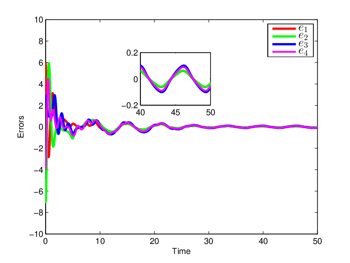
Figure 2: Tracking errors of all followers for t∈[0,50]t\in[0,50],

σ¯=0.06\bar{\sigma}=0.06, β=3\beta=3, α=0.4\alpha=0.4 and δ=0.001.\delta=0.001.

Refer to caption
Figure 3: Tracking errors of all followers for t∈[0,50]t\in[0,50],

σ¯=0.06\bar{\sigma}=0.06, β=3\beta=3, α=0.4\alpha=0.4 and δ=0.0001.\delta=0.0001.

Table 1: Event-triggered numbers of all agents.
Design parameters Time Triggering numbers for each agent
Agent 1 Agent 2 Agent 3 Agent 4
σ¯=0.06\bar{\sigma}=0.06, α=0.4\alpha=0.4 0-5s 59 71 104 110
β=1\beta=1, δ=0.0001\delta=0.0001
σ¯=0.06\bar{\sigma}=0.06, α=0.4\alpha=0.4 0-5s 50 59 86 84
β=3\beta=3, δ=0.0001\delta=0.0001
σ¯=0.06\bar{\sigma}=0.06, α=0.4\alpha=0.4 45-50s 128 133 176 137
β=3\beta=3, δ=0.0001\delta=0.0001
σ¯=0.06\bar{\sigma}=0.06, α=0.4\alpha=0.4 45-50s 38 40 72 64
β=3\beta=3, δ=0.001\delta=0.001

Simulation is performed with the unknown parameters w1=[0.4,−0.3,0.6,−0.7w_{1}=[0.4,-0.3,0.6,-0.7, 0.5,0.8,−0.2,−0.4]T0.5,0.8,-0.2,-0.4]^{T}, w2=[−0.3,0.2,0.5,−0.8,0.4,0.7w_{2}=[-0.3,0.2,0.5,-0.8,0.4,0.7, −0.1,−0.3]T-0.1,-0.3]^{T}, w3=[−0.6,−0.4,0.7,−0.8,0.4,0.2,−0.5w_{3}=[-0.6,-0.4,0.7,-0.8,0.4,0.2,-0.5, 0.1]T0.1]^{T}, w4=[0.3w_{4}=[0.3, −0.4,0.5,−0.6,0.3,0.7,−0.4,0.2]T-0.4,0.5,-0.6,0.3,0.7,-0.4,0.2]^{T} and the initial conditions z1​(0)=2,z2​(0)=4,z3​(0)=2,z4​(0)=1z_{1}(0)=2,~z_{2}(0)=4,~z_{3}(0)=2,~z_{4}(0)=1, ξ1​(0)=[7,−5]T,ξ2​(0)=[−6,−3]T\xi_{1}(0)=[7,-5]^{T},~\xi_{2}(0)=[-6,-3]^{T}, ξ3​(0)=[4,−3]T,ξ4​(0)=[−3,4]T,v⁡(0)=[1,0]T\xi_{3}(0)=[4,-3]^{T},~\xi_{4}(0)=[-3,4]^{T},v(0)=[1,0]^{T}, η1​(0)=[−3,1]T,η2​(0)=[3,−2]T\eta_{1}(0)=[-3,1]^{T},~\eta_{2}(0)=[3,-2]^{T}, η3​(0)=[2,−1]T,η4​(0)=[2,−1]T\eta_{3}(0)=[2,-1]^{T},~\eta_{4}(0)=[2,-1]^{T}, ζ1​(0)=[2,−5]T,ζ2​(0)=[2,3]T\zeta_{1}(0)=[2,-5]^{T},~\zeta_{2}(0)=[2,3]^{T}, ζ3​(0)=[3,−4]T,ζ4​(0)=[2,−5]T\zeta_{3}(0)=[3,-4]^{T},~\zeta_{4}(0)=[2,-5]^{T}.

Figures 2 and 3 show that, for i=1,2,3,4i=1,2,3,4, the tracking errors of all followers satisfy limt→∞|ei​(t)|≤0.5\lim_{t\rightarrow\infty}|e_{i}(t)|\leq 0.5 for δ=0.001\delta=0.001 and limt→∞|ei​(t)|≤0.2\lim_{t\rightarrow\infty}|e_{i}(t)|\leq 0.2 for δ=0.0001\delta=0.0001. It can be seen that the larger δ\delta leads to the larger tracking errors during the steady stage. Table 1 shows the event-triggered numbers of all followers. It can be seen that the larger β\beta leads to the less triggering numbers during the initial stage, and the larger δ\delta leads to the less triggering numbers during the steady stage.

6 Conclusion

In this paper, we have studied the cooperative robust practical output regulation problem for a class of linear minimum-phase multi-agent systems. By designing a distributed output feedback control law and a distributed output-based event-triggered mechanism, we have solved our problem and proved that the Zeno behavior can be prevented even if the neighbor-based measurement output is equal to zero. As we have revealed in Remark 2.3 that our event-triggered mechanism relies on the continuous-time output information from neighboring agents, thus costing communication resources. It is interesting to further consider how to design novel triggering mechanisms that avoid continuous communication by appropriate samplings.

Acknowledgment

The authors would like to thank the associate editor and the reviewers for their valuable comments and constructive suggestions.

References

  • [1] Abdelrahim, M., Postoyan, R., Daafouz, J., and Nesic, D. (2016). Stabilization of nonlinear systems using event-triggered output feedback controllers. IEEE Transactions on Automatic Control, 61(9), 2682–2687.
  • [2] Cheng, Y., and Ugrinovskii, V. (2016). Event-triggered leader-following tracking control for multivariable multi-agent systems. Automatica, 70, 204–210.
  • [3] Dimarogonas, D. V., Frazzoli, E., and Johansson, K. H. (2012). Distributed event-triggered control for multi-agent systems. IEEE Transactions on Automatic Control, 57(5), 1291–1297.
  • [4] Dolk, V. S., Borgers, D. P., and Heemels, W. P. M. H. (2017). Output-based and decentralized dynamic event-triggered control with guaranteed ℒp\mathcal{L}_{p}-gain performance and Zeno-freeness. IEEE Transactions on Automatic Control, 62(1), 34-49.
  • [5] Donkers, M. C. F., and Heemels, W. P. M. H. (2012). Output-based event-triggered control with guaranteed ℒ∞\mathcal{L}_{\infty}-gain and improved and decentralized event-triggering. IEEE Transactions on Automatic Control, 57(6), 1362–1376.
  • [6] Fan, Y., Feng, G., Wang, Y., and Song, C. (2013). Distributed event-triggered control of multi-agent systems with combinational measurements. Automatica, 49(2), 671–675.
  • [7] Girard, A. (2015). Dynamic triggering mechanisms for event-triggered control. IEEE Transactions on Automatic Control, 60(7), 1992–1997.
  • [8] Heemels, W. P. M. H., Johansson, K. H., and Tabuada, P. (2012). An introduction to event-triggered and self-triggered control. Proceedings of the 51st IEEE Conference on Decision and Control, Maul, Hawaii, USA, 3270–3285.
  • [9] Hu, J., and Hong, Y. (2007). Leader-following coordination of multi-agent systems with coupling time delays. Physica A: Statistical Mechanics and its Applications, 374(2), 853–863.
  • [10] Hu, W., and Liu, L. (2017). Cooperative output regulation of heterogeneous linear multi-agent systems by event-triggered control. IEEE Transactions on Cybernetics, 47(1), 105-116.
  • [11] Li, H., Liao, X., Huang, T., and Zhu, W. (2015). Event-triggering sampling based leader-following consensus in seconder-order multi-agent systems. IEEE Transactions on Automatic Control, 60(7), 1998–2003.
  • [12] Liu, T., and Jiang, Z. P. (2015) A small-gain approach to robust event-triggered control of nonlinear systems. IEEE Transactions on Automatic Control, 60(8), 2072–2085.
  • [13] Liu, W., and Huang, J. (2017). Robust practical output regulation for a class of uncertain linear minimum-phase systems by output-based event-triggered control. International Journal of Robust and Nonlinear Control, DOI: 10.1002/rnc.3815.
  • [14] Mu, N., Liao, X., and Huang, T. (2015). Leader-following consensus in second-order multiagent systems via event-triggered control with nonperiodic sampled data. IEEE Transactions on circuits and systems-II: express briefs, 62(10), 1007–1011.
  • [15] Nikiforov, V. O. (1998). Adaptive non-linear tracking with complete compensation of unknown disturbances. European Journal of Control, 4(2), 132–139.
  • [16] Postoyan, R., Tabuada, P., Nesic, D., and Anta, A. (2015). A framework for the event-triggered stabilization of nonlinear systems. IEEE Transactions on Automatic Control, 60(4), 982–996.
  • [17] Seyboth, G. S., Dimarogonas, D. V., and Johansson, K. H. (2013). Event-based broadcasting for multi-agent average consensus. Automatica, 49(1), 245–252.
  • [18] Su, Y., and Huang, J. (2014). Cooperative robust output regulation of a class of heterogeneous linear uncertain multi-agent systems. International Journal of Robust and Nonlinear Control, 24(17), 2819–2839.
  • [19] Tabuada, P. (2007). Event-triggered real-time scheduling of stabilizing control tasks. IEEE Transactions on Automatic Control, 52(9), 1680–1685.
  • [20] Tallapragada, P., and Chopra, N. (2013). On event triggered tracking for nonlinear systems. IEEE Transactions on Automatic Control, 58(9), 2343–2348.
  • [21] Wang, X., and Ni, W. (2012). Event-triggered output regulation for linear multi-agent systems. Proceedings of the 31st Chinese Control Conference, Hefei, China, 6177–6182.
  • [22] Wang, X., Ni, W., and Ma, Z. (2015). Distribtued event-triggered output regulation of multi-agent systems. International Journal of Control, 88(3), 640–652.
  • [23] Zhang, H., Feng, G., Yan, H., and Chen, Q. (2014). Observer-based output feedback event-triggered control for consensus of multi-agent systems. IEEE Transaction on Industrial Electronics, 61(9), 4885–4894.
  • [24] Zhu, W., Jiang, Z. P., and Feng, G. (2014). Event-based consensus of multi-agent systems with general linear models. Automatica, 50(2), 552–558.