Convex variational methods on graphs for multiclass segmentation of high-dimensional data and point clouds
Abstract
Graph-based variational methods have recently shown to be highly competitive for various classification problems of high-dimensional data, but are inherently difficult to handle from an optimization perspective. This paper proposes a convex relaxation for a certain set of graph-based multiclass data segmentation models involving a graph total variation term, region homogeneity terms, supervised information and certain constraints or penalty terms acting on the class sizes. Particular applications include semi-supervised classification of high-dimensional data and unsupervised segmentation of unstructured 3D point clouds. Theoretical analysis shows that the convex relaxation closely approximates the original NP-hard problems, and these observations are also confirmed experimentally. An efficient duality based algorithm is developed that handles all constraints on the labeling function implicitly. Experiments on semi-supervised classification indicate consistently higher accuracies than related non-convex approaches, and considerably so when the training data are not uniformly distributed among the data set. The accuracies are also highly competitive against a wide range of other established methods on three benchmark datasets. Experiments on 3D point clouds acquired by a LaDAR in outdoor scenes, demonstrate that the scenes can accurately be segmented into object classes such as vegetation, the ground plane and human-made structures.
Keywords:
variational methods graphical models convex optimization semi-supervised classification point cloud segmentation1 Introduction
The graphical framework has become a popular setting for classification [100, 101, 93, 8, 25, 102] and filtering [31, 34, 85, 63, 88, 89] of high-dimensional data. Some of the best performing classification algorithms are based on solving variational problems on graphs [82, 16, 10, 67, 44, 17, 15, 65, 40, 100, 25, 3, 86, 46]. In simple terms, these algorithms attempt to group the data points into classes in such a way that pairs of data points with different class memberships are as dissimilar as possible with respect to a certain feature. In order to avoid the computational complexity of working with fully connected graphs, approximations, such as those based on spectral graph theory [10, 67, 39] or nearest neighbors [33, 17, 65], are typically employed. For example, [10] and [67] employ spectral approaches along with the Nyström extension method [37] to efficiently calculate the eigendecomposition of a dense graph Laplacian. Works, such as [33, 40, 24, 99, 17, 65], use the “nearest neighbor” approach to sparsify the graph for computational efficiency. Variational problems on graphs have also become popular for processing of 3D point clouds [33, 61, 30, 46, 36, 55].
When the classification task is cast as the minimization of similarity of point pairs with different class membership, extra information is necessary to avoid the trivial global minimizer of value zero where all points are assigned to the same class. In semi-supervised classification methods, a small set of the data points are given as training data in advance, and their class memberships are imposed as hard constraints in the optimization problem. In unsupervised classification methods one typically enforces the sizes of each class not to deviate too far from each other, examples including the normalized cut [78] and Cheeger ratio cut problems [26].
Most of the computational methods for semi-supervised and unsupervised classification obtain the solution by computing the local minimizer of a non-convex energy functional. Examples of such algorithms are those based on phase fields [10] and the MBO scheme [67, 39, 66, 68]. PDEs on graphs for semi-supervised classification also include the Eikonal equation [30] and tug-of-war games related to the infinity-Laplacian equation [34]. Unsupervised problems with class size constraints are inherently the most difficult to handle from an optimization viewpoint, as the convex envelope of the problem has a trivial constant function as a minimizer [78, 82, 16]. Various ways of simplifying the energy landscape have been proposed [45, 17, 89]. Our recent work [65] showed that semi-supervised classification problems with two classes could be formulated in a completely convex framework and also presented efficient algorithms that could obtain global minimizers.
Image segmentation is a special classification problem where the objective is to assign each pixel to a region. Algorithms based on energy minimization are among the most successful image segmentation methods, and they have historically been divided into ‘region-based’ and ‘contour-based’.
Region-based methods attempt to find a partition of the image so that the pixels within each region as a whole are as similar as possible. Additionally, some regularity is imposed on the region boundaries to favor spatial grouping of the pixels. The similarity is usually measured in the statistical sense. In the simplest case, the pixels within each region should be similar to the mean intensity of each region, as proposed in the Chan-Vese [22] and Mumford-Shah [71] models. Contour-based methods [62, 90] instead seek the best suited locations of the region boundaries, typically at locations of large jumps in the image intensities, indicating the interface between two objects.
More recently, it has been shown that the combination of region and contour-based terms in the energy function can give qualitatively very good results [14, 40, 49], especially when non-local operators are used in the contour terms [40, 49, 30]. There now exists efficient algorithms for solving the resulting optimization problems that can avoid getting stuck in a local minimum, including both combinatorial optimization algorithms [11, 13, 53] and more recent convex continuous optimization algorithms [14, 98, 58, 75, 20, 7, 95, 97, 5]. The latter have shown to be advantageous in several aspects, such as the fact that they require less memory and have a greater potential for parallel implementation of graphics processing units (GPUs), but special care is needed in case of non-local variants of the differential operators (e.g. [76]).
Most of the current data segmentation methods [82, 16, 10, 67, 44, 17, 15, 65] can be viewed as ‘contour-based’, since they seek an optimal location of the boundaries of each region. Region-based variational image segmentation models with two classes were generalized to graphs for data segmentation in [59] and for 3D point cloud segmentation in [59, 36, 84] in a convex framework. The region terms could be constructed directly from the point geometry and/or be constructed from a color vector defined at the points. Concrete examples of the latter were used for experiments on point cloud segmentation. Region terms have also been proposed in the context of Markov Random Fields for 3D point cloud segmentation [2, 72, 87], where the weights were learned from training data using associate Markov networks. The independent preprint [94] proposed to use region terms for multiclass semi-supervised classification in a convex manner, where the region terms were inferred from the supervised points by diffusion.
Contributions
This paper proposes a convex relaxation and an efficient algorithmic optimization framework for a general set of graph based data classification problems that exhibits non-trivial global minimizers. It extends the convex approach for semi-supervised classification with two classes given in our previous work [65] to a much broader range of problems, including multiple classes, novel and more practically useful incorporation of class size information, and a novel unsupervised segmentation model for 3D point clouds acquired by a LaDAR.
The same basic relaxation for semi-supervised classification also appeared in the independent preprint [94]. The most major distinctions of this work compared to the preprint [94] are: we also incorporate class size information in the convex framework; we give a mathematical and experimental analysis of the close relation between the convex relaxed and original problems; we propose a different duality based ‘max-flow’ inspired algorithm; we incorporate information of the supervised points in a different way; and we consider unsupervised segmentation of 3D point clouds.
The contributions can be summarized more specifically as follows:
- •
We specify a general set of classification problems that are suitable for being approximated in a convex manner. The general set of problems involves minimization of a multiclass graph cut term together with supervised constraints, region homogeneity terms and novel constraints or penalty terms acting on the class sizes. Special cases include semi-supervised classification of high-dimensional data and unsupervised segmentation of 3D point clouds.
- •
A convex relaxation is proposed for the general set of problems and its approximation properties are analyzed thoroughly in theory and experiments. This extends the work on multiregion image segmentation [98, 58, 7] to data clustering on graphs, and to cases where there are constraints or penalty terms acting on the class sizes. Since either the introduction of multiple classes or size constraints causes the general problem to become NP-hard, the relaxation can (probably) not be proven to be exact. Instead, conditions are derived for when an exact global minimizer can be obtained from a dual solution of the relaxed problem. The strongest conditions are derived in case there are no constraints on the class sizes, but the theoretical results in both cases show that very close approximations are expected. These theoretical results also agree well with experimental observations.
- •
The convex relaxed problems are formulated as equivalent dual problems that are structurally similar to the ‘max-flow’ problem over the graph. This extends our work [65] to multiple classes and the work on image segmentation proposed in [96] to data clustering on graphs. We use a conceptually different proof than [65, 96], which relates ‘max-flow’ with another more direct dual formulation of the problem. Furthermore, it is shown that also the size constraints and penalty term can be incorporated naturally in the max-flow problem by modifying the flow conservation condition, such that there should be a constant flow excess at each node.
- •
As in our previous work [65, 96], an augmented Lagrangian algorithm is developed based on the new ‘max-flow’ dual formulations of the problems. A key advantage compared to related primal-dual algorithms [21] in imaging, such as the one considered in the preprint [94], is that all constraints on the labeling function are handled implicitly. This includes constraints on the class sizes, which are dealt with by separate dual variables indicating the flow excess at the nodes. Consequently, projections onto the constraint set of the labeling function, which tend to decrease the accuracy and put strict restrictions on the step sizes, are avoided.
- •
We propose an unsupervised segmentation model for unstructured 3D point clouds aquired by a LaDAR within the general framework. It extends the models of [59, 36, 84] to multiple classes and gives concrete examples of region terms constructed purely based on geometrical information of the unlabeled points, in order to distinguish classes such as vegetation, the ground plane and human-made structures in an outdoor scene. We also propose a graph total variation term that favors alignment of the region boundaries along “edges” indicated by discontinuities in the normal vectors or the depth coordinate. In contrast to [2, 72, 87, 42], our model does not rely on any training data.
- •
Extensive experimental evaluations on
semi-supervised classification indicate consistently higher accuracies than related local minimization approaches, and considerably so when the training data are not uniformly distributed among the data set. The accuracies are also highly competitive against a wide range of other established methods on three benchmark datasets. The accuracies can be improved further if an estimate of the approximate class sizes are given in advance. Experiments on 3D point clouds acquired by a LaDAR in outdoor scenes demonstrate that the scenes can accurately be segmented into object classes such as vegetation, the ground plane and regular structures. The experiments also demonstrate fast and highly accurate convergence of the algorithms, and show that the approximation difference between the convex and original problems vanishes or becomes extremely low in practice.
Organization
This paper starts by formulating the general set of problems mathematically in Section 2. Section 3 formulates a convex relaxation of the general problem and analyzes the quality of the relaxation from a dual perspective. Section 4 reformulates the dual problem as a ‘max-flow’ type of problem and derives an efficient algorithm. Applications to semi-supervised classification of high-dimensional data are presented in Section 5.1, and applications to segmentation of unstructured 3D point clouds are described in Section 5.2, including specific constructions of each term in the general model. Section 5 also presents a detailed experimental evaluation for both applications.
2 Data segmentation as energy minimization over a graph
Assume we are given data points in . In order to formulate the segmentation of the data points as a minimization problem, the points are first organized in an undirected graph. Each data point is represented by a node in the graph. The edges in the graph, denoted by , consist of pairs of data points. Weights on the edges measure the similarity between data points and . A high value of indicates that and are similar and a low value indicates that they are dissimilar. A popular choice for the weight function is the Gaussian
| (1) |
where is the distance, in some sense, between and . For example, the distance between two 3D points and is naturally their Euclidean distance. In order to reduce the computational burden of working with fully connected graphs, one often only considers the set of edges where is largest. For instance, edges may be constructed between each vertex in and its nearest neighbors. More formally, for each , one constructs an edge for the points with the shortest distance to . Such a graph can be constructed efficiently by using kd-trees in time [9, 47]. Note that the number of edges incident to some nodes in the resulting graph may be larger than , as illustrated in Figure 2 where , due to symmetry of the undirected graph. The construction of the graph itself provides a basic segmentation of the nodes, for instance in Figure 2, it can be observed that the graph contains 3 different connected components. This fact has been exploited in basic graph based classification methods [1].
In several recent works, the classification problem has been formulated as finding an optimal partition of the nodes in the graph . The most basic objective function can be formulated as
| (2) | ||||
| s.t. | (3) |
where the constraint (3) imposes that there should be no vacuum or overlap between the subsets . If , then (2) is the so-called “graph cut” [69]. The motivation behind the model (2) is to group the vertices into classes in such a way that pairs of vertices with different class memberships are as dissimilar as possible, indicated by a low value of .
2.1 Size constraints and supervised constraints
Extra assumptions are necessary to avoid the trivial global minimizer of (2), where for some and for all . There are two common ways to incorporate extra assumptions. In semi-supervised classification problems, the class membership of a small set of the data points is given as training data in advance by the constraints
| (4) |
where is the set of “training” points known to belong to class . For notational convenience, the set of all class indices is denoted by in the rest of this paper.
In unsupervised classification problems, one usually assumes that the regions should have approximately equal sizes. The simplest way to achieve this is to impose that each class should have a given size :
| (5) |
where . We focus on the case that the norm is the number of nodes in for simplicity. As an alternative, could be the sum of degrees of each node in , where the degree of a node is the number of edges incident to that node. If size constraints are introduced, the problem cannot generally be solved exactly due to NP-hardness. This will be discussed in more detail in Section 3.
Usually, a more flexible option is preferred of modifying the energy function such that partitions of equal sizes have lower energy. In case of two classes, the energy (2) becomes , where and . Several different ways of normalizing the energy by the class sizes have been proposed, which can be summarized as follows
| (6) |
The expression on the left is called the ratio cut in case of the norm and the normalized cut in case of . The expression on the right is called the Cheeger-ratio cut with the norm .
2.2 New flexible constraint and penalty term on class sizes
In this paper, we aim to provide a broader set of constraints and penalty terms acting on the class sizes that can be handled in a completely convex manner. They are designed to achieve the same net result as the ratio energies (6) of promoting classes of equal sizes, but in a completely convex way. They can also promote any other size relations between the class sizes. We will consider flexible size constraints of the form
| (7) |
where is an upper bound on the size of class and is a lower bound. Such types of constraints have previously been proposed for image segmentation in [52]. In case one only knows an estimate of the expected class sizes, such constraints can be used to enforce the sizes to lie within some interval of those estimates. To be well defined, it is obviously required that and . Note that if , then (7) becomes equivalent to (5).
To avoid imposing absolute upper and lower bounds on the class sizes, we also propose appending a piecewise-linear penalty term to the energy function (2), defined as
| (8) |
An illustration of is given in Figure 1. In the limit as , the penalty term becomes an equivalent representation of the hard constraints (7). Note that quadratic or higher order penalty terms, although they are convex, are not well suited for the convex relaxation, because they tend to encourage non-binary values of the labeling functions. In fact, we believe the set of constraints and penalty terms given here is complete when it comes to being suited for completely convex relaxations.
One major contribution of this paper is an efficient algorithmic framework that handles size constraints of the form (7) and the penalty term (8) naturally, with almost no additional computational efforts.
 |
2.3 Region homogeneity terms
The classification problem (2) involves the minimization of an energy on the boundary of the classes. The energy is minimized if the data points on each side of the boundary are as dissimilar as possible. These classification models are therefore similar to edge-based image segmentation models, which align the boundary of the regions along edges in the image where the intensity changes sharply. By contrast, region-based image segmentation models, such as the “Chan-Vese” model, use region homogeneity terms that measure how well each pixel fits with each region, in the energy function.
 |
A graph extension of variational segmentation problems with two classes was formulated in [59, 61, 36, 84], using a non-local total variation term together with a region term promoting homogeneity of a vertex function. The vertex function could be constructed directly from point geometry and/or from external information such as a color vector defined at each point. We extend the general problem to multiple classes and optional constraints as follows:
| (9) | ||||
| s.t. |
under optional supervised constraints (4) and/or size constraints (7)/penalty term (8). In [59, 61, 36, 84] the region terms were defined in terms of a general vertex function , which could depend on a color vector or the point geometry. Experimental results on point clouds were shown in case was a color vector defined at each point. In this work, we will give concrete constructions of for point cloud segmentation purely based on the geometry of the 3D points themselves. For example, the eigenvalues and eigenvectors obtained from a local PCA around each point carry useful information for describing the homogeneity within each class. Concrete examples are given in Section 5.2. An illustrative example is given in Figure 2, where each node is a 2D point and the region terms have been constructed to distinguish points with different statistical relations to their neighboring points.
The independent preprint [94], proposed to use region terms in the energy function for semi-supervised classification and the authors proposed a region term that was inferred from the supervised points by diffusion. In contrast, the region terms in this work do not rely on any supervised points, but are as mentioned only specified and demonstrated for the application of 3D point cloud segmentation.
3 Convex relaxation of minimization problem and analysis based on duality
In this section, the classification problems are formulated as optimization problems in terms of binary functions instead of sets. The binary representations are used to derive convex relaxations. First, some essential mathematical concepts are introduced, such as various differential operators on graphs. These concepts are used extensively to formulate the binary and convex problems and the algorithms.
3.1 Differential operators on graphs
Our definitions of operators on graphs are based on the theory in [43, 33, 91]. More information is found in these papers.
Consider two Hilbert spaces, and , which are associated with the sets of vertices and edges, respectively, and the following inner products and norms:
| (10) |
for some and . Above is the degree of node (it’s number of incident nodes) and is the weighting function.
From these definitions, we can define the gradient operator and the Dirichlet energy as
| (11) |
| (12) |
We use the equation to define the divergence:
| (13) |
where we have exploited symmetry of the undirected graph in the derivation of the operator.
Using divergence, a family of total variations can now be defined:
| (14) |
The definition of a family of graph Laplacians is:
| (15) |
3.2 Binary formulation of energy minimization problem
A partition of satisfying the no vacuum and overlap constraint
| (16) |
can be described by a binary vector function defined as
| (17) |
In other words, if and only if , where is the unit normal vector which is at the component and for all other components. The no vacuum and overlap constraint (16) can be expressed in terms of as
| (18) |
Moreover, note that the minimization term of (2) can be naturally related to total variation (14) for . In fact,
| (19) |
This connection between the two terms was used in several recent works to derive, utilizing the graphical framework, efficient unsupervised algorithms for clustering. For example, [16, 89] formulate rigorous convergence results for two methods that solve the relaxed Cheeger cut problem, using non-local total variation. Moreover, [82] provides a continuous relaxation of the Cheeger cut problem, and derives an efficient algorithm for finding good cuts. The authors of [82] relate the Cheeger cut to total variation, and then present a split-Bregman approach of solving the problem. In [88] the continuum limit of total variation on point clouds was derived.
The general set of problems (9) can now be formulated in terms of as
| (20) |
where
| (21) |
is the set of binary functions indicating the partition. The superscript stands for “primal”. The optional size constraints (7), can be imposed in the terms of as
where . The size penalty term (8) can be imposed by appending the energy function (20) with the term .
In case of semi-supervised classification, takes the form of
| (22) |
where is a binary function taking the value of in and elsewhere, and is a function that takes on a large constant value on supervised points and zero elsewhere. If is chosen sufficiently large, it can be guaranteed that the solution satisfies the supervised constraints. The algorithm to be presented in this work does not require the selection of an appropriate value for the parameter , as the ideal case where can be handled naturally without introducing numerical instabilities.
Region homogeneity terms can be imposed by setting . More generally, region homogeneity terms and supervised data points can be combined by setting
| (23) |
The total variation term is defined as in (14) with .
If the number of supervised points is very low and there is no additional region term, the global minimizer of (20) may become the trivial solution where for one of the classes, say , everywhere, and for the other classes for supervised points of class and elsewhere. The threshold tends to occur around less than of the points. As in our previous work [65], this problem can be countered by increasing the number of edges incident to supervised points in comparison to other points. Doing so will increase the cost of the trivial solution without significantly influencing the desired global minimizer. An alternative, proposed in the preprint [94], is to create region terms in a pre-processing step by diffusing information of the supervised points into their neighbors.
3.3 Convex relaxation of energy minimization problem
Due to the binary constraints (21), the problem (20) is non-convex. As in several recent works on variational image segmentation [98, 58, 60, 7, 18, 77] and MRF optimization [51, 12, 54, 2], we replace the indicator constraint set (21) by the convex unit simplex
| (24) |
Hence, we are interested in solving the following convex relaxed problem
| (25) |
under optional size constraints (7) or penalty term (8). In case and no size constraints, the relaxation is exact, as proven for image segmentation in [80, 23] and classification problems on graphs in [59, 65]. In case , the problem becomes equivalent to a multiway cut problem, which is known to be NP-hard [28]. In case size constraints are imposed, the problem becomes NP-hard even when , as it becomes equivalent to a knapsack problem [64] in the special case of no TV term.
In this paper we are interested in using the convex relaxation (25) to solve the original problem approximately. Under certain conditions, the convex relaxation gives an exact global minimizer of the original problem. For instance, it can be straight forwardly shown that
Proposition 1
Proof.
If the computed solution of (25) is not completely binary, one way to obtain an approximate binary solution that exactly indicates the class membership of each point, is to select the binary function as the nearest vertex in the unit simplex by the threshold
| (26) |
As an alternative to the threshold scheme (26), binary solutions of the convex relaxation (25) can also be obtained from a dual solution of (25), which has a more solid theoretical justification if some conditions are fulfilled. The dual problem also gives insight into why the convex relaxation is expected to closely approximate the original problem. This is the topic of the next section.
3.4 Analysis of convex relaxation through a dual formulation
We will now derive theoretical results which indicate that the multiclass problem (20) is closely approximated by the convex relaxation (25). The following results extend those given in [7] from image domains to graphs. In contrast to [7], we also incorporate size constraints or penalty terms in the analysis. In fact, the strongest results given near the end of the section are only valid for problems without such size constraints/terms. This observation agrees well with our experiments, although in both cases very close approximations are obtained.
We start by deriving an equivalent dual formulation of (25). Note that this dual problem is different from the “max-flow” type dual problem on graphs proposed in our previous work [65] in case of two classes. Its main purpose is theoretical analysis, not algorithmic development. In fact, its relation to flow maximization will be the subject of the next section. Dual formulations on graphs have also been proposed in [46] for variational multiscale decomposition of graph signals.
Theorem 3.1
The convex relaxed problem (25) can equivalently be formulated as the dual problem
| (27) |
subject to
| (28) | ||||
| (29) |
where the above set of infinity norm spheres is defined as
| (30) |
No size information is incorporated by choosing . The size penalty term (8) is incorporated by choosing . Size constraints (7) are incorporated by choosing .
Proof.
By using the definition of total variation (14), the problem (25) with size penalty term (8) can be expressed in primal-dual form as
| (31) |
where is defined in (30). It will be shown that the size constraints (7) or penalty term (8) can be implicitly incorporated by introducing the dual variables , as
| (32) |
The primal-dual problem (32) satisfies all the conditions of the mini-max theorem (see e.g. Chapter 6, Proposition 2.4 of [32]). The constraint sets for and are compact and convex, and the energy function is convex l.s.c. for fixed and concave u.s.c. for fixed . This implies the existence of at least one primal-dual solution (saddle point) of finite energy value.
For a given , the terms involving and can be rearranged as
Consider the above three choices for . In case the class sizes do not contribute to the energy. In case the two above terms summed together is exactly equal to the size penalty term . In case , the constraint set on is no longer compact, but we can apply Sion’s generalization of the mini-max theorem [79], which allows either the primal or dual constraint set to be non-compact. It follows that if the size constraints (7) are not satisfied, the energy would be infinite, contradicting existence of a primal-dual solution.
From the mini-max theorems, it also follows that the inf and sup operators can be interchanged as follows
| (37) |
For notational convenience, we denote the unit simplex pointwise as
| (38) |
For an arbitrary vector , observe that
| (39) |
Therefore, the inner minimization of (37) can be solved analytically at each position , and we obtain the dual problem
∎
Assuming a solution of the dual problem has been obtained, the following theorem characterizes the corresponding primal variable
Theorem 3.2
There exists a maximizer to the dual problem (27). At the point , let be the set of indices such that
| (40) |
There exists a solution to the primal problem (25) such that is a primal-dual pair. At the point , must satisfy
| (41) |
If the minimizer (40) is unique at the point , then the corresponding primal solution at the point must be valued
| (42) |
If the minimizer (40) is unique at every point , then the corresponding primal solution , given by the formula (42), is an exact global binary minimizer of the original non-convex problem (20).
Proof.
Since all conditions of the mini-max theorem [32, 79] are satisfied (c.f. proof of Theorem 3.1), there must exist a maximizer of the dual problem (27) and a minimizer of the primal problem (25) such that is a solution of the primal-dual problem (31) (see e.g. [32]). For arbitrary vectors and , it must hold that . Therefore, at the point , must satisfy
otherwise the primal-dual energy would exceed the dual energy, contradicting strong duality. The above expression can be further decomposed as follows
Since
for all , the above can only be true provided
and for .
It can also be shown that an exact binary primal solution exists if there are two non-unique minimal components to the vector
but this result only holds in case there are no constraints acting on the class sizes.
Theorem 3.3
Assume that is a maximizer of the dual problem (27) with , i.e. no class size constraints. If (40) has at most two minimal components for all , then there exists a corresponding binary primal solution to the convex relaxed primal problem (25), which is a global minimizer of the original non-convex problem (20).
If the vector has three or more minimal components, it cannot in general be expected that a corresponding binary primal solution exists, reflecting that one can probably not obtain an exact solution to the NP-hard problem (20) in general by a convex relaxation. Experiments indicate that this very rarely, if ever, happens in practice for the classification problem (20).
As an alternative thresholding scheme, can be selected based on the formula (42) after a dual solution to the convex relaxation has been obtained. If there are multiple minimal components to the vector , one can select to be one for an arbitrary one of those indices, just as for the ordinary thresholding scheme (26). Experiments will demonstrate and compare both schemes in Section 5.
4 ‘Max-flow’ formulation of dual problem and algorithm
A drawback of the dual model (27) is the non-smoothness of the objective function, which is also a drawback of the original primal formulation of the convex relaxation. This section reformulates the dual model in a structurally similar way to a max-flow problem, which is smooth and facilitates the development of a very efficient algorithm based on the augmented Lagrangian theory.
The resulting dual problem can be seen as a multiclass variant of the max-flow model proposed in our work [65] for two classes, and a graph analogue of the max-flow model given for image domains in [96]. Note that our derivations differ conceptually from [96, 65], because we directly utilize the dual problem derived in the last section. Furthermore, the new flexible size constraint (7) and penalty term (8) are incorporated naturally in the max-flow problem by a modified flow conservation condition, which indicates that there should be a constant flow excess at each node. The amount of flow excess is expressed with a few additional optimization variables in the algorithm, and they can optimized over with very little additional computational cost.
4.1 ‘Max-flow’ reformulation dual problem
We now derive alternative dual and primal-dual formulations of the convex relaxed problem that are more beneficial for computations. The algorithm will be presented in the next section.
Proposition 2
The dual problem (27) can equivalently be formulated as the dual ‘max-flow’ problem:
| (43) |
subject to, for all ,
| (44) | ||||
| (45) | ||||
| (46) | ||||
| (47) |
Proof.
By introducing the auxiliary variable , the dual problem (27) can be reformulated as follows
| subject to, for all , | |||
| subject to, for all , | ||||
| (48) | ||||
By adding another set of auxiliary variables , , the constraints (48) can be formulated as
| (49) | ||||
for all and all . Rearranging the terms in constraint (49), and using the definition of the infinity norm (10), leads to the ‘max-flow’ model (43) subject to (44)-(47). ∎
Problem (43) with constraints (44)-(47) is structurally similar to a max-flow problem over copies of the graph , , where for . The aim of the max-flow problem is to maximize the flow from a source vertex to a sink vertex under flow capacity at each edge and flow conservation at each node. The variable can be regarded as the flow on the edges from the source to the vertex in each of the subgraphs , which have unbounded capacities. The variables and can be regarded as the flow and capacity on the edge from vertex in the subgraph to the sink. Constraint (49) is the flow conservation condition. Observe that in case of size constraints/terms, instead of being conserved, there should be a constant excess flow for each node in the subgraph . The objective function (43) is a measure of the total amount of flow in the graph.
Utilizing results from Section 3.4, we now show that the convex relaxation (25) is the equivalent dual problem to the max-flow problem (43).
Theorem 4.1
Proof.
The equivalence between the primal-dual problem (50) and the max-flow problem (43) follows directly as is an unconstrained Lagrange multiplier for the flow conservation constraint (49). Existence of the Lagrange multipliers follows as: 1) (43) is upper bounded, since it is equivalent to (27), which by Theorem 3.2 admits a solution; 2) the constraints (46) are linear, and hence differentiable.
The equivalence between the primal-dual problem (50), the max-flow problem (43) and the convex relaxed problem (25) now follows: By Proposition 2 the ‘max-flow’ problem (43) is equivalent to the dual problem (27). By Theorem 3.1, the dual problem (27) is equivalent to the convex relaxed problem (25) with size constraints (7) if , size penalty term (8) if and no size constraints if .
∎
Note an important distinction between the primal-dual problem (50) and the primal-dual problem (37) derived in the last section: The primal variable is unconstrained in (50). The simplex constraint is handled implicitly. It may not seem obvious from the proof how the constraints on are encoded in the primal-dual problem, therefore we give some further insights: For a given primal variable , the maximization with respect to of the primal-dual problem (50) at the point can be rearranged as
If does not satisfy the sum to one constraint at , then the primal-dual energy would be infinite, contradicting boundedness from above. In a similar manner, the optimization with respect to can be expressed as
which would be infinite if does not satisfy the non-negativity constraints. If , the indicator function of class , the value would be , which is indeed the pointwise cost of assigning to class .
4.2 Augmented Lagrangian max-flow algorithm
This section derives an efficient algorithm, which exploits the fact all constraints on are handled implicitly in the primal-dual problem (50). The algorithm is based on the augmented Lagrangian theory, where is updated as a Lagrange multiplier by a gradient descent step each iteration. Since no subsequent projection of is necessary, the algorithm tolerates a wide range of step sizes and converges with high accuracy. The advantages of related ‘max-flow’ algorithms for ordinary 2D imaging problems over e.g. Arrow-Hurwicz type primal-dual algorithms have been demonstrated in [6, 97].
From the primal-dual problem (50), we first construct the augmented Lagrangian functional:
| (55) |
An augmented Lagrangian algorithm for minimizing the above functional is given below, which involves alternatively maximizing for the dual variables and then updating the Lagrange multiplier .
Note that if there are no constraints on the class sizes, , then for every iteration . The algorithm can in this case be simplified by setting for all and ignoring all steps involving and .
Algorithm 1
Initialize , , , , and . For until convergence:
-
Optimize flow, for
(56) where is fixed.
-
Optimize source flow
(57) where is fixed.
-
Optimize sink flow , for ,
(58) where is fixed.
-
Optimize , for ,
(59) where is fixed.
-
Optimize , for ,
(60) where is fixed.
-
Update , for
The optimization problem (56) can be solved by a few steps of the projected gradient method as follows:
| (61) |
Above, is a projection operator which is defined as
| (62) |
where sgn is the sign function. There are extended convergence theories for the augmented Lagrangian method in the case when one of the subproblems is solved inexactly, see e.g. [35, 41]. In our experience, one gradient ascent iteration leads to the fastest overall speed of convergence.
The subproblems (57) and (58) can be solved by
| (63) |
| (64) |
Consider now the subproblems (59) and (60). In case no constraints are given on and , the maximizers over the sum of the concave quadratic terms can be computed as the average of the maximizers to each individual term as
respectively for and . Since the objective function is concave, and the maximization variable is just a constant, an exact solution to the constrained maximization problem can now be obtained by a projection onto that constraint as follows
| (65) | ||||
| (66) |
Algorithm 1 is suitable for parallel implementation on GPU, since the subproblems at each substep can be solved pointwise independently of each other using simple floating point arithmetics. The update formula (61) for , which only requires access to the values of neighboring nodes at the previous iterate. As discussed in Section 2, the number of neighbors may vary for nodes across the graph, therefore special considerations should be taken when declaring memory. We have implemented the algorithm on CPU for experimental evaluation for simplicity.
5 Applications and experiments
We now focus on specific applications of the convex framework. Experimental results on semi-supervised classification of high-dimensional data are presented in Section 5.1. Section 5.2 proposes specific terms in the general model (9) for segmentation of unstructured 3D point clouds, and presents experimental results on LaDAR data acquired in outdoor scenes. In both cases we give a thorough examination of accuracy of the results, tightness of the convex relaxations, and convergence properties of the algorithms.
A useful quality measure of the convex relaxation is to what extent the computed solution is binary. Proposition 1 indicates that if the computed solution is completely binary, it is also an exact global minimizer to the original non-convex problem. Let be a thresholding of in the sense that each row of is modified to be the closest vertex in the unit simplex according to the scheme (26). As a quality measure of the solution at each iteration of Algorithm 1, we calculate the average difference between and its thresholded version as follows:
| (67) |
where is the number of nodes, and is the number of classes. We call the “binary difference” of at iteration . Naturally, we want to become as low as possible as the algorithm converges.
5.1 Semi-supervised classification results
In this section, we describe the supervised classification results, using the algorithm with and without the size constraints (5), (7) or penalty term (8).
We compare the accuracy of the results with respect to the ground truth. The results are also compared against other local minimization approaches in terms of the final total variation energies:
where is the number of classes. A lower value of is better. The energy contribution from the fidelity term is ignored because the solution satisfies the supervised constraints by construction, thus giving zero contribution from those terms.
To compute the weights for the data sets, we use the Zelnik-Manor and Perona weight function [74]. The function is defined as:
| (68) |
where is a distance measure between vertices and , and is the distance between vertex and its closest neighbor. If is not among the nearest neighbors of , then is set to 0. After the graph is computed, we symmetrize it by setting
Here, is a parameter to be chosen. The weight function will be defined more specifically for each application.
We run the minimization procedure until the following stopping criterion is satisfied:
where is the from the previous iteration, and the value of varies depending on the data set (anywhere from to ).
All experiments were performed on a 2.4 GHz Intel Core i2 Quad CPU. We initialize constant (in our case, the constant is set to 500) if is a supervised point of any class but class , and otherwise, for all . The variables , , , are initialized to zero for all . The variable is initialized to , where is the number of classes. We set .
In the following, we give details about the set up and results for each dataset, before we draw some general conclusions in the end.
5.1.1 MNIST
The MNIST data set [57], affiliated with the Courant Institute of New York University, consists of images of handwritten digits through . Some of the images in the database are shown in Figure 3. The objective is, of course, to assign the correct digit to each image; thus, this is a -class segmentation problem.
We construct the graph as follows; each image is a node on a graph, described by the feature vector of pixel intensity values in the image. These feature vectors are used to compute the weights for pairs of nodes. The weight matrix is computed using the Zelnik-Manor and Perona weight function (68) with local scaling using the closest neighbor. We note that preprocessing of the data is not needed to obtain an accurate classification; we do not perform any preprocessing. The parameter used was 0.05.

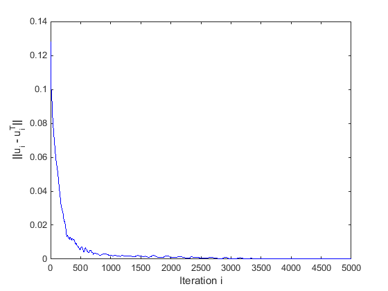
The average accuracy results over 100 different runs with randomly chosen supervised points are shown in Table 1 in case of no size constraints. We note that the new approaches reach consistently higher accuracies and lower energies than related local minimization approaches, and that incorporation of size information can improve the accuracies further. The computation times are highly efficient, but not quite as fast as MBO, which only uses 10 iteration to solve the problem in an approximate manner. The plots of the binary difference versus iteration, depicted in Figure 7, show that the binary difference converges to an extremely small number.


The results of the data set are visualized in Figure 4. For the visualization procedure, we use the first and the sixth eigenvector of the graph Laplacian. The dimension of each of the eigenvectors is , and each node of the data set is associated with a value of each of the vectors. One way to visualize a classification of a data set such as MNIST, which consists of a collection of images, is to plot the values of one eigenvector of the graph Laplacian versus another and use colors to differentiate classes in a given segmentation. In this case, the plots in Figure 4 graph the values of the first versus the sixth eigenvector (of the graph Laplacian) relating to the nodes of class 4 and 9 only. The blue and red region represents nodes of class 4 and 9, respectively. The green region represents misclassified points.
Moreover, we compare our results to those of other methods in Table 1, where our method’s name is written in bold. Note that algorithms such as linear and nonlinear classifiers, boosted stumps, support vector machines and both neural and convolution nets are all supervised learning approaches, which use around of the images as a training set ( of the data) and images for testing. However, we use only (or less) of our data as supervised training points, and obtain classification results that are either competitive or better than those of some of the best methods. Moreover, note that no preprocessing was performed on the data, as was needed for some of the methods we compare with; we worked with the raw data directly.
5.1.2 Three Moons Data Set
We created a synthetic data set, called the three moons data set, to test our method. The set is constructed as follows. First, consider three half circles in . The first two half top circles are unit circles with centers at and . The third half circle is a bottom half circle with radius of and center at . A thousand points from each of the three half circles are sampled and embedded in by adding Gaussian noise with standard deviation of to each of the components of each embedded point. The goal is to segment the circles, using a small number of supervised points from each class. Thus, this is a 3-class segmentation problem. The noise and the fact that the points are embedded in high-dimensional space make this difficult.
We construct the graph as follows; each point is a node on a graph, described by the feature vector consisting of the dimensions of the point. To compute the distance component of the weight function for pairs of nodes, we use these feature vectors. The weight matrix is computed using the Zelnik-Manor and Perona weight function (68) with local scaling using the nearest neighbor. The parameter was 0.1.


The results of the data set are visualized in Figure 5 and the accuracies are shown in Table 1. This is the only dataset where the proposed approach got lower accuracy than MBO. For this particular example, the global minimizer does not seem the best in terms of accuracy, which is a fault of the model rather than an optimization procedure.


5.1.3 COIL
We evaluated our performance on the benchmark COIL data set [73, 25] from the Columbia University Image Library. This is a set of color images of objects, taken at different angles. The red channel of each image was downsampled to pixels by averaging over blocks of pixels. Then, of the objects were randomly selected and then partitioned into six classes. Discarding images from each class leaves per class, giving a data set of data points and 6 classes.
We construct the graph as follows; each image is a node on a graph. We apply PCA to project each image onto 241 principal components; these components form the feature vectors. The vectors are used to calculate the distance component of the weight function. The weight matrix is computed using the Zelnik-Manor and Perona weight function (68) with local scaling using the nearest neighbor. The parameter used was 0.03.
Resulting accuracies are shown in Table 1, indicating that our method outperforms local minimization approaches and is comparable to or better than some of the other best existing methods. The results of the data set are visualized in Figure 6; the procedure used is similar to that of the MNIST data set visualization procedure. The plots in the figure graph the values of the first versus the third eigenvector of the graph Laplacian. The results of the classification are labeled by different colors.
5.1.4 Landsat Satellite data set
We also evaluated our performance on the Landsat Satellite data set, obtained from the UCI Machine Learning Repository [4]. This is a hyperspectral data set which is composed of sets of multi-spectral values of pixels in 3 3 neighborhoods in a satellite image; the portions of the electromagnetic spectrum covered include near-infrared. The goal is to predict the classification of the central pixel in each element of the data set. The six classes are red soil, cotton crop, grey soil, damp grey soil, soil with vegetation stubble and very damp grey soil. There are 6435 nodes in the data set.
We construct the graph as follows. The UCI website provides a -dimensional feature vector for each node. The feature vectors are used to calculate the distance component of the weight function. The weight matrix is computed using the Zelnik-Manor and Perona weight function (68) with local scaling using the nearest neighbor. The parameter c used was 0.3.
Table 1 includes comparison of our method to some of the best methods (most cited in [70]). One can see that our results are of higher accuracy. We now note that, except the GL and MBO algorithms, all other algorithms we compare the Landsat satellite data to are supervised learning methods, which use 80% of data for training and 20% for testing. Our method was able to outperform these algorithms while using a very small percentage of the data set (10%) as supervised points. Even with 5.6% supervised points it outperforms all but one of the aforementioned methods.
5.1.5 Non-uniform distribution of supervised points
In all previous experiments, the supervised points have been sampled randomly from all the datapoints. To test the algorithms in more challenging scenarios, we introduce some bias in the sampling of the supervised points, which is also a more realistic situation in practice. We used two different data sets for this test: the MNIST data set and the COIL data set.
In the case of the MNIST data set, we chose the supervised points non-randomly for digits and only. To obtain the non-randomness, we allowed a point to be chosen as supervised only if it had a particular range of values for the second eigenvector. This resulted in a biased distribution of the supervised points. The results for this experiment were the following: for the max flow algorithm, the overall accuracy was , while for digits and , it was . For comparison, the non-convex MBO algorithm [39] gave an accuracy of overall, but for digits and . The MBO method was also a bit more unstable in its accuracy with respect to different distributions of the supervised points. The max-flow algorithm was very stable, with a very small standard deviation for a set of accuracies for different supervised point distributions.
In the case of the COIL data set, we chose the supervised points non-randomly for classes and . The non-randomness was achieved in the same way as for the MNIST data set. The results were the following: the overall accuracy of the max-flow was , while for classes and , it was . The MBO algorithm [39] gave an accuracy of overall, but for classes and .
These results are summarized in Table 3 and are visualized in Figures 4 and 6 for MNIST and COIL data sets, respectively.


5.1.6 Experiments with size constraints and penalty term
The exact size constraints (5) could improve the accuracies if knowledge of the exact class sizes are available. However, it is not realistic to obtain the exact knowledge of the class sizes in practice, and this was the motivation behind developing the flexible constraints (7) or the penalty term (8). In order to simulate the case that only an estimate of the class sizes are known, we perturb the exact class sizes by a random number ranging between 1 and 20 of . The lower and upper bounds in (7) and (8) are centered around the perturbed class size, and the difference between them is chosen based on the uncertainty of the estimation, which we assume to be known. More specifically, denoting the exact class size , the perturbed class size is chosen as a random number in the interval . In experiments, we select as 1 , 10 and 20 of . The lower and upper bounds in the flexible size constraint (7) and the penalty term (8) are chosen as and . The parameter in the penalty term is set to for all datasets.
We run the algorithm for each choice of several times with different random selections of the perturbed class size each time. The average accuracies over all the runs for each choice of are shown in Table 3. The flexible size constraints or penalty term improve the accuracy compared to the case when no size information was given, shown in Table 1. Note that the accuracy improves also in cases of great uncertainty in the class size estimates (). The exact size constraints can be seen to not be suitable in case knowledge of the exact class sizes are not known, as imposing them significantly reduces the accuracies in those cases.
Note that some of the comparable algorithms, marked by *, use substantially more data for training ( at most and at smallest) than the proposed algorithm, see the main text for more information.
| Method | Accuracy |
|---|---|
| p-Laplacian [19] | 87.1% |
| multicut normalized 1-cut [45] | 87.64% |
| linear classifiers [56, 57] | 88% |
| Cheeger cuts [82] | 88.2% |
| boosted stumps* [50, 57] | 92.3-98.74% |
| transductive classification [83] | 92.6% |
| tree GL [38] | 93.0% |
| -nearest neighbors* [56, 57] | 95.0-97.17% |
| neural/conv. nets* [56, 27, 57] | 95.3-99.65% |
| nonlinear classifiers* [56, 57] | 96.4-96.7% |
| SVM* [56, 29] | 98.6-99.32% |
| GL [39] (3.57% supervised pts.) | 96.8% |
| MBO [39] (3.57% supervised pts.) | 96.91% |
| Proposed (3.57% supervised pts.) | 97.709% |
| Method | Accuracy |
|---|---|
| -nearest neighbors [81] | 83.5% |
| LapRLS [8, 81] | 87.8% |
| sGT [48, 81] | 89.9% |
| SQ-Loss-I [81] | 90.9% |
| MP [81] | 91.1% |
| GL [39] | 91.2% |
| MBO [39] | 91.46% |
| Proposed | 93.302% |
*-marked use of the data set for training, see main text for more information
| Method | Accuracy |
|---|---|
| SC-SVM* [70] | 65.15% |
| SH- SVM* [70] | 75.43% |
| S-LS* [70] ) | 65.88% |
| simplex boosting* [70] | 86.65% |
| S-LS rbf.* [70] | 90.15% |
| GL [39] (10% supervised pts.) | 87.62% |
| GL [39] (5.6% supervised pts.) | 87.05% |
| MBO [39] (10% supervised pts.) | 87.76% |
| MBO [39] (5.6% supervised pts.) | 87.25% |
| Proposed (10% supervised pts.) | 90.267% |
| Proposed (5.6% supervised pts.) | 88.621% |
| overall | classes 4 and 9 | |
|---|---|---|
| Proposed, MNIST | 97.734% | 96.85% |
| MBO, MNIST | 95.60% | 89.72% |
| overall | classes 2 and 6 | |
| Proposed, COIL | 92.69% | 90.89% |
| MBO, COIL | 83.90% | 77.24% |
MNIST, 3.57% supervised points
| max size perturbation () | |||
|---|---|---|---|
| flexible size constraints (7) | 97.761 | 97.725 | 97.716 |
| penalty term (8) | 97.755 | 97.739 | 97.722 |
| exact size constraints (5) | 96.139 | 70.820 | 63.660 |
| supervised points | |||
|---|---|---|---|
| max size perturbation () | |||
| flexible size constraints (7) | 99.374 | 98.829 | 98.750 |
| penalty term (8) | 99.368 | 98.789 | 98.718 |
| exact size constraints (5) | 99.108 | 72.685 | 66.627 |
| supervised points | |||
| max size perturbation () | |||
| flexible size constraints (7) | 97.833 | 97.738 | 97.160 |
| penalty term (8) | 97.848 | 97.793 | 97.406 |
| exact size constraints (5) | 97.706 | 68.956 | 66.872 |
| supervised points | |||
|---|---|---|---|
| max size perturbation () | |||
| flexible size constraints (7) | 93.403 | 93.535 | 93.527 |
| penalty term (8) | 93.360 | 93.418 | 93.325 |
| exact size constraints (5) | 92.990 | 59.936 | 55.624 |
| supervised points | |||
| max size perturbation () | |||
| flexible size constraints (7) | 90.428 | 90.892 | 90.730 |
| penalty term (8) | 89.957 | 90.967 | 90.712 |
| exact size constraints (5) | 89.931 | 55.152 | 54.674 |
| supervised points | |||
|---|---|---|---|
| max size perturbation () | |||
| flexible size constraints (7) | 90.504 | 90.397 | 90.344 |
| penalty term (8) | 90.479 | 90.371 | 90.347 |
| exact size constraints (5) | 87.773 | 67.687 | 65.757 |
| supervised points | |||
| max size perturbation () | |||
| flexible size constraints (7) | 89.024 | 89.022 | 88.848 |
| penalty term (8) | 89.025 | 89.018 | 88.987 |
| exact size constraints (5) | 86.327 | 60.904 | 51.276 |
| MBO [39] | GL [39] | Proposed | |
| MNIST | 15.4 | 153.1 | 42.5 |
| 3 moons | 3.7 | 3.9 | 2.7 |
| COIL | 1.18 | 1.19 | 1.4 |
| satellite | 16.4 | 23 | 16.5 |
| initial energy | final energy | final energy | |
|---|---|---|---|
| (MBO) [39] | proposed | ||
| MNIST | 225654 | 15196 | 12324 |
| 3 moons | 5982.79 | 433.19 | 420.24 |
| COIL | 1774.3 | 24.61 | 24.18 |
| satellite | 5116.9 | 221.87 | 214.95 |
5.1.7 Summary of experimental results
Experimental results on the benchmark datasets, shown in Table 1, indicate a consistently higher accuracy of the proposed convex algorithm than related local minimization approaches based on the MBO or Ginzburg-Landau scheme. The improvements are especially significant when the supervised points are not uniformly distributed among the dataset as shown in Table 3. On one synthetic dataset, “three moons”, the accuracy of the new algorithm was slightly worse, indicating that the global minimizer was not the best in terms of accuracy for this particular toy example. Table 5 shows that the new algorithm reaches the lowest energy on all of the experiments, further indicating that MBO and Ginzburg-Landau are not able to converge to the global minimum. Table 1 shows that the accuracies of the proposed algorithm are also highly competitive against a wide range of other established algorithms, even when substantially less training data than those algorithms are being used. Table 3 shows that that the flexible size constraints (7) and penalty term (8) can improve the accuracy, if a rough estimate of the approximate class sizes are given.
The binary difference (67), plotted on log-scale against the iteration count, is depicted for each experiment in Figure 7. For experiments without any size information, the average binary difference tends to less than , which is vanishingly low and more or less indicates that an exact global minimizer has been obtained. For experiments with size constraints or penalty terms, the binary difference also gets very low, although not as low. This indicates convergence to at least a very close approximation of the global minimizer. These observations agree well with the theoretical results in Section 3.4, where the strongest results were also obtained in case of no size information.
Note that a lot more iterations than necessary have been used in the binary difference plots. In practice, the algorithm reaches sufficient stability in 100-300 iterations. The CPU times, summerized in Table 4, indicate a fast convergence of the new algorithm, much faster than GL, although not quite as fast as the MBO scheme. It must be noted that MBO is an extremely fast front propagation algorithm that only uses a few (e.g. 10) iterations, but its accuracy is limited due to the large step sizes. A deeper discussion on the number of iterations needed to reach the exact solution after thresholding will be given at the end of the next section on point cloud segmentation.
5.2 Segmentation of 3D point clouds
The energy function (9) that combines region homogeneity terms and dissimilarity across region boundaries will be demonstrated for segmentation of unstructured 3D point clouds, where each point is a vertex in . Point clouds arise for instance through laser-based range imaging or multiple view scene reconstruction. The results of point cloud segmentation are easy to visualize and the choice of each term in the energy function will have a clear intuitive meaning that may be translated to other graph-based classification problems in the future. We focus especially on point clouds acquired through the concept of laser detection and ranging (LaDAR) in outdoor scenarios. A fundamental computer vision task is to segment such scenes into classes of similar objects. Roughly, some of the most common object classes in an outdoor scene are the ground plane, vegetation and human-made “objects” with a certain regular structure.
5.2.1 Construction of the energy function
We construct the graph by connecting each node to its k nearest neighbors (kNN) based on the Euclidian distance as described at the beginning of Section 2. In experiments, we set . We construct region terms that favor homogeneity of geometrical features based on a combination of point coordinates, normal vectors and variation of normal vectors. The construction is a concrete realization of the general region terms introduced in [59, 36, 84]. We also propose to use a contour term that favors alignment of the boundaries of the regions at “edges”, indicated by sharp discontinuities of the normal vectors. Our model can be seen as a point cloud analogue of variational models for traditional image segmentation, that combine region and edge based features in a single energy functional [14, 40, 49]. In contrast to the work [2, 72, 87] our model does not rely on training data.
Normal vectors in a point cloud can be estimated from principal component analysis locally around each point, as in e.g. [31, 55, 36]. For each point , let denote the set of neighboring points and define for notational convenience . Define the normalized vectors for and construct the matrix
| (69) |
Let be the eigenvectors and
be
the eigenvalues of the correlation matrix . The first eigenvector points in the direction of least variation between the points
and the first eigenvalue indicates the variation along the direction of .
The variable is consequently a discrete estimation of the normal vector at and the first eigenvalue indicates to which extend the normal vectors vary locally around the point . If all the points were laying on a plane, then would be zero and would be the normal vector of the plane.
The region term for region can be constructed to be small at the point if the value of is close to the expected value of region , and be large otherwise. This can be achieved by requiring the following term to be small
| (70) |
For instance, , and for vegetation, human-made objects and the ground plane can be estimated from measurements. Note that their particular values depend on characteristics of the LaDAR, such as the angular scanning resolution, depth resolution etc. If an estimate of is not known, could be part of the minimization problem in a similar way to the mean intensity values in the Chan-Vese model [22].
Furthermore, the region terms can be constructed for discriminating regions where the normal vector are oriented either parallel with or perpendicular to a specific direction by requiring the following terms to be small, respectively
For instance, the normal vectors of the ground plane are expected to point predominantly in the upward direction. The ground plane can also be characterized by its height, defined by the -coordinate of the points, which is generally lower than the heights of other objects in the nearby surroundings. Assuming a rough estimate of the local height of the ground plane at the point is known, the fidelity term (9) can be modified to take into account both normals vectors and height by requiring the following term to be small
| (71) |
where is an increasing function in and, in addition, . We have used the term and simply estimated as the average coordinate of the points in the neighborhood of .
 |


The weight function is constructed to encourage spatial grouping of the points, and so that it is favorable to align the border between regions at locations where the normal vectors change from pointing upwards to pointing outwards, i.e. where the scene is convex-shaped. On the contrary, locations where the scene is concave, such as the transition from the side of buildings to the roof, should be unfavorable for the region boundaries. Such assumptions can be incorporated by modifying the Gaussian weight function (1) as follows:
| (72) |
Here and are the first and third components of the vector , and a coordinate system has been assumed where the positive axis points outwards from the view direction and the positive axis points upwards. An illustration is given in Figure 8, where edges at convex parts of the scene are given a low energy value, marked by the color code of light blue.
Taking the above information into account, an example of how the different region terms can be constructed for the ground plane, human-made structures and vegetation, respectively, are
| (73) | ||||
| (74) | ||||
| (75) |
Here, is a parameter that balances considerations between variation and direction/height. In experiments, we set and set to a low value so that only vegetation is distinguished from other regions by the value of . In some experiments, we also use two regions for vegetation with two different values of . This makes it possible to distinguish different kinds of vegetation, those with leaves or needles tend to have a lower mean value than those without them. Smoke can also characterized by its irregular surface, and its region term constructed as (70) with an intermediate value of .


5.2.2 Experiments
Some illustrative experiments are shown in Figures 10 and 11. Ordinary photographs of the scenes are shown on the top and the red rectangles indicate the areas that have been scanned by the LaDAR. The point clouds have been segmented into three regions as described above and the results are visualized by brown color for points assigned to the ground plane region, green color for points assigned to the vegetation region and blue color for points assigned to the region of human-made objects. In Figure 12, vegetation with and without leaves are indicated by dark and light green respectively.
 |
 |


It can be observed that the algorithm leads to consistent results even though these scenes are particularly challenging because the tilt and height of the ground plane vary highly over the scene due to the hilly landscape, and some of the trees and bushes are completely aligned with and touches the buildings. Note that buildings hidden behind vegetation get detected since the laser pulses are able to partially penetrate through the leaves. A misassignment can be observed in the middle of Figure 11, where only the roof of one of the buildings is visible due to occlusions. Since no points are observed from the wall of the building, the roof gets assigned to the ground plane region. Some large rocks on figure 11 also get assigned to the blue region due to their steep and smooth surfaces.
As was the case for experiments involving semi-supervised classification, the approximation errors of the convex relaxation practically vanish. Figure 9(c) depicts the binary difference (67) as a function of the iteration count in the experiment shown in Figure 11. As can be seen, the solution of the convex relaxation converges to a binary function; after 10000 iterations, the average binary difference (67) was . Note, however, that a lot less iterations are necessary before the thresholded function stabilizes at the global minimum. Figure 9 (left) depicts the energy evolution as a function of the iteration count for the relaxed solution (blue), thresholded solution with scheme (26) (red) and with scheme (42) (green). Figure 9 (right) depicts a log plot of the absolute energy precision , where is the global minimum of the relaxed problem, estimated by 10000 iterations of the algorithm. is the energy at iteration of the relaxed solution (blue), thresholded solution with scheme (26) (red) and thresholded solution with scheme (42) (green). This plot demonstrates that the binary solution obtained by the thresholding scheme (26) stabilizes after about 300 iterations, after which the energy is within of the energy of the ground truth solution of the relaxed problem estimated at iteration 10000. The threshold scheme (42) takes more iterations before stabilizing, but also eventually converges to the correct solution after about 3500 iterations. The CPU times of the experiments were in the range 5-15 seconds on an Intel i5-4570 3.2 Ghz CPU for point clouds with around 80000 points. For comparison, the inference step of the related MRF approaches [2, 87, 72] took around 9 minutes for a scan with around 30000 points, as reported in [72], but of course on older hardware. The proposed algorithm is also suitable for parallel implementation on GPU as discussed at the end of Section 4.2.
6 Conclusions
Variational models on graphs have shown to be highly competitive for various data classification problems, but are inherently difficult to handle from an optimization perspective, due to
NP-hardness except in some restricted special cases. This work has developed an efficient convex algorithmic framework for a set of classification problems with multiple classes involving graph total variation, region homogeneity terms, supervised information and certain constraints or penalty terms acting on the class sizes. Particular problems that could be handled as special cases included semi-supervised classification of high-dimensional data and unsupervised segmentation of unstructured 3D point clouds. The latter involved minimization of a novel energy function enforcing homogeneity of point coordinate based features within each region, together with a term aligning the region boundaries along edges. Theoretical and experimental analysis revealed that the convex algorithms were able to produce vanishingly close approximations to the global minimizers of the original problems in practice.
Experiments on benchmark datasets for semi-supervised classification resulted in higher accuracies of the new algorithm compared to related local minimization approaches. The accuracies were also highly competitive against a wide range of other established algorithms. The advantages of the proposed algorithm were particularly prominent in case of sparse or non-uniformly distributed training data. The accuracies could be improved further if an estimate of the approximate class sizes were given in advance. Experiments also demonstrated that 3D point clouds acquired by a LaDAR in outdoor scenes could be segmented into object classes with a high degree of accuracy, purely based on the geometry of the points and without relying on training data. The computational efficiency was at least an order of magnitude faster than related work reported in the literature.
In the future, it would be interesting to investigate region homogeneity terms for general unsupervised classification problems. In addition to avoiding the problem of trivial global minimizers, the region terms may improve the accuracy compared to models based primarily on boundary terms. Region homogeneity may for instance be defined in terms of the eigendecomposition of the covariance matrix or graph Laplacian.
Appendix A Proof of Theorem 3.3
To aid the proof of Theorem 3.3, we first give the following lemma, which is a graph extension of Proposition 4 given in [7] for image domains.
Lemma 1
Assume that for a function , maximizes
Define the thresholded function
| (76) |
For almost any threshold level , also maximizes
Proof.
The coarea formula on graphs says that
see for instance appendix B of [92] for a proof. Together with the fact that , we can deduce that
Since in general
the above equality can only be true provided that
for almost every . ∎
Proof.
By the assumptions of the theorem, for a finite number of connected components in the graph, the minimizer contains two indices. Assume without loss of generality that is one such connected component where for all . That is, for any two nodes and in , there is a path of edges such that .
Let be any primal solution for which is a primal-dual pair. By Theorem 3.2, must in satisfy
| (77) |
For an arbitrary threshold level construct the binary function
| (78) |
From (77), we can write in , and together with (78) it follows that in .
Construct now the function as follows:
| (79) |
| (80) |
For the given , we have that
| (81) |
where we have used that in . By applying Lemma 1 on the last two terms with threshold level and respectively, it can be deduced that
Consequently is an optimal primal-dual pair.
Assume now there is another connected component where . By setting and repeating all arguments above, it follows that can be thresholded in to yield a binary minimizer in . The same process can be repeated for all connected components until a binary minimizer is obtained over the whole domain . By Proposition 1, such a binary function is a global minimizer of the original non-convex problem.
∎
References
- [1] N. S. Altman. An introduction to kernel and nearest-neighbor nonparametric regression. The American Statistician, 46:175–185, 1992.
- [2] D. Anguelov, B. Taskar, V. Chatalbashev, D. Koller, D. Gupta, G. Heitz, and A. Y. Ng. Discriminative learning of Markov random fields for segmentation of 3d scan data. In IEEE Computer Society Conference on Computer Vision and Pattern Recognition, San Diego, CA, USA, pages 169–176, 2005.
- [3] J.-F. Aujol, G. Gilboa, and N. Papadakis. Fundamentals of non-local total variation spectral theory. In Proc. Scale Space and Variational Methods in Computer Vision, pages 66–77, 2015.
- [4] K. Bache and M. Lichman. UCI machine learning repository, 2013.
- [5] E. Bae and X.-C. Tai. Efficient global minimization methods for image segmentation models with four regions. Journal of Mathematical Imaging and Vision, 51(1):71–97, 2015.
- [6] E. Bae, X.-C. Tai, and J. Yuan. Maximizing flows with message-passing: Computing spatially continuous min-cuts. In Energy Minimization Methods in Computer Vision and Pattern Recognition - 10th International Conference, pages 15–28, 2014.
- [7] E. Bae, J. Yuan, and X.-C. Tai. Global minimization for continuous multiphase partitioning problems using a dual approach. International Journal of Computer Vision, 92(1):112–129, 2011.
- [8] M. Belkin, P. Niyogi, and V. Sindhwani. Manifold regularization: A geometric framework for learning from labeled and unlabeled examples. J. Mach. Learn. Res., 7:2399–2434, 2006.
- [9] J. L. Bentley. Multidimensional binary search trees used for associative searching. Communications of the ACM, 18:509–517, 1975.
- [10] A. L. Bertozzi and A. Flenner. Diffuse interface models on graphs for classification of high dimensional data. Multiscale Model. Simul., 10(3):1090–1118, 2012.
- [11] Y. Boykov and V. Kolmogorov. An experimental comparison of min-cut/max-flow algorithms for energy minimization in vision. IEEE Trans. Pattern Anal. Mach. Intell., 26:359–374, 2001.
- [12] Y. Boykov, O. Veksler, and R. Zabih. Markov random fields with efficient approximations. In 1998 Conference on Computer Vision and Pattern Recognition (CVPR ’98), June 23-25, 1998, Santa Barbara, CA, USA, pages 648–655, 1998.
- [13] Y. Boykov, O. Veksler, and R. Zabih. Fast approximate energy minimization via graph cuts. IEEE Trans. Pattern Anal. Mach. Intell., 23(11):1222 –1239, 2001.
- [14] X. Bresson, S. Esedoglu, P. Vandergheynst, J.P. Thiran, and S. Osher. Fast global minimization of the active contour/snake model. Journal of Mathematical Imaging and Vision, 28(2):151–167, 2007.
- [15] X. Bresson, T. Laurent, D. Uminsky, and J. von Brecht. Multiclass total variation clustering. In Advances in Neural Information Processing Systems, pages 1421–1429, 2013.
- [16] X. Bresson, T. Laurent, D. Uminsky, and J. H. von Brecht. Convergence and energy landscape for Cheeger cut clustering. Adv. Neural Inf. Process. Syst., 25:1394–1402, 2012.
- [17] X. Bresson, X.-C. Tai, T. F. Chan, and A. Szlam. Multi-class transductive learning based on relaxations of cheeger cut and mumford-shah-potts model. Journal of Mathematical Imaging and Vision, 49(1):191–201, 2014.
- [18] E. S. Brown, T. F. Chan, and X. Bresson. Completely convex formulation of the Chan-Vese image segmentation model. International Journal of Computer Vision, 2011. doi: 10.1007/s11263-011-0499-y.
- [19] T. Bühler and M. Hein. Spectral clustering based on the graph p-Laplacian. In Proceedings of the 26th Annual International Conference on Machine Learning, pages 81–88. ACM, 2009.
- [20] A. Chambolle, D. Cremers, and T. Pock. A convex approach to minimal partitions. SIAM J. Imaging Sci., 5(4):1113–1158, 2012.
- [21] A. Chambolle and T. Pock. A first-order primal-dual algorithm for convex problems with applications to imaging. Journal of Mathematical Imaging and Vision, 40(1):120–145, 2011.
- [22] T. Chan and L.A. Vese. Active contours without edges. IEEE Image Proc., 10, pp. 266-277, 2001.
- [23] T. F. Chan, S. Esedoḡlu, and M. Nikolova. Algorithms for finding global minimizers of image segmentation and denoising models. SIAM J. Appl. Math., 66(5):1632–1648, 2006.
- [24] T. F. Chan and X. Zhang. Wavelet inpainting by nonlocal total variation. Inverse Problems and Imaging, 4(1):191–210, 2010.
- [25] O. Chapelle, B. Schölkopf, and A. Zien. Semi-Supervised Learning, volume 2. MIT Press, 2006.
- [26] J. Cheeger. A lower bound for the smallest eigenvalue of the Laplacian. Princeton University Press, 1970.
- [27] D.C. Cireşan, U. Meier, J. Masci, L.M. Gambardella, and J. Schmidhuber. Flexible, high performance convolutional neural networks for image classification. In Proceedings of the 22nd International Joint Conference on Artificial Intelligence, pages 1237–1242, 2011.
- [28] E. Dahlhaus, D. S. Johnson, C. H. Papadimitriou, P. D. Seymour, and M. Yannakakis. The complexity of multiway cuts (extended abstract). In STOC ’92: Proceedings of the twenty-fourth annual ACM symposium on Theory of computing, pages 241–251, New York, NY, USA, 1992. ACM.
- [29] D. Decoste and B. Schölkopf. Training invariant support vector machines. Mach. Learn., 46(1):161–190, 2002.
- [30] X. Desquesnes, A. Elmoataz, and O. Lezoray. Eikonal equation adaptation on weighted graphs: fast geometric diffusion process for local and non-local image and data processing. Journal of Mathematical Imaging and Vision, 46:238–257, 2013.
- [31] J. Digne. Similarity based filtering of point clouds. In 2012 IEEE Computer Society Conference on Computer Vision and Pattern Recognition Workshops, Providence, RI, USA, June 16-21, 2012, pages 73–79, 2012.
- [32] I. Ekeland and R. Téman. Convex analysis and variational problems. Society for Industrial and Applied Mathematics, Philadelphia, PA, USA, 1999.
- [33] A. Elmoataz, O.Lezoray, and S. Bougleux. Nonlocal discrete regularization on weighted graphs: a framework for image and manifold processing. IEEE Transactions On Image Processing, 17:1047–1060, 2008.
- [34] A. Elmoataz, M. Touttain, and D.Tenbrinck. On the p-laplacian and infinity-laplacian on graphs with application in image and data processing. SIAM J.Imaging Sciences, 8:2412–2451, 2015.
- [35] J. E. Esser. Primal dual algorithms for convex models and applications to image restoration, registration and nonlocal inpainting. (Ph.D. thesis, UCLA CAM-report 10-31), April 2010.
- [36] O. Lezoray F. Lozes, A. Elmoataz. Partial difference operators on weighted graphs for image processing on surfaces and point clouds. IEEE Transactions on Image Processing, 23:3896–3909, 2014.
- [37] C. Fowlkes, S. Belongie, F. Chung, and J. Malik. Spectral grouping using the Nyström method. IEEE Trans. Pattern Anal. Mach. Intell., 26(2), 2004.
- [38] C. Garcia-Cardona, A. Flenner, and A.G. Percus. Multiclass diffuse interface models for semi-supervised learning on graphs. In Proceedings of the 2th International Conference on Pattern Recognition Applications and Methods. SciTePress, 2013.
- [39] C. Garcia-Cardona, E. Merkurjev, A.L. Bertozzi, A. Flenner, and A.G. Percus. Multiclass data segmentation using diffuse interface methods on graphs. IEEE Transactions on Pattern Analysis and Machine Intelligence, 36(8):1600–1613, 2014.
- [40] G. Gilboa and S. Osher. Nonlocal linear image regularization and supervised segmentation. SIAM Multiscale Modeling and Simulation (MMS), 6(2):595–630, 2007.
- [41] T. Goldstein, X. Bresson, and S. Osher. Global minimization of markov random fields with applications to optical flow. UCLA cam-report 09-77, 2009.
- [42] A. Golovinskiy, V. G. Kim, and T. Funkhouser. Shape-based recognition of 3D point clouds in urban environments. International Conference on Computer Vision (ICCV), pages 2154–2161, 2009.
- [43] M. Hein, J. Audibert, and U. Von Luxburg. From graphs to manifolds - weak and strong pointwise consistency of graph laplacians. In Proceedings of the 18th Conference on Learning Theory (COLT), pages 470–485. Springer, 2005.
- [44] M. Hein and T. Bühler. An inverse power method for nonlinear eigenproblems with applications in 1-spectral clustering and sparse PCA. Adv. Neural Inf. Process. Syst., 23:847–855, 2010.
- [45] M. Hein and S. Setzer. Beyond spectral clustering - tight relaxations of balanced graph cuts. In J. Shawe-Taylor, R.S. Zemel, P. Bartlett, F.C.N. Pereira, and K.Q. Weinberger, editors, Advances in Neural Information Processing Systems 24, pages 2366–2374. 2011.
- [46] M. Hidane, O. Lezoray, and A. Elmoataz. Nonlinear multilayered representation of graph-signals. Journal of Mathematical Imaging and Vision, 45:114–137, 2013.
- [47] P. Indyk. Chapter 39 : Nearest neighbours in high-dimensional spaces. In Handbook of Discrete and Computational Geometry (2nd ed.). CRC Press., pages 1–16, 2004.
- [48] T. Joachims et al. Transductive learning via spectral graph partitioning. In International Conference on Machine Learning, volume 20, page 290, 2003.
- [49] M. Jung, G. Peyré, and L. D. Cohen. Nonlocal active contours. SIAM J. Imaging Sciences, 5(3):1022–1054, 2012.
- [50] B. Kégl and R. Busa-Fekete. Boosting products of base classifiers. In Proceedings of the 26th Annual International Conference on Machine Learning, pages 497–504, 2009.
- [51] J. M. Kleinberg and É. Tardos. Approximation algorithms for classification problems with pairwise relationships: metric labeling and markov random fields. J. ACM, 49(5):616–639, 2002.
- [52] M. Klodt and D. Cremers. A convex framework for image segmentation with moment constraints. In IEEE International Conference on Computer Vision, ICCV 2011, Barcelona, Spain, November 6-13, 2011, pages 2236–2243, 2011.
- [53] V. Kolmogorov and R. Zabih. What energy functions can be minimized via graph cuts. IEEE Transactions on Pattern Analysis and Machine Intelligence, 26:65–81, 2004.
- [54] N. Komodakis and G. Tziritas. Approximate labeling via graph-cuts based on linear programming. In In Pattern Analysis and Machine Intelligence, page 2007, 2007.
- [55] R. Lai, J. Liang, and H.K. Zhao. A local mesh method for solving pdes on point clouds. Inverse Probl. Imag., 7:737–755, 2013.
- [56] Y. LeCun, L. Bottou, Y. Bengio, and P. Haffner. Gradient-based learning applied to document recognition. Proceedings of the IEEE, 86(11):2278–2324, 1998.
- [57] Y. LeCun and C. Cortes. The MNIST database of handwritten digits.
- [58] J. Lellmann, J. Kappes, J. Yuan, F. Becker, and C. Schnörr. Convex multi-class image labeling by simplex-constrained total variation. In X.-C. Tai, K. Mórken, M. Lysaker, and K.-A. Lie, editors, Scale Space and Variational Methods in Computer Vision (SSVM 2009), volume 5567 of LNCS, pages 150–162. Springer, 2009.
- [59] O. Lezoray, A. Elmoataz, and V.-T. Ta. Nonlocal pdes on graphs for active contours models with applications to image segmentation and data clustering. In Acoustics, Speech and Signal Processing (ICASSP), 2012 IEEE International Conference on, pages 873–876. IEEE, 2012.
- [60] F. Li, M. K. Ng, T. Zeng, and C. Shen. A multiphase image segmentation method based on fuzzy region competition. SIAM J. Imaging Sciences, 3(3):277–299, 2010.
- [61] F. Lozes, A. Elmoataz, and O. Lezoray. Nonlocal processing of 3d colored point clouds. In Proceedings of the 21st International Conference on Pattern Recognition, ICPR 2012, Tsukuba, Japan, November 11-15, 2012, pages 1968–1971, 2012.
- [62] A. Witkin M. Kass and D. Terzopoulos. Snakes: Active contour models,. Int. J. Comput. Vision, 1:321–331, 1988.
- [63] C. B. Macdonald, B. Merriman, and S. J. Ruuth. Simple computation of reaction-diffusion processes on point clouds. Proc. Natl. Acad. Sci., 110:3009–3012, 2013.
- [64] Silvano Martello and Paolo Toth. Knapsack problems: algorithms and computer implementations. John Wiley & Sons, Inc., 1990.
- [65] E. Merkurjev, E. Bae, A. L. Bertozzi, and X.-C. Tai. Global binary optimization on graphs for classification of high-dimensional data. Journal of Mathematical Imaging and Vision, 52(3):414–435, 2015.
- [66] E. Merkurjev, C. Garcia-Cardona, A.L. Bertozzi, A. Flenner, and A.G. Percus. Diffuse interface methods for multiclass segmentation of high-dimensional data. Applied Mathematics Letters, 33:29–34, 2014.
- [67] E. Merkurjev, T. Kostic, and A. L. Bertozzi. An MBO scheme on graphs for classification and image processing. SIAM J. Imaging Sci., 6(4):1903–1930, 2013.
- [68] E. Merkurjev, J. Sunu, and A.L. Bertozzi. Graph MBO method for multiclass segmentation of hyperspectral stand-off detection video. In 2014 IEEE International Conference on Image Processing (ICIP), pages 689–693. IEEE, 2014.
- [69] R. E. Miller and J. W. Thatcher, editors. Proceedings of a symposium on the Complexity of Computer Computations, held March 20-22, 1972, at the IBM Thomas J. Watson Research Center, Yorktown Heights, New York, The IBM Research Symposia Series. Plenum Press, New York, 1972.
- [70] Y. Mroueh, T. Poggio, L. Rosasco, and J.-J. Slotine. Multiclass learning with simplex coding. In Advances in Neural Information Processing Systems, pages 2789–2797, 2012.
- [71] D. Mumford and J. Shah. Optimal approximation by piecewise smooth functions and associated variational problems. Comm. Pure Appl. Math, 42, 42:577–685, 1989.
- [72] D. Munoz, N. Vandapel, and M. Hebert. Directional associative markov network for 3-d point cloud classification. In International Symposium on 3D Data Processing, Visualization and Transmission (3DPVT), 2008.
- [73] S.A. Nene, S.K. Nayar, and H. Murase. Columbia Object Image Library (COIL-100). Technical Report CUCS-006-96, 1996.
- [74] P. Perona and L. Zelnik-Manor. Self-tuning spectral clustering. Adv. Neural Inf. Process. Syst., 17:1601–1608, 2004.
- [75] T. Pock, D. Cremers, H. Bischof, and A. Chambolle. An algorithm for minimizing the piecewise smooth Mumford-Shah functional. In IEEE International Conference on Computer Vision (ICCV), Kyoto, Japan, 2009.
- [76] R. Ranftl, K. Bredies, and T. Pock. Non-local total generalized variation for optical flow estimation. In Computer Vision - ECCV 2014 - 13th European Conference, Zurich, Switzerland, September 6-12, 2014, Proceedings, Part I, pages 439–454, 2014.
- [77] A. Sawatzky, D. Tenbrinck, X. Jiang, and M. Burger. A variational framework for region-based segmentation incorporating physical noise models. Journal of Mathematical Imaging and Vision, 47(3):179–209, 2013.
- [78] J. Shi and J. Malik. Normalized cuts and image segmentation. IEEE Trans. Pattern Anal. Mach. Intell., 22(8):888–905, 2000.
- [79] M. Sion. On general minimax theorems. Pacific J. Math., 8:171–176, 1958.
- [80] G. Strang. Maximum flows and minimum cuts in the plane. Advances in Mechanics and Mathematics, III:1–11, 2008.
- [81] A. Subramanya and J. Bilmes. Semi-supervised learning with measure propagation. Journal of Machine Learning Research, 12:3311–3370, 2011.
- [82] A. Szlam and X. Bresson. A total variation-based graph clustering algorithm for Cheeger ratio cuts. In Proceedings of the 27th International Conference on Machine Learning, pages 1039–1046, 2010.
- [83] A.D. Szlam, M. Maggioni, and R.R. Coifman. Regularization on graphs with function-adapted diffusion processes. J. Mach. Learn. Res., 9:1711–1739, 2008.
- [84] D. Tenbrinck, F. Lozes, and A. Elmoataz. Solving minimal surface problems on surfaces and point clouds. In Scale Space and Variational Methods in Computer Vision - 5th International Conference, SSVM 2015, Lège-Cap Ferret, France, May 31 - June 4, 2015, Proceedings, pages 601–612, 2015.
- [85] L. Tian, C. B. Macdonald, and S. J. Ruuth. Segmentation on surfaces with the closest point method. In Proc. ICIP09, 16th IEEE International Conference on Image Processing, pages 3009–3012, 2009.
- [86] M. Toutain, A. Elmoataz, and O. Lézoray. Geometric pdes on weighted graphs for semi-supervised classification, booktitle = 13th International Conference on Machine Learning and Applications (ICMLA), pages = 231-236, year = 2014,.
- [87] R. Triebel, K. Kersting, and W. Burgard. Robust 3D scan point classification using associative markov networks. In Proc. of the International Conference on Robotics and Automation(ICRA), pages 2603–2608, 2006.
- [88] N. G. Trillos and D. Slepcev. Continuum limit of total variation on point couds. Arch. Ration. Mech. Anal., 220:193–241, 2016.
- [89] N. G. Trillos, D. Slepcev, J. von Brecht, T. Laurent, and X. Bresson. Consistency of cheeger and ratio graph cuts. Technical report, arXiv:1411.6590, 2014.
- [90] R. Kimmel V. Caselles and G. Sapiro. Geodesic active contours. Int. J. Comput. Vision, 22:61–79, 1997.
- [91] Y. van Gennip and A. L Bertozzi. Gamma-convergence of graph Ginzburg-Landau functionals. Advances in Differential Equations, 17(11–12):1115–1180, 2012.
- [92] Y. van Gennip, N. Guillen, B. Osting, and A. L. Bertozzi. Mean curvature, threshold dynamics, and phase field theory on finite graphs. Milan J. Math, 2014.
- [93] J. Wang, T. Jebara, and S.F. Chang. Graph transduction via alternating minimization. In Proceedings of the 25th International Conference on Machine Learning, pages 1144–1151, 2008.
- [94] K. Yin, X.-C. Tai, and S. Osher. An effective region force for some variational models for learning and clustering. UCLA CAM Report 16-18, 2016.
- [95] J. Yuan, E. Bae, and X.-C. Tai. A study on continuous max-flow and min-cut approaches. In IEEE Conference on Computer Vision and Pattern Recognition, pages 2217–2224, 2010.
- [96] J. Yuan, E. Bae, X.-C. Tai, and Y. Boykov. A continuous max-flow approach to potts model. In European Conference on Computer Vision, volume 6316 of LNCS, pages 379–392, 2010.
- [97] J. Yuan, E. Bae, X.-C. Tai, and Y. Boykov. A spatially continuous max-flow and min-cut framework for binary labeling problems. Numer. Math., 126(3):559–587, 2013.
- [98] C. Zach, D. Gallup, J.-M. Frahm, and M. Niethammer. Fast global labeling for real-time stereo using multiple plane sweeps. In Vision, Modeling and Visualization Workshop (VMV), 2008.
- [99] X. Zhang, M. Burger, X. Bresson, and S. Osher. Bregmanized nonlocal regularization for deconvolution and sparse reconstruction. SIAM J. Imaging Sciences, 3(3):253–276, 2010.
- [100] D. Zhou, O. Bousquet, T.N. Lal, J. Weston, and B. Schölkopf. Learning with local and global consistency. Adv. Neural Inf. Process. Syst., 16:321–328, 2004.
- [101] D. Zhou and B. Schölkopf. A regularization framework for learning from graph data. In Workshop on Statistical Relational Learning. International Conference on Machine Learning, 2004.
- [102] X. Zhu. Semi-supervised learning literature survey. Computer Sciences Technical Report 1530, University of Wisconsin-Madison, 2005.