Kaon-Nucleon systems and their interactions in the Skyrme model
Abstract
We study kaon-nucleon systems in the Skyrme model in a method based on the bound state approach of Callan-Klebanov but with the kaon around the physical nucleon of the rotating hedgehog. This corresponds to the variation after projection, reversing the order of semiclassical quantization of expansion. The method, however, is considered to be suited to the study of weakly interacting kaon-nucleon systems including loosely bound states such as . We have found a bound state with binding energy of order ten MeV, consistent with the observed state. We also discuss the interaction and find that it consists of an attraction in the middle range and a repulsion in the short range.
pacs
12.39.Dc, 12.40.Yx, 14.20.JnI Introduction
Recently, kaon and nucleon systems have been receiving a lot of attention in hadron and nuclear physics. In particular, the anti-kaon and nucleon interaction is expected to be strongly attractive and it is considered that they form a bound state which eventually becomes a resonance by the coupling to the open channel of . The resulting Feshbach resonance state is identified with [1, 2], which is the state that cannot be easily explained by a three quark state. Based on the basic features of the properties, there have been large number of discussions in a few body nuclear systems with the kaon as deeply bound states [3, 4, 5, 6, 7]. Detailed properties of these few-body systems, however, are yet under debate. A possible reason for that is that the kaon-nucleon interaction is not well understood.
Several kaon-nucleon interaction have been derived by a phenomenological method and by chiral theories [8, 9, 10, 11, 12]. Akaishi and Yamazaki proposed a potential with a strong attraction [8, 9]. Their potential is phenomenological with several model parameters. The chiral approach is based on the low energy theorem of spontaneously broken chiral symmetry, that is the Weinberg-Tomozawa interaction [13, 14]. It gives the correct -matrix at low energies, but for resonances it needs unitarization which necessarily requires a parameter to regularize the divergence associated with the point-like nature of the interaction in the three-dimensional space. Furthermore, in the latter approach the concept of potential is not required as long as observed quantities are calculated from the -matrix. In the calculations of few-body systems, however, the interaction in the form of potential is more convenient.
In this article, we derive the kaon-nucleon interaction in the bound state approach of the Skyrme model. Due to the extended structure of the nucleon as a soliton, the resulting interaction can be expressed as a potential. In the Skyrme model, the nucleon emerges as a soliton of a non-linear field theory of the pion and then describes the extended structure of the nucleon [15, 16, 17]. The model contains parameters which are, however, determined by the properties of the nucleon itself or inputs other than the kaon dynamics. In this sense our approach is free from parameters.
Our bound state approach is based on the one proposed by Callan and Klebanov [18, 19], where kaons are introduced as fluctuations around the Skyrmion. Their original method followed precisely the counting for the quantization of the kaon fluctuations and Skyrmion rotations. Kaons are moving around the hedgehog soliton with a fixed orientation. Due to the strong attraction of the Wess-Zumino term [20, 21, 22], bound states are generated for the -hedgehog systems. Because of the coupling of the spin and isospin of the hedgehog, after the quantization, the bound carries spin rather than isospin as the original one does. Thus the bound is regarded as the strange quark. This method provides an interesting picture of the bound system but it is not suited to the description of the physical kaon and the nucleon.
In the present paper, we propose an alternative method; we first quantize the hedgehog Skyrmion to generate the physical nucleon and then introduce the physical kaon around it. Our method, however, does not obey strictly the counting rule, because the hedgehog rotation is of higher order than the kaon fluctuation. For the physical situation, however, we consider it reasonable, as long as we discuss weakly bound states with binging energy of order ten MeV, which is a typical energy of hadronic scale. In such a situation, motion of the kaon is expected to be slower than the motion of the hedgehog rotation. Our method is justified if this condition is well satisfied, and corresponds to the variation after projection in many-body physics [23].
We organize the paper as follows. In section 2, we explain our method with some review on the original bound state approach of Callan-Klebanov. The difference between their and our methods is explained in detail. In section 3, we present results of our method for the bound states. Then we analyze the potential. Several properties of the resulting potential are investigated. In section 4, we summarize the present work and discuss some further studies.
II Method
II.1 Skyrme Lagrangian and the new ansatz
Let us start with the Skyrme Lagrangian [15, 16, 17]
| (1) |
where is the SU(3)-valued chiral field
| (2) |
| (3) |
and are the Gell-Mann matrices. The Wess-Zumino term is given by [20, 21, 22]
| (4) |
where is the number of colors. In this paper, we set . The last term in Eq. (1) is the explicit symmetry breaking term due to the finite masses of pseudo-scalar mesons [24, 25]
| (5) |
In the present paper, we consider the chiral limit for the sector, . This means to set . There are three model parameters, the pion decay constant , the Skyrme parameter , and the mass of the kaon . Their actual values will be discussed in Section III.
Callan and Klebanov introduced the following ansatz (CK ansatz) [18, 19]
| (6) |
where
| (7) |
| (8) |
They followed the expansion scheme when constructing the kaon-nucleon system; the hedgehog nucleon is formed in the leading order of , kaon fluctuations are introduced in the next to leading order of , and finally the hedgehog-kaon system is rotated in spin-isospin space. This is to rewrite the ansatz Eq. (6) as
| (9) |
where denotes the hedgehog configuration
| (10) |
with being the soliton profile function, and is a time-dependent SU(2) rotation matrix.
By quantizing the rotating system with kaon fluctuations, they have generated the physical hyperons such as , baryons [18, 19]. A unique feature of their method is that there occurs a transmutation between the spin and isospin quantum numbers of the kaon due to the background field of the hedgehog configuration; the anti-kaon behaves as a strange quark and the kaon behaves as an anti-strange quark. One of the purposes of the present paper is to study the interaction between the kaon and the nucleon. Due to the feature as explained above, the CK ansatz is not convenient for this purpose. To do that, here, we would like to propose an alternatively ansatz. First we construct the physical nucleon and then introduce the kaon fluctuations. This amounts to writing the ansatz
| (11) |
where is and is given by Eq. (10) and Eq. (8), respectively, and is a time-dependent SU(2) matrix as we mention above.
We comment the differences of our ansatz from the CK one. In the CK ansatz, the kaon is the fluctuation around the hedgehog soliton. Their quantization method Eq. (9) is based on the picture that the kaon is strongly bound to it. Contrary, in our ansatz, the kaon is introduced as the fluctuation around the physical nucleon. Thus the hedgehog soliton is first rotated in our ansatz Eq. (11). This is based on the picture that the kaon is weakly bound to the nucleon as expected to hadronic molecules. This corresponds to the variation after projection in the many-body physics [23].
II.2 Kaon fluctuations around the physical nucleon
To describe the kaon fluctuations around the physical nucleon, let us first decompose the kaon field as
| (12) | |||||
where is the two component isospinor, and the spatial wave function is expanded by the spherical harmonics
| (13) |
with the expansion coefficients and the radial wave function .
Substituting Eq. (11) for the lagrangian Eq. (1), we take into account the terms up to second order of the kaon fields. Taking a variation with respect to the kaon fields, we obtain the equation of motion for the kaon radial wave function
| (14) |
where
| (15) |
| (16) |
| (17) |
and
| (18) |
In Eq. (18), the nucleon spin and isospin operators, and , are given by [26]
| (19) | |||||
| (20) |
where is the time derivative of , is the Pauli matrices, and is the soliton moment of inertia which is given by [27]
| (21) |
The kaon isospin operator, , is given by the Pauli matrices
| (22) |
Lastly, in Eq. (18) is the orbital angular momentum operator for the kaon
| (23) |
Using the present ansatz Eq.(11), the resulting lagrangian and equation of motion Eq. (14) contain the rotation matrix in several places. In other words, in these equations, terms of different order of exist simultaneously, indicating the violation of expansion. This, however, is the feature of the present approach which we consider suited to the study of the physical kaon and nucleon interaction.
We note that the potential Eq. (17) has four components; the isospin independent and dependent central forces, and , respectively, and similarly for the spin-orbit forces and . In fact, these terms complete the general structure of the potential between the isospinor-pseudoscalar kaon and isospinor-spinor nucleon. In Appendix, we write down the explicit expressions of .
III Results and discussions
In this section, we consider kaon and nucleon bound states and their potential. In our approach, there are three parameters: the pion decay constant , the Skyrme parameter , and the mass of the kaon . We keep , and we consider three parameter sets for and . The parameter set 1 is , which is adjusted to fit the masses of the nucleon and the delta [27]. The parameter set 2 is , where the pion decay constant is fixed at the experimental value while is unchanged from the set 1. The last parameter set 3 is , which is adjusted to fit the mass difference of nucleon and delta with .
III.1 Bound states
As discussed by Callan and Klebanov [18, 19], the bound state properties differ for the kaon and the anti-kaon . The difference is due to the Wess-Zumino term which provides an attractive interaction for the while repulsive one for the , allowing bound states only for the antikaon-nucleon systems. This feature still holds in our present approach. In the following, we consider only the systems.
To investigate states, we have solved numerically the equation of motion Eq. (14) for various partial waves and isospin. The kaon and nucleon systems take isospin 0 and 1, and each of them allows total spin and parity . We have studied several low-lying states, and found that bound states exist for . In fact, this is the lowest bound state as we naively expect, in contrast with the result of Callan and Klebanov. The numerical results are summarized in Table 1.
For the parameter set 1, we found one bound state both for and 1, with the binding energies (B.E.) 82.9 MeV and 43.1 MeV, respectively. The former may be identified with the , whose binding energy is, however, too strong. This is due to the use of the small pion decay constant as compared to the experimental value. As we will discuss later, the important contribution to the interaction is proportional to . The second bound state may be identified with a hyperon. Experimentally, there are several low lying resonances but with only weak significance [28]. By considering the mass difference of the two bound states, one candidate would be .
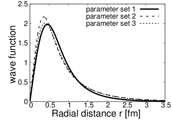
For the parameter set 2, we have found one bound state only for with the binding energy 27.2 MeV. This is significantly weaker than the result of set 1 and leads to the total mass closer to the experimentally observed one of . As mentioned above, the difference is due to the change in the pion decay constant. It seems that the use of the experimental value of is important to reproduce numerically the properties of the kaon and nucleon systems. For the parameter set 3, the binding energy is 32.9 MeV which is slightly larger, but in the similar order of magnitude to the result of set 2.
To understand better the bound state properties, in Table 1, we show root mean square radii for the baryon number distribution of the nucleon and for the kaon radial function. They are defined by
| (24) | |||||
| (25) |
where is the baryon charge density and is given by [27]
| (26) |
The baryon number radii are about 0.5 fm corresponding to the nucleon core size, while the kaon wave function extends up to 1 fm, indicating that the kaon is moving around the nucleon with weak binding. To see a bit more detail of Table 1, we observe that as the binding energy increases, in the order of set 2, set 3, and set 1, the hedgehog (baryon number) distribution increases, while the kaon distribution decreases. The fact that the bound state extends less for a larger binding energy is consistent with the general property of bound states.
In Figure 1, we have shown the normalized kaon wave functions for the three parameter sets. It is interesting to see that the wave function vanishes at the origin, although it is the s-wave. This is due to the presence of the repulsive core in the potential as we will see in the next subsection. In the large region, wave functions extends further for smaller binding energies, which explains the behavior of depending on the binding energy. The peak position of the wave function, however, is correlated with the attractive minima of the potential (as shown in the next subsection). Finally, we would like to emphasize that bound states exist with a binding energy of order ten MeV which is the typical order of hadronic interaction. This contrasts the Callan-Klebanov’s result [18, 19, 29], as we will discuss in the subsection III.3 in detail.
| [MeV] | B.E. [MeV] | [fm] | [fm] | ||
|---|---|---|---|---|---|
| parameter set 1 | 129 | 5.45 | 82.9 | 0.59 | 0.99 |
| parameter set 2 | 186 | 5.45 | 27.2 | 0.41 | 1.19 |
| parameter set 3 | 186 | 4.82 | 32.9 | 0.46 | 1.18 |
III.2 Potential
In this subsection, we study the potential for the kaon nucleon system. It has been already defined in the Klein-Gordon like equation (14) by in Eq. (17). Thus the potential carries the dimension of MeV2. Now it is convenient to define an alternative one in units of MeV which is used in a schrödinger-like equation. To do that, we first rewrite Eq. (14) in the following form
| (27) |
where
| (28) |
and
In Eq. (), , , and are given by Eq. (15), Eq. (16), and Eq. (17), respectively. This potential has the following properties. First, it is nonlocal and depends on the kaon energy. Second, it contains four components of the isospin independent and dependent, central and LS terms as we mentioned in subsection II.2. Third, near the origin, this potential behaves as a repulsive or an attractive force proportional to depending on the total isospin and total spin. Details of this behavior are discussed in Appendix.
Because the potential formally contains derivative, we make the following equivalent quantity
| (30) |
In this paper, we computed it by using the bound state wave function. Therefore, strictly speaking the potential derived here is for bound state. In principle it is also possible to calculate for other ’s by using scattering wave functions. The study of the scattering states will be discussed elsewhere.
The resulting is plotted in Figure 2 for the three parameter sets as used in the previous subsection. In the ordering of 1, 3, and 2, the potential minimum moves from outside to inside, and with the potential depth increasing. In accordance with this change, the shapes of the kaon wave functions have been explained in the previous subsection.

Now, it is instructive to investigate further properties in comparison with what we expect in the chiral theory. In the chiral theory, interaction is derived from the Weinberg-Tomozawa interaction (WT interaction) and is given by the following lagrangian [13, 14]
| (31) |
where and are the nucleon and the kaon isospin operators, respectively.
A feature of Eq. (31) is that the interaction strength is proportional to . Therefore, the interaction becomes stronger for smaller and vice versa. To see this relation in the present approach, we have computed the volume integral of the potential
| (32) |
and take the ratios of ’s with different ’s. In our parameter sets 1 and 2 with and 186 MeV, we find the ratio
| (33) |
which is compatible with . A small difference is considered due to the violation of SU(3) in the present ansatz of the bound state approach.
III.3 Comparisons with the Callan-Klebanov approach
In this subsection, we compare our results with those of Callan-Klevanov (CK). In thier approach for the hedgehog kaon system, the lowest bound state appears in the p-wave rather than s-wave with a strong binding energy of order hundred MeV [18, 19, 29]. We show the some results for parameter set 3 in Table 2, where is the kaon orbital angular momentum and is the effective angular momentum defined by [18, 19]
| (34) |
The p-wave bound state corresponds to and the s-wave to in the CK approach [18, 19]. From Table 2, we find that the kaon radii, , are about 0.5 fm for the p-wave and 0.9 fm for the s-wave in the CK approach 11 1 We have performed numerical calculations in the CK approach., which are substantially smaller than those of our present approach. These results for small radii seem consistent with their interpretation of the kaon hedgehog system as the strange quark and diquark system for hyperons.
| Callan-Klebanov approach | Our approach | Physical state | |||||
|---|---|---|---|---|---|---|---|
| B. E. [MeV] | [fm] | B. E. [MeV] | [fm] | ||||
| 0 | 1 | 61.7 | 0.93 | 0 | 32.9 | 1.18 | |
| 1 | 0 | 326.6 | 0.54 | — | — | — | |
In Figure 3, we show the potentials for the s- and p-wave bound states in the CK approach, which are defined similarly to the one of Eq. (30). For p-wave, the potential has a strong attraction at the origin. This causes the strong bound state as the ground state in the p-wave. For s-wave, we see a repulsive component toward the origin. This is caused by the centrifugal-like component due to the effective angular momentum . A similar structure is seen in our potential in Figure 2. We consider that the presence of the centrifugal-like potential in the CK approach is related to the presence of the repulsive core in our approach.

IV Summary
In this paper, we have constructed a new method for the study of kaon-nucleon systems and their interactions in the Skyrme model based on the bound state approach which Callan and Klebanov proposed [18, 19]. In our approach, we first quantize the hedgehog ansatz to generate the physical nucleon and introduce kaon fluctuations around it. This is the different point from the Callan-Klebanov approach, where they first introduce the kaon fluctuations around the hedgehog, and then the kaon-hedgehog system is quantized for hyperons. Although our method does not obey expansion systematically, we consider it suitable for a kaon bound system of small binding energy of order ten MeV or less.
As a general structure of interaction between isoscalar-pseudoscalar kaon and isospinor-spinor nucleon, the obtained potential contains central and spin-orbit terms with and without isospin dependence. A nontrivial finding is that there is either repulsion or attraction proportional to for small , depending on the kaon partial wave. For , the resulting potential turns out to contain the short range repulsion and the middle range attraction. Consequently, the kaon bound states obtain a weak binding energy. The presence of the repulsion should have an influence for the properties of high density kaonic nuclear matter. When term gives an attraction , the system becomes unstable. The present method, however, should not be applied to such a situation, where we need more microscopic approach.
In the present paper, we have focused our discussion on possible bound states. An extension to continuum states for kaon nucleon scattering is rather straightforward. As for kaon scatterings, Karliner and Mattis made a detailed investigation especially for higher partial waves [30, 31]. We plan to study scattering states from lower to higher partial waves. So far we have considered only kaon-nucleon channel, but it is well known that channel is also important especially for the discussion of . It is another interesting extension of the present study, which we hope to report elsewhere.
Acknowledgements.
We thank Noriyoshi Ishii and Takuya Sugiura for useful discussions. This work is supported in part by the Grant-in-Aid for Science Research (C) 26400273.Appendix A
In this appendix, we show an outline to derive the potential Eq. (17). Substituting our ansatz Eq. (11) for the lagrangian Eq. (1), and expanding it up to second order of the kaon fields, we obtain the following lagrangian
| (35) |
where
| (36) |
and
| (37) | |||||
In these equations, we have defined
| (38) |
| (39) |
| (40) | |||||
| (41) |
where the hedgehog ansatz and are given by Eq. (10), and is the baryon current which is given by [27]
| (42) |
From Eq. (37), we derive the equation of motion for the kaon Eq. (14) and the potential Eq. (17) with each term given by
| (43) | |||||
| (45) |
and
| (46) |
where
| (47) |
and
| (48) |
The moment of inertia is given by
| (49) |
The last terms of Eq. (43) and Eq. (45) are derived from the Wess-Zumino term, which is attractive for the potential and repulsive for the potential. These equations are general for any partial waves of the kaon. For instance, the -wave potential is obtained by setting and removing the terms including in Eq. (17).
Now we discuss two features of the potential, the relation with the Weinberg-Tomozawa interaction (WT interaction) [13, 14] and the short range behaviors. To see the essential aspect of the WT interaction for the kaon-nucleon interaction, let us look at the leading contribution from the pion fields, derived from the kinetic term where the covariant derivative in the lagrangian Eq. (37) is given by
| (50) |
with
| (51) |
and given by Eq. (7). Picking up the terms of order , we find
| (52) | |||||
where we have defined . We note that the first line of Eq. (52) takes the form of the product of the isospin vector currents of the kaon and the pion fields.
For the kaon and nucleon interaction, we first substitute the hedgehog ansatz for the pion field,
| (53) |
Then, we rotate the hedgehog ansatz in SU(2) space
| (54) |
Substituting Eq. (53) and Eq. (54) for Eq. (52), the leading contribution of the WT interaction is
| (55) |
where is given by Eq. (49).
On the other hand, in our approach, we obtain the following contributions from the kinetic term in the lagrangian Eq. (37) using our ansatz
| (56) | |||||
Comparing Eq. (55) with Eq. (56), we find that they coinside each other up to the leading order of .
Next, we consider how the potential behaves near the origin. From the equation of motion for [27], the behavior of near the origin is given by
| (57) |
| attractive | repulsive | |
| repulsive ( and ) | ||
| repulsive | repulsive |
References
- [1] R. H. Dalitz and S. F. Tuan, Phys. Rev. Lett. 2, 425 (1959). doi:10.1103/PhysRevLett.2.425
- [2] R. H. Dalitz and S. F. Tuan, Annals Phys. 10, 307 (1960). doi:10.1016/0003-4916(60)90001-4
- [3] A. N. Ivanov, P. Kienle, J. Marton and E. Widmann, nucl-th/0512037.
- [4] N. V. Shevchenko, A. Gal, J. Mares and J. Revai, Phys. Rev. C 76, 044004 (2007) doi:10.1103/PhysRevC.76.044004 [arXiv:0706.4393 [nucl-th]].
- [5] Y. Ikeda and T. Sato, Phys. Rev. C 76, 035203 (2007) doi:10.1103/PhysRevC.76.035203 [arXiv:0704.1978 [nucl-th]].
- [6] A. Dote, T. Hyodo and W. Weise, Nucl. Phys. A 804, 197 (2008) doi:10.1016/j.nuclphysa.2008.02.001 [arXiv:0802.0238 [nucl-th]].
- [7] T. Nishikawa and Y. Kondo, Phys. Rev. C 77, 055202 (2008) doi:10.1103/PhysRevC.77.055202 [arXiv:0710.0948 [hep-ph]].
- [8] T. Yamazaki and Y. Akaishi, Phys. Lett. B 535, 70 (2002). doi:10.1016/S0370-2693(02)01738-0
- [9] Y. Akaishi and T. Yamazaki, Phys. Rev. C 65, 044005 (2002). doi:10.1103/PhysRevC.65.044005
- [10] B. Borasoy, R. Nissler and W. Weise, Eur. Phys. J. A 25, 79 (2005) doi:10.1140/epja/i2005-10079-1 [hep-ph/0505239].
- [11] T. Hyodo and W. Weise, Phys. Rev. C 77, 035204 (2008) doi:10.1103/PhysRevC.77.035204 [arXiv:0712.1613 [nucl-th]].
- [12] Y. Ikeda, T. Hyodo and W. Weise, Nucl. Phys. A 881, 98 (2012) doi:10.1016/j.nuclphysa.2012.01.029 [arXiv:1201.6549 [nucl-th]].
- [13] S. Weinberg, Phys. Rev. Lett. 17, 616 (1966). doi:10.1103/PhysRevLett.17.616
- [14] Y. Tomozawa, Nuovo Cim. A 46, 707 (1966). doi:10.1007/BF02857517
- [15] T. H. R. Skyrme, Proc. Roy. Soc. Lond. A 260, 127 (1961). doi:10.1098/rspa.1961.0018
- [16] J. K. Perring and T. H. R. Skyrme, Nucl. Phys. 31, 550 (1962). doi:10.1016/0029-5582(62)90774-5
- [17] T. H. R. Skyrme, Nucl. Phys. 31, 556 (1962). doi:10.1016/0029-5582(62)90775-7
- [18] C. G. Callan, Jr. and I. R. Klebanov, Nucl. Phys. B 262, 365 (1985). doi:10.1016/0550-3213(85)90292-5
- [19] C. G. Callan, Jr., K. Hornbostel and I. R. Klebanov, Phys. Lett. B 202, 269 (1988). doi:10.1016/0370-2693(88)90022-6
- [20] J. Wess and B. Zumino, Phys. Lett. B 37, 95 (1971). doi:10.1016/0370-2693(71)90582-X
- [21] E. Witten, Nucl. Phys. B 223, 422 (1983). doi:10.1016/0550-3213(83)90063-9
- [22] E. Witten, Nucl. Phys. B 223, 433 (1983). doi:10.1016/0550-3213(83)90064-0
- [23] P. Ring and P. Schuck, The Nuclear Many-Body Problem (Springer, New York, 1980).
- [24] M. Praszalowicz, Phys. Lett. B 158, 264 (1985). doi:10.1016/0370-2693(85)90968-2
- [25] H. Yabu and K. Ando, Nucl. Phys. B 301, 601 (1988). doi:10.1016/0550-3213(88)90279-9
- [26] I. Zahed and G. E. Brown, Phys. Rept. 142, 1 (1986). doi:10.1016/0370-1573(86)90142-0
- [27] G. S. Adkins, C. R. Nappi and E. Witten, Nucl. Phys. B 228, 552 (1983). doi:10.1016/0550-3213(83)90559-X
- [28] K. A. Olive et al. [Particle Data Group Collaboration], Chin. Phys. C 38, 090001 (2014). doi:10.1088/1674-1137/38/9/090001
- [29] N. Itzhaki, I. R. Klebanov, P. Ouyang and L. Rastelli, Nucl. Phys. B 684, 264 (2004) doi:10.1016/j.nuclphysb.2004.02.004 [hep-ph/0309305].
- [30] M. Karliner and M. P. Mattis, Phys. Rev. D 34, 1991 (1986). doi:10.1103/PhysRevD.34.1991
- [31] M. Karliner, Phys. Rev. Lett. 57, 523 (1986). doi:10.1103/PhysRevLett.57.523