Optimal DoF Region for the Asymmetric Two-Pair MIMO Two-Way Relay ChannelThanks: Part of this work is submitted to the 2016 IEEE Global Telecommunications Conference. Kangqi Liu and Meixia Tao are with the Department of Electronic Engineering, Shanghai Jiao Tong University, Shanghai, China (Emails: k.liu.cn@ieee.org, mxtao@sjtu.edu.cn). Xiaojun Yuan is with the School of Information Science and Technology, ShanghaiTech University, Shanghai, China (Emails: yuanxj@shanghaitech.edu.cn).
Abstract
In this paper, we study the optimal degrees of freedom (DoF) region for the two-pair MIMO two-way relay channel (TWRC) with asymmetric antenna setting, where two pairs of users exchange information with the help of a common relay. Each user is equipped with antennas, for , and the relay is equipped with antennas. First, we derive an outer bound of the DoF region by using the cut-set theorem and the genie-message approach. Then, we propose a new transmission scheme to achieve the outer bound of the DoF region. Due to the asymmetric data exchange, where the two users in each pair can communicate a different number of data streams, we not only need to form the network-coded symbols but also need to process the additional asymmetric data streams at the relay. This is realized through the joint design of relay compression matrix and source precoding matrices. After obtaining the optimal DoF region, we study the optimal sum DoF by solving a linear programming problem. From the optimal DoF region of this channel, we show that in the asymmetric antenna setting, some antennas at certain source nodes are redundant and cannot contribute to enlarge the DoF region. We also show that there is no loss of optimality in terms of the sum DoF by enforcing symmetric data exchange, where the two users in each pair are restricted to communicate the same number of data streams.
Index Terms:
Multiple-input multiple-output, two-way relay channel, interference alignment, physical-layer network coding, signal alignment, degrees of freedom.I Introduction
Due to the great promises in power reduction, coverage extension, and throughput enhancement, wireless relaying has been an important ingredient in both ad hoc and infrastructure-based wireless networks [1, 2, 3]. Nowadays, a relay has become very much like a wireless gateway where multiple users share a common relay and communicate with each other. A typical representative is the two-way relay channel (TWRC) [4, 5, 6], where two users exchange information with each other through a relay. The success of two-way relaying owes to the invention of physical layer network coding (PLNC) [7, 8], which almost doubles the spectral efficiency compared with traditional one-way relaying [9, 10].
A natural generalization of TWRC in multi-user and multi-antenna scenarios is known as multi-user MIMO (MU-MIMO) TWRC [11], where there are source nodes and one relay node, all equipped with multiple antennas, and each source node can exchange independent messages with an arbitrary set of other nodes via the relay node. It includes several special cases: -user MIMO Y channel [12], multi-pair MIMO two-way relay channel [13, 14, 15, 16, 17], and -cluster -user MIMO multiway relay channel [18, 19]. However, the exact capacity analysis for these channels is extremely challenging, only constant-gap capacity is known in the simplest scenario [20, 21]. As a measure of the approximate capacity in the high signal-to-noise ratio (SNR) region, degrees of freedom (DoF) [22] specifies how the transmission rate scales as the transmission power goes to infinity. DoF also characterizes the number of interference-free data streams that can be communicated in a given channel.
The DoF analysis for various MU-MIMO TWRC has attracted much attention in the literature [23, 24, 25, 26, 27, 28, 11, 18, 29, 19, 30, 31]. Such analysis is tractable mainly due to signal alignment proposed in [23] as an integration of PLNC and interference alignment (IA) [32, 33]. Recent developments include signal alignment for MIMO Y channel [23], signal group alignment for -user MIMO Y channel [25], signal pattern approach for -cluster -user MIMO multiway relay channel [28], and generalized signal alignment (GSA) for the arbitrary MU-MIMO TWRC [11]. The main results are summarized in Table I. Here, denotes the number of antennas at the relay node, denotes the number of antennas at each user for the asymmetric antenna setting, and denotes the number of antennas at each user for the symmetric antenna setting. It is seen from Table I that the complete characterization of the sum DoF is only available for users with symmetric antenna setting. The analysis of the sum DoF and the DoF region in the general case with asymmetric antenna setting largely remains open.
| Channel Model | Antenna setting | Sum DoF/DoF region | Antenna configuration for optimal sum DoF/DoF region | Status | Reference |
| MIMO Y channel | Symmetric | Sum DoF | Done | [23, 24] | |
| Asymmetric | Sum DoF | Done | [24] | ||
| Four-user MIMO Y channel | Symmetric | Sum DoF | Done | [27, 11] | |
| -user MIMO Y channel | Symmetric | Sum DoF | Partial | [11] | |
| DoF region | Partial | [31] | |||
| Asymmetric | Sum DoF | Partial | [29] | ||
| Two-pair MIMO TWRC | Symmetric | Sum DoF | Done | [11] | |
| -pair MIMO TWRC | Symmetric | Sum DoF | Partial | [11] | |
| -cluster -user MIMO multi-way relay channel | Asymmetric | Sum DoF | Refer to Theorem 2-4 in [18] | Partial | [18] |
| Two-pair MIMO TWRC | Asymmetric | Sum DoF | Done | This paper | |
| DoF region |
In this work, we aim to make some progress toward the DoF analysis of the MU-MIMO TWRC with asymmetric antenna setting. To this end, we have succeeded in providing the complete characterization of both DoF region and sum DoF for asymmetric two-pair MIMO TWRC with antenna configuration for the first time. The main contributions and results of this paper are as follows.
We first derive an outer bound of the DoF region for any antenna configuration by using the cut-set theorem and the genie-message approach. Then we propose a new transmission scheme based on the idea of GSA [11] to achieve the outer bound of the DoF region. Let denote the number of interference-free data streams to be transmitted from (to) user to (from) its pairing user . The key idea of the proposed achievable scheme is to align pairs of bidirectional signals to be exchanged between user and its pairing user in a same compressed subspace so as to form network-coded symbols, and project the additional unidirectional data streams from one user to another on a different subspace for complete decoding. This is realized through the joint design of relay compression matrix and source precoding matrices. In [24], the optimal sum DoF of the MIMO Y channel with asymmetric antenna setting is characterized by using signal alignment and antenna deactivation techniques. It is pointed out that symmetric data exchange, where the two users in each pair communicate the same number of data streams, can achieve the optimal sum DoF. In [29], the sum DoF of an arbitrary MU-MIMO TWRC is analyzed under an asymmetric antenna setting. But the analysis is limited to symmetric data exchange. In contrast with the scheme in [24] and [29], we need not only to construct network-coded symbols but also to process the additional asymmetric data streams at the relay, which enables us to obtain the DoF region rather than just the sum DoF. In [31], the optimal DoF region of the -user MIMO Y channel with symmetric antenna setting is studied by using channel diagonalization and cyclic communication techniques. Their transmission scheme is only applicable when the antenna configuration satisfies . By comparing with the scheme in [31], our transmission scheme is applicable for all different antenna configurations.
After obtaining the optimal DoF region, determining the optimal sum DoF becomes a linear programming problem. By analyzing this problem, we find that enforcing symmetric data exchange within each user pair does not lose any optimality in terms of the sum DoF. Based on this finding, the linear programming problem is greatly simplified and we are able to obtain the optimal sum DoF explicitly at all antenna configurations.
The rest of the paper is organized as follows. In Section II, we present the system model. In Section III, we introduce the main results and show the insights of the results. The proof of DoF-region converse and DoF-region achievability are presented in Section IV and Section V, respectively. In Section VI, we show the optimal sum DoF of the channel. Finally, we conclude the paper in Section VII.
Notations: Scalars, vectors, and matrices are denoted by lowercase regular letters, lowercase bold letters, and uppercase bold letters, respectively. and denote the transpose and the Hermitian transpose, respectively. rank stands for the rank of . I is the identity matrix. and stand for the column space and the null space of the matrix , respectively. denotes the binomial coefficient indexed by and .
II Channel Model

Consider a discrete memoryless asymmetric two-pair MIMO TWRC as shown in Fig. 1, where users and form a pair to exchange information and users and form another pair to exchange information, both with the help of a common relay. Each user is equipped with antennas, and the relay is equipped with antennas. Without loss of generality, we assume that
| (1) |
Denote by the channel matrix from user to the relay for channel use , and by the channel matrix from the relay to user . It is assumed that the entries of the channel matrices are drawn independently from a continuous distribution, which guarantees that the channel matrices have full rank with probability one. Perfect channel knowledge is assumed to be available at each node, and all the nodes in the network are assumed to be full duplex. The message transmitted from user to its pairing user is denoted by , and is independent of each other. Each is encoded using a codebook with size , where is the codeword length and is the information rate of . Note that can be different from due to the asymmetric antenna setting, different channel gain, or different rate requirement on user and .
The message exchange takes place in two phases: the multiple access (MAC) phase and the broadcast (BC) phase. In the MAC phase, all the users transmit their signals to the relay. The received signal for the channel use at the relay, denoted by , is given by
| (2) |
where denotes transmitted signal from user with average power constraint , and denotes the additive white Gaussian noise (AWGN) vector for the channel use with each element being independent, and having zero mean and unit variance.
Upon receiving in (2), the relay processes these messages to obtain a mixed signal with average power constraint , and broadcasts to all the users. The received signal for the channel use at user , denoted by , is given by
| (3) |
where denotes the AWGN vector for the channel use with each element being independent, and having zero mean and unit variance.
Each user will decode its desired message, denoted by , based on the received signals and its own transmitted message. Let denote the achievable information rate of the message under the power constraint . Here, we say that a rate tuple is achievable if
| (4) |
The DoF of message is defined as
| (5) |
The sum DoF is defined as
| (6) |
The DoF region is defined as [32]
| (7) |
where is the capacity region of the asymmetric two-pair MIMO TWRC, which is the set of all achievable rate tuples . The goal of this work is to characterize the optimal DoF region, denoted by , as well as the optimal sum DoF, denoted by , for the considered asymmetric two-pair MIMO TWRC with antenna configuration .
III Main Results
The main findings of this paper are summarized in the following theorem and corollary.
Theorem 1: For the asymmetric two-pair MIMO TWRC with antenna configuration , the optimal DoF region can be expressed as
| (8a) | ||||
| (8b) | ||||
| (8c) | ||||
| (8d) | ||||
| (8e) | ||||
| (8f) | ||||
| (8g) | ||||
| (8h) | ||||
| (8i) | ||||
| (8j) | ||||
| (8k) | ||||
| (8l) | ||||
Corollary 1: For the asymmetric two-pair MIMO TWRC with antenna configuration , the optimal sum DoF is given as follows:
- 1.
When ,
(9) - 2.
When ,
(10) - 3.
When ,
(11)
The DoF converse of Theorem 1 is proved in Section IV via the cut-set theorem and the genie-message approach. The achievability of Theorem 1 is proved in Section V. The proof of Corollary 1 is presented in Section VI.
Remark 1 (Redundant antennas): It is observed from Theorem 1 that the DoF only depends on and does not depend on when . This means that if the relay antenna number is large enough, the smaller antenna number within each user pair limits the DoF. Hence, there are redundant antennas at user , and redundant antennas at user . Likewise, when , the DoF only depends on and does not depend on . Hence, there are redundant antennas at user .
Remark 2: (Connection to symmetric two-pair MIMO TWRC): When , for , the sum DoF characterized in Corollary 1 reduces to , which is consistent with the results in [11].
Remark 3: (Comparison to the existing work [18]): The authors in [18] study the sum DoF for the asymmetric -cluster -user MIMO multi-way relay channel. In the special case when , the channel in [18] reduces to our considered two-pair MIMO TWRC. However, the maximum sum DoF results in [18] are neither optimal nor complete, while our sum DoF results in Corollary 1 are optimal and complete.
IV DoF-region converse
The first four bounds in (8) can be proved easily from the cut-set theorem [34]. That is, since each user has antennas only, the DoF of the transmitted or received message for user cannot be greater than .
We now prove the bound (8e) by using the genie-aided message approach as in [24, 27, 26, 11]. By the converse assumption, each user can decode its intended message with its own transmitted messages as side information. Given the fact that the signal received by each user is a degraded version of the signal received at the relay, if a genie provides the side information to the relay, then the relay is able to decode . As such, we provide as the genie message to the relay and obtain the following bound:
| (12a) | ||||
| (12b) | ||||
| (12c) | ||||
| (12d) | ||||
| (12e) | ||||
| (12f) | ||||
where (12a) follows from the Fano’s inequality; (12b) follows from the data processing inequality; (12c) follows from the fact that when is independent of ; (12d) follows from the chain rule. Dividing through both sides of (12) and letting and , we obtain the bound (8e). Similarly, (8f)-(8h) can be obtained.
Next, we prove the bound (8i) through the genie-message approach. Note that there are in total four messages received at the relay. If the message and are known at the relay, then the relay can decode provided . Hence, we provide as a genie message to the relay in the case of in the first step. By the converse assumption, we can obtain the following bound:
| (13a) | ||||
| (13b) | ||||
| (13c) | ||||
| (13d) | ||||
| (13e) | ||||
Dividing through both sides of (13) and letting and , we obtain
| (14) |
when .

What remains is to consider the case of . Again, if the messages, and , are already known at the relay, the unknown messages at the relay remain , which is illustrated in Fig. 2. It can be seen that there is an intersection subspace of and with dimension . We separate the message into two parts as and , where is located in the intersection subspace and is orthogonal to the intersection subspace. Then, if is provided as a genie message to the relay, the relay can decode and surely. Hence, we provide as a genie message to the relay. By the converse assumption, we obtain the following bound:
| (15a) | ||||
| (15b) | ||||
| (15c) | ||||
| (15d) | ||||
| (15e) | ||||
| (15f) | ||||
Dividing through both sides of (15) and letting and , we obtain
| (16) |
when . Combining (14) and (16), we obtain the bound (8i). Similarly, (8j)-(8l) hold, which concludes the proof.
V DoF-region achievability
In this section, we prove the achievability of the optimal DoF region for the asymmetric two-pair MIMO TWRC. We first illustrate the main idea of our proposed transmission scheme using an example. Then we consider the general case and present the achievable schemes in three different antenna configurations: (I) ; (II) ; (III) .
V-A An example with
In this subsection, we illustrate how to achieve the DoF tuple under the antenna configuration . In this example, there are pairs of data streams to be exchanged between user and , and pair of data streams to be exchanged between user and user . In addition to that, user has more data streams to communicate with user and user has more data streams for user .
During the MAC phase, the signal received at the relay can be rewritten as
| (17) |
Here, and are the pair of signals to be exchanged between user and user , and are the pair of signals to be exchanged between user and user , and represent the additional signals sent from user and user to user and user , respectively; , , , , , and are the corresponding precoding matrices. According to the GSA principle proposed in [11]11 1 GSA refers to that a pair of signals to be exchanged are aligned at a same compressed subspace at the relay through the joint design of relay compression matrix and source precoding matrices., we need to jointly design a full-rank relay compression matrix and all the precoding matrices and such that:
| (18a) | ||||
| (18b) | ||||
| (18c) | ||||
| (18d) | ||||
A signal space illustration is given in Fig. 3. Specifically, condition (18a) means that the relay needs to align the signal pair in a subspace to form network-coded symbols, and condition (18b) means to align the signal pair in another subspace to form network-coded symbols. Condition (18c) is to ensure the separability of and at user , and likewise condition (18d) is to ensure the separability of and at user . In total, the relay needs to decode independent symbols and we should choose according to [11].
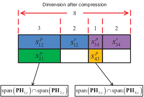
However, in [11], the authors only provide the necessary and sufficient condition for the GSA equation to hold under the symmetric antenna setting when . In the following lemma, we give the necessary and sufficient condition for (18a) and (18b) to hold under the general asymmetric antenna setting.
Lemma 1: The GSA equations (18a) and (18b) hold if and only if there are at least basis vectors of that lie in the null space of for all user pair with .
Proof:
The proof is similar to the proof of Theorem 4 in [11] and thus omitted here. ∎
It is noted that the dimension of the intersection space between and is 3, which is enough to align the data streams and . The difficulty is how to align and as there is no intersection subspace between and . To this end, we first design , and for (18b) to hold. According to Lemma 1, there should be one row of that lies in the left null space for (18b) to hold. Thus, we design such that
where is a submatrix satisfying
| (21) |
or equivalently,
| (22) |
and is a submatrix that can be designed randomly as long as has full row rank. For instance, we can choose . Then, can be expressed as
with rank . We then design and as
Here, and exist because the dimension of the null space of is .
Next, we design and for (18a) to hold. It is noted that the rank of is 8 and hence the null space of the matrix has dimension of 3. We can design and as
Once are designed, (or ) can be designed randomly as long as and have full column rank in order to meet (18c) and (18d). The signal after compression at the relay can be expressed as
| (29) |
Thus far, the relay is able to decode the network-coded symbols, and , as well as the remaining symbols, and , by using an zero-forcing matrix
| (30) |
The decoded symbol vector, , can be expressed as
| (35) |
We next introduce the transmission scheme in the BC phase for each user to decode its desired message. The signal received at user with receiving matrix can be expressed as
| (36) |
where denotes a compression matrix in the BC phase and denotes a zero-forcing matrix in the BC phase.
Due to the symmetry between the MAC and BC phases, we redefine as
| (37) | ||||
satisfying
| (40a) | ||||
| (40b) | ||||
Note that there exists symmetry between the design of and , and , as well as and . Then the zero-forcing matrix in the BC phase can be designed as
The signal received at user in (36) can be rewritten as
| (45) | ||||
Finally, each user can decode its desired signal after applying self-interference cancellation. The DoF tuple under the antenna configuration is thus achievable.
From this example, we see that the main challenge lies in the design of the relay compression matrix at the MAC phase in response to the asymmetric information exchange within each user pair. To tackle this challenge, we have extended the GSA principle in [11] to the asymmetric antenna setting as in Lemma 1. In the next subsection, we extend the idea to the general antenna configuration and present the achievable scheme to obtain the optimal DoF region when the number of antennas at the relay falls into three different regions.
V-B
In this subsection, we present the DoF-region achievability when . In this case, the DoF region (8) in Theorem 1 can be simplified as
| (48a) | ||||
| (48b) | ||||
| (48c) | ||||
| (48d) | ||||
| (48e) | ||||
| (48f) | ||||
| (48g) | ||||
| (48h) | ||||
Due to the symmetry between user and its pairing user as well as the symmetry between user and its pairing user , we focus on the DoF tuple where and . Thus, besides (or ) pairs of independent data streams to be exchanged and aligned between user (or ) and user (or ), there are additional (or ) data streams to be sent from user (or ) to user (or ). We assume that user and user only utilize and antennas, respectively, in this case by antenna deactivation.
During the MAC phase, since the relay needs to decode independent data streams (including both network-coded symbols and individual symbols), we compress the signal received at the relay by a full-rank compression matrix , where
| (49) |
It is worth mentioning that is satisfied for all DoF tuples in from (8e)-(8h). In the -dimensional compressed subspace of the relay, the first dimensions are used for the pairs of data streams transmitted from user and user to align so as to form network-coded symbols. Similarly, the second dimensions are used for the pairs of data streams from user and user . The remaining and dimensions are used to decode the additional data streams sent from user to user and the additional data streams sent from user to user , respectively.
According to Lemma 1, we design , , , and such that
| (50a) | ||||
| (50b) | ||||
| (50c) | ||||
| (50d) | ||||
Here, the definitions of the precoding matrices and are given in (17). We separate the design of and into four cases: (I) and ; (II) and ; (III) and ; (IV) and ;
V-B1 Case I
First, we consider the DoF tuples satisfying and . We separate into three parts as
where is a submatrix, is a , and is a submatrix. Here, exists due to the fact of and (48a)-(48d). We design and as
| (54) | ||||
| (55) |
can be designed randomly as long as has full row rank. Here, exists because the dimension of the null space of is , which is greater than or equal to from the fact (48e); exists because the dimension of the null space of is , which is greater than or equal to from the fact (48g).
Then, can be expressed as
with rank . We then design the precoding matrices and as
Here, and exists because the dimension of the null space of is . Therefore, the alignment condition in (50a) is satisfied.
Similarly, can be expressed as
with rank . We then design the precoding matrices and as
Here, and exists because the dimension of the null space of is . Thus, the alignment condition (50b) is satisfied. The remaining two precoding matrices and can be designed randomly as long as and have full column rank, so that (50c) and (50d) hold. For presentation simplicity, the design of will be skipped in the remaining part of this section since the criterion is the same.
V-B2 Case II
Second, we consider the DoF tuples satisfying and . We separate into two parts as
where is a submatrix, is a . We design by following (54), and design randomly as long as has full row rank. Then, can be expressed as
with rank . We design and according to (V-B1). Here, and exists because the dimension of the null space of is . The rank of is . We design and according to (V-B1). Here, and exists because the dimension of the null space of is , which is greater than or equal to from the fact that .
V-B3 Case III
Third, we consider the DoF tuples satisfying and . This case can be converted into Case II by swapping the user indexes: and . Then, the proof follows immediately from that of Case II.
V-B4 Case IV
Finally, we consider the DoF tuples satisfying and . This case is trivial since we can design randomly as long as it has full row rank. The rank of is . We design and according to (V-B1). Here, and exists because the dimension of the null space of is , which is greater than or equal to due to . The rank of is . We design and according to (V-B1). Here, and exists because the dimension of the null space of is , which is greater than or equal to due to .
Combining Case I-IV, we have shown the design of , and to meet (50). The signal after compression at the relay can be expressed similarly as in (29). Then we detect the network-coded symbols, and , as well as the remaining symbols, and , by introducing a zero-forcing matrix as in (30).
The above precoding design directly carries over to the BC phase due to the symmetry between the MAC and the BC phases and is thus omitted. Therefore, all the DoF tuples in are achievable.
V-C
In this section, we present the DoF-region achievability when and . In this case, the DoF region (8) in Theorem 1 can be simplified as
| (70a) | ||||
| (70b) | ||||
| (70c) | ||||
| (70d) | ||||
| (70e) | ||||
| (70f) | ||||
| (70g) | ||||
| (70h) | ||||
Due to the symmetry between the two users in a pair, it suffices to only consider a DoF tuple with and . We assume that user only utilizes antennas in this case by antenna deactivation.
The basic idea is the same as that in the previous subsection. We only present the design of and to satisfy (50) here. We separate the design of and into two cases: (I) ; (II) .
V-C1 Case I
First, we consider the DoF tuples satisfying . The example we illustrated in Section V-A belongs to this case. We separate into two parts as
where is a submatrix, and is a . We design as
| (73) |
and is designed randomly as long as has full row rank. Here, exists because the dimension of the null space of is , which is greater than or equal to from (70g). Then, the rank of is . We design and according to (V-B1). Here, and exists because the dimension of the null space of is , which is greater than or equal to from (70e). Then, can be expressed as
with rank . We design and according to (V-B1). Here, and exists because the dimension of the null space of is .
V-C2 Case II
Second, we consider the DoF tuples satisfying . We design randomly, which is a full-rank matrix. The rank of is . We design and according to (V-B1). Here, and exists because the dimension of the null space of is , which is greater than or equal to from (70e). The rank of is . We design and according to (V-B1). Here, and exists because the dimension of the null space of is , which is greater than or equal to from .
The above precoding design directly carries over to the BC phase due to the symmetry between the MAC and the BC phases and is thus omitted. Therefore, all the DoF tuples in are achievable.
V-D Case 3:
In this section, we present the DoF-region achievability when . In this case, the DoF region (8) in Theorem 1 can be simplified as
| (76a) | ||||
| (76b) | ||||
| (76c) | ||||
| (76d) | ||||
| (76e) | ||||
| (76f) | ||||
| (76g) | ||||
| (76h) | ||||
| (76i) | ||||
| (76j) | ||||
| (76k) | ||||
| (76l) | ||||
Due to the symmetry between the two users in a pair, it suffices to focus on a DoF tuple satisfying and .
The basic idea is the same as that in the previous subsections. We only present the design of and to satisfy (50) here. Once we obtain and , then can be designed as (30), (40) and (V-A), similarly. We use the antenna deactivation method at the relay, i.e., the relay only utilize antennas. The rank of is . We design and according to (V-B1). Here, and exists because the dimension of the null space of is , which is greater than or equal to from (76i). The rank of is . We design and according to (V-B1). Here, and exists because the dimension of the null space of is , which is greater than or equal to from (76k).
The above precoding design directly carries over to the BC phase due to the symmetry between the MAC and the BC phases and is thus omitted. Therefore, all the DoF tuples in are achievable.
VI Sum DoF (Proof of Corollary 1)
In this section, we prove the optimal sum DoF of the asymmetric two-pair MIMO TWRC in Corollary 1.
Given the optimal DoF region in Theorem 1, the optimal sum DoF can be found by solving the following optimization problem:
| (77) |
It is clear that problem (77) is a linear optimization problem with 4 variables and 12 constraints. The optimal solution can be obtained numerically [35]. However, we are interested in finding its closed-form expression to complete the DoF analysis. The feasible region for the problem (77), i.e., the optimal DoF region specified by (8a)-(8l), is a polytope in a -dimensional space. The optimal solution to must be located in one of the vertexes of the polytope. But it is not straightforward to find the optimal solution, as there are candidate vertexes22 2 Each candidate vertex is given by letting 4 out of the 12 inequalities in (8) take equality.. This motivates us to reduce the search space by exploiting the structural properties of the optimal solution of problem (77). To proceed, we shall present the following useful lemma.
Lemma 2: If a DoF tuple is an optimal solution to (77), then is also an optimal solution to (77), where and .
Proof:
It is clear that the objective value for and are the same. Thus, it remains to show that is also located in the polytope generated by . We show this in three steps.
Step 2 (Constraints (8e)-(8h)): Since is a feasible solution to (77), from (8e)-(8h), we have
| (78) |
Then
| (79) |
Therefore, is a feasible DoF tuple and Lemma 2 is proved. ∎
Lemma 2 reveals that enforcing symmetric pairwise data exchange, i.e., , does not sacrifice the optimality of the sum DoF. Based on this, the optimization problem (77) can be simplified as
| (80a) | ||||
| (80b) | ||||
| (80c) | ||||
| (80d) | ||||
| (80e) | ||||
| (80f) | ||||
Here the problem (80) only contains two variables and six constraints. It is now more tractable to search over all the vertexes of the new polytope generated by (80a)-(80f). The optimal sum DoF and the corresponding vertexes are thus obtained and presented in Table II , Table III and Table IV .
| Optimal sum DoF | Achieving vertex | ||
|---|---|---|---|
|
| |||
|
| |||
|
| |||
|
|
| Optimal sum DoF | Achieving vertex | ||
|---|---|---|---|
|
| |||
|
| |||
|
| |||
|
| |||
|
|
| Optimal sum DoF | Achieving vertex | ||
|---|---|---|---|
|
| |||
| See Appendix A | |||
|
| |||
|
| |||
|
|
VII Conclusion
In this work, we have presented a complete characterization of the optimal DoF region of the asymmetric two-pair MIMO TWRC. The proposed transmission scheme takes into account the asymmetric data exchange within each user pair and designs the relay compression matrix and all the source precoding matrices jointly using the generalized signal alignment principle. We have also derived the optimal sum DoF of the asymmetric two-pair MIMO TWRC. Our results reveal that in the asymmetric antenna setting, some antennas at certain source nodes are redundant and do not contribute to enlarge the DoF region. Our results also reveal that enforcing symmetric data exchange within each user pair does not lose the optimality of the sum DoF.
For the multi-pair MIMO TWRC with more than 2 pairs, the optimal sum DoF is still unknown even for symmetric antenna setting. Thus, determining the optimal DoF region for the multi-pair MIMO TWRC still remains open.
Appendix A
Here, we present the vertex that achieves the optimal sum DoF in 8 cases. Define
| (81) |
- •
If and , then the achieving vertex is .
- •
If and , then antenna deactivation is applied at user and user in order to set , where and are respectively the numbers of antennas utilized at users and after antenna deactivation. The achieving vertex is .
- •
If and , then the achieving vertex is .
- •
If and , then antenna deactivation is applied at user , user , and user in order to set . The achieving vertex is .
- •
If and , then the achieving vertex is .
- •
If , then antenna deactivation is applied at user , user , and user to ensure . The achieving vertex is .
- •
If and , then the achieving vertex is .
- •
If and , then antenna deactivation is applied at user , user , user , and user to ensure . The achieving vertex is .
References
- [1] S. G. Y. R. Editors: Y. Hua, D. W. Bliss and Y. Sung, “Theories and methods for advanced wireless relays: Issue I,” IEEE J. Sel. Areas Commun., vol. 30, no. 8, Sept. 2012.
- [2] M. Gastpar and M. Vetterlj, “On the capacity of wireless networks: the relay case,” in Proc. IEEE INFOCOM., vol. 3, 2002, pp. 1577–1586.
- [3] G. Kramer, M. Gastpar, and P. Gupta, “Cooperative strategies and capacity theorems for relay networks,” IEEE Trans. Inf. Theory, vol. 51, no. 9, pp. 3037–3063, Sep. 2005.
- [4] B. Rankov and A. Wittneben, “Achievable rate regions for the two-way relay channel,” in Proc. IEEE Int. Symp. Inf. Theory, no. 1668-1672, 2006.
- [5] ——, “Spectral efficient protocols for half-duplex fading relay channels,” IEEE J. Sel. Areas Commun., vol. 25, no. 2, Feb. 2007.
- [6] R. Wang and M. Tao, “Joint source and relay precoding designs for MIMO two-way relaying based on MSE criterion,” IEEE Trans. Signal Process., vol. 60, no. 3, pp. 1352 – 1365, March 2012.
- [7] S. Zhang, S. Liew, and P. Lam, “Physical layer network coding,” in Proc. ACM MobiCom, Sep. 2006, pp. 63–68.
- [8] S. Katti, S. Gollakota, and D. Katabi, “Embracing wireless interference: analog network coding,” in Proc. ACM SIGCOMM., Sep. 2007, pp. 397–408.
- [9] R. Vaze and R. W. Heath, “Capacity scaling for MIMO two-way relaying,” in Proc. IEEE Int. Symp. Inf. Theory, Jun. 2007, pp. 1451 – 1455.
- [10] X. Yuan, T. Yang, and I. B. Collings, “Multiple-input multiple-output two-way relaying: A space-division approach,” IEEE Trans. Inf. Theory, vol. 59, no. 10, pp. 6421–6440, Oct. 2013.
- [11] K. Liu and M. Tao, “Generalized signal alignment: On the achievable DoF for multi-user MIMO two-way relay channels,” IEEE Trans. Inf. Theory, vol. 61, no. 6, pp. 3365–3386, Jun. 2015.
- [12] K. Lee, N. Lee, and I. Lee, “Achievable degrees of freedom on K-user Y channels,” IEEE Trans. Wireless Commun., vol. 11, no. 3, pp. 1210 – 1219, Mar. 2012.
- [13] R. S. Ganesan, T. Weber, and A. Klein, “Interference alignment in multi-user two way relay networks,” in Proc. IEEE VTC, May 2011.
- [14] M. Chen and A. Yener, “Multiuser two-way relaying for interference limited systems,” in Proc. IEEE ICC, 2008.
- [15] A. S. Avestimehr, M. A. Khajehnejad, A. Sezgin, and B. Hassibi, “Capacity region of the deterministic multi-pair bi-directional relay network,” in Proc. IEEE Int. Symp. Inf. Theory, 2009, pp. 57–61.
- [16] A. Sezgin, M. A. Khajehnejad, A. S. Avestimehr, and B. Hassibi, “Approximate capacity region of the two-pair bidirectional Gaussian relay network,” in Proc. IEEE Int. Symp. Inf. Theory, 2009.
- [17] H. Xin, X. Yuan, and S. C. Liew, “Multi-pair MIMO two-way relaying: A principal-angle perspective,” IEEE Trans. Signal Process., vol. 64, no. 2, pp. 380–394, Feb. 2016.
- [18] Y. Tian and A. Yener, “Degrees of freedom for the MIMO multi-way relay channel,” IEEE Trans. Inf. Theory, vol. 60, no. 5, pp. 2495–2511, May 2014.
- [19] X. Yuan, “MIMO multiway relaying with clustered full data exchange: Signal space alignment and degrees of freedom,” IEEE Trans. Wireless Commun., vol. 13, no. 12, pp. 6795–6808, Dec. 2014.
- [20] A. Chaaban, A. Sezgin, and A. S. Avestimehr, “Approximate sum-capacity of the y-channel,” IEEE Trans. Inf. Theory, vol. 59, no. 9, pp. 5723–5740, Sep. 2013.
- [21] A. Sezgin, A. S. Avestimehr, M. A. Khajehnejad, and B. Hassibi, “Divide-and-conquer: Approaching the capacity of the two-pair bidirectional gaussian relay network,” IEEE Trans. Inf. Theory, vol. 58, no. 4, pp. 2434–2454, Apr. 2012.
- [22] V. R. Cadambe and S. A. Jafar, “Interference alignment and degrees of freedom of the K-user interference channel,” IEEE Trans. Inf. Theory, vol. 54, no. 8, pp. 3425–2441, Aug. 2008.
- [23] N. Lee, J. Lee, and J. Chun, “Degrees of freedom on the MIMO Y channel: signal space alignment for network coding,” IEEE Trans. Inf. Theory, vol. 56, no. 7, pp. 3332 – 3342, Jul. 2010.
- [24] A. Chaaban, K. Ochs, and A. Sezgin, “The degrees of freedom of the MIMO Y-channel,” in Proc. IEEE Int. Symp. Inf. Theory, 2013, pp. 1581–1585.
- [25] H. Mu and J. K. Tugnait, “Achievable degrees of freedom for K-user MIMO Y channels using signal group based alignment,” IEEE Trans. Wireless Commun., vol. 13, no. 8, pp. 4520–4533, Aug. 2014.
- [26] R. Wang and X. Yuan, “MIMO multiway relaying with pairwise data exchange: A degrees of freedom perspective,” IEEE Trans. Signal Process., vol. 62, no. 20, pp. 5294–5307, Sep. 2014.
- [27] C. Wang, “Beyond one-way communication: Degrees of freedom of the 4-user relay MIMO Y channel,” in Proc. IEEE Int. Symp. Inf. Theory, Jul. 2014, pp. 2107–2111.
- [28] R. Wang, X. Yuan, and M. Tao, “Degrees of freedom of MIMO multiway relay channel with clustered pairwise exchange,” IEEE J. Sel. Areas Commun., vol. 33, no. 2, pp. 337–351, Feb. 2015.
- [29] K. Liu, M. Tao, and D. Yang, “Generalized signal alignment for arbitrary MIMO two-way relay channels,” in Proc. IEEE Globecom., 2014.
- [30] A. A. Zewail, Y. M. M. Nafie, and H. E. Gamal, “Achievable degrees of freedom region of MIMO relay networks using detour schemes,” in Proc. IEEE ICC, 2014.
- [31] A. Chaaban and A. Sezgin, “Cyclic communication and the inseparability of MIMO multi-way relay channels,” IEEE Trans. Inf. Theory, vol. 12, no. 12, pp. 6734–6750, Dec. 2015.
- [32] S. A. Jafar and S. Shamai, “Degrees of freedom region of the MIMO X channel,” IEEE Trans. Inf. Theory, vol. 54, no. 1, pp. 151–170, Jan. 2008.
- [33] M. Maddah-Ali, A. Motahari, and A. Khandani, “Communication over MIMO X channels: Interference alignment, decomposition, and performance analysis,” IEEE Trans. Inf. Theory, vol. 54, no. 8, pp. 3457–3470, Aug. 2008.
- [34] T. Cover and A. Gamal, “Capacity theorems for the relay channel,” IEEE Trans. Inf. Theory, vol. 25, no. 5, pp. 572–584, Sep. 1979.
- [35] S. Boyd and L. Vandenberghe, Convex Optimization. Cambridge University Press, 2004.