On rigidity and convergence of circle patterns

Ulrike Bücking Address: Ulrike Bücking, Technische Universität Berlin, Institut für Mathematik, Straße des 17. Juni 136, 10623 Berlin, Germany, Email address: buecking@math.tu-berlin.de

Abstract.

Two planar embedded circle patterns with the same combinatorics and the same intersection angles can be considered to define a discrete conformal map. We show that two locally finite circle patterns covering the unit disc are related by a hyperbolic isometry. Furthermore, we prove an analogous rigidity statement for the complex plane if all exterior intersection angles of neighboring circles are uniformly bounded away from $0$ .

Finally, we study a sequence of two circle patterns with the same combinatorics each of which approximates a given simply connected domain. Assume that all kites are convex and all angles in the kites are uniformly bounded and the radii of one circle pattern converge to $0$ . Then a subsequence of the corresponding discrete conformal maps converges to a Riemann map between the given domains.

1. Introduction

Holomorphic mappings of a domain in the complex plane $\mathbb{C}$ with non-vanishing derivative – also called conformal maps – build an important class of functions in complex analysis which has been investigated for many decades. The more recent idea of studying ‘discrete analogues’ led to various approaches to define discrete conformal maps. In this article, we are concerned with pairs of circle patterns which can be considered as discrete conformal maps. We show that under suitably defined conditions these maps converge to smooth conformal maps. Furthermore, we prove rigidity of infinite patterns filling the complex plane or the unit disc.

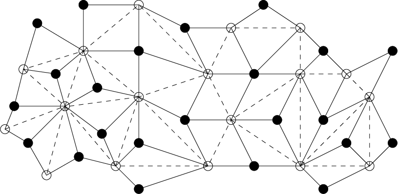
In particular, assume we are given a cell decomposition $\mathscr{K}$ of (a part of) $\mathbb{C}$ into kites. More precisely, $\mathscr{K}$ is a strongly regular cell decomposition whose 2-cells (faces) are embedded quadrilaterals (in fact kites), that is, there are exactly four edges incident to each face, with counterclockwise orientation. Furthermore, we assume that the 1-skeleton of $\mathscr{K}$ is a bipartite graph whose edges are straight line segments and that the vertices are colored white and black as in Figure 1 (left). For every white vertex we suppose that the lengths of the incident egdes agree as in Figure 1 (right) and add a circle with center at this vertex which passes through the incident black vertices of $\mathscr{K}$ . So white vertices correspond to centers of circles and black vertices correspond to intersection points. An example is illustrated in Figure 1 (right). This leads to an embedded planar circle pattern $\mathscr{C}$ . Obviously, the combinatorics of this circle pattern is described by the combinatorics of $\mathscr{K}$ . Furthermore, we can read off the (exterior) intersection angles $\alpha$ between the circles, as illustrated in Figure 2 (left). We associate this intersection angle to the kites of $\mathscr{K}$ .

Figure 1. Left: An example of a b-quad-graph

\mathscr{D}

(black edges, quadrilateral faces and bicolored vertices); right: A corresponding circle pattern

\mathscr{C}

for

\mathscr{D}

with indicated kite pattern

\mathscr{K}

isomorphic to

\mathscr{D}

, one of the kites is colored

As we are interested in different circle patterns with the same combinatorics and the same intersection angles, we describe the combinatorics using an abstract strongly regular cell decomposition $\mathscr{D}$ of (a part of) $\mathbb{C}$ which may be realized as a cell decomposition $\mathscr{K}$ with kites. The set of faces of $\mathscr{D}$ is denoted by $F({\mathscr{D}})$ . We always assume that the 1-skeleton of $\mathscr{D}$ is a bipartite graph and that the vertices are colored white and black as in Figure 1 (left). Such a cell decomposition $\mathscr{D}$ will be called b-quad-graph. We are interested in planar embedded circle patterns $\mathscr{C}$ for a given b-quad-graph $\mathscr{D}$ which means that the combinatorics of the corresponding kite pattern $\mathscr{K}$ is isomorphic to $\mathscr{D}$ . In this article, we only consider embedded circle patterns, that is, different kites have mutually disjoint interiors. Therefore, we sometimes identify (the abstract cell decomposition) $\mathscr{D}$ with the kite pattern $\mathscr{K}$ and we will frequently omit the word ‘embedded’.

To the quadrilateral faces of a b-quad graph $\mathscr{D}$ we associate a function $\alpha:F({\mathscr{D}})\to(0,\pi)$ , called labelling. Given an embedded circle pattern $\mathscr{C}$ for $\mathscr{D}$ and the corresponding pattern of kites $\mathscr{K}$ , we can read off for every kite the (exterior) intersection angle between the circles, as illustrated in Figure 2 (left), and compare this to the value $\alpha(f)$ for the corresponding face $f$ of $\mathscr{D}$ . If all these values agree, then $\mathscr{C}$ is called a circle pattern for $\mathscr{D}$ and $\alpha$ . Note that we only consider planar circle patterns and will therefore omit the notion ‘planar’ in the following. But planarity of the circle pattern implies that the intersection angles at an interior black vertex sum up to $2\pi$ . Therefore, we demand as a necessary condition for the labelling $\alpha$ that at all interior black vertices $v$ we have

\sum_{f\text{ incident to }v}\alpha(f)=2\pi.

(1)

Such a labelling $\alpha$ of the faces will be called admissible.

Figure 2. Left: The exterior intersection angle

\alpha

of two intersecting circles and the associated kite built from centers and intersection points; right: An example of a circle packing (black circles) with additional circles (dashed) added to obtain an orthogonal circle pattern

Circle patterns for given combinatorics and intersection angles have been introduced and studied for example in [Sch92, BS93, Riv94, Sch97, BS04]. We recall some results in Section 2. Moreover, circle patterns generalize planar circle packings which are configurations of discs corresponding to a triangulation of a planar domain where vertices correspond to discs and for each edge the two corresponding discs touch. Every such circle packing can be understood as an orthogonal circle pattern by adding circles corresponding to the triangular faces through the three touching points, see Figure 2 (right) for an example. The corresponding intersection angles are all $\pi/2$ . More details can for example be found in the monograph [Ste05] and in the references therein.

Our first question in this article concerns a discrete analogue of Liouville’s theorem in complex analysis, that is “Any bounded entire function is constant”. To this end, we investigate infinite circle patterns whose corresponding kite patterns fill the whole complex plane $\mathbb{C}$ or the unit disc $\mathbb{D}$ . Obviously, the underlying b-quad-graph is also infinite. We always assume that these infinite circle patterns are locally finite in $\mathbb{C}$ or $\mathbb{D}$ , that is, for every compact subset of $\mathbb{C}$ or $\mathbb{D}$ , respectively, there are only finitely many kites of the corresponding kite pattern which intersect this set.

For such infinite circle patterns, rigidity of these configurations is a natural question. In particular, given two infinite locally finite embedded circle patterns ${\mathscr{C}}$ and $\widetilde{\mathscr{C}}$ with the same combinatorics and the same intersection angles, they should be related by an Euclidean similarity in $\mathbb{C}$ or a hyperbolic isometry in $\mathbb{D}$ , respectively. In [He99], He proved rigidity for infinite embedded locally finite Thurston-type circle patterns with exterior intersection angles in $[\pi/2,\pi]$ . These are patterns where circles correspond to vertices of a triangulation and for each edge the two corresponding circles intersect with given exterior intersection angles (with an additional condition for the case $\alpha(f)=\pi/2$ ). Note that Thurston-type circle patterns are in general not circle patterns with respect to our definition used in this paper, but some special classes of circle patterns are included. In particular, He’s result holds for orthogonal circle patterns, that is circle patterns as defined above with $\alpha\equiv\pi/2$ . Adapting ideas of He’s proof, we show that rigidity holds for locally finite circle patterns in $\mathbb{D}$ without restrictions on intersection angles.

Theorem 1.1 (Rigidity of infinite circle patterns in the hyperbolic disc).

Let $\mathscr{D}$ be a b-quad-graph and let $\alpha:F({\mathscr{D}})\to(0,\pi)$ be an admissible labelling. Let ${\mathscr{C}}$ and $\widetilde{\mathscr{C}}$ be two locally finite embedded infinite circle patterns for $\mathscr{D}$ and $\alpha$ which are contained in $\mathbb{D}$ . Assume that the kites of the corresponding kite patterns ${\mathscr{K}}$ and $\widetilde{\mathscr{K}}$ cover the whole unit disc $\mathbb{D}$ in each case. Then there is a hyperbolic isometry $f:\mathbb{D}\to\mathbb{D}$ such that $\widetilde{\mathscr{C}}=f({\mathscr{C}})$ .

The proof relies on a generalized maximum principle for the radius function of the circle pattern in the hyperbolic disc which is shown in Section 3.

For infinite circle patterns covering the whole complex plane we adapt further ideas of He [He99] and prove rigidity for the class of infinite circle patterns whose intersection angles are uniformly bounded from below.

Theorem 1.2 (Rigidity of infinite Euclidean circle patterns).

Let $\mathscr{D}$ be a b-quad-graph, $\alpha_{0}\in(0,\pi/2]$ and let $\alpha:F({\mathscr{D}})\to(\alpha_{0},\pi)$ be an admissible labelling. Let ${\mathscr{C}}$ and $\widetilde{\mathscr{C}}$ be two locally finite embedded infinite circle patterns for $\mathscr{D}$ and $\alpha$ . Assume that the kites of the corresponding kite patterns ${\mathscr{K}}$ and $\widetilde{\mathscr{K}}$ cover the whole plane $\mathbb{C}$ in each case. Then there is a Euclidean similarity $f:\mathbb{C}\to\mathbb{C}$ such that $\widetilde{\mathscr{C}}=f({\mathscr{C}})$ .

The proof is given in Section 4. Some parts of the proof rely heavily on estimates using vertex extremal length for graphs. This notion and some properties are introduced in Section 5.

Recall that smooth conformal maps preserve intersection angles. Therefore, pairs of circle patterns with the same combinatorics may be considered as discrete analogues of smooth conformal maps if all corresponding interesection angles agree. More precisely, we consider a piecewise linear map between two kite patterns corresponding to (finite) embedded circle patterns as a discrete conformal map.

Definition 1.3.

Let ${\mathscr{C}}$ and $\widetilde{\mathscr{C}}$ be two embedded circle patterns with the same combinatorics and the same intersection angles. Let ${\mathscr{K}}$ and $\widetilde{\mathscr{K}}$ be the corresponding kite patterns. Split every kite of these patterns into two triangles along the symmetry axis which connects its two white vertices. Define a global homeomorphism $f^{\Diamond}:{\mathscr{K}}\to\widetilde{\mathscr{K}}$ by the condition that the restriction of $f^{\Diamond}$ to each such triangle of ${\mathscr{K}}$ is an affine-linear map onto the corresponding triangle of $\widetilde{\mathscr{K}}$ . In particular, $f^{\Diamond}$ maps black and white vertices of ${\mathscr{K}}$ to corresponding points of $\widetilde{\mathscr{K}}$ . By abuse of notation we also denote this discrete conformal map as $f^{\Diamond}:{\mathscr{C}}\to\widetilde{\mathscr{C}}$ .

The second aim of this article is to study some sequences of discrete conformal maps and show that they approximate smooth conformal maps.

The convergence of discrete conformal maps based on circle packings was first conjectured by Thurston [Thu85] and then proven for regular hexagonal combinatorics, see [RS87, HS98]. Furthermore, He and Schramm studied in [HS96] the approximation of a conformal homeomorphism by circle packings with arbitrary combinatorics.

Circle patterns with the combinatorics of the square grid and their relations to smooth conformal maps have been studied in [Sch97, Mat05, LD07]. These regular circle patterns form a special case of isoradial circle patterns where all circles have the same radius. For isoradial circle patterns with uniformly bounded intersection angles convergence has been shown in [Büc08]. Using ideas from [HS96] and [RS87], we prove in this article convergence to a conformal map for the class of q-bounded convex circle patterns. These circle patterns satisfy the condition that all kites are convex and the quotients of lengths of the diagonals of the kites are uniformly bounded in $[1/q,q]$ , see Definition 6.1. In particular, we obtain the following result.

Theorem 1.4.

Let $D$ and $\widetilde{D}$ be two simply connected bounded domains in $\mathbb{C}$ . Let $p_{0}\in D$ be some ‘reference’ point. Let $({\mathscr{D}}_{n})_{n\in\mathbb{N}}$ be a sequence of finite b-quad-graphs which are cell decompositions of a topological closed disc.

Let $q>1$ . For every $n\in\mathbb{N}$ assume that ${\mathscr{C}}_{n}$ and $\widetilde{\mathscr{C}}_{n}$ are two embedded convex q-bounded circle patterns for ${\mathscr{D}}_{n}$ and some admissible labelling $\alpha_{n}$ whose kites all lie in $D$ and $\widetilde{D}$ respectively.

Let $(\delta_{n})_{n\in\mathbb{N}}$ be a sequence of positive numbers such that $\delta_{n}\searrow 0$ for $n\to\infty$ . For each $n\in\mathbb{N}$ denote by $r_{n}(v)$ the radius of the circle in ${\mathscr{C}}_{n}$ for the white vertex $v$ and assume that $r_{n}(v)<\delta_{n}/2$ for all white vertices. Suppose further that the Euclidean distance of the subset covered by the kites of ${\mathscr{C}}_{n}$ to the boundary $\partial D$ is smaller than $\delta_{n}$ , i.e. $d({\mathscr{S}}_{n},\partial D)<\delta_{n}$ where ${\mathscr{S}}_{n}$ is the union of all kites of ${\mathscr{K}}_{n}$ , and also $d(\widetilde{\mathscr{S}}_{n},\partial\widetilde{D})<\delta_{n}$ where $\widetilde{\mathscr{S}}_{n}$ is the union of all kites of $\widetilde{\mathscr{K}}_{n}$ . Finally, let $p_{0}$ be covered by a kite for every $n\in\mathbb{N}$ and let the closure of the image points $\overline{(f_{n}^{\Diamond}(p_{0}))}_{n\in\mathbb{N}}$ be compact in $\widetilde{D}$ .

Then a subsequence of $(f_{n}^{\Diamond})_{n\in\mathbb{N}}$ converges uniformly on compact subsets of $D$ to a conformal homeomorphism $f:D\to\widetilde{D}$ .

The proof is presented in Section 6 and also relies on the generalized maximum principle for the radius function in Section 3 and on topological properties studied in Section 5.2.

Note that convergence issues on q-bounded kite patterns for Dirichlet problems with respect to the linear Laplacian (see (24) below) have recently been investigated in [Wer15].

2. Some properties of circle patterns

We start by introducing some useful notations.

Recall that the combinatorics for a circle pattern is given via a b-quad-graph $\mathscr{D}$ , that is a strongly regular cell decomposition of (a part of) $\mathbb{C}$ whose 2-cells (faces) are embedded quadrilaterals (respecting the counterclockwise orientation of $\mathbb{C}$ ), so in particular there are exactly four edges incident to each face. Moreover, its 1-skeleton is a bipartite graph with bicolored vertices. It is called simply connected if it is the cell decomposition of a simply connected domain of $\mathbb{C}$ . The two sets of vertices (colored white and black respectively) give rise to two planar graphs $G$ and $G^{*}$ as follows. The vertices $V(G)$ are all white vertices of $V(\mathscr{D})$ and correspond to centers of circles. The edges $E(G)$ correspond to faces of $\mathscr{D}$ , that is two vertices of $G$ are connected by an edge if and only if they are incident to the same face of $\mathscr{D}$ , see Figure 3.

Refer to caption — Figure 3. An example of a b-quad-graph $\mathscr{D}$ (black edges and bicolored vertices) and its associated graph $G$ (dashed edges and white vertices)

We denote by $V_{\text{int}}(G)$ the set of interior vertices of $G$ and by $V_{\partial}(G)$ the set of boundary vertices. The dual graph $G^{*}$ is constructed analogously by taking for $V(G^{*})$ all black vertices of $V(\mathscr{D})$ which correspond to intersection points. Faces of $\mathscr{D}$ or edges of $G$ or $G^{*}$ correspond to kites of intersecting circles. Furthermore, by abuse of notation, every labelling $\alpha:F({\mathscr{D}})\to(0,\pi)$ of the faces of $\mathscr{D}$ can also be understood as a function defined on the edges $E(G)$ or $E(G^{*})$ . We denote the value of this function by $\alpha(f)$ or $\alpha_{e}$ .

In this article we are concerned with embedded circle patterns. Nevertheless, some useful properties naturally include the more general case of immersed circle patterns.

Definition 2.1.

Let $\mathscr{D}$ be a b-quad-graph and let $\alpha:E(G)\to(0,\pi)$ be an admissible labelling. An immersed circle pattern for $\mathscr{D}$ (or $G$ ) and $\alpha$ is an indexed collection ${\mathscr{C}}=\{{\mathscr{C}}(v):v\in V(G)\}$ of circles in $\mathbb{C}$ and an indexed collection ${\mathscr{K}}=\{K_{e}=K(e):e\in E(G)\}$ of closed kites, which all carry the same orientation, such that the following conditions hold.

(1)

If $v_{1},v_{2}\in V(G)$ are incident vertices in $G$ , the corresponding circles ${\mathscr{C}}(v_{1}),{\mathscr{C}}(v_{2})$ intersect with exterior intersection angle $\alpha_{[v_{1},v_{2}]}$ . Furthermore, the kite $K_{[v_{1},v_{2}]}$ is bounded by the centers of the circles ${\mathscr{C}}(v_{1}),{\mathscr{C}}(v_{2})$ , the two intersection points, and the corresponding edges, as in Figure 2 (left). The intersection points are associated to black vertices of $V(\mathscr{D})$ or to vertices of $V(G^{*})$ .
(2)

The kite pattern is locally isomorphic to the b-quad-graph $\mathscr{D}$ at every interior vertex.

There are also other definitions for circle patterns, for example associated to a Delaunay decomposition of a domain in $\mathbb{C}$ for a given set of points (=vertices). This is a cell decomposition such that the boundary of each face is a polygon with straight edges which is inscribed in a circular disk, and these disks have no vertices in their interior. The corresponding embedded circle pattern can be associated to the graph $G^{*}$ . The Poincaré-dual decomposition of a Delaunay decomposition with the centers of the circles as vertices and straight edges is a Dirichlet decomposition (or Voronoi diagram) and corresponds to the graph $G$ .

Furthermore the definition of immersed circle patterns can be extended allowing cone-like singularities in the vertices; see [BS04] and the references therein.

Our study of a planar circle pattern ${\mathscr{C}}$ is based on characterizations and properties of its radius function $r_{\mathscr{C}}=r$ which assigns to every vertex $z\in V(G)$ the radius $r_{\mathscr{C}}(z)=r(z)$ of the corresponding circle ${\mathscr{C}}(z)$ . The index $\mathscr{C}$ will be dropped whenever there is no confusion likely.

The following proposition specifies a necessary and sufficient condition for a radius function to originate from a planar circle pattern, see also [BS04]. For the special case of orthogonal circle patterns with the combinatorics of the square grid, there are also other characterizations, see for example [Sch97].

Proposition 2.2.

Let $G$ be a graph constructed from a b-quad-graph $\mathscr{D}$ and let $\alpha$ be an admissible labelling.

Suppose that ${\mathscr{C}}$ is an immersed circle pattern for ${\mathscr{D}}$ and $\alpha$ with radius function $r=r_{\mathscr{C}}$ . Then for every interior vertex $v_{0}\in V_{int}(G)$ we have

\Biggl(\sum_{[v,v_{0}]\in E(G)}f_{\alpha_{[v,v_{0}]}}(\log r(v)-\log r(v_{0}))\Biggr)-\pi=0,

(2)

where

f_{\theta}(x):=\frac{1}{2i}\log\frac{1-e^{x-i\theta}}{1-e^{x+i\theta}},

(3)

and the branch of the logarithm is chosen such that $0<f_{\theta}(x)<\pi$ .

Conversely, suppose that $\mathscr{D}$ is simply connected and that $r:V(G)\to(0,\infty)$ satisfies (2) for every $v\in V_{int}(G)$ . Then there is an immersed circle pattern for $G$ and $\alpha$ whose radius function coincides with $r$ . This pattern is unique up to isometries of $\mathbb{C}$ .

Note that $2f_{\alpha_{[v,v_{0}]}}(\log r(v)-\log r(v_{0}))$ is the angle at $v_{0}$ of the kite with edge lengths $r(v)$ and $r(v_{0})$ and angle $\alpha_{[v,v_{0}]}$ , as in Figure 2 (left). Equation (2) is the closing condition for the chain of kites corresponding to the edges incident to $v_{0}$ .

Proof.

The statements are shown in a more general context in [BS04, Section 3] in the case of finite circle patterns. As (2) is only a local condition, it still holds for infinite patterns.

Also, given any radius function for the simply connected b-quad-graph $\mathscr{D}$ and the admissible labelling $\alpha$ , we can subsequently construct a corresponding circle pattern. For each quad with white vertices $v_{1}$ and $v_{2}$ build a kite as in Figure 2 (left) with sides of lengths $r(v_{1})$ and $r(v_{2})$ and angle $\alpha_{[v_{1},v_{2}]}$ opposite to the symmetry axis of the kite. Because corresponding sides have the same length, these kites may be glued together to form a cellular decomposition equivalent to $\mathscr{D}$ . Condition (2) and the admissible labelling assure that the resulting kite pattern can locally be embedded in the plane. Also, we obtain by construction a corresponding circle pattern if we add circles of radius $r(v)$ through all vertices of the kites which correspond to black vertices incident to $v$ in $\mathscr{D}$ . In particular, we can start with any kite corresponding to a face $f$ of $\mathscr{D}$ and embed it into the plane. This fixes the rotational and translational freedom. Then we glue kites for faces adjacent to $f$ and successively proceed. Due to our assumptions on the labelling and to condition (2), the (finite) chain of kites corresponding to the edges incident to any fixed vertex will close up. Proceeding in this way for all faces of the simply connected b-quad-graph $\mathscr{D}$ finally leads to an immersed (maybe infinite) circle pattern.

∎

For further use we mention some properties of $f_{\theta}$ , see for example [Spr03].

Lemma 2.3.

(1)

The derivative of $f_{\theta}$ is $f_{\theta}^{\prime}(x)=\frac{\sin\theta}{2(\cosh x-\cos\theta)}>0$ . So $f_{\theta}$ is strictly increasing.
(2)

The function $f_{\theta}$ satisfies the functional equation $f_{\theta}(x)+f_{\theta}(-x)=\pi-\theta$ .
(3)

For $0<y<\pi-\theta$ the inverse function of $f_{\theta}$ is $f_{\theta}^{-1}(y)=\log\frac{\sin y}{\sin(y+\theta)}$ .
(4)

The integral of $f_{\theta}$ is

$F_{\theta}(x)=\int_{-\infty}^{x}f_{\theta}(\xi)d\xi=\mathrm{Im}\;\mathrm{Li}_{2}(e^{x+i\theta}),$

where $\;\mathrm{Li}_{2}(z)=-\int_{0}^{z}\frac{\log(1-\zeta)}{\zeta}d\zeta$ is the dilogarithm function, see for example [Lew81].

In analogy to smooth harmonic functions, the radius function of a planar circle pattern satisfies a Dirichlet principle and a maximum principle.

Theorem 2.4 (Dirichlet Principle).

Let $G$ be a graph constructed from a finite simply connected b-quad-graph $\mathscr{D}$ and let $\alpha$ be an admissible labelling.

Let $r:V_{\partial}(G)\to(0,\infty)$ be some positive function on the boundary vertices of $G$ . Then $r$ can be extended to $V(G)$ in such a way that equation (2) holds at every interior vertex $z\in V_{int}(G)$ if and only if there exists any immersed circle pattern for $G$ and $\alpha$ . If it exists, the extension is unique.

See for example [Büc08, Theorem 2.6] for a proof.

Lemma 2.5 (Maximum Principle).

Let $G$ be a graph constructed from a b-quad-graph $\mathscr{D}$ and let $\alpha$ be an admissible labelling. Suppose ${\mathscr{C}}$ and $\widetilde{\mathscr{C}}$ are two immersed circle patterns for $G$ and $\alpha$ with radius functions $r$ and $\tilde{r}$ resp. Then the maximum (or minimum) of the quotient $r/\tilde{r}$ is attained at a boundary vertex.

A proof can be found in [He99, Lemma 2.1]. If there exists an isoradial planar circle pattern for $G$ and $\alpha$ , the usual maximum principle for the radius function follows by taking $\tilde{r}\equiv 1$ .

3. Maximum principles and rigidity of circle patterns in the hyperbolic plane

For a circle pattern $\mathscr{C}$ in the unit disc $\mathbb{D}$ for the graph $G$ denote by $r_{\text{hyp}}:V(G)\to\mathbb{R}$ the function which assigns to each vertex the hyperbolic radius of the corresponding circle.

Lemma 3.1 (Maximum Principle in the hyperbolic plane).

Let $G$ be a graph constructed from a b-quad-graph $\mathscr{D}$ and let $\alpha$ be an admissible labelling. Let ${\mathscr{C}}$ and ${\mathscr{C}}^{*}$ be two circle patterns for $G$ and $\alpha$ which are contained in $\mathbb{D}$ .

If the inequality $r_{\text{hyp}}^{*}(v)\geq r_{\text{hyp}}(v)$ is satisfied for each boundary vertex, then it holds for all vertices of $G$ .

Our proof is based on a variational principle for circle patterns by Springborn and Bobenko, see [BS04, Spr03]. We will briefly present some useful facts.

First we introduce some notation. For a hyperbolic circle pattern for $G$ denote by $c_{\text{hyp}}:V(G)\to\mathbb{C}$ the function assigning the hyperbolic center of circle to the vertex of the corresponding circle. Also, instead of the hyperbolic radius function $r_{\text{hyp}}$ we will often consider the function

\rho:V(G)\to\mathbb{R},\qquad\rho(v)=\log\tanh\frac{r_{\text{hyp}}(v)}{2}.

(4)

Note that positive hyperbolic radii $r_{\text{hyp}}(v)$ correspond to negative $\rho(v)$ .

Consider two intersecting circles in $\mathbb{D}$ corresponding to the edge $e=[v_{0},v_{1}]$ . Let $\alpha_{e}=\theta\in(0,\pi)$ be the exterior intersection angle of the two circles ${\mathscr{C}}(v_{0})$ and ${\mathscr{C}}(v_{1})$ . Consider the hyperbolic triangle formed by the two centers $c_{\text{hyp}}(v_{0})$ and $c_{\text{hyp}}(v_{1})$ and one of the intersection points of the two circles, see Figure 4 for a schematic sketch. Then the angle at $c_{\text{hyp}}(v_{0})$ in this triangle is

\varphi_{e}(\rho(v_{0}),\rho(v_{1}),\theta)=f_{\theta}(\rho(v_{1})-\rho(v_{0}))-f_{\theta}(\rho(v_{1})+\rho(v_{0})),

(5)

where the function $f_{\theta}:\mathbb{R}\to\mathbb{R}$ is defined in (3).

(a) Definition of the angle

\varphi_{e}=\varphi_{e}(\rho(v_{0}),\rho(v_{1}),\theta)

in a hyperbolic triangle (schematic drawing, all lines are geodesics)

(b) Generalization of

\varphi_{e}

\varphi_{e}^{g}

(schematic drawing, bold lines are geodesics)

Figure 4. Definition of the angle functions for (generalized) hyperbolic circle patterns.

In a planar (hyperbolic) circle pattern these angles $\varphi_{e}$ add up to $\pi$ around an interior vertex $v_{0}$ . Therefore we have analogously as in Proposition 2.2 the following characterization of hyperbolic circle patterns.

Proposition 3.2 ([BS04, Spr03]).

Let $G$ be a graph constructed from a b-quad-graph $\mathscr{D}$ and let $\alpha$ be an admissible labelling.

(i)

Suppose that ${\mathscr{C}}$ is a planar hyperbolic circle pattern for ${\mathscr{D}}$ and $\alpha$ with hyperbolic radius function $r=r_{\text{hyp}}$ and $\rho=\log\tanh\frac{r_{\text{hyp}}}{2}$ . Then for every interior vertex $v_{0}\in V_{int}(G)$ we have

2\pi-2\sum_{[v_{0},v]\in E(G)}(f_{\alpha_{[v_{0},v]}}(\rho(v)-\rho(v_{0}))-f_{\alpha_{[v_{0},v]}}(\rho(v)+\rho(v_{0})))=0.

(6)

(ii)

Conversely, suppose that $\mathscr{D}$ is simply connected and assume that the variables $\rho=\log\tanh\frac{r}{2}\in(-\infty,0)$ for a hyperbolic radius function $r:V(G)\to(0,\infty)$ satisfy (2) for every $v_{0}\in V_{int}(G)$ . Then there is a planar hyperbolic circle pattern for $G$ and $\alpha$ whose hyperbolic radius function coincides with $r$ . This pattern is unique up to isometries of $\mathbb{D}$ .

(iii)

For given boundary values $\rho:V_{\partial}(G)\to(-\infty,0)$ there exists a unique solution $\rho:V_{\text{int}}(G)\to\mathbb{R}$ of equations (6) which is the minimizer of the strictly convex functional $S_{\text{hyp}}:\mathbb{R}^{N}\to\mathbb{R}$ , where $N=|V_{int}(G)|$ and

S_{\text{hyp}}(\rho)=\sum_{e=[v_{l},v_{r}]}\left(\mathrm{Im}\;\mathrm{Li}_{2}(e^{\rho(v_{l})-\rho(v_{r})+i\alpha_{e}})+\mathrm{Im}\;\mathrm{Li}_{2}(e^{\rho(v_{r})-\rho(v_{l})+i\alpha_{e}})\right.\\ \left.+\mathrm{Im}\;\mathrm{Li}_{2}(e^{\rho(v_{l})+\rho(v_{r})+i\alpha_{e}})+\mathrm{Im}\;\mathrm{Li}_{2}(e^{-\rho(v_{l})-\rho(v_{r})+i\alpha_{e}})\right)\\ +\sum_{v\in V_{int}(G)}2\pi\rho(v).

(7)

The first sum is taken over all edges $e\in E(G)$ .

Note in particular that for all $v_{0}\in V_{int}(G)$ and $\rho_{0}=\rho(v_{0})$ we have

\frac{\partial S_{\text{hyp}}(\rho)}{\partial\rho_{0}}=2\pi-2\sum_{[v_{0},v]\in E(G)}(f_{\alpha_{[v_{0},v]}}(\rho(v)-\rho(v_{0}))-f_{\alpha_{[v_{0},v]}}(\rho(v)+\rho(v_{0}))).

Remark 3.3.

The statements of the preceding proposition can be generalized to hyperbolic circle patterns with cone singularities at the vertices, see [BS04, Spr03].

Now we are ready to prove the Maximum Principle in the hyperbolic plane.

of Lemma 3.1.

First note that $\rho(r)=\log\tanh\frac{r}{2}$ is strictly monotonically increasing in (the hyperbolic radius) $r$ .

By Proposition 3.2, circle patterns in $\mathbb{D}$ correspond uniquely to critical points of the functional $S_{\text{hyp}}$ . Furthermore, $S_{\text{hyp}}$ is strictly convex and its unique critical point is a minimum.

Let $v_{1},\dots,v_{n}$ be a numbering of the interior vertices of $G$ where $n=|V_{int}(G)|$ . Let $\rho,\rho^{*}:V(G)\to(-\infty,0)$ correspond to the radii as above. Consider in $\mathbb{R}^{n}$ the $n$ -dimensional closed interval $U=\{u\in\mathbb{R}^{n}\ |\ u_{i}\leq\rho^{*}(v_{i})\}$ . We will show that for fixed boundary values $\rho|_{\partial V}$ the gradient of $S_{\text{hyp}}(\cdot,\rho|_{\partial V}):\mathbb{R}^{n}\to\mathbb{R}$ is pointing into the complement of $U$ on the boundary $\partial U$ or is contained in $\partial U$ (or more precisely in one of the hyperplanes $H_{i}=\{u\in\mathbb{R}^{n}\ |\ u_{i}=\rho^{*}(v_{i})\}$ ).

For $u_{i}=\rho^{*}(v_{i})$ the $i$ th component of the gradient of $S_{\text{hyp}}$ is

\frac{\partial S_{\text{hyp}}(\rho)}{\partial u_{i}}(u_{1},\dots,u_{i}=\rho^{*}(v_{i}),\dots u_{n})\\ =2\pi-2\sum_{[v_{i},v_{k}]\in E(G)}(f_{\alpha_{[v_{i},v_{k}]}}(u_{k}-\rho^{*}(v_{i}))-f_{\alpha_{[v_{i},v_{k}]}}(u_{k}+\rho(v_{i})))\\ \geq 2\pi-2\sum_{[v_{i},v_{k}]\in E(G)}(f_{\alpha_{[v_{i},v_{k}]}}(\rho^{*}(v_{k})-\rho^{*}(v_{i}))-f_{\alpha_{[v_{i},v_{k}]}}(\rho^{*}(v_{k})+\rho(v_{i})))\\ \qquad=\frac{\partial S_{\text{hyp}}(\rho)}{\partial u_{i}}(\rho^{*}(v_{1}),\dots,\rho^{*}(v_{n}))=0.

The sum is taken over all edges $[v_{i},v_{k}]\in E(G)$ incident to $v_{i}$ . The inequality follows from the fact that

	$\displaystyle\frac{\partial}{\partial u_{k}}\varphi_{e}(u_{i},u_{k},\theta)$	$\displaystyle=\frac{\partial}{\partial u_{k}}(f_{\theta}(u_{k}-u_{i})-f_{\theta}(u_{k}+u_{i}))$
		$\displaystyle=\frac{\sin\theta}{2(\cosh(u_{k}-u_{i})-\cos\theta)}-\frac{\sin\theta}{2(\cosh(u_{k}+u_{i})-\cos\theta)}>0.$

Furthermore the inequality is strict if at least for one edge $[v_{i},v_{k}]\in E(G)$ we have a strict inequality $u_{k}<\rho^{*}(v_{k})$ . Therefore the minimum of $S_{\text{hyp}}$ with boundary conditions $\rho|_{\partial V}$ in contained in $U$ . ∎

Similarly as He in [He99] we now generalize this maximum principle to circle patterns which only intersect the unit disc $\mathbb{D}$ . For this reason, we generalize the hyperbolic functional $S_{\text{hyp}}$ for circles intersecting the boundary $\partial\mathbb{D}$ .

Remark 3.4.

In the Poincaré disc model of the hyperbolic geometry the geodesics are the intersections of circles orthogonal to $\partial\mathbb{D}$ with $\mathbb{D}$ . Consider a circle which intersects $\partial\mathbb{D}$ in two points with exterior intersection angle $\beta$ . Then all points on the corresponding circular arc in $\mathbb{D}$ have the same distance to one fixed geodesic which intersects $\partial\mathbb{D}$ in the same two points, see Figure 5. This distance $\delta$ satisfies

\displaystyle i\beta=\log\tanh\left(\frac{\delta}{2}+i\frac{\pi}{4}\right).

(8)

These curves are also called hypercycles and may be interpreted as generalization of circles where all points have the same distance to one fixed point (which is the center).

Figure 5. A circular arc corresponding to a hypercycle in the Poincaré disc model with exterior intersection angle

\beta

and distance

\delta

to the corresponding geodesic (dashed line).

First, we generalize the angle function $\varphi_{e}$ . Consider a circular arc intersecting $\partial\mathbb{D}$ in some exterior angle $\beta\in[0,\pi)$ which intersects a circle contained in $\mathbb{D}$ in an angle $\theta\in(0,\pi)$ . Let $c=c_{\text{hyp}}$ be the center of this circle and $r=r_{\text{hyp}}$ its radius. Set $\rho=\log\tanh\frac{r}{2}$ as above. Then the angle $\varphi_{e}^{g}(\rho,\beta,\theta)$ at $c$ is given by (see Figure 4):

	$\displaystyle\varphi_{e}^{g}(\rho,\beta,\theta)$	$\displaystyle=\frac{1}{2i}\log\left(\frac{\cos\beta-\cosh(\rho+i\theta)}{\cos\beta-\cosh(\rho-i\theta)}\right)$		(9)
		$\displaystyle=f_{\theta}(i\beta-\rho)-f_{\theta}(i\beta+\rho)$		(10)

In the first equation, the logarithm is chosen such that $\varphi_{e}^{g}\in(0,\pi)$ . For the second equation we use a suitable generalization (in fact extention) of the function $f_{\theta}$ which maps $D_{\theta}=\mathbb{R}\times(-i\pi,i\pi)\setminus B_{\theta}$ with $B_{\theta}=\{0\}\times(-i\pi,-i\theta]\cup\{0\}\times[i\theta,i\pi)$ to a simply connected domain in $\{x+iy\ :\ x\in(-\frac{\theta}{2},\pi-\frac{\theta}{2}),\ y\in\mathbb{R}\}\subset\mathbb{C}$ .

Note that there is an analogous formula for the distance $\delta$ , namely

	$\displaystyle-i\delta$	$\displaystyle=\frac{1}{2i}\log\left(\frac{\cosh\rho-\cos(\beta+\theta)}{\cosh\rho-\cos(\beta-\theta)}\right)$		(11)
		$\displaystyle=f_{\theta}(\rho-i\beta)-f_{\theta}(\rho+i\beta)$		(12)

Remark 3.5.

Note that $f_{\theta}$ is one-to-one on $D_{\theta}$ .

Furthermore we have for $\beta\in[0,\pi)$ :

		$\displaystyle\lim_{x\to-\infty}f_{\theta}(x\pm i\beta)=0,$		(13)
		$\displaystyle\lim_{x\to+\infty}f_{\theta}(x\pm i\beta)=\pi-\theta,$		(14)
		$\displaystyle f_{\theta}(x+i\beta)+f_{\theta}(-x-i\beta)=f_{\theta}(-x+i\beta)+f_{\theta}(x-i\beta)=\pi-\theta.$		(15)

Definition 3.6.

Let $G$ be a graph constructed from a b-quad-graph $\mathscr{D}$ and let $\alpha$ be an admissible labelling. Suppose that ${\mathscr{C}}$ is a planar Euclidean circle pattern for ${\mathscr{D}}$ and $\alpha$ such that all circles intersect the hyperbolic disc $\mathbb{D}$ . Then this circle pattern is called generalized hyperbolic circle pattern for ${\mathscr{D}}$ and $\alpha$ . To this circle pattern we associate a functional $\rho:V(G)\to\mathbb{C}$ which is $\rho(v)=\log\tanh\frac{r_{\text{hyp}}(v)}{2}$ for circles contained in $\mathbb{D}$ with hyperbolic radius $r_{\text{hyp}}(v)$ . For circles intersecting $\partial\mathbb{D}$ with exterior intersection angle $\beta\in[0,\pi)$ we set $\rho(v)=i\beta$ .

We immediately deduce from the definition of $\varphi_{e}^{g}$ in (10) the following generalization of Proposition 3.2 (i).

Proposition 3.7.

Let $G$ be a graph constructed from a b-quad-graph $\mathscr{D}$ and let $\alpha$ be an admissible labelling. Suppose that ${\mathscr{C}}$ is a generalized hyperbolic circle pattern for ${\mathscr{D}}$ and $\alpha$ with associated function $\rho$ . Then for every interior vertex $v_{0}\in V_{int}(G)$ we have

2\pi-2\sum_{[v_{0},v]\in E(G)}(f_{\alpha_{[v_{0},v]}}(\rho(v)-\rho(v_{0}))-f_{\alpha_{[v_{0},v]}}(\rho(v)+\rho(v_{0})))=0.

(16)

Now we generalize the hyperbolic functional $S_{\text{hyp}}$ . We only change the terms for all edges connecting an interior vertex of $G$ to a boundary vertex with intersection angle $\beta\in[0,\pi)$ . In other words, we change the term for edges where the function $\rho$ is real and negative on one vertex and purely imaginary or zero on the other vertex.

For $x\leq 0$ define

\displaystyle F_{\beta,\theta}(x)

\displaystyle:=2\int_{-\infty}^{x}(f_{\theta}(\eta+i\beta)+f_{\theta}(\eta-i\beta))d\eta-2(\pi-\theta)x.

For $x>0$ we set $F_{\beta,\theta}(x)=F_{\beta,\theta}(-x)$ .

There is a relation to the $\;\mathrm{Li}_{2}$ -function (at least for $\beta\not=\theta$ ) as in the finite case:

\int_{-\infty}^{x}f_{\theta}(\eta+i\beta)d\eta=\frac{1}{2i}(\;\mathrm{Li}_{2}(\text{e}^{x+i\beta+i\theta})-\;\mathrm{Li}_{2}(\text{e}^{x+i\beta-i\theta})).

By equation (15) we can write

	$\displaystyle-2(\pi-\theta)x$	$\displaystyle=\int_{x}^{0}(f_{\theta}(\eta+i\beta)+f_{\theta}(-\eta-i\beta)+f_{\theta}(\eta-i\beta)+f_{\theta}(-\eta+i\beta))d\eta$
		$\displaystyle=\int_{x}^{-x}f_{\theta}(\eta+i\beta)d\eta+\int_{x}^{-x}f_{\theta}(\eta-i\beta)d\eta.$

Thus we finally obtain

	$\displaystyle F_{\beta,\theta}(x)$	$\displaystyle=\frac{1}{2i}\left(\;\mathrm{Li}_{2}(\text{e}^{x+i\beta+i\theta})-\;\mathrm{Li}_{2}(\text{e}^{x+i\beta-i\theta})-\;\mathrm{Li}_{2}(\text{e}^{-x+i\beta-i\theta})+\;\mathrm{Li}_{2}(\text{e}^{-x+i\beta+i\theta})\right.$
		$\displaystyle\left.\quad+\;\mathrm{Li}_{2}(\text{e}^{x-i\beta+i\theta})-\;\mathrm{Li}_{2}(\text{e}^{x-i\beta-i\theta})-\;\mathrm{Li}_{2}(\text{e}^{-x-i\beta-i\theta})+\;\mathrm{Li}_{2}(\text{e}^{-x-i\beta+i\theta})\right).$

Moreover, we obtain again with (15)

	$\displaystyle\frac{\partial F_{\beta,\theta}}{\partial x}$	$\displaystyle=2(f_{\theta}(x+i\beta)+f_{\theta}(x-i\beta)-(\pi-\theta))=2(f_{\theta}(x+i\beta)-f_{\theta}(-x+i\beta))$
		$\displaystyle=-2\varphi^{g}(x,\beta,\theta).$

Now we are able to define the generalized hyperbolic functional $S_{\text{hyp}}^{g}(\rho)$ . First, let $V_{\partial,\beta}(G)$ be the set of boundary vertices which correspond to circles intersecting $\partial\mathbb{D}$ . Let $E_{\beta}(G)$ be the set of all edges which are incident to one interior vertex and one vertex of $V_{\partial,\beta}(G)$ . Let $n=|V_{int}(G)|$ , $k_{\beta}=|V_{\partial,\beta}(G)|$ and $k_{0}=|V_{\partial}(G)|-k_{\beta}$ . We define $S_{\text{hyp}}^{g}:\mathbb{R}^{n+k_{0}}\times(i\mathbb{R})^{k_{\beta}}\to\mathbb{R}$ similarly as in equation (7) as a sum over all edges. The summands are the same as above in (7) for all edges which are not incident to a vertex in $V_{\partial,\beta}(G)$ . Otherwise we take the summand $F_{\beta(v),\alpha_{[v,v_{0}]}}$ for edges $[v,v_{0}]$ with one interior vertex $v_{0}$ and the boundary vertex $v$ with exterior intersection angle $\beta(v)$ .

Note the following properties of $F_{\beta,\theta}$ .

(i)

	$\displaystyle\frac{\partial^{2}F_{\beta,\theta}}{\partial x^{2}}$	$\displaystyle=\frac{\sin\theta}{\cosh(x+i\beta)-\cos\theta}+\frac{\sin\theta}{\cosh(-x+i\beta)-\cos\theta}$
		$\displaystyle=\frac{2\sin\theta(\cosh x\cos\beta-\cos\theta)}{(\cosh x\cos\beta-\cos\theta)^{2}+(\sinh x\sin\beta)^{2}}.$

Thus for fixed boundary values $\rho|_{\partial V}$ (in particular for fixed $\beta(v)$ ) the functional $S_{\text{hyp}}^{g}$ is not necessarily convex.

(ii)

If for all edges $e=[v,v_{0}]\in E_{\beta}$ with $v\in V_{\partial,\beta}$ we have $\cos\alpha_{e}<\cos\beta(v)$ then $S_{\text{hyp}}^{g}$ is strictly convex and any critical point must be a minimum. In this case existence can be proven along the same lines as for the original function $S_{\text{hyp}}$ in [BS04, Spr03].

As an immediate consequence Proposition 3.7 can now be formulated as follows.

Corollary 3.8.

Then $\rho^{*}|_{V_{int}}$ is a critical point of the functional $S_{\text{hyp}}^{g}(\cdot,\rho^{*}|_{V_{\partial}})$ .

Furthermore, if for all interior edges $e$ incident to a vertex $v\in V_{\partial,\beta}$ the inequality $\cos\alpha_{e}<\cos\beta(v)$ holds, then this critical point is the unique minimizer of $S_{\text{hyp}}^{g}(\cdot,\rho^{*}|_{V_{\partial}})$ .

Finally, we can generalize the maximum principle 3.1.

Lemma 3.9 (Generalized Maximum Principle in the hyperbolic plane).

Let $G$ be a finite graph and let $\alpha:E(G)\to(0,\pi)$ be an admissible labelling. Let ${\mathscr{C}}$ be a circle pattern for $G$ and $\alpha$ which is contained in $\mathbb{D}$ . Let ${\mathscr{C}}^{*}$ be a generalized circle pattern for $G$ and $\alpha$ with exterior intersection angles $\beta:V_{\partial,\beta}(G)\to[0,\pi)$ . Suppose that for every boundary vertex either $v\in V_{\partial,\beta}(G)$ or the inequality $r_{\text{hyp}}^{*}(v)\geq r_{\text{hyp}}(v)$ holds. Then for all interior vertices $r_{\text{hyp}}^{*}(v)\geq r_{\text{hyp}}(v)$ .

Remark 3.10.

If $V_{\partial,\beta}(G)\not=\emptyset$ or if $r_{\text{hyp}}^{*}(v)>r_{\text{hyp}}(v)$ for one boundary vertex then the inequality is strict for all interior vertices.

Proof.

We suppose that $V_{\partial,\beta}(G)\not=\emptyset$ because the case $V_{\partial,\beta}(G)=\emptyset$ has be proven in Lemma 3.1. The idea of the proof is the same.

Let $v_{1},\dots,v_{n}$ be a numbering of the interior vertices of $G$ where $n=|V_{int}(G)|$ . Let $\rho$ and $\rho^{*}$ be the associated functions to ${\mathscr{C}}$ and ${\mathscr{C}}^{*}$ respectively as above. Recall that the circle pattern ${\mathscr{C}}$ is the unique minimizer of the strictly convex functional $S_{\text{hyp}}$ fixing the boundary values $\rho|_{V_{\partial}}$ . Consider in $\mathbb{R}^{n}$ the $n$ -dimensional interval $U=\{u\in\mathbb{R}^{n}\ :\ u_{i}<\rho^{*}(v_{i})\}$ . We will again show that for fixed boundary values $\rho|_{\partial V}$ the gradient of $S_{\text{hyp}}(\cdot,\rho|_{\partial V}):\mathbb{R}^{n}\to\mathbb{R}$ is pointing into the complement of $U$ on the boundary $\partial U$ or is contained in $\partial U$ (or in one of the hyperplanes $H_{i}=\{u\in\mathbb{R}^{n}\ |\ u_{i}=\rho^{*}(v_{i})\}$ ).

From the proof of Lemma 3.1 we know that if the vertex $v_{i}$ is not incident to any boundary vertex in $V_{\partial,\beta}(G)$ we have

\frac{\partial S_{\text{hyp}}(\rho)}{\partial u_{i}}(u_{1},\dots,u_{i}=\rho^{*}(v_{i}),\dots u_{n})\geq\frac{\partial S_{\text{hyp}}(\rho)}{\partial u_{i}}(\rho^{*}(v_{1}),\dots,\rho^{*}(v_{n}))=0,

(17)

where the sum is taken over all edges $[v_{i},v_{k}]\in E(G)$ incident to $v_{i}$ .

Note that

\frac{\partial\varphi^{g}_{e}}{\partial\beta}=-\frac{\sin\theta\sinh x\sin\beta}{|\cosh(x+i\beta)-\cos\theta|^{2}}>0

for $\beta>0$ and $x<0$ (and $=0$ for $\beta=0$ ). Recall that $\frac{\partial\varphi_{e}}{\partial u}(x,u,\theta)>0$ , therefore we deduce that

\varphi^{g}_{e}(x,\beta,\theta)\geq\varphi^{g}_{e}(x,0,\theta)=\lim_{u\nearrow 0}\varphi_{e}(x,u,\theta)>\varphi_{e}(x,u,\theta)

for all $x,u\in\mathbb{R}$ , $x,u<0$ . This implies as in the proof of Lemma 3.1 that estimate (17) holds for all vertices.

Thus the minimum is contained in $U$ . ∎

As an application we can deduce Theorem 1.1 with the same proof as for Theorem 1.2 in [He99].

4. Rigidity of infinite Euclidean circle patterns

In this section we show Theorem 1.2 on rigidity of infinite circle patterns in the plane. The proof adapts ideas and methods of He’s rigidity proof in [He99]. It mainly relies on the maximum principle in Lemma 3.9 and on estimates on vertex extremal length for patterns of circles explained in Section 5.

Let $\mathscr{D}$ , $\alpha$ , $\mathscr{C}$ and $\widetilde{\mathscr{C}}$ be as in Theorem 1.2. Let $G$ be the graph of white vertices associated to $\mathscr{D}$ . Let $r,\tilde{r}:V(G)\to(0,\infty)$ be the Euclidean radius functions of $\mathscr{C}$ and $\widetilde{\mathscr{C}}$ respectively.

The following lemma will be proved later in Appendix A.

Lemma 4.1.

Under the assumptions of Theorem 1.2 there is a constant $C\geq 1$ such that for every vertex $v\in V(G)$

\frac{1}{C}\leq\frac{\tilde{r}(v)}{r(v)}\leq C.

(18)

Assuming this lemma, we will first construct a one-parameter family of immersed circle patterns for $\mathscr{D}$ and $\alpha$ joining $\mathscr{C}$ and $\widetilde{\mathscr{C}}$ as follows. For every vertex $v\in V(G)$ denote $\lambda(v)=\log(\tilde{r}(v)/r(v))$ and define $\hat{r}(v,t):=\text{e}^{\lambda(v)t}r(v)$ . Then $\hat{r}(v,0)=r(v)$ , $\hat{r}(v,1)=\tilde{r}(v)$ and

\left|\log\frac{\hat{r}(v,t+\varepsilon)}{\hat{r}(v,t)}\right|=|\varepsilon||\lambda(v)|\leq|\varepsilon|\log C

(19)

for $t,t+\varepsilon\in[0,1]$ by (18).

Let $G_{n}$ be an increasing sequence of subgraphs of $G$ whose union is $G$ . We assume that $G_{n}$ is the associated graph of white vertices of a b-quad-graph ${\mathscr{D}}_{n}$ which is a cell decomposition of a closed topological disc. Then a subpattern of $\mathscr{C}$ is a circle pattern for $G_{n}$ and $\alpha|_{G_{n}}$ . By Theorem 2.4 and Proposition 2.2 for every $n$ and every $t\in[0,1]$ there exists an immersed circle pattern ${\mathscr{C}}_{n,t}$ for $G_{n}$ and $\alpha|_{G_{n}}$ with boundary values $r_{n,t}|_{\partial V(G_{n})}=\hat{r}(\cdot,t)|_{\partial V(G_{n})}$ . Lemma 2.5 together with estimate (19) implies that

\left|\log\frac{r_{n,t+\varepsilon}(v)}{r_{n,t}(v)}\right|\leq|\varepsilon|\log C

for any vertex $v\in V(G_{n})$ . Thus

\left|\frac{d}{dt}\log r_{n,t}(v)\right|\leq\log C.

(20)

Now, replacing by a suitable subsequence and applying Euclidean transformations if necessary, we may assume that for every vertex $v\in V(G)$ the sequence of circles ${\mathscr{C}}_{n,t}(v)$ converges in the Hausdorff metric to some limit circle ${\mathscr{C}}_{t}(v)$ . Then ${\mathscr{C}}_{t}$ is for every $t\in[0,1]$ an immersed circle pattern for $G$ and $\alpha$ . By the uniqueness part of Theorem 2.4 we may assume that ${\mathscr{C}}_{n,0}$ are subpatterns of ${\mathscr{C}}$ and therefore ${\mathscr{C}}_{0}=\mathscr{C}$ . Similarly we assume that ${\mathscr{C}}_{1}={\mathscr{C}}^{*}$ .

From estimate (19) we deduce

\left|\frac{d}{dt}\log r_{t}(v)\right|\leq\log C

(21)

where the derivative with respect to $t$ is taken in the generalized (distributional) sense. Let $\ell(v,t)=\log r_{t}(v)-\log r_{0}(v)$ . Then we have $\ell(v,0)=0$ and

\left|\frac{d}{dt}\ell(v,t)\right|\leq\log C

(22)

by (21). Let $t\in[0,1]$ be fixed. Define

h(v)=h(v,t)=\frac{d}{dt}\ell(v,t).

We will show that $h$ is harmonic in the electrical network based on $G$ with conductance

\mu([v_{0},v_{1}])=2f^{\prime}_{\alpha_{[v_{0},v_{1}]}}(\log r_{t}(v_{1})-\log r_{t}(v_{0}))\

(23)

on the edge $[v_{0},v_{1}]$ . Note that $\mu([v_{0},v_{1}])=\mu([v_{1},v_{0}])>0$ by Lemma 2.3, so the conductance is well defined and positive on $E(G)$ .

Remark 4.2.

The conductance $\mu([v_{0},v_{1}])$ has the following geometrical interpretation. Consider for a circle pattern ${\mathscr{C}}$ the kite associated to the two intersecting circles ${\mathscr{C}}(v_{0})$ and ${\mathscr{C}}(v_{1})$ as in Figure 2 (left). Then $\mu([v_{0},v_{1}])$ is equal to the ratio of the Euclidean length $H([v_{0},v_{1}])$ of the distance between the intersection points by the distance $L([v_{0},v_{1}])=|c(v_{0})-c(v_{1})|$ between the centers of circles.

Let $v_{0}\in V(G)$ be an arbitrary vertex and let $v_{1},v_{2},\dots,v_{l},v_{l+1}=v_{1}$ be the chain of neighboring vertices. The Laplacian $\Delta h$ is then defined as

\Delta h(v_{0})=\sum_{k=1}^{l}\mu([v_{0},v_{k}])(h(v_{k})-h(v_{0})).

(24)

Lemma 4.3.

The function $h(\cdot)=h(\cdot,t)$ is harmonic in the network based on $G$ where the conductance is defined in (23).

Proof.

Remember that we have $\sum_{k=1}^{l}2f_{\alpha_{[v_{0},v_{k}]}}(\log r_{t}(v_{k})-\log r_{t}(v_{0}))-2\pi=0$ by (2) in Proposition 2.2. Differentiating with respect to $t$ we easily obtain $\Delta h(v_{0})=0$ by the chain rule. ∎

Lemma 4.4.

For every embedded locally finite circle pattern covering the whole complex plane the network based on $G$ with conductance $\mu(e)$ on edges defined in (23) is recurrent.

Our proof is based on the following characterization.

Lemma 4.5 (see [LP16, Lemma 9.22] or [GGN13]).

An infinite graph $G$ with edge weights $\mu(e)>0$ is recurrent if for some vertex $v_{0}$ there exists a constant $C>0$ such that for every integer $m\geq 0$ there exists a finite vertex set $B$ such that

R_{\text{eff}}(B(v_{0},m),V\setminus B)\geq C.

(25)

Here $B(v_{0},m)=\{v\in V\ :\ \mathrm{dist}_{G}(v_{0},v)\leq m\}$ is the ball of radius $m$ in the graph distance metric, that is the set of vertices which can be reached from $v_{0}$ via a connected path in $G$ with at most $m$ edges.

The effective resistance between two sets $A,Z\subset V$ of vertices can be defined by the discrete Dirichlet principle

\frac{1}{R_{\text{eff}}(A,Z)}=\min\left\{{\mathcal{E}}(g)\ :\ g:V\to\mathbb{R},g|_{A}=0,g|_{Z}=1\right\}

(26)

where ${\mathcal{E}}(g)=\sum_{e=[x,y]\in E}\mu(e)(g(x)-g(y))^{2}$ is the discrete Dirichlet energy.

Proof of Lemma 4.4.

Choose one vertex $v_{0}\in V$ . Without loss of generality we assume that $c(v_{0})=0$ is the origin. Let $m\geq 0$ be an integer. Consider all kites in the circle pattern incident to one of the vertices $v\in B(v_{0},m)$ . Let $R_{0}>0$ be big enough such that the open disc $\mathbb{B}(R_{0})$ with radius $R_{0}$ about $0$ covers all such kites. Let $A\subset V$ be the set of all vertices whose corresponding centers of circles lie inside the disc $\mathbb{B}(R_{0})$ . Now consider all kites which have a non-empty intersection with $\mathbb{B}(R_{0})$ . Let $R_{1}\geq 2R_{0}$ be big enough such that no kite intersects both circles $\mathbb{c}(R_{0})$ and $\mathbb{c}(R_{1})$ with radius $R_{0}$ and $R_{1}$ respectively about $0$ . This choice is possible as the circle pattern is locally finite. Without loss of generality we may assume that $R_{1}-R_{0}=1$ as the conductances $\mu(e)$ do not depend on the scaling of the pattern.

Now define the vertex set $B\subset V$ to contain all vertices such that the corresponding centers of circles lie inside the open disc $\mathbb{B}(R_{1})$ . Define a function $g:V\to\mathbb{R}$ as follows: $g(v)=0$ if $v\in V\setminus B$ and $g(v)=1$ if $v\in A\supset B(v_{0},m)$ . For $v\in B\setminus A$ let $g(v)=d(c(v),\mathbb{c}(R_{1}))$ be the Euclidean distance between the center of circle $c(v)$ and the circle $\mathbb{c}(R_{1})$ . Note that $g:V\to[0,1]$ and for any edge $e=[x,y]\in E$ we have $|g(x)-g(y)|\leq L(e)$ by construction.

The effective resistance $R_{\text{eff}}(B(v_{0},m),V\setminus B)$ can now easily be bounded using the Dirichlet energy ${\mathcal{E}}(g)\geq 1/R_{\text{eff}}(B(v_{0},m),V\setminus B)$ .

	$\displaystyle{\mathcal{E}}(g)$	$\displaystyle=\sum_{e=[x,y]\in E}\mu(e)(g(x)-g(y))^{2}$
		$\displaystyle=\sum_{e=[x,y]\in E_{int}(B)}\mu(e)(g(x)-g(y))^{2}+\sum_{e=[x,y]\in E_{\partial}(B)}\mu(e)(g(x)-g(y))^{2}$
		$\displaystyle\leq\sum_{e=[x,y]\in E_{int}(B)}\underbrace{\frac{H(e)}{L(e)}L(e)^{2}}_{=H(e)L(e)=\text{area of the kite }K_{e}}+\sum_{e=[x,y]\in E_{\partial}(B)}\mu(e)(g(x)-g(y))^{2}$

Note that it is sufficient to consider the edges $E_{int}(B)=\{e=[x,y]\in E\ :\ x,y\in B\}$ and $E_{\partial}(B)=\{e=[x,y]\in E\ :\ x\in B,y\not\in B\}$ . Furthermore, for $e=[x,y]\in E_{\partial}(B)$ the term $\mu(e)(g(x)-g(y))^{2}$ is the area of the kite $K_{e}$ scaled by the factor $|g(x)-g(y)|/L(e)$ . Now by construction all these kites are contained in the disc $\mathbb{B}(3)$ with radius $3$ therefore we finally obtain ${\mathcal{E}}(g)\leq 9\pi=C$ . This finishes the proof by applying Lemma 4.5. ∎

The recurrence of the network implies that the function $h$ is constant. We only cite this well known result, see for example [Woe00].

Lemma 4.6.

Let $G$ be an (infinite) graph with edge weights $\mu:E\to(0,\infty)$ which is recurrent. Then any bounded harmonic function $h:V\to\mathbb{R}$ is constant.

Proof of Theorem 1.2, assuming Lemma 4.1.

Fix $t\in[0,1]$ and consider the graph $G$ with corresponding edge weights $\mu$ . Then by Lemma 4.4 this graph $G$ is recurrent. Lemma 4.3 says that $h(v,t)$ is harmonic and also bounded due to (22). Lemma 4.6 implies that $h(v,t)$ is independent of $v$ . Therefore $\int_{0}^{1}h(v,s)ds=\ell(v,1)=\log(\tilde{r}(v)/r(v))$ is also independent of $v$ . This implies that $\widetilde{\mathscr{C}}$ and $\mathscr{C}$ are images of each other by Euclidean similarities. ∎

5. Some estimates for circle patterns

The main aim of this section is to derive estimates which will be useful for the proof of Lemma 4.1 in the Appendix. In particular, these estimates hold for circle patterns satisfying some geometric conditions whose details will be given below.

For motivation we start with the following definitions. Let $G$ be a graph and $\eta:V\to[0,\infty)$ a function on its vertices. Denote the area and the length of $\eta$ by

\displaystyle\text{area}(\eta)=\sum_{v\in V}\eta(v)^{2}\qquad\text{and}\qquad\text{length}_{\gamma}(\eta)=\int_{\gamma}d\eta=\sum_{v\in\gamma}\eta(v),

where $\gamma$ is a subset of the vertices $V$ called curve in $G$ . If $\Gamma$ is a collection of curves in $G$ , then $\eta$ is called $\Gamma$ -admissible if $\int_{\gamma}d\eta\geq 1$ holds for all curves $\gamma\in\Gamma$ . Then the vertex modulus $\textsc{Mod}(\Gamma)$ of $\Gamma$ and the vertex extremal length $\textsc{Vel}(\Gamma)$ of $\Gamma$ are defined as

	$\displaystyle\textsc{Mod}(\Gamma)$	$\displaystyle=\inf\{\text{area}(\eta):\eta:V\to[0,\infty)\text{ is }\Gamma-\text{admissible}\}$
	$\displaystyle\textsc{Vel}(\Gamma)$	$\displaystyle=1/\textsc{Mod}(\Gamma).$

Now consider a circle pattern $\mathscr{C}$ for some planar graph $G$ and dual graph $G^{*}$ . We can easily construct admissible functions $\eta$ for paths between vertex sets by using the diameter of the circles $\mathscr{C}(v)$ . In order to bound the area, we will restrict ourselves to special classes which allow us to relate the sum of squared diameters to the area covered by the pattern. Note that we are interested in conditions which do not only hold for a single finite circle pattern, but either for an infinite circle pattern or for a growing sequence of finite circle patterns.

The main idea is to associate to every vertex $v$ of $G$ not only the circle $\mathscr{C}(v)$ and the closed disc $B(v)$ bounded by it, but also some (simply connected) set $S(v)\subset B(v)$ and some closed disc $I(v)\subset S(v)$ .

We now explain the three conditions used for our proof and also show that the circle patterns considered in Theorem 1.2 satisfy these properties. Note that we are not interested in determining the best possible constants; any suitable value suffices.

[]

Condition (1):

Every point $p\in\mathbb{C}$ which is contained in some kite of the associated kite pattern $\mathscr{K}$ is also contained in some $S(w_{0})$ for a suitable $w_{0}\in V(G)$ , but only contained in the interior of $S(w)$ for a finite, uniformly bounded number of vertices $w\in V(G)$ . The bound is denoted by $N$ .

Condition (2):

The discs $I(v)$ have disjoint interiors. Their radii $r_{I}(v)$ are uniformly comparable with the radii $r(v)$ of the original discs $B(v)$ . In particular a uniform estimate holds for all interior vertices $v\in V_{\text{int}}$ :

\displaystyle r(v)\leq C_{0}r_{I}(v)

(27)

for some constant $C_{0}\geq 1$ .

The constants $N$ and $C_{0}$ may possibly depend on the graph $G$ and on other given parameters like the intersection angles. We will specify the dependences which are important for our considerations.

In this article, we will mainly use the following definitions for $S(v)$ and $I(v)$ . Unless otherwise stated, for a given circle pattern define for every vertex $v\in V$ the (closed) set $D(v)$ as the union of all kites $K_{e}$ corresponding to edges $e$ incident to $v$ . Then set $S(v)=B(v)\cap D(v)$ . By construction, the union of $S(v)$ for $v\in V$ covers every kite of the pattern ${\mathscr{K}}$ and each interior point of a kite is covered at most twice by the sets $S(v)$ . In the following, we will always use this definition of $S(v)$ (unless otherwise stated), so $N=2$ will not depend on $G$ or any parameters of the circle pattern.

Lemma 5.1.

Let $\mathscr{C}$ be a circle pattern for a graph $G$ and an admissible labelling $\alpha:E\to[\alpha_{0},\pi)$ with $0<\alpha_{0}\leq\pi/2$ . Then for every interior vertex $v$ there exists a disc $I(v)\subseteq S(v)$ whose radius $r_{I}(v)>0$ is comparable to $r(v)$ . In particular, there is a constant $C_{0}\geq 1$ , possibly depending on $\alpha_{0}$ , such that (27) holds. Furthermore, the discs can be chosen such that their interiors are all disjoint.

Proof.

Consider an interior vertex $v$ . If $S(v)=B(v)$ the claim is obvious. Therefore we may assume that $S(v)\not=B(v)$ . Note that the center $c(v)$ is an interior point of $S(v)$ . Also, for any kite incident to $c(v)$ , the distance of $c(v)$ to any point on the boundary $\partial S(v)$ is at least $r(v)\sin\alpha_{0}$ . Therefore we can take a disc $I(v)$ centered at $c(v)$ with radius $r(v)\sin\alpha_{0}/2$ . This disc is contained in $S(v)$ and the interiors of discs for different vertices do not overlap by construction. In particular, we may take $C_{0}=2/\sin\alpha_{0}\geq 1$ . ∎

In the following, we always consider the discs $I(v)$ defined in the proof of the preceding lemma, unless otherwise stated.

Remark 5.2.

Conditions (1) and (2) are also satisfied in the following case.

Consider a triangulation of (a part of) the plane whose triangles have straight edges and angles which are uniformly bounded from above and below, i.e. in $[\delta,\pi-2\delta]$ for some $\delta>0$ . Let $G^{*}$ be the (abstract) planar graph corresponding to the triangulation. Then the circumcircles of the triangles form a circle pattern (with dual graph $G^{*}$ ). Let $B_{T}(v)$ be the discs filling the circumcircles. Take $S_{T}(v)\subseteq B_{T}(v)$ to be the set filling the corresponding triangle and $I_{T}(v)$ to be the disc bounded by the incircle of the triangle. Then the uniform bounds on the angles of the triangles imply (27) for some constant $C_{0}\geq 1$ . Also, the discs $I_{T}(v)$ obviously have disjoint interiors and condition (1) is also satisfied by construction (with $N=2$ not depending on any parameters).

In the following, we will use the Euclidean area of a (measurable) domain $D\subset\mathbb{C}\cong\mathbb{R}^{2}$ , denoted by $\textsc{Area}(D)$ .

Corollary 5.3.

Let $G$ be a planar graph with associated pattern of circles which satisfies conditions (1) and (2). Let $D$ be a bounded subset of $\mathbb{C}$ and let $V_{D}$ be the subset of vertices whose discs ${B}(v)$ are completely contained in $D$ . Then we have

\sum_{v\in V_{D}}r(v)^{2}\leq\frac{C_{0}^{2}}{\pi}\textsc{ Area}(D).

In particular, this estimate holds for circle patterns for a graph $G$ and an admissible labelling $\alpha:E\to[\alpha_{0},\pi)$ with $\alpha_{0}>0$ .

Condition (3):

This condition gives a special length estimate. Let $\mathbb{c}(R)=\mathbb{c}_{c}(R)$ be a circle with center $c$ and Radius $R$ and denote $\mathbb{B}(R)$ the disc bounded by $\mathbb{c}(R)$ . Let $v\in V$ be such that $\mathbb{B}(R)\cap(\text{interior of }S(v))\not=\emptyset$ . Assume that the area of $\mathbb{B}(R)\cap B(v)$ is at most $1/5$ times the area of $B(v)$ . Denote by $l(v)$ the length of the arcs $\mathbb{c}(R)\cap S(v)$ contained in $S(v)$ and by $d(v)$ the maximum of the distance of a point in $S(v)\cap\mathbb{B}(R)$ to the arc $\mathbb{c}(R)\cap S(v)$ . We want $d(v)$ to be uniformly bounded by the lengths $l(v)$ up to some constant, in particular there should exist a constant $C_{1}\geq 1$ , independent of $R$ , $c$ and $v$ , such that

\displaystyle d(v)\leq C_{1}l(v).

(28)

We will now prove this condition for circle patterns.

Lemma 5.4.

Given a circle pattern for a graph $G$ and an admissible labelling $\alpha:E\to[\alpha_{0},\pi)$ with $0<\alpha_{0}\leq\pi/2$ . Then there exists a constant $C_{1}\geq 1$ such that (28) holds.

Proof.

Let $\mathbb{c}(R)$ be a circle and let $v\in V$ be such that $\mathbb{B}(R)\cap(\text{interior of }S(v))\not=\emptyset$ . Assume that the area of $\mathbb{B}(R)\cap B(v)$ is at most $1/5$ times the area of $B(v)$ . Then either $\mathbb{B}(R)\subset B(v)$ or $\mathbb{B}(R)$ cannot contain the center $c(v)$ of the disc $B(v)$ (by geometric considerations, see also below).

We will show the existence of a constant $C_{1}\geq 1$ such that (28) holds by considering all possible cases and determining a suitable constant $C_{1}$ in each case. The final constant can be taken as the maximum of all these constants.

First note, that (28) holds with $C_{1}=1$ if the whole arc $\mathbb{c}(R)\cap B(v)$ is contained in $S(v)$ .

By our assumptions we know that $S(v)$ contains the center $c(v)$ as an interior point. Also $d(v)\leq r(v)$ as the area of $\mathbb{B}(R)\cap B(v)$ is at most $1/5$ times the area of $B(v)$ . In fact, we need more precise consequences of this condition. If $\mathbb{B}(R)\subset B(v)$ we deduce $d(v)\leq R\leq r(v)/\sqrt{5}$ . For the remaining case $\mathbb{B}(R)\setminus B(v)\not=\emptyset$ recall that the area of the lunar region $\mathbb{B}(R)\cap B(v)$ can be calculated via

	$\displaystyle\textsc{Area}(\mathbb{B}(R)\cap B(v))=$	$\displaystyle r^{2}\arccos\left(\frac{d_{c}^{2}+r^{2}-R^{2}}{2rd_{c}}\right)+R^{2}\arccos\left(\frac{d_{c}^{2}+R^{2}-r^{2}}{2Rd_{c}}\right)$
		$\displaystyle-\frac{1}{2}\sqrt{(r+R-d_{c})(r+R+d_{c})(d_{c}+r-R)(d_{c}-r+R)},$

where $r=r(v)$ and $d_{c}\geq r$ is the distance of the centers of $\mathbb{B}(R)$ and $B(v)$ , see Figure 6.

Now we deduce from $\textsc{Area}(\mathbb{B}(R)\cap B(v))\leq\pi r^{2}/5$ by elementary estimates that $d_{c}>R$ and in particular $R+r-d_{c}\leq C_{2}r$ for some absolute constant $0<C_{2}<1$ . Moreover, the area estimate implies that the angle at $c(v)$ of the circular sector of $B(v)$ containing the lunar region $\mathbb{B}(R)\cap B(v)$ is bounded by $2\gamma_{max}<\pi$ , that is $0<\arccos(\frac{d_{c}^{2}+r^{2}-R^{2}}{2rd_{c}})\leq\gamma_{max}<\pi/2$ for some constant $\gamma_{max}$ .

In the following, we will frequently use that for any two points on the circular arc $\mathbb{c}(R)\cap B(v)$ the length of the straight line segment connecting these points is larger than the distance of any point on this segment to this arc of $\mathbb{c}(R)$ .

We will distinguish several cases. First, if the lune $\mathbb{B}(R)\cap B(v)$ is completely covered by kites of $D(v)$ , i.e. $\mathbb{B}(R)\cap B(v)=\mathbb{B}(R)\cap S(v)$ , then the claim holds by simple geometric reasoning as mentioned above. So we will restrict to the case when $\mathbb{c}(R)\cap(B(v)\setminus S(v))\not=\emptyset$ . In this case there is an intersection angle $\alpha_{e}<\pi/2$ for an edge $e$ incident to $v$ , so in particular $0<\alpha_{0}<\pi/2$ . Denote by $\mathbb{B}_{\text{int}}(R)$ the interior of the disc $\mathbb{B}(R)$ . For each connected component of $\mathbb{B}(R)\cap S(v)$ we define $l$ to be the length of the corresponding arc of $\mathbb{c}(R)\cap S(v)$ and $d$ the maximum of the distance of a point in this component of $S(v)\cap\mathbb{B}(R)$ to the corresponding arc of $\mathbb{c}(R)\cap S(v)$ . If the estimate $d\leq\tilde{C}_{1}l$ holds for each of these components with suitable constants $\tilde{C}_{1}$ (which depend only on $\alpha_{0}$ , $C_{2}$ , $\gamma_{max}$ and the global assumptions), we take the largest of all these constants for $C_{1}$ and (28) holds.

(i)

We start with the case when the circular arc ${\mathscr{C}}(v)\cap\mathbb{B}_{\text{int}}(R)$ does not contain any black vertex. The possible configurations are illustrated in Figure 7. The estimate $l\geq d\sin\alpha_{0}$ holds as $\beta\geq\alpha_{0}$ or $\beta_{1}$ and $\beta_{2}$ are at least $\pi/2$ (see Figure 7).

\labellist\hair

2pt \pinlabel ${\mathscr{C}}(v)$ [ ] at 206 50 \pinlabel $\mathbb{c}(R)$ [ ] at 206 12 \endlabellist \labellist\hair2pt \pinlabel $\beta$ [ ] at 124 26 \pinlabel ${\mathscr{C}}(v)$ [ ] at 206 50 \pinlabel $\mathbb{c}(R)$ [ ] at 206 12 \endlabellist \labellist\hair2pt \pinlabel $\beta_{1}$ [ ] at 105 42 \pinlabel $\beta_{2}$ [ ] at 141 44 \pinlabel $\mathbb{c}(R)$ [ ] at 207 43 \pinlabel ${\mathscr{C}}(v)$ [ ] at 205 80 \endlabellist \labellist\hair2pt \pinlabel $\mathbb{c}(R)$ [ ] at 246 -10 \endlabellist

Figure 7. Illustration of the possible cases where the considered component of $S(v)\cap\mathbb{B}_{int}(R)$ does not contain a black vertex.
(ii)

Assume now that the circular arc of ${\mathscr{C}}(v)\cap\mathbb{B}_{\text{int}}(R)$ corresponding to the connected component in consideration contains exactly one black vertex. Figure 8 illustrates schematically the possible configurations. The two intersection angles satisfy $\alpha_{1},\alpha_{2}\in[\alpha_{0},\pi/2)$ . In the first case, we deduce from the sine law that $l\geq d\sin\alpha_{0}$ . In the second and third case, consider the kite which has one white vertex in $S(v)$ . Geometric considerations show that $2l\geq d\sin\alpha_{2}$ holds if $\alpha_{2}\leq\pi/4$ or if $\gamma\geq\pi/2$ . In the remaining case we obtain $l\geq d(\sin\alpha_{2})^{2}$ .

Figure 8. Illustration of the three possible cases where ${\mathscr{C}}(v)\cap\mathbb{B}_{int}(R)$ contains only one black vertex of the considered component.
(iii)

The last case consists of those configurations where $\mathbb{B}(R)\setminus B(v)\not=\emptyset$ and the connected component of $S(v)\cap\mathbb{B}(R)$ in consideration contains at least one black vertex in the circular arc ${\mathscr{C}}(v)\cap\mathbb{B}_{\text{int}}(R)$ and another intersection point in ${\mathscr{C}}(v)\cap\mathbb{B}_{\text{int}}(R)$ . Consider the smallest circular sector $B_{\text{sec}}(v)$ of $B(v)$ containing the considered component of $S(v)\cap{\mathscr{C}}(v)\cap\mathbb{B}_{\text{int}}(R)$ . Denote by $2\beta>0$ its central angle, see Figure 9, and by $2\beta_{0}\geq 2\beta$ the central angle of the circular sector $B(v)$ containing the whole arc ${\mathscr{C}}(v)\cap\mathbb{B}_{\text{int}}(R)$ .

Figure 9. Illustration of the circular sector $B_{\text{sec}}(v)$ (shaded) and its central angle $2\beta$ .

Note that by our assumptions and reasoning as in the previous cases the angles of considered component of $S(v)\setminus B_{\text{sec}}(v)$ at the (at most two) points in ${\mathscr{C}}(v)\cap\mathbb{B}_{\text{int}}(R)$ are at least $\alpha_{0}$ . So the estimates of the previous cases apply.

Note that the length of the intersection of a radius with a lunar region is largest for the direction of the line connecting the two centers of circles. Therefore, in case $\beta\leq\beta_{0}/2$ it is sufficient to consider the longest of the straight edges of the boundary of $B_{\text{sec}}(v)\cap\mathbb{B}(R)$ . Its length is at least one half of the maximum distance of $B_{\text{sec}}(v)\cap{\mathscr{C}}(v)$ to $B_{sec}(v)\cap\mathbb{c}(R)$ in $B_{\text{sec}}(v)\cap\mathbb{B}(R)$ . Consequently, the desired estimate $d\leq C_{1}l$ for some constant $C_{1}$ follows from the previous cases.

In the remaining case $\beta\geq\beta_{0}/2$ the distance of $B_{\text{sec}}(v)\cap{\mathscr{C}}(v)$ to $B_{\text{sec}}(v)\cap\mathbb{c}(R)$ in $B_{\text{sec}}(v)\cap\mathbb{B}(R)$ is $R+r(v)-d_{c}$ where $d_{c}$ is the distance of the centers of $\mathbb{B}(R)$ and $B(v)$ as above. Using the fact that the angle $\beta_{0}$ is bounded by $\gamma_{\max}<\pi/2$ from above, it follows by elementary calculations and estimates that there exists a constant $C_{3}>0$ such that length of $B_{\text{sec}}(v)\cap\mathbb{c}(R)$ is at least $C_{3}(R+r(v)-d_{c})$ . This implies the desired estimate $d\leq C_{1}l$ for some constant $C_{1}$ .

∎

Remark 5.5.

The same proof as above shows that estimate (28) also holds in the case of a triangulation of (a part of) the plane whose triangles have uniformly strictly acute angles, i.e. in $[\delta,\frac{\pi}{2}-\delta]$ for some $\delta>0$ . In this case the sets $S_{T}(v)$ are chosen as in Remark 5.2.

5.1. Estimates on vertex extremal length

In the following we will use the notion of vertex extremal length introduced and studied by Cannon and others, see for example [Can94, HS95]. The proofs are mostly based on suitably adapted ideas in [He99]. The main aim are Lemmas 5.6, 5.7, and 5.11 which we need for the proof of Lemma 4.1 in the Appendix.

We begin with some notation. Let $G$ be a connected planar graph. Define a path in $G$ to be a sequence of vertices $(v_{0},v_{1},v_{2},\dots,v_{k},\dots)$ such that $[v_{k-1},v_{k}]$ is an edge for all $k\geq 1$ . We identify a path in $G$ with the corresponding curve. Let $\Gamma_{G}(V_{1},V_{2})$ be the collection of paths from $V_{1}$ to $V_{2}$ . We allow $V_{2}=\infty$ by taking paths with infinitely many different vertices. Denote by $\textsc{Vel}(V_{1},V_{2})=\textsc{Vel}(\Gamma_{G}(V_{1},V_{2}))$ the vertex extremal length between $V_{1}$ and $V_{2}$ .

Given three subsets $V_{1},V_{2},V_{3}\subset V$ we say that $V_{2}$ separates $V_{1}$ and $V_{3}$ if every path from $V_{1}$ to $V_{3}$ contains a vertex of $V_{2}$ . Note that $V_{1}\cap V_{3}\not=\emptyset$ is possible. The next lemma follows by a classical argument, see for example [Ahl66, Chapter 1 D.].

Lemma 5.6.

Let $V_{1},V_{2},\dots,V_{2m}$ be subsets of $V$ which are pairwise disjoint. Assume that $V_{i_{2}}$ separates $V_{i_{1}}$ and $V_{i_{3}}$ for $1\leq i_{1}<i_{2}<i_{3}$ . We allow $V_{2m}=\infty$ . Then we have

\textsc{Vel}(V_{1},V_{2m})\geq\sum_{k=1}^{m}\textsc{Vel}(V_{2k-1},V_{2k}).

We will relate vertex extremal length to geometric properties of a given (locally finite) planar circle pattern.

In the following, we associate to a circle $\mathbb{c}(R)=\mathbb{c}_{c}(R)$ with center $c$ and radius $R$ the subset of vertices

V_{\mathbb{c}(R)}=\{v\in V:S(v)\cap\mathbb{c}(R)\not=\emptyset\}.

In the following, we will consider circles $\mathbb{c}(R)$ for different radii $R$ , which are all assumed to have the same center $c$ . Our next aim is to obtain a lower bound on the vertex extremal length. This estimate holds for all circle patterns which satisfy conditions (1), (2) and (3), in particular for circle patterns considered in Theorem 1.2.

Lemma 5.7.

Let $G$ be a connected graph associated to a locally finite circle pattern ${\mathscr{C}}$ . Assume that conditions (1)–(3) hold. Then there exists a constant $C_{2}=1/(144C_{0}^{2}+16C_{1}^{2}\pi^{2})>0$ , such that for all $0<R_{1}<R_{2}$ there holds: If $V_{\mathbb{c}(R_{2})}\not=\emptyset$ , $V_{\mathbb{c}(R_{1})}\cap V_{\mathbb{c}(R_{2})}=\emptyset$ , and the center $c$ is not contained in any of the discs $B(v)$ for $v\in V_{\mathbb{c}(R_{2})}$ , then

\displaystyle\textsc{Vel}(V_{\mathbb{c}(R_{1})},V_{\mathbb{c}(R_{2})})\geq 4C_{2}\frac{(R_{2}-R_{1})^{2}}{R_{2}^{2}}.

In particular, if $R_{2}\geq 2R_{1}$ and $V_{\mathbb{c}(R_{1})}\cap V_{\mathbb{c}(R_{2})}=\emptyset$ and the center $c$ is not contained in any of the discs $B(v)$ for $v\in V_{\mathbb{c}(R_{2})}$ , then

\displaystyle\textsc{Vel}(V_{\mathbb{c}(R_{1})},V_{\mathbb{c}(R_{2})})\geq C_{2}.

Proof.

For $v\in V$ define $d(v):=\min\{2R_{2},2r(v)\}$ if the area of the region $B(v)\cap\mathbb{B}(R_{2})$ is $\textsc{Area}(B(v)\cap\mathbb{B}(R_{2}))\geq\frac{1}{5}\pi r(v)^{2}$ . If $v\in V_{\mathbb{c}(R_{2})}$ and if $\textsc{Area}(B(v)\cap\mathbb{B}(R_{2}))<\frac{1}{5}\pi r(v)^{2}$ then let $d(v)$ be the the maximum of the distance of a point in $S(v)\cap\mathbb{B}(R_{2})$ to the arc of $\mathbb{c}(R_{2})\cap S(v)$ in the same connected component as in condition (3). Else set $d(v)=0$ . Then for all paths $\gamma$ from $V_{\mathbb{c}(R_{1})}$ to $V_{\mathbb{c}(R_{2})}$ we have $\sum_{v\in\gamma}d(v)\geq R_{2}-R_{1}$ . Therefore, $\eta(v)=d(v)/(R_{2}-R_{1})$ is a $\Gamma_{G}(V_{\mathbb{c}(R_{1})},V_{\mathbb{c}(R_{2})})$ -admissible function. Furthermore,

	$\displaystyle\textsc{Mod}(\Gamma_{G}(V_{\mathbb{c}(R_{1})},V_{\mathbb{c}(R_{2})}))$	$\displaystyle\leq\text{area}(\eta)$
		$\displaystyle\leq\sum\limits_{\textsc{Area}(B(v)\cap\mathbb{B}(R_{2}))\geq\frac{1}{5}\pi r(v)^{2}}\frac{\min\{4r(v)^{2},4R_{2}^{2}\}}{(R_{2}-R_{1})^{2}}$
		$\displaystyle\qquad+\sum\limits_{\textsc{Area}(B(v)\cap\mathbb{B}(R_{2}))<\frac{1}{5}\pi r(v)^{2}}\frac{d(v)^{2}}{(R_{2}-R_{1})^{2}}.$

Similarly as in Corollary 5.3

\displaystyle\sum\limits_{\textsc{Area}(B(v)\cap\mathbb{B}(R_{2}))\geq\frac{1}{5}\pi r(v)^{2}}\hskip-5.59721pt\frac{\min\{4r(v)^{2},4R_{2}^{2}\}}{(R_{2}-R_{1})^{2}}\leq\frac{36}{\pi}C_{0}^{2}\frac{\textsc{Area}(\mathbb{B}(R_{2}))}{(R_{2}-R_{1})^{2}}=36C_{0}^{2}\frac{R_{2}^{2}}{(R_{2}-R_{1})^{2}}.

Now condition (3) guarantees that

\sum\limits_{\textsc{Area}(B(v)\cap\mathbb{B}(R_{2}))<\frac{1}{5}\pi r(v)^{2}}d(v)\leq C_{1}\text{length}(\mathbb{c}(R_{2}))=2C_{1}\pi R_{2}.

Thus the second sum is bounded by $4C_{1}^{2}\pi^{2}R_{2}^{2}/(R_{2}-R_{1})^{2}$ . We may therefore take $C_{2}=1/(144C_{0}^{2}+16C_{1}^{2}\pi^{2})$ . ∎

The previous lemma allows to characterize the type of graphs associated to locally finite circle pattern satisfying conditions (1)–(3).

In general, let $G$ be a connected infinite planar graph and $V_{0}\subset V$ be a non-empty finite subset of vertices. Then $G$ is called Vel-parabolic, if $\textsc{Vel}(V_{0},\infty)=\infty$ and Vel-hyperbolic otherwise. Note that these definitions are independent of $V_{0}$ .

Lemma 5.8.

Let $G$ be the planar graph associated to an embedded circle pattern satisfying conditions (1)–(3). If the pattern is locally finite in $\mathbb{C}$ , then $G$ is Vel-parabolic.

Proof.

If the pattern is locally finite, we can find inductively a sequence of circles $\mathbb{c}(R_{j})$ with $R_{j+1}\geq 2R_{j}$ and $V_{\mathbb{c}(R_{j+1})}\cap V_{\mathbb{c}(R_{j})}=\emptyset$ and $V_{\mathbb{c}(R_{1})}\not=\emptyset$ . Furthermore, we can assume (by suitably enlarging $R_{1}$ if necessary as the circle pattern is locally finite) that the center $c$ is not contained in any of the discs $B(v)$ for all $v\in V_{\mathbb{c}(R_{1})}$ . Then $V_{\mathbb{c}(R_{i_{2}})}$ separates $V_{\mathbb{c}(R_{i_{1}})}$ and $V_{\mathbb{c}(R_{i_{3}})}$ for all $1\leq i_{1}<i_{2}<i_{3}$ . Now Lemmas 5.6 and 5.7 imply

\displaystyle\textsc{Vel}(V_{\mathbb{c}(R_{1})},\infty)\geq\sum_{k=1}^{\infty}\textsc{Vel}(V_{\mathbb{c}(R_{2k-1})},V_{\mathbb{c}(R_{2k})})\geq\sum_{k=1}^{\infty}C_{2}=\infty.

∎

Lemma 5.9.

Let $G$ be the planar graph associated to an embedded circle pattern satisfying conditions (1)–(3). Let $\mu:E\to[0,\infty)$ be conductances on the edges of $G$ . If $\sum_{e=[v,w]}\mu(e)\leq C_{4}$ holds for some constant $C_{4}>0$ and all vertices $v\in V$ , then for any disjoint subsets $V_{1},V_{2}\subset V$ there holds

\textsc{Vel}(V_{1},V_{2})\leq 2C_{4}R_{\text{eff}}(V_{1},V_{2}).

In particular, if $G$ is Vel-parabolic and $G$ is connected, then $(G,\mu)$ is recurrent.

The proof is completely analogous to the proof of Lemma 5.4 in [He99]. Note that together with the following lemma this provides another proof of Lemma 4.4.

Lemma 5.10.

Let $\mathscr{C}$ be an embedded circle pattern for $G$ and $\alpha:E(G)\to[\alpha_{0},\pi)$ with $0<\alpha_{0}\leq\pi/2$ . Define conductances as in (23). Then there is a constant $C_{5}=C_{5}(\alpha_{0})$ such that

\sum_{e=[v,w]}\mu(e)\leq C_{5}

holds for all interior vertices $v\in V$ .

Proof.

First note that for any kite $K_{e}$ corresponding to the edge $e=[v,w]$ the conductance $\mu(e)$ may be expressed as

\mu(e)=\mu_{\alpha}(\beta)=\sin(2\beta)+(1-\cos(2\beta))\cot\alpha,

where $\alpha=\alpha_{e}\in[\alpha_{0},\pi)$ is the intersection angle and $2\beta\in(0,2(\pi-\alpha))$ is the angle of the kite $K_{e}$ at the vertex $v$ . Note that for fixed $\alpha$ the function $\mu_{\alpha}$ has a unique maximum for $\beta=(\pi-\alpha)/2$ in its domain with value $\cot(\alpha/2)$ .

Let $v\in V_{int}(G)$ . Let $e_{1},\dots,e_{m}$ be the edges incident to $v$ and $2\beta_{1},\dots,2\beta_{m}$ the angles of the kites $K_{e_{1}},\dots,K_{e_{m}}$ at $v$ . As the intersection angles $\alpha:E(G)\to[\alpha_{0},\pi)$ are fixed, we need to bound the maximum of the function $F(\beta_{1},\dots,\beta_{m})=\sum_{i=1}^{m}\mu_{\alpha_{i}}(\beta_{i})$ where $\alpha_{i}=\alpha_{e_{i}}$ and $\beta_{i}\in[0,\pi-\alpha_{i}]$ under the constraint that $\sum_{i=1}^{m}\beta_{i}=\pi$ . (This follows from the embedding of the incident kites.)

Critical interior points then satisfy $\mu_{\alpha_{i}}^{\prime}(\hat{\beta}_{i})=\lambda=$ constant for all $i=1,\dots,m$ , where $\lambda\in[-2\max\{1,1/\sin\alpha_{i}\},2\max\{1,1/\sin\alpha_{i}\}]$ . Thus, all angles $\hat{\beta}_{i}$ are larger than $(\pi-\alpha_{i})/2$ or all smaller. In the second case, we can express $\mu_{\alpha_{i}}(\hat{\beta}_{i})=(1+\lambda/2)\tan\hat{\beta}_{i}$ . As $\hat{\beta}_{i}\leq(\pi-\alpha_{i})/2\leq(\pi-\alpha_{0})/2$ , we estimate $\tan\hat{\beta}_{i}\leq\hat{\beta}_{i}\frac{2}{\pi-\alpha_{0}}\cot(\frac{\alpha_{0}}{2})$ and obtain an estimate $F(\hat{\beta}_{1},\dots,\hat{\beta}_{m})\leq C(\alpha_{0})$ for some constant $C(\alpha_{0})$ . In case where $\hat{\beta}_{i}>(\pi-\alpha_{i})/2$ holds for all $i=1,\dots,m$ , there are at most three kites with intersection angles $\alpha_{i}\leq\pi/2$ . For all other kites $\mu_{\alpha_{i}}$ is defined for $\beta_{i}\in[0,\pi-\alpha_{i}]$ . Thus we deduce that

F(\hat{\beta}_{1},\dots,\hat{\beta}_{m})\leq 3\cot(\alpha_{0}/2)+\sum_{\alpha_{i}>\pi/2}\left(\mu_{\alpha_{i}}(0)+\int_{0}^{\hat{\beta}_{i}}\mu_{\alpha_{i}}^{\prime}({\beta}_{i})d\beta_{i}\right)\\ \leq 3\cot(\alpha_{0}/2)+2\pi.

Now consider the case that some variable $\beta_{i}$ assumes its minimum or maximum. If there is a minimal and a maximal value, say $\beta_{i}=0$ and $\beta_{j}=\pi-\alpha_{j}$ , then a simple Taylor expansion shows that

F(\beta_{1},\dots,\beta_{i},\dots,\beta_{j},\dots,\beta_{m})<F(\beta_{1},\dots,\beta_{i}+\varepsilon,\dots,\beta_{j}-\varepsilon,\dots,\beta_{m})

for $0<\varepsilon$ small enough. Thus the maximum of $F(\beta_{1},\dots,\beta_{m})$ is not attained at such a point. As $\mu_{\alpha_{i}}(0)=0=\mu_{\alpha_{i}}(\pi-\alpha_{i})$ , for $\hat{\beta}_{i}=0$ or $\hat{\beta}_{i}=\pi-\alpha_{i}$ we just consider the function $F$ where the $i$ th term is missing and in the second case the constraint is changed to $\sum_{j=1}^{m}\beta_{j}=\alpha_{i}$ . Thus the previous reasoning applies. Furthermore, if $\beta_{i}$ are all minimal or all maximal then $F$ assumes it global minimum at this point. ∎

Let $G$ be a planar graph and $V_{1},V_{2}\subset V$ be two nonempty subsets of vertices. We allow $V_{2}=\infty$ . Let $\Gamma_{G}^{*}(V_{1},V_{2})$ be the collection of vertex curves in $G$ which separate $V_{1}$ and $V_{2}$ . Then by arguments similar to the duality argument for the extremal length of curve families in the plane (see for example [Sch93, HS95]), there holds

\textsc{Mod}(\Gamma_{G}^{*}(V_{1},V_{2}))=\frac{1}{\textsc{Mod}(\Gamma_{G}(V_{1},V_{2}))}=\textsc{Vel}(V_{1},V_{2}).

Note that if $G$ is the 1-skeleton of a strongly regular cell decomposition of an open disc and $\mathscr{C}$ is a corresponding circle pattern, then $V_{\mathbb{c}}$ is a connected set of vertices for any circle $\mathbb{c}$ and $\mathbb{S}(V_{\mathbb{c}})=\bigcup_{v\in V_{\mathbb{c}}}S(v)$ is pathwise connected. This is also true for any path $\gamma$ in $G$ and the set $\mathbb{S}(\gamma)=\bigcup_{v\in\gamma}S(v)$ .

Lemma 5.11.

Let $G$ be the 1-skeleton of a strongly regular cell decomposition of an open disc. Let $\mathscr{C}$ be a corresponding circle pattern such that conditions (1)–(3) hold. Let $V_{0}=\{v_{0}\},V_{1},V_{2}\subseteq V$ be pairwise disjoint subsets of vertices and $V_{3}=\infty$ . Assume that for $0\leq i_{1}<i_{2}<i_{3}\leq 3$ the set $V_{i_{2}}$ separates $V_{i_{1}}$ and $V_{i_{3}}$ . Assume further that $S(v_{0})\cap S(v)=\emptyset$ for all $v\in V_{1}$ . Then there is a constant $C_{6}=9/(4C_{2})=9(144C_{0}^{2}+4C_{1}^{2}\pi^{2})>0$ , such that the following is true.

If $\textsc{Vel}(V_{1},V_{2})>C_{6}$ , then there is some $R>0$ such that for any circle $\mathbb{c}(\rho)=\mathbb{c}_{v_{0}}(\rho)$ with center $v_{0}$ and radius $\rho\in[R,2R]$ the set $V_{\mathbb{c}(\rho)}$ separates $V_{1}$ and $V_{2}$ .

Proof.

Without loss of generality we can assume that $v_{0}$ is the origin. This is also the center of the discs and circles $\mathbb{B}(\rho)$ and $\mathbb{c}(\rho)$ for all $\rho$ in this proof. Set

R=\min\{\hat{R}:S(v)\cap\mathbb{B}(\hat{R})\not=\emptyset\text{ for all }v\in V_{1}\}=\max\{d(0,S(v)),v\in V_{1}\}.

Then $R>0$ as $S(v_{0})\cap S(v)=\emptyset$ for all $v\in V_{1}$ . Without loss of generality we may also assume $R=1$ . As any curve $\gamma^{*}\in\Gamma^{*}_{G}(V_{1},V_{2})$ separates $V_{1}\cup\{v_{0}\}$ from $\infty$ , we deduce that the diameter of $\mathbb{S}(\gamma^{*})$ is at least $R=1$ .

Assume by contradiction that the claim fails, i.e. no suitable constant $C_{6}$ exists. Then there is $\rho_{1}\in[1,2]$ such that $V_{\mathbb{c}(\rho_{1})}$ does not separate $V_{1}$ and $V_{2}$ . So there is a path $\gamma_{0}$ from $V_{1}$ to $V_{2}$ such that $\gamma_{0}\cap V_{\mathbb{c}(\rho_{1})}=\emptyset$ . This implies in particular that $\mathbb{S}(\gamma_{0})\cap\mathbb{c}(\rho_{1})=\emptyset$ , so the continuum $\mathbb{S}(\gamma_{0})$ is either contained in $\mathbb{B}(\rho_{1})$ or in $\mathbb{C}\setminus\mathbb{B}(\rho_{1})$ . As $\mathbb{B}(1)\cap S(v)\not=\emptyset$ for all $v\in V_{1}$ by construction and as $\gamma_{0}$ is a path from $V_{1}$ to $V_{2}$ , we deduce that $\mathbb{B}(\gamma)$ is contained in the interior of $\mathbb{B}(\rho_{1})$ as $\rho_{1}\geq 1$ .

Now consider a curve $\gamma^{*}\in\Gamma^{*}_{G}(V_{1},V_{2})$ . Then

\mathbb{S}(\gamma^{*})\cap\mathbb{B}(\rho_{1})\supset\mathbb{S}(\gamma^{*})\cap\mathbb{S}(\gamma_{0})\supset\mathbb{S}(\gamma^{*}\cap\gamma_{0})\not=\emptyset.

Note that by our assumptions on $G$ every curve $\gamma^{*}\in\Gamma^{*}_{G}(V_{1},V_{2})$ contains a connected subcurve $\hat{\gamma}^{*}\in\Gamma^{*}_{G}(V_{1},V_{2})$ as $V_{1}$ and $V_{2}$ are disjoint. Furthermore either $\mathbb{S}(\hat{\gamma}^{*})\subset\mathbb{B}(3)$ or $\mathbb{S}(\hat{\gamma}^{*})$ is a continuum connecting $\mathbb{c}(\rho_{1})$ and $\mathbb{c}(3)$ . Define the vertex function $\eta(v)=\min\{2r(v),6\}$ if the area of the region $\textsc{Area}(B(v)\cap\mathbb{B}(3))\geq\frac{1}{5}\pi r(v)^{2}$ as in the proof of Lemma 5.7. Furthermore, if $v\in V_{\mathbb{c}(3)}$ and if $\textsc{Area}(B(v)\cap\mathbb{B}(3))<\frac{1}{5}\pi r(v)^{2}$ then let $\eta(v)$ be the maximum of the length of the arc $\mathbb{c}(3)\cap S(v)$ and of the maximum of the distance of a point in $S(v)\cap\mathbb{B}(3)$ to the arc $\mathbb{c}(3)\cap S(v)$ as in condition (3). Else set $\eta(v)=0$ . Then for any curve $\gamma^{*}\in\Gamma^{*}_{G}(V_{1},V_{2})$ we have $\sum_{v\in\gamma^{*}}\eta(v)\geq 1$ as $1+\rho_{1}\leq 3$ . Thus $\eta$ is $\Gamma^{*}_{G}(V_{1},V_{2})$ -admissible. Moreover, by similar reasoning as in the proof of Lemma 5.7 we obtain that

\textsc{Mod}(\Gamma^{*}_{G}(V_{1},V_{2}))\leq\text{area}(\eta)\leq(144C_{0}^{2}+4C_{1}^{2}\pi^{2})\cdot 9=:C_{6}.

This contradicts our assumption and finishes the proof. ∎

With the same proof as in [He99, Corollary 6.2] (adapting the numerical constant to $C_{6}$ ) we obtain

Corollary 5.12.

Let $G$ be the 1-skeleton of a strongly regular cell decomposition of an open disc and $\mathscr{C}$ is a corresponding circle pattern. Assume that conditions (1)–(3) hold. Then $\mathscr{C}$ is locally finite in $\mathbb{C}$ if and only if $G$ is Vel-parabolic.

5.2. Topological properties of discrete conformal maps on circle patterns

In this section we consider two circle patterns with the same combinatorics which are contained in two given simply connected sets $D,\widetilde{D}\subset\mathbb{C}$ respectively as in Theorem 1.4. Our main aim is to study topological properties of such a sequence of pairs of patterns and the sequence of the corresponding discrete conformal maps from Definition 1.3.

In the following, we denote by $d(\cdot,\cdot)$ the Euclidean distance in $\mathbb{C}\cong\mathbb{R}^{2}$ between points or sets.

We state the analogous assumptions to those in Theorem 1.4. Let $D,\widetilde{D}$ be two simply connected bounded domains in $\mathbb{C}$ . Let $p_{0}\in D$ be some “reference” point. For every $n\in\mathbb{N}$ assume that ${\mathscr{C}}_{n}$ and $\widetilde{\mathscr{C}}_{n}$ are two circle patterns satisfying conditions (1)–(3) whose associated graphs $G_{n}$ and $\widetilde{G}_{n}$ are isomorphic. Moreover, we consider the associated kite patterns ${\mathscr{K}}_{n}$ and $\widetilde{\mathscr{K}}_{n}$ and assume that the sets ${\mathscr{S}}_{n}=\bigcup_{v\in V_{n}}S_{n}(v)=\bigcup_{e\in E_{n}}K_{n}(e)$ and $\widetilde{\mathscr{S}}_{n}=\bigcup_{v\in V_{n}}S_{n}(v)=\bigcup_{e\in E_{n}}K_{n}(e)$ are simply connected and contained in $D$ and $\widetilde{D}$ respectively.

Let $(\delta_{n})_{n\in\mathbb{N}}$ be a sequence of positive numbers such that $\delta_{n}\searrow 0$ for $n\to\infty$ . For each $n\in\mathbb{N}$ assume that $r_{n}(v)<\delta_{n}/2$ for all $v\in V_{n}$ and that the Euclidean distance of ${\mathscr{S}}_{n}$ to the boundary $\partial D$ is smaller than $\delta_{n}$ , i.e. $d({\mathscr{S}}_{n},\partial D)<\delta_{n}$ . We also suppose that $d(\widetilde{\mathscr{S}}_{n},\partial\widetilde{D})<\delta_{n}$ . Furthermore, let $p_{0}$ be covered by some $S_{n}(v)$ for every $n\in\mathbb{N}$ . Let $f^{\Diamond}_{n}$ be a discrete conformal map as defined above and assume that the closure of the image points $\overline{(f_{n}^{\Diamond}(p_{0}))}_{n\in\mathbb{N}}$ is compact in $\widetilde{D}$ .

The following two lemmas and their proofs are modifications of the corresponding statements in [HS98, Section 2].

Lemma 5.13.

The maps $f_{n}^{\Diamond}$ are eventually uniformly proper onto $\widetilde{D}$ , that is, given any compact set $\widetilde{K}\subset\widetilde{D}$ there is a compact set $K\subset D$ such that $(f^{\Diamond}_{n})^{-1}(\widetilde{K})\subset K$ for sufficiently large $n$ .

Proof.

It is sufficient to consider a compact set $\widetilde{K}\subset\widetilde{D}$ which is connected and contains $\{f_{n}^{\Diamond}(p_{0}):n\in\mathbb{N}\}$ .

Let $\epsilon=d(\widetilde{K},\widetilde{D})$ . Set $r_{1}=\min\{d(p_{0},\partial D)\}/3$ . Let $r_{0}\in(0,r_{1}/2)$ be a constant which is very small compared to $r_{1}$ and $\epsilon$ and which will be specified later. Assume that $n$ is large enough such that $\delta_{n}<\min\{r_{0},\varepsilon\}/5$ . Define $K=\{z\in D:d(z,\partial D)\geq r_{0}/2\}$ . We will show that $(f^{\Diamond}_{n})^{-1}(\widetilde{K})\subset K$ . In particular, let $z_{0}\in{\mathscr{S}}_{n}\setminus K$ , which implies $d(z_{0},\partial D)<r_{0}/2$ . We need to prove that $f_{n}^{\Diamond}(z_{0})\not\in\widetilde{K}$ .

For $\rho>0$ denote by $\mathbb{c}(\rho)=\{z\in\mathbb{C}:d(z,z_{0})=\rho\}$ the circle with radius $\rho$ about $z_{0}$ . Set $V_{\mathbb{c}(\rho)}=\{v\in V_{n}:\text{interior}({S}_{n}(v))\text{ intersects }\mathbb{c}(\rho)\}$ and $L(\rho)=\sum_{v\in V_{\mathbb{c}(\rho)}}\tilde{r}_{n}(v)$ .

We now assume that there exists $\rho\in[r_{0},r_{1}]$ such that $L(\rho)<\epsilon/4$ and prove this claim later.

First, by our assumptions we have $d(z_{0},\partial D)\leq r_{0}/2<r_{1}$ and $d(\partial D,p_{0})\geq 3r_{1}$ . Thus $d(z_{0},p_{0})\geq 2r_{1}$ , so $\mathbb{c}(\rho)$ separates $z_{0}$ from $p_{0}$ . Denote $A_{n}(\rho)=\bigcup_{v\in V_{\mathbb{c}(\rho)}}{S}_{n}(v)$ and $\tilde{A}_{n}(\rho)=\bigcup_{v\in V_{\mathbb{c}(\rho)}}\widetilde{S}_{n}(v)$ . By assumption $r_{n}(v)<\delta_{n}<r_{0}/2<r_{1}$ , thus the set $A_{n}(\rho)\cup(\mathbb{C}\setminus{\mathscr{S}}_{n})$ also separates $z_{0}$ from $p_{0}$ and is disjoint from $S_{n}(v)$ containing $p_{0}$ . Then $\tilde{A}_{n}(\rho)\cup(\mathbb{C}\setminus\widetilde{\mathscr{S}}_{n})$ separates $f_{n}^{\Diamond}(z_{0})$ from $f_{n}^{\Diamond}(p_{0})$ . Due to $d(z_{0},\partial D)<\rho$ and diam $(\partial D)\geq 3r_{1}\geq 2\rho$ the circle $\mathbb{c}(\rho)$ intersects the boundary $\partial D$ . Therefore the sets ${A}_{n}(\rho)\cup(\mathbb{C}\setminus{\mathscr{S}}_{n})$ and $\tilde{A}_{n}(\rho)\cup(\mathbb{C}\setminus\widetilde{\mathscr{S}}_{n})$ are connected. By assumption each connected component of $\tilde{A}_{n}(\rho)$ has a diameter $\leq 2L(\rho)<\epsilon/2$ and contains boundary edges of $\widetilde{\mathscr{S}}_{n}$ . We deduce that $\tilde{A}_{n}(\rho)$ is contained in a $(\delta_{n}+\epsilon/2)$ -neighbourhood of the boundary $\partial\widetilde{D}$ . As $\delta_{n}+\epsilon/2<\epsilon$ we obtain $\widetilde{K}\cap\tilde{A}_{n}(\rho)=\emptyset$ .

Now consider $\widetilde{K}^{\prime}$ the connected component of $\widetilde{K}\cap\widetilde{\mathscr{S}}_{n}$ which contains $f_{n}^{\Diamond}(p_{0})$ . We easily deduce that $f_{n}^{\Diamond}(z_{0})\not\in\widetilde{K}^{\prime}$ . If $z_{1}\in\partial{\mathscr{S}}_{n}$ we also know that $d(z_{1},D)\leq 2\delta_{n}\leq r_{0}/2$ . Using the same arguments as for $z_{0}$ we can deduce that $f_{n}^{\Diamond}(z_{1})\not\in\widetilde{K}^{\prime}$ . As $\widetilde{K}$ is connected we see that $\widetilde{K}^{\prime}=\widetilde{K}$ and therefore $f_{n}^{\Diamond}(z_{0})\not\in\widetilde{K}$ .

Altogether, it only remains to show $\inf\{L(\rho):\rho\in[r_{0},r_{1}]\}<\epsilon/4$ . To this end, denote ${\mathcal{A}}=\{z\in\mathbb{C}:r_{0}\leq d(z_{0},z)\leq r_{1}\}$ and $V_{[r_{0},r_{1}]}=\bigcup_{\rho\in[r_{0},r_{1}]}V_{\mathbb{c}(\rho)}=\{v\in V_{n}:\text{interior}({S}_{n}(v))\cap{\mathcal{A}}\not=\emptyset\}$ . For every vertex $v\in V_{[r_{0},r_{1}]}$ define the interval $[a_{v},b_{v}]=\{\rho\in[r_{0},r_{1}]:v\in A_{n}(\rho)\}$ . Then we can estimate

	$\displaystyle\inf\{L(\rho):\rho\in[r_{0},r_{1}]\}\log\frac{r_{1}}{r_{0}}$	$\displaystyle\leq\int_{r_{0}}^{r_{1}}\frac{L(\rho)}{\rho}d\rho=\sum_{v\in V_{[r_{0},r_{1}]}}\tilde{r}_{n}(v)\int_{a_{v}}^{b_{v}}\frac{1}{\rho}d\rho$
		$\displaystyle\leq\sum_{v\in V_{[r_{0},r_{1}]}}\tilde{r}_{n}(v)\frac{b_{v}-a_{v}}{a_{v}}$
		$\displaystyle\leq\left(\sum_{v\in V_{[r_{0},r_{1}]}}\tilde{r}_{n}(v)^{2}\right)^{1/2}\left(\sum_{v\in V_{[r_{0},r_{1}]}}\frac{(b_{v}-a_{v})^{2}}{a_{v}^{2}}\right)^{1/2}.$

For the last estimate we have used the Cauchy-Schwarz inequality. By Corollary 5.3 we know that $\sum_{v\in V_{[r_{0},r_{1}]}}\tilde{r}_{{\mathscr{C}}_{n}}(v)^{2}\leq\frac{C_{0}^{2}}{\pi}\textsc{area}(\widetilde{D})$ . Furthermore, denote by $dA$ the Euclidean area element and by $Q_{v}$ a disc with largest radius which is contained in $S_{n}(v)\cap{\mathcal{A}}$ . Conditions (2) and (3) imply that diam $(Q_{v})\geq(1/\hat{C}_{0})(b_{v}-a_{v})$ for some constant $\hat{C}_{0}>0$ . Then as every point is covered at most $N=2$ times by interior points of $Q_{v}$ (according to condition (1)), we deduce

	$\displaystyle\int_{z\in{\mathcal{A}}}\frac{1}{\|z-z_{0}\|^{2}}dA$	$\displaystyle\geq\frac{1}{2\hat{C}_{0}}\sum_{v\in V_{[r_{0},r_{1}]}}\int_{Q_{v}}\frac{1}{\|z-z_{0}\|^{2}}dA$
		$\displaystyle\geq\frac{1}{2\hat{C}_{0}}\sum_{v\in V_{[r_{0},r_{1}]}}\frac{1}{b_{v}^{2}}\textsc{Area}(Q_{v})\geq\frac{\pi}{8\hat{C}_{0}}\sum_{v\in V^{*}}\frac{(b_{v}-a_{v})^{2}}{a_{v}^{2}}.$

For the last estimate we have used $b_{v}-a_{v}\leq\text{diam}(Q_{v})\leq\delta_{n}$ and $a_{v}\geq r_{0}\geq\delta_{n}$ by our assumptions, so $b_{v}\leq 2a_{v}$ . Calculating the integral

\int_{z\in{\mathcal{A}}}\frac{1}{|z-z_{0}|^{2}}dA=\int_{r_{0}}^{r_{1}}\int_{0}^{2\pi}\frac{1}{r^{2}}rdrd\varphi=2\pi\log\frac{r_{1}}{r_{0}},

we finally obtain

\displaystyle\inf\{L(\rho):\rho\in[r_{0},r_{1}]\}

\displaystyle\leq\left(\frac{C_{0}^{2}}{\pi}(\textsc{Area}(\widetilde{D}))\right)^{1/2}\left(\frac{16\hat{C}_{0}}{\log(r_{1}/r_{0})}\right)^{1/2}<\frac{\epsilon}{4}

if $r_{0}$ was chosen small enough. This completes the proof. ∎

Lemma 5.14.

Let $\tilde{\delta}_{n}$ denote the maximum diameter of the circles of $\widetilde{\mathscr{C}}_{n}$ . Then $\tilde{\delta}_{n}\to 0$ for $n\to\infty$ .

Proof.

Let $\varepsilon>0$ . We will show that $\tilde{r}_{n}(v)<C_{0}\varepsilon/2$ for all $v\in V_{n}$ if $n$ is large enough.

Let $\widetilde{K}\subset\widetilde{D}$ be a compact set such that $\{z\in\widetilde{D}:d(z,\partial\widetilde{D})\geq\varepsilon/2\}\subseteq\widetilde{K}$ . By Lemma 5.13, there exists a compact set $K\subset D$ such that $(f^{\Diamond}_{n})^{-1}(\widetilde{K})\subseteq K$ for sufficiently large $n$ .

Let $v\in V_{n}$ and $n$ be large enough. If ${S}_{n}(v)\cap K=\emptyset$ then $\tilde{r}_{n}(v)\leq C_{0}\varepsilon/2$ and also $d(\tilde{c}_{n}(v),\partial\widetilde{D})\geq\tilde{r}_{n}(v)/C_{0}$ .

Set $\varepsilon^{\prime}=\min\{\varepsilon,\text{diam}(\partial\widetilde{D})\}$ and $r_{1}=d(K,\partial D)/3$ . Let $r_{0}\in(0,r_{1}/3)$ be very small compared with $r_{1}$ and $\varepsilon^{\prime}$ and $n$ sufficiently large such that $\delta_{n}<r_{0}/3$ . Let $v\in V_{n}$ with ${B}_{n}(v)\cap K\not=\emptyset$ . Then $d({B}_{n}(v),\partial D)\geq 3r_{1}-\delta_{n}>2r_{1}$ and $d({\mathscr{C}}_{n}(v),\partial{\mathscr{S}}_{n})>2r_{1}-2\delta_{n}>r_{1}$ . Set $z_{0}=c_{n}(v)$ . We proceed as in the proof of Lemma 5.13 and define $\mathbb{c}(\rho)$ , $V(\rho)$ and $\tilde{A}(\rho)$ for $\rho\in[r_{0},r_{1}]$ in the same manner. Then we deduce that $\tilde{A}(\rho)$ separates $\widetilde{B}_{n}(v)$ from $\partial\widetilde{D}$ . Applying the same arguments as in the proof of Lemma 5.13 shows that for sufficiently small $r_{0}>0$ there exists $\rho\in[r_{0},r_{1}]$ such that diam $(\tilde{A}(\rho))<\varepsilon^{\prime}/2$ . As $\tilde{A}(\rho)$ separates $\widetilde{\mathscr{C}}_{n}(v)$ from $\partial\widetilde{D}$ and diam $(\partial\widetilde{D})\geq\varepsilon^{\prime}$ this implies that $\tilde{r}_{n}(v)\leq\varepsilon^{\prime}/4<\varepsilon/2$ . ∎

The preceding lemmas imply the following corollary.

Corollary 5.15.

Let $K\subset D$ and $\widetilde{K}\subset\widetilde{D}$ be two compact sets. Then the following statements hold for sufficiently large $n$ .

(i)

$\text{area}({\mathscr{S}}_{n})\supset K$ .
(ii)

$\text{area}(\widetilde{\mathscr{S}}_{n})\supset\widetilde{K}$ .
(iii)

There exists a compact set $\widetilde{K}^{\prime}\subset\widetilde{D}$ such that $f_{n}^{\Diamond}(K)\subset\widetilde{K}^{\prime}$ .

Remark 5.16.

For unbounded simply connected domain we can consider the stereographic projections of the pattern of circles to the sphere. Assume that these patterns of circles on $\mathbb{S}^{2}$ satisfy conditions (1)–(3) analogously, where Euclidean distances have to be replaced by spherical distances. Then Lemmas 5.13 and 5.14 and Corollary 5.15 also hold for the corresponding discrete conformal maps similarly as in the proof by Schramm and He in [HS98].

Remark 5.17.

Lemmas 5.13 and 5.14 and Corollary 5.15 also hold in the following case (with the same proofs).

Consider two sequences of triangulations in $D$ and $\widetilde{D}$ with the same combinatorics whose angles are uniformly bounded from above and below. Let ${\mathscr{C}}_{n}$ and $\widetilde{\mathscr{C}}_{n}$ be the corresponding patterns of circles built from the circumcircles and define the sets $B(v)$ , $I_{T}(v)$ and $S_{T}(v)$ as in Remark 5.2. Set $f^{\Diamond}_{n}$ to be the piecewise linear map on the corresponding triangulations.

6. Convergence of circle patterns

In this section we prove Theorem 1.4. This convergence result holds for circle patterns with convex kites whose angles are all bounded uniformly away from zero and $\pi$ . This is a natural generalization of circle patterns with regular combinatorics for example square grid or hexagonal, or of isoradial circle patterns with bounded intersection angles. To be precise, we set

Definition 6.1.

Let $q>1$ . Let $\mathscr{D}$ be a b-quad-graph. A (planar) circle pattern ${\mathscr{C}}$ for $\mathscr{D}$ and some admissible labelling $\alpha:E(G)\to(0,\pi)$ is called convex q-bounded circle pattern if all kites of the corresponding kite pattern ${\mathscr{K}}$ are convex and if the ratios of the lengths of the diagonals of the kites are uniformly bounded in $[1/q,q]$ .

Of course, any finite circle pattern is q-bounded for some suitable q, so the above notion is more important for sequences of circle patterns or infinite circle patterns. Also note, that the uniform boundedness of the ratios of the lengths of the diagonals of the kites is equivalent to the uniform boundedness of the angles of the kites in $(c,\pi-c)$ for some $c>0$ . Furthermore, q-boundedness implies uniform boundedness of the degree of the vertices in the corresponding graph $G$ .

For convenience we recall the assumptions of Theorem 1.4: Let $D$ and $\widetilde{D}$ be two simply connected bounded domains in $\mathbb{C}$ . Let $p_{0}\in D$ be some “reference” point. For $n\in\mathbb{N}$ let $({\mathscr{D}}_{n})_{n\in\mathbb{N}}$ be a sequence of finite b-quad-graphs which are cell decompositions of $D$ . Let ${\mathscr{C}}_{n}$ and $\widetilde{\mathscr{C}}_{n}$ are two embedded convex q-bounded (planar) circle patterns for ${\mathscr{D}}_{n}$ and some admissible labelling $\alpha_{n}$ whose kites all lie in $D$ and $\widetilde{D}$ respectively. Let $(\delta_{n})_{n\in\mathbb{N}}$ be a sequence of positive numbers such that $\delta_{n}\searrow 0$ for $n\to\infty$ . For each $n\in\mathbb{N}$ assume that $r_{n}(v)<\delta_{n}/2$ for all $v\in V_{n}(G)$ . Further suppose that $d({\mathscr{S}}_{n},\partial D)<\delta_{n}$ and $d(\widetilde{\mathscr{S}}_{n},\partial\widetilde{D})<\delta_{n}$ . Let $p_{0}$ be covered by a kite for every $n\in\mathbb{N}$ and let the closure of the image points $\overline{(f_{n}^{\Diamond}(p_{0}))}_{n\in\mathbb{N}}$ be compact in $\widetilde{D}$ .

Our proof is inspired by ideas used in [RS87, HS96, Büc08]. First note that for $n$ large enough the maps $f_{n}^{\Diamond}$ are eventually uniformly proper by Lemma 5.13 and Lemma 5.14 implies that $\tilde{\delta}_{n}\to 0$ . Also, Corollary 5.15 holds.

Combining Corollary 5.15 with the generalized maximum principle in the hyperbolic plane (Lemma 3.9) we obtain bounds on the quotients of radii of both patterns.

Lemma 6.2.

Let $K\subset D$ be a compact set. Then there are constants $\hat{C}_{1}=\hat{C}_{1}(D,K)$ and $\hat{C}_{2}=\hat{C}_{2}(\widetilde{D},K)$ , depending only on $D$ , $\widetilde{D}$ and $K$ , such that for $n$ large enough and all $v\in V_{n}$ with ${\mathscr{C}}_{n}(v)\subset K$ there holds

\displaystyle r_{n}(v)\geq\hat{C}_{1}\tilde{r}_{n}(v)\qquad\text{and}\qquad\tilde{r}_{n}(v)\geq\hat{C}_{2}r_{n}(v).

(29)

Proof.

We start with the second estimate.

Let $\mathbb{B}(\rho)=\mathbb{B}_{z_{0}}(\rho)=\{z\in\mathbb{C}:|z-z_{0}|\leq\rho\}\subset\widetilde{D}$ be some closed disc contained in $\widetilde{D}$ and denote $\mathbb{B}(\rho/2)=\{z\in\mathbb{C}:|z-z_{0}|\leq\rho/2\}$ . Let $n$ be large enough such that $\mathbb{B}(\rho)\subset\widetilde{\mathscr{S}}_{n}$ . Let $R>0$ be such that $D\subset\{z\in\mathbb{C}:|z|\leq R/2\}$ . Consider the part ${\mathscr{C}}_{n}^{\mathbb{B}(\rho)}$ of the circle pattern whose image circles $\widetilde{\mathscr{C}}_{n}(v)$ have non-empty intersection with the interior of $\mathbb{B}(\rho)$ . Scale both patterns by $1/R$ and $1/\rho$ respectively. Now we can apply Lemma 3.9 and deduce that the hyperbolic radius of a circle in $\frac{1}{R}{\mathscr{C}}_{n}^{\mathbb{B}(\rho)}$ is smaller than the hyperbolic radius of the corresponding circle in $\frac{1}{\rho}\widetilde{\mathscr{C}}_{n}^{\mathbb{B}(\rho)}$ . As hyperbolic and Euclidean radii are comparable for circles in $\frac{1}{2}\mathbb{D}$ we finally obtain $\tilde{r}_{n}(v)\geq\hat{C}_{0}\frac{\rho}{R}r_{n}(v)$ for some universal constant $\hat{C}_{0}$ .

Now let $K\subset D$ be a compact set. By Corollary 5.15 there exists a compact set $\widetilde{K}$ such that $f_{n}^{\Diamond}(K)\subset\widetilde{K}$ for $n$ large enough. As $\widetilde{K}$ is compact, it can be covered by finitely many closed discs $\mathbb{B}_{z_{0}}(\rho/2)=\{z\in\mathbb{C}:|z-z_{0}|\leq\rho/2\}$ such that $\mathbb{B}_{z_{0}}(\rho)=\{z\in\mathbb{C}:|z-z_{0}|\leq\rho\}$ is contained in $\widetilde{D}$ . Applying the above reasoning for all these discs we deduce that the second inequality of (29) holds for $n$ large enough.

The first estimate can be obtained similarly by interchanging the roles of $D$ and $\widetilde{D}$ . ∎

Corollary 6.3.

Let $K\subset D$ be a compact set. Then the restricted homeomorphisms $\{f_{n}^{\Diamond}|_{K}\}$ form a $k$ -quasiconformal normal family, where the constant $k$ only depends on $D$ , $\widetilde{D}$ and $K$ .

Proof.

The homeomorphisms $f_{n}^{\Diamond}$ are affine linear maps on every triangle obtained by dividing kite $K_{e}$ of ${\mathscr{K}}_{n}$ by the line corresponding to the edge $e=[v_{0},v_{1}]\in E_{n}$ . By construction the corresponding linear map has two eigenvalues $\tilde{r}_{n}(v_{0})/r_{n}(v_{0})$ and $\tilde{r}_{n}(v_{1})/r_{n}(v_{1})$ . These two values are bounded from above and below by Lemma 6.2 on compact sets. Also, the angle between the two eigenvectors is bounded independently of $n$ . Thus the quasiconformal distortion is bounded on compact sets if $n$ is large enough. ∎

Using results from the theory of quasiconformal mappings (see [LV73] for example) we deduce that for every compact set $K\subset D$ there is a subsequence of $\{f_{n}^{\Diamond}|_{K}\}$ which converges uniformly on compact subsets of the interior int $(K)$ to some function $g_{K}$ which is $k$ -quasiconformal or a mapping with exactly one or two values. Lemma 6.2 implies that $g_{K}$ must be a $k$ -quasiconformal homeomorphism. In fact, we can deduce from (29) that the length of the image of a curve in $K$ is bounded from below (and above) by a constant $C>0$ times the original length:

\displaystyle C\cdot\text{length}(\gamma)\leq\text{length}(f_{n}^{\Diamond}(\gamma))\leq\frac{1}{C}\cdot\text{length}(\gamma).

(30)

In particular, the image of a disc of radius $R$ about $v_{0}$ contains at least a disc about $f_{n}^{\Diamond}(v_{0})$ with radius $CR$ .

For $v\in V_{n}$ define $u_{n}(v)=\tilde{r}_{n}(v)/r_{n}(v)$ . We have seen that the quasiconformal constant $k=k(n,K)$ for $f^{\Diamond}_{n}$ has an upper bound which depends on the maximum (and minimum) of the quotient ${u_{n}}(v_{1})/u_{n}(v_{0})$ for edges $e=[v_{0},v_{1}]$ lying in $K$ . We will show that $k(n,K)$ converges to $1$ for $n\to\infty$ . This implies that $g_{K}$ is in fact conformal.

Define two Laplacians $\Delta$ and $\widetilde{\Delta}$ on $G_{n}$ by (24), where

	$\displaystyle\mu([v_{0},v_{k}])$	$\displaystyle=2f_{\alpha_{n}({[v_{0},v_{k}]})}^{\prime}(\log({r}_{n}(v_{k})/{r}_{n}(v_{0})))\quad\text{and}$		(31)
	$\displaystyle\tilde{\mu}([v_{0},v_{k}])$	$\displaystyle=2f_{\alpha_{n}({[v_{0},v_{k}]})}^{\prime}(\log(\tilde{r}_{n}(v_{k})/\tilde{r}_{n}(v_{0}))).$		(32)

Lemma 6.4.

For all interior vertices $v$ of $V_{n}$ there hold $\Delta u_{n}(v)\geq 0$ and $\widetilde{\Delta}(1/u_{n})(v)\geq 0$ , that is the functions $u_{n}$ and $1/u_{n}$ are subharmonic on $G_{n}$ (with respect to different Laplacians).

Proof.

We only prove the first claim as the second case is analogous up to interchanging $r_{n}$ and $\tilde{r}_{n}$ .

Recall that the radius functions $r_{n}$ and $\tilde{r}_{n}$ satisfy (2) at all interior vertices. Considering a Taylor expansion in $u_{n}(v)$ at $u_{n}(v_{0})$ we obtain

	$\displaystyle 0$	$\displaystyle=\Biggl(\sum_{[v,v_{0}]\in E(G_{n})}f_{\alpha_{n}([v,v_{0}])}(\log\tilde{r}_{n}(v)-\log\tilde{r}_{n}(v_{0}))\Biggr)-\pi$
		$\displaystyle=\Biggl(\sum_{[v,v_{0}]\in E(G_{n})}f_{\alpha_{n}({[v,v_{0}]})}(\log{r}_{n}(v)-\log{r}_{n}(v_{0})+\log u_{n}(v)-\log u_{n}(v_{0}))\Biggr)-\pi$
		$\displaystyle=\underbrace{\Biggl(\sum_{[v,v_{0}]\in E(G_{n})}f_{\alpha_{n}({[v,v_{0}]})}(\log{r}_{n}(v)-\log{r}_{n}(v_{0}))\Biggr)-\pi}_{=0\text{ as }{\mathscr{C}}_{n}\text{ circle pattern}}$
		$\displaystyle\qquad+\sum_{[v,v_{0}]\in E(G_{n})}f_{\alpha_{n}({[v,v_{0}]})}^{\prime}(\log{r}_{n}(v)-\log{r}_{n}(v_{0}))\frac{1}{u_{n}(v_{0})}(u_{n}(v)-u_{n}(v_{0}))$
		$\displaystyle\qquad+\frac{1}{2}\sum_{[v,v_{0}]\in E(G_{n})}(f_{\alpha_{n}({[v,v_{0}]})}^{\prime\prime}(\xi_{v})\frac{1}{t_{v}^{2}}-f_{\alpha_{n}({[v,v_{0}]})}^{\prime}(\xi_{v})\frac{1}{t_{v}^{2}})(u_{n}(v)-u_{n}(v_{0}))^{2}.$

Here $\xi_{v}=\log{r}_{n}(v)-\log{r}_{n}(v_{0})+\log t_{v}-\log u_{n}(v_{0})$ and $t_{v}=\lambda_{v}u_{n}(v_{0})+(1-\lambda_{v})u_{n}(v)$ for suitable $\lambda_{v}\in(0,1)$ . Multiply the above equations by $u_{n}(v_{0})$ . Then the claim follows from the definition of the Laplacian in (24) if we can show that the last sum is non-positive.

By Lemma 2.3 we have

\displaystyle f_{\alpha_{n}({[v,v_{0}]})}^{\prime\prime}(\xi_{v})-f_{\alpha_{n}({[v,v_{0}]})}^{\prime}(\xi_{v})

\displaystyle=-\frac{\sin\alpha_{n}({[v,v_{0}]})(\sinh\xi_{v}+\cosh\xi_{v}-\cos\alpha_{n}({[v,v_{0}]}))}{2(\cosh\xi_{v}-\cos\alpha_{n}({[v,v_{0}]}))^{2}}

In case $\alpha_{n}({[v,v_{0}]})\geq\pi/2$ we deduce that this term is zero or negative. In the case $0<\alpha_{n}({[v,v_{0}]})<\pi/2$ the convexity of all kites implies that $r_{n}(v)/r_{n}(v_{0})\geq\cos\alpha_{n}({[v,v_{0}]})$ and $\tilde{r}_{n}(v)/\tilde{r}_{n}(v_{0})\geq\cos\alpha_{n}({[v,v_{0}]})$ . Also note $\sinh\xi_{v}+\cosh\xi_{v}=\text{e}^{\xi_{v}}$ . Therefore

	$\displaystyle\text{e}^{\xi_{v}}-\cos\alpha_{n}({[v,v_{0}]})$	$\displaystyle=\lambda_{v}\frac{r_{n}(v)}{r_{n}(v_{0})}+(1-\lambda_{v})\frac{\tilde{r}_{n}(v)}{\tilde{r}_{n}(v_{0})}-\cos\alpha_{n}({[v,v_{0}]})$
		$\displaystyle\geq\lambda_{v}\cos\alpha_{n}({[v,v_{0}]})+(1-\lambda_{v})\cos\alpha_{n}({[v,v_{0}]})-\cos\alpha_{n}({[v,v_{0}]})=0.$

Thus the term $f_{\alpha_{n}({[v,v_{0}]})}^{\prime\prime}(\xi_{v})-f_{\alpha_{n}({[v,v_{0}]})}^{\prime}(\xi_{v})$ is also non-positive in this case. This finishes the proof. ∎

Remark 6.5.

The arguments in the preceding proof constitute an alternative proof of the maximum principle Lemma 2.5 for the radius function for circle patterns with only convex kites.

Consider the graph $G_{n}$ with with weights defined in (31) and (32) respectively. We will show and use the fact that these two weighted networks are recurrent in the limit $n\to\infty$ .

Consider discs $\mathbb{B}(v_{0},R)=\mathbb{B}_{c_{n}(v_{0})}(R)=\{z\in\mathbb{C}:|z-c_{n}(v_{0})|\leq R\}\subset D$ of fixed radius $R>0$ about $c_{n}(v_{0})$ and $\tilde{\mathbb{B}}(v_{0},R)=\{z\in\mathbb{C}:|z-f^{\Diamond}_{n}(v_{0})|\leq R\}\subset\widetilde{D}$ of fixed radius $R>0$ about $f^{\Diamond}_{n}(v_{0})$ . We assume that these discs are completely covered by kites in the respective patterns. Then taking the vertices whose corresponding centers of circles are contained in $B(v_{0},R)$ we obtain a subgraph of $G_{n}$ . Denote by $G_{n}(v_{0},R)$ its connected component containing $v_{0}$ . Analogously, we define $\widetilde{G_{n}}(v_{0},R)$ . Furthermore, denote $\partial G_{n}(v_{0},R)$ and $\partial\widetilde{G_{n}}(v_{0},R)$ the boundary of $G_{n}(v_{0},R)$ and $\widetilde{G_{n}}(v_{0},R)$ in $G_{n}$ respectively.

Lemma 6.6.

$R_{\text{eff}}(v_{0},\partial G_{n}(v_{0},R))\to\infty$ and $R_{\text{eff}}(v_{0},\partial\widetilde{G_{n}}(v_{0},R))\to\infty$ for $n\to\infty$ .

Proof.

We will use (26) and ideas of the proof of Lemma 4.4. We will only prove the first case as both cases are analogous.

First we estimate the effective resistance between $\partial G_{n}(v_{0},r)$ and $\partial G_{n}(v_{0},r+\varepsilon)$ , where $\varepsilon=2\delta_{n}$ , $r=2\delta_{n}k$ and $2\leq k\leq\lfloor\frac{R}{2\delta_{n}}\rfloor-3$ . Here $\lfloor y\rfloor$ denotes the biggest integer smaller than $y$ . Consider the function given by $f(v)=1$ on $V_{n}(v_{0},r)$ , by $f(v)=1-\frac{d(c_{n}(v),c_{n}(v_{0}))-r}{\varepsilon}$ on $A(r,\varepsilon):=V_{n}(v_{0},r+\varepsilon)\setminus V_{n}(v_{0},r)$ and $f(v)=0$ else. Note that $A(r,\varepsilon)\not=\emptyset$ and for all edges $[x,y]$ with length $\ell_{n}(x,y)=d(c_{n}(x),c_{n}(y))$ we have $|f(x)-f(y)|\leq\frac{1}{\varepsilon}\ell_{n}(x,y)$ . Denote by $E_{A}$ the edges with at least one vertex in $A(r,\varepsilon)$ . Then by (26) we obtain

	$\displaystyle\frac{1}{R_{\text{eff}}(G_{n}(v_{0},r),\partial G_{n}(v_{0},r+\varepsilon))}$	$\displaystyle\leq\sum_{[x,y]\in E_{A}}\mu([x,y])(f(x)-f(y))^{2}$
		$\displaystyle\leq\sum_{[x,y]\in E_{A}}\frac{1}{\varepsilon^{2}}\mu([x,y])\ell_{n}(x,y)^{2}.$

Recall from Remark 4.2 that $\mu([x,y])\ell_{n}(x,y)^{2}$ is the area of the kite in ${\mathscr{K}}_{n}$ corresponding to the edge $[x,y]$ . Furthermore $\ell_{n}(x,y)\leq 2\delta_{n}$ . Thus we may estimate the sum by $\frac{\pi}{\varepsilon^{2}}((r+\varepsilon+2\delta_{n})^{2}-(r-2\delta_{n})^{2})=\pi(3+6k)$ using the area of the annulus $\{z\in\mathbb{C}:r-2\delta_{n}<|z-c_{n}(v_{0})|<r+\varepsilon+2\delta_{n}\}$ . Summing up, we get

R_{\text{eff}}(v_{0},\partial V_{n}(v_{0},R))\geq\sum_{l=1}^{\lfloor\frac{R}{4\delta_{n}}\rfloor-2}\frac{1}{2(3+6l)\pi}.

As $\delta_{n}\to 0$ for $n\to\infty$ the claim follows. ∎

Lemma 6.7.

Fix $q_{0}\in D$ and let $v_{0}\in V_{n}$ be a vertex nearest to $q_{0}$ . Then for any vertex $v_{1}$ adjacent to $v_{0}$ in $G_{n}$ we have $u_{n}(v_{1})/u_{n}(v_{0})\to 1$ for $n\to\infty$ . Furthermore, this convergence is uniform on closed discs contained in $D$ .

Proof.

Let $\mathbb{B}(v_{0},R)\subset D$ be fixed. Let $h_{n}$ be the unique function which is harmonic with respect to $\Delta$ on ${G_{n}}(v_{0},R)\setminus\{v_{0}\}$ with values $h_{n}(v_{0})=1$ and $h_{n}(v)=0$ outside ${G_{n}}(v_{0},R)$ . This function minimizes the energy in (26) for $Z=v_{0}$ and $A=V_{n}\setminus V_{n}(v_{0},R)$ , see [LP16]. Let $v_{1}$ be adjacent to $v_{0}$ . The preceding lemma implies that $h_{n}(v_{1})\to h_{n}(v_{0})=1$ for $n\to\infty$ as the weights $\mu([x,y])$ are uniformly bounded from above and below. An analogous reasoning applies for $\tilde{h}_{n}$ being the unique function which is harmonic with respect to $\widetilde{\Delta}$ on $\widetilde{G_{n}}(v_{0},\tilde{R})\setminus\{v_{0}\}$ with values $\tilde{h}_{n}(v_{0})=1$ and $\tilde{h}_{n}(v)=0$ outside $\widetilde{G_{n}}(v_{0},\tilde{R})$ . We choose $\tilde{R}=RC$ for the constant $C$ of estimate (30).

Lemma 6.2 implies that $u_{n}$ and $1/u_{n}$ are bounded on ${G_{n}}(v_{0},R)$ with bounds independent of $n$ , that is $|u_{n}|\leq M$ and $|1/u_{n}|\leq\widetilde{M}$ . Consider

v_{n}=u_{n}-(M(1-h_{n})+u_{n}(v_{0})h_{n})\quad\text{and}\quad\tilde{v}_{n}=1/u_{n}-(\widetilde{M}(1-\tilde{h}_{n})+\tilde{h}_{n}/u_{n}(v_{0})).

By construction we have $v_{n}(v_{0})=0=\tilde{v}_{n}(v_{0})$ . Also $v_{n}|_{\partial_{n}}\leq 0$ and $\tilde{v}_{n}|_{\tilde{\partial}_{n}}\leq 0$ restricted to the boundary $\partial_{n}=$ boundary vertices of ${G_{n}}(v_{0},R)$ and $\tilde{\partial}_{n}=$ boundary vertices of $\widetilde{G_{n}}(v_{0},\tilde{R})$ . Furthermore $v_{n}$ is subharmonic with respect to $\Delta$ on ${G_{n}}(v_{0},R)\setminus\{v_{0}\}$ and $\tilde{v}_{n}$ is subharmonic with respect to $\widetilde{\Delta}$ on $\widetilde{G_{n}}(v_{0},\tilde{R})\setminus\{v_{0}\}$ . By the maximum principle for subharmonic functions on graphs (see [Woe00] or [LP16]) we deduce that for neighboring vertices $v_{1}$ of $v_{0}$ we have

u_{n}(v_{1})\leq u_{n}(v_{0})h_{n}(v_{1})+M(1-h_{n}(v_{1}))\quad\text{and}\quad\frac{1}{u_{n}(v_{1})}\leq\frac{\tilde{h}_{n}(v_{1})}{u_{n}(v_{0})}+\widetilde{M}(1-\tilde{h}_{n}(v_{1})).

This implies $u_{n}(v_{1})/u_{n}(v_{0})\to 1$ for $n\to\infty$ . Also, the proof of Lemma 6.6 and the previous reasoning show that in fact this convergence is uniform on discs about $v_{0}$ . ∎

Corollary 6.8.

The $k$ -quasiconformal homeomorphisms $g_{K}$ are in fact conformal.

Proof of Theorem 1.4.

We have already proven that for every fixed compact set $K\subset D$ there is a subsequence of $\{f_{n}^{\Diamond}|_{K}\}$ which converges uniformly on compact subsets of the interior int $(K)$ to some function $g_{K}$ which is conformal on int $(K)$ . Consider an exhaustion of $D$ by compact set $K_{j}$ such that $K_{j}\subset\text{int}(K_{j+1})$ and $\bigcup_{j}K_{j}=D$ . Using a diagonal process we can obtain a subsequence which converges uniformly on all compact sets in $D$ to a conformal map $g$ on $D$ . For simpler notation we denote this subsequence again by $\{f_{n}^{\Diamond}\}$ .

It remains to be shown that $g(D)=\widetilde{D}$ . Indeed let $w\in\widetilde{D}$ . As $d(\widetilde{\mathscr{S}}_{n},\partial\widetilde{D})\leq\delta_{n}\to 0$ we deduce from Corollary 5.15 that $(f_{n}^{\Diamond})^{-1}(w)\in\text{int}(K_{j})$ for some $j$ and $n$ large enough. Estimate (30) implies that $f_{n}^{\Diamond}$ are equicontinuous for $n$ large enough. Thus this family of $k$ -quasiconformal mappings on $K_{j}$ is also Hoelder continuous with Hoelder exponent $\alpha\in(0,1)$ . Now let $z_{n}=(f_{n}^{\Diamond})^{-1}(w)\in K_{j}$ . As $K_{j}$ is compact a subsequence $\{z_{n_{l}}\}$ of $\{z_{n}\}$ will converge to some $z\in K_{j}$ . Thus we have

|f_{n_{l}}^{\Diamond}(z)-w|=|f_{n_{l}}^{\Diamond}(z)-f_{n_{l}}^{\Diamond}(z_{n_{l}})|\leq A|z-z_{n_{l}}|^{\alpha}

with some constant $A$ depending only on $k$ and $K_{j}$ . This implies $f_{n_{l}}^{\Diamond}(z)\to w$ and therefore $f_{n}^{\Diamond}(z)\to w$ as $\{f_{n}^{\Diamond}\}$ converges by our previous reasoning. Thus $w\in g(D)$ and hence $g$ is surjective as $w$ can be chosen arbitrarily.

This completes the proof of Theorem 1.4. ∎

Acknowledgement

The author is grateful to Boris Springborn for useful discussions and advice.

This research was supported by the DFG Collaborative Research Center TRR 109 “Discretization in Geometry and Dynamics”.

References

[Ahl66] Lars V. Ahlfors, Lectures on quasiconformal mappings, D. Van Nostrand Co., Inc., Toronto, Ont.-New York-London, 1966.
[BS93] Graham R. Brightwell and Edward R. Scheinerman, Representations of planar graphs, SIAM J. Discrete Math. 6 (1993), no. 2, 214–229.
[BS04] Alexander I. Bobenko and Boris A. Springborn, Variational principles for circle patterns and Koebe’s theorem, Trans. Amer. Math. Soc. 356 (2004), no. 2, 659–689.
[Büc08] Ulrike Bücking, Approximation of conformal mappings by circle patterns, Geom. Dedicata 137 (2008), 163–197.
[Can94] James W. Cannon, The combinatorial Riemann mapping theorem, Acta Math. 173 (1994), no. 2, 155–234.
[GGN13] Ori Gurel-Gurevich and Asaf Nachmias, Recurrence of planar graph limits, Ann. of Math. (2) 177 (2013), no. 2, 761–781.
[He99] Zheng-Xu He, Rigidity of infinite disk patterns, Ann. of Math. (2) 149 (1999), no. 1, 1–33.
[HS95] Zheng-Xu He and Oded Schramm, Hyperbolic and parabolic packings, Discrete Comput. Geom. 14 (1995), no. 2, 123–149.
[HS96] by same author, On the convergence of circle packings to the Riemann map, Invent. Math. 125 (1996), no. 2, 285–305.
[HS98] by same author, The $C^{\infty}$ -convergence of hexagonal disk packings to the Riemann map, Acta Math. 180 (1998), no. 2, 219–245.
[LD07] Shi-Yi. Lan and Dao-Qing Dai, The $C^{\infty}$ -convergence of SG circle patterns to the Riemann mapping, J. Math. Anal. Appl. 332 (2007), no. 2, 1351–1364.
[Lew81] Leonard Lewin, Polylogarithms and associated functions, North Holland Publishing Co., New York-Amsterdam, 1981.
[LP16] Russell Lyons and Yuval Peres, Probability on trees and networks, Cambridge Series in Statistical and Probabilistic Mathematics, vol. 42, Cambridge University Press, New York, 2016.
[LV73] Olli Lehto and Kaarlo I. Virtanen, Quasiconformal mappings in the plane, Springer-Verlag, New York-Heidelberg, Berlin, 1973.
[Mat05] Daniel Matthes, Convergence in discrete Cauchy problems and applications to circle patterns, Conform. Geom. Dyn. 9 (2005), 1–23.
[Riv94] Igor Rivin, Euclidean structures on simplicial surfaces and hyperbolic volume, Ann. of Math. (2) 139 (1994), no. 3, 553–580.
[RS87] Burt Rodin and Dennis Sullivan, The convergence of circle packings to the Riemann mapping, J. Differential Geom. 26 (1987), no. 2, 349–360.
[Sch92] Oded Schramm, How to cage an egg, Invent. Math. 107 (1992), no. 3, 543–560.
[Sch93] by same author, Square tilings with prescribed combinatorics, Israeli J. Math. 84 (1993), no. 1-2, 97–118.
[Sch97] by same author, Circle patterns with the combinatorics of the square grid, Duke Math. J. 86 (1997), no. 2, 347–389.
[Spr03] Boris A. Springborn, Variational principles for circle patterns, Ph.D. thesis, Technische Universität Berlin, 2003, published online at http://opus.kobv.de/tuberlin/volltexte/2003/668/.
[Ste05] Kenneth Stephenson, Introduction to circle packing: the theory of discrete analytic functions, Cambridge University Press, Cambridge, 2005.
[Thu85] William Thurston, The finite Riemann mapping theorem, Invited address at the International Symposioum in Celebration of the proof of the Bieberbach Conjecture, Purdue University, March 1985.
[Wer15] Brent Werness, Discrete analytic functions on non-uniform lattices without global geometric control, preprint, arXiv:1511.01209 [math.CV], 2015.
[Woe00] Wolfgang Woess, Random walks on infinite graphs and groups, Cambridge Tracts in Mathematics, Cambridge University Press, Cambridge, 2000.

Appendix A Proof of Lemma 4.1

In this appendix we prove Lemma 4.1 by suitably adapting the proof of Lemma 6.1 in [He99] using estimates of Section 5.1.

Let $\mathscr{C}$ be an infinite circle pattern. Denote

\tau(v)=\frac{r(v)}{d(0,B(v))}\in(0,\infty]\quad\text{for }v\in V\qquad\text{and}\qquad\tau({\mathscr{C}})=\limsup_{v_{k}\to\infty}\tau(v_{k})\in[0,\infty]

where we have arranged the vertices of $V$ into a sequence $(v_{k})$ . Note that if $\mathscr{C}$ is locally finite and $f:\mathbb{C}\to\mathbb{C}$ is a similarity then $\tau(f({\mathscr{C}}))=\tau({\mathscr{C}})$ .

Let $v_{0}\in V$ . Without loss of generality we may assume that the centers $c(v_{0})=0$ and $\tilde{c}(v_{0})=0$ are placed at the origin. Furthermore we may assume that $r(v_{0})=\tilde{r}(v_{0})$ by suitable scaling. Let $v_{1}\in V$ be another vertex.

Case (i):

Assume that $\tau({\mathscr{C}})<\infty$ . Then there exists a constant $\delta>3$ and a finite subset $V_{0}\subset V$ , containing $v_{0}$ and $v_{1}$ such that for all $v\in V\setminus V_{0}$ there holds

\frac{r(v)}{d(0,B(v))}=\tau(v)\leq\frac{\delta}{3}.

Let $R_{0}>0$ be large enough such that $B(v)\subset\mathbb{B}(R_{0})$ for all $v\in V_{0}$ . Then for all $R>R_{0}$ we have $V_{\mathbb{c}(R)}\cap V_{\mathbb{c}(\delta R)}=\emptyset$ as $\tau(v)\leq\delta/3$ .

Set $R_{j}=\delta^{j}R_{0}$ and $V_{j}=V_{\mathbb{c}(R_{j})}$ for $j\geq 1$ . Then for all $0\leq i_{1}<i_{2}<i_{3}$ the set $V_{i_{2}}$ separates $V_{i_{1}}$ and $V_{i_{3}}$ and $\textsc{Vel}(V_{2},V_{2k-1})\geq\sum_{j=1}^{k-1}\textsc{Vel}(V_{2j},V_{2j+1})$ by Lemma 5.6. Furthermore, Lemma 5.7 implies that $\textsc{Vel}(V_{2j},V_{2j+1})\geq C_{2}$ and thus $\textsc{Vel}(V_{2},V_{2k-1})\geq(k-1)C_{2}$ . Choose $k=2+\lceil C_{6}/C_{2}\rceil$ , where $\lceil x\rceil$ is the smallest integer $\geq x$ . Then $\textsc{Vel}(V_{2},V_{2k-1})>C_{6}$ . Now we apply Lemma 5.11 to the circle pattern $\widetilde{\mathscr{C}}$ . So there is $\tilde{R}>0$ such that for all $\tilde{\rho}\in[\tilde{R},2\tilde{R}]$ the set $\tilde{V}_{\mathbb{c}(\tilde{\rho})}=\{v\in V:\tilde{S}(v)\cap\mathbb{c}(\tilde{\rho})\not=\emptyset\}$ separates $V_{2}$ and $V_{2k-1}$ . Then $\tilde{V}_{\mathbb{c}(\tilde{\rho})}$ also separates $V_{1}$ , and $V_{2k}$ and $\tilde{V}_{\mathbb{c}(\tilde{\rho})}\cap V_{1}\subset V_{2}\cap V_{1}=\emptyset$ as well as $\tilde{V}_{\mathbb{c}(\tilde{\rho})}\cap V_{2k}\subset V_{2k-1}\cap V_{2k}=\emptyset$ . This implies that $\tilde{B}(v)\subset\mathbb{B}_{int}(\tilde{\rho})$ for all $v\in V_{1}$ and $\tilde{B}(v)\subset\mathbb{C}\setminus\mathbb{B}_{int}(2\tilde{\rho})$ or all $v\in V_{2k}$ .

Consider the subgraph $G_{1}$ of $G$ consisting of all vertices $v$ such that $B(v)\cap\mathbb{B}(R_{1})\not=\emptyset$ . Then $\tilde{B}(v)\subset\mathbb{B}(\tilde{R})\subset\mathbb{B}(2\tilde{R})$ . Denote by $r_{hyp}(B)\subset\mathbb{D}$ the hyperbolic radius of the disc $B$ . We deduce from Lemma 3.9 that

r_{hyp}(\textstyle\frac{1}{2\tilde{R}}\tilde{B}(v))\leq r_{hyp}(\frac{1}{{R_{1}}}{B}(v))

holds for all vertices $v$ of $G_{1}$ .

Similarly, consider the subgraph $G_{2}$ of $G$ consisting of all vertices $v$ such that $\tilde{B}(v)\cap\mathbb{B}(2\tilde{R})\not=\emptyset$ . Then ${B}(v)$ is contained in the interior of $\mathbb{B}({R}_{2k})$ and for all vertices $v$ of $G_{2}$ we deduce from Lemma 3.9 that

r_{hyp}(\textstyle\frac{1}{2\tilde{R}}\tilde{B}(v))\geq r_{hyp}(\frac{1}{{R_{2k}}}{B}(v)).

As the discs $\frac{1}{2\tilde{R}}\tilde{B}(v),\frac{1}{{R_{1}}}{B}(v),\frac{1}{2\tilde{R}}\tilde{B}(v),\frac{1}{{R_{2k}}}{B}(v)$ are all contained in $\frac{1}{2}\mathbb{D}$ the hyperbolic and Euclidean radii are comparable. In particular, there exists an absolute constant $\hat{C}_{0}>0$ such that

\frac{1}{2\tilde{R}}\tilde{r}(v_{j})\leq\hat{C}_{0}\frac{1}{{R_{1}}}{r}(v_{j})\quad\text{and}\quad\hat{C}_{0}\frac{1}{2\tilde{R}}\tilde{r}(v_{j})\geq\frac{1}{{R_{2k}}}{r}(v_{j})=\frac{\delta^{-2k+1}}{R_{1}}r(v_{j})

hold for $j=0,1$ . As $r(v_{0})=\tilde{r}(v_{0})$ we see that $\frac{1}{2\tilde{R}}\leq\hat{C}_{0}\frac{1}{{R_{1}}}$ and $\hat{C}_{0}\frac{1}{2\tilde{R}}\geq\frac{1}{{R_{2k}}}$ , therefore

C=\hat{C}_{0}^{2}\delta^{2k-1}\geq\hat{C}_{0}\frac{2\tilde{R}}{{R_{1}}}\geq\frac{\tilde{r}(v_{1})}{r(v_{1})}\geq\delta^{-2k+1}\frac{2\tilde{R}}{\hat{C}_{0}{R_{1}}}\geq\frac{\delta^{-2k+1}}{\hat{C}_{0}^{2}}=\frac{1}{C}.

Case (ii):

Now assume that $\tau({\mathscr{C}})=\infty$ . We consider the infinite set $W=\{v\in V:\tau(v)\geq 1\}$ . Define $\tilde{\tau}$ analogously as $\tau$ . We start with the following claim:

\limsup_{v\in W,v\to\infty}\tilde{\tau}(v)>0.

(33)

Proof of (33).

Suppose the contrary, that is $\limsup_{v\in W,v\to\infty}\tilde{\tau}(v)=0$ . Then for all $0<\varepsilon<1/2$ there is a finite subset $V_{0}\ni v_{0}$ , containing also all neighbors of $v_{0}$ , such that for all vertices $v\in W\setminus V_{0}=:W^{\prime}$ there holds

\frac{\tilde{r}(v)}{d(0,\tilde{B}(v))}=\tilde{\tau}(v)<\varepsilon.

(34)

Denote by $\widehat{G}$ the subgraph of $G$ which contains no vertices of $W^{\prime}$ (or edges ending in $W^{\prime}$ ). Let $R_{0}>0$ be large enough such that $B(v)\subset\mathbb{B}(R_{0})$ for all $v\in V_{0}$ . Set $R_{j}=4^{j}R_{0}$ and $V_{j}=V_{\mathbb{c}(R_{j})}$ for $j\geq 1$ . Then $V_{i}\cap V_{j}\subset W^{\prime}$ for all $i\not=j$ and for all $0\leq i_{1}<i_{2}<i_{3}$ the set $V_{i_{2}}$ separates $V_{i_{1}}$ and $V_{i_{3}}$ .

Denote by $\textsc{Vel}_{\widehat{G}}(V_{i},V_{j})$ the vertex extremal length between $V_{i}\cap(V\setminus W^{\prime})$ and $V_{j}\cap(V\setminus W^{\prime})$ in $\widehat{G}$ . Set $k=2+\lceil 2C_{6}/C_{2}\rceil$ . Then we obtain as in case (i)

\textsc{Vel}_{\hat{G}}(V_{2},V_{2k-1})\geq\sum_{i=1}^{k-1}\textsc{Vel}_{\hat{G}}(V_{2i},V_{2i+1})\geq(k-1)C_{2}>2C_{6}.

Assume that there exists $\tilde{R}>0$ such that for all $\rho\in[\tilde{R},2\tilde{R}]$ the set $\tilde{V}_{\mathbb{c}(\rho)}$ separates $V_{2}$ from $V_{2k-1}$ in $G$ . Then $V_{2}\cap V_{2k-1}\subset\tilde{V}_{\mathbb{c}(\tilde{R})}\cap\tilde{V}_{\mathbb{c}(2\tilde{R})}\cap W^{\prime}=\emptyset$ due to (34). As $R_{0}$ is arbitrary this implies that $\tau({\mathscr{C}})\leq\frac{4^{2k-3}-1}{2}<\infty$ contradicting our assumption. It now remains to prove the existence of $\tilde{R}>0$ .

Existence of $\tilde{R}>0$ .

Let $U_{2,2k-1}$ be the subset of vertices which is separated from $V_{0}$ by $V_{2}$ and from $\infty$ by $V_{2k-1}$ , that is $U_{2,2k-1}=\{v\in V:S(v)\cap\{z\in\mathbb{C}:R_{2}<|z|<R_{2k-1}\}\not=\emptyset\}$ . Denote $W^{\prime\prime}=U_{2,2k-1}\cap W$ . As $k$ is fixed, $\tau(v)\geq 1$ for $v\in W$ and by condition (2) the number of vertices in $W^{\prime\prime}$ is bounded by a universal constant, say $|W^{\prime\prime}|\leq M$ .

Define $\tilde{R}=\min\{R:\tilde{B}(v)\cap\mathbb{B}(R)\not=\emptyset\text{ for all }v\in V_{2}\}>0$ . Without loss of generality we may assume that $\tilde{R}=1$ . Let $\gamma^{*}\in\Gamma_{G}^{*}(V_{2},V_{2k-1})$ . We deduce as in the proof of Lemma 5.11 that the diameter of $\tilde{\mathbb{S}}(\gamma^{*})$ is $\geq\tilde{R}=1$ .

Assume that there exists $\rho_{1}\in[1,2]$ such that $\tilde{V}_{\mathbb{c}(\rho_{1})}$ does not separate $V_{2}$ and $V_{2k-1}$ . Thus there exists a path $\gamma_{0}$ from $V_{2}$ to $V_{2k-1}$ with $\gamma_{0}\cap\tilde{V}_{\mathbb{c}(\rho_{1})}=\emptyset$ . Again as in the proof of Lemma 5.11 this implies that $\tilde{S}(v_{0})$ is contained in the interior of $\mathbb{B}(\rho_{1})$ , so $\tilde{\mathbb{S}}(\gamma^{*})\cap\mathbb{B}(\rho_{1})\supset\tilde{\mathbb{S}}(\gamma^{*}\cap\gamma_{0})\not=\emptyset$ .

Define $\eta(v)=\min\{2\tilde{r}(v),6\}$ if the area of the lunar region $\textsc{Area}(\tilde{B}(v)\cap\mathbb{B}(3))\geq\frac{1}{5}\pi\tilde{r}(v)^{2}$ analogously as in the proof of Lemma 5.11. If $v\in V_{\mathbb{c}(3)}$ and if $\textsc{Area}(\tilde{B}(v)\cap\mathbb{B}(3))<\frac{1}{5}\pi\tilde{r}(v)^{2}$ let $\eta(v)$ be the maximum of the length of the arc $\mathbb{c}(3)\cap\tilde{S}(v)$ and of the maximum of the distance of a point in $\tilde{S}(v)\cap\mathbb{B}(3)$ to the arc $\mathbb{c}(3)\cap\tilde{S}(v)$ as in condition (3). Else set $\eta(v)=0$ . Then for any connected curve $\gamma^{*}\in\Gamma^{*}_{G}(V_{2},V_{2k-1})$ we have $\sum_{v\in\gamma^{*}}\eta(v)\geq 1$ as in the proof of Lemma 5.11. By our assumptions on $V_{2},V_{2k-1}$ and $G$ every curve $\gamma^{*}\in\Gamma^{*}_{G}(V_{2},V_{2k-1})$ contains a connected subcurve, so the estimate holds for all such curves $\gamma^{*}$ .

By our assumption we know that $\frac{\tilde{r}(v)}{d(0,\tilde{B}(v))}<\varepsilon$ for $v\in W^{\prime}\supset W^{\prime\prime}$ , so $\eta(v)<6\varepsilon$ . This implies $\sum_{v\in W^{\prime\prime}}\eta(v)\leq 6\varepsilon M$ as $|W^{\prime\prime}|=M$ is constant.

Let $\beta^{*}\in\Gamma^{*}_{\tilde{G}}(V_{2}\cap V\setminus W^{\prime},V_{2k-1}\cap V\setminus W^{\prime})$ . Then $\gamma^{*}=\beta^{*}\cup W^{\prime\prime}\in\Gamma^{*}_{G}(V_{2},V_{2k-1})$ and $\sum_{v\in\beta^{*}}\eta(v)\geq 1-6\varepsilon M$ . Choose $\varepsilon>0$ small enough such that $1-6\varepsilon M\geq 1/\sqrt{2}$ . Then $(\sqrt{2}\eta)$ is $\Gamma^{*}_{\tilde{G}}(V_{2}\cap V\setminus W^{\prime},V_{2k-1}\cap V\setminus W^{\prime})$ -admissible and we obtain

\textsc{Vel}_{\tilde{G}}(V_{2},V_{2k-1})=\textsc{Mod}(\Gamma^{*}_{\tilde{G}}(V_{2}\cap V\setminus W^{\prime},V_{2k-1}\cap V\setminus W^{\prime}))\leq\text{area}(\sqrt{2}\eta)=2\text{area}(\eta).

Now $2\text{area}(\eta)\leq 2\cdot\frac{9}{4C_{2}}=2C_{6}$ can be bounded from above similarly as in the proof of Lemma 5.11. This contradicts our choice of $k$ and finishes the proof on existence of $\tilde{R}$ . ∎

Thus we have shown (33), that is there exists $\delta\in(0,\frac{1}{3})$ such that

\limsup_{v\in W,v\to\infty}\tilde{\tau}(v)>3\delta>0.

Let $u_{k}$ be a sequence of pairwise disjoint vertices satisfying $\tau(u_{k})\geq 1$ and $\tilde{\tau}(u_{k})\geq 3\delta$ . As $\mathscr{C}$ and $\widetilde{\mathscr{C}}$ are both locally finite in $\mathbb{C}$ we deduce that $\text{dist}(0,B(u_{k}))\to\infty$ and $\text{dist}(0,\tilde{B}(u_{k}))\to\infty$ .

Let $\rho_{0}>0$ be large enough such that the discs $B(v_{0}),B(v_{1}),\tilde{B}(v_{0}),\tilde{B}(v_{1})$ are all contained in $\mathbb{B}(\rho_{0})$ . Choose $u_{k}=:u$ such that

d=d(0,B(u))\geq 100\rho_{0}/\delta^{2}\quad\text{and}\quad\tilde{d}=d(0,\tilde{B}(u))\geq 100\rho_{0}/\delta^{2}.

See Figure 10 for an illustration.

Figure 10. Illustration of the configuration of

\mathbb{B}(\rho_{0})

and

B(u)

Let $F$ be a Möbius transformation satisfying $F(0)=0$ and $F(\tilde{\mathbb{C}}\setminus B(u))=\mathbb{D}$ and let $\tilde{F}$ be a Möbius transformation satisfying $\tilde{F}(0)=0$ and $\tilde{F}(\hat{\mathbb{C}}\setminus\tilde{B}(u))=\mathbb{D}$ . Then the hyperbolic distance between $0$ and $F(\infty)$ is bigger than the hyperbolic distance between $0$ and $r(u)/(d+\rho_{0}+r(u))$ . Therefore

	$\displaystyle\|F(\infty)\|$	$\displaystyle=\frac{r(u)}{d+r(u)}=\frac{1}{\frac{1}{\tau(u)}+1}\geq\frac{1}{2}>\delta\qquad\text{and}$
	$\displaystyle\|\tilde{F}(\infty)\|$	$\displaystyle=\frac{1}{\frac{1}{\tilde{\tau}(u)}+1}\geq\frac{1}{\frac{1}{3\delta}+1}>\delta.$

by analogous reasoning. As $\rho_{0}<\delta^{2}d/100$ and $\tilde{\rho}_{0}<\delta^{2}\tilde{d}/100$ the two discs $F(\mathbb{B}(\rho))$ and $\tilde{F}(\tilde{\mathbb{B}}(\rho))$ lie in $\frac{\delta}{2}\mathbb{D}$ . This is even more true for the discs $F(B(v_{0}))$ , $F(B(v_{1}))$ , $\tilde{F}(\tilde{B}(v_{0}))$ , $\tilde{F}(\tilde{B}(v_{1}))$ . From our assumption $d=d(0,B(u))\geq 100\rho_{0}/\delta^{2}\geq 100\rho_{0}$ we deduce that $|F^{\prime}(z_{1})/F^{\prime}(z_{2})|\leq 2$ holds for all $z_{1},z_{2}\in\mathbb{B}(\rho_{0})$ . An analogous statement holds for $\tilde{F}$ . Therefore, the ratios of radii are bounded:

\frac{\text{radius}(F(B(v_{1})))}{\text{radius}(F(B(v_{0})))}\left/\frac{r(v_{1})}{r(v_{0})}\right.\in[\frac{1}{4},4]\quad\text{and}\quad\frac{\text{radius}(\tilde{F}(\tilde{B}(v_{1})))}{\text{radius}(\tilde{F}(\tilde{B}(v_{0})))}\left/\frac{\tilde{r}(v_{1})}{\tilde{r}(v_{0})}\right.\in[\frac{1}{4},4].

As $r(v_{0})=\tilde{r}(v_{0})$ it only remains to show that $\frac{\text{radius}(F(B(v_{1})))}{\text{radius}(F(B(v_{0})))}$ and $\frac{\text{radius}(\tilde{F}(\tilde{B}(v_{1})))}{\text{radius}(\tilde{F}(\tilde{B}(v_{0})))}$ are comparable.

First compare $\frac{1}{\delta}F(\mathscr{C})$ with $\tilde{F}(\widetilde{\mathscr{C}})$ . As $F(\infty)>\delta$ and $F(\mathscr{C})$ is locally finite in $\mathbb{C}\setminus\{F(\infty)\}$ there is only a finite number of circles in $\frac{1}{\delta}F(\mathscr{C})$ which intersect $\mathbb{D}$ . Thus Lemma 3.9 implies $r_{hyp}(\frac{1}{\delta}F(B(v_{j})))\geq r_{hyp}(\tilde{F}(\tilde{B}(v_{j})))$ for $j=0,1$ . Analogously, we see $r_{hyp}(F(B(v_{j})))\leq r_{hyp}(\frac{1}{\delta}\tilde{F}(\tilde{B}(v_{j})))$ for $j=0,1$ . As in the proof of the first case (i) the claim now follows. ∎