Terrestrial matter effects on reactor antineutrino oscillations
at JUNO or RENO-50: how small is small?

The approved JUNO project in China is a flagship of the new-generation medium-baseline reactor antineutrino oscillation experiments [1, 2], and its primary physics target is to probe the intriguing neutrino mass ordering [3, 4] (i.e., whether $m_{1}<m_{2}<m_{3}$ or $m_{3}<m_{1}<m_{2}$). A similar project in South Korea, the RENO-50 experiment [5], has been proposed for the same purpose. Since the typical energies of electron antineutrinos produced from a reactor are around $4$ MeV, terrestrial matter effects are expected to be negligibly small in a given $\overline{\nu}_{e}\to\overline{\nu}_{e}$ oscillation experiment. However, a careful examination of the sensitivity of measuring the neutrino mass ordering to the matter-induced contamination has been lacking, although some preliminary estimates of the matter effects on the leptonic flavor mixing angles and neutrino mass-squared differences have been made in this connection [6, 7, 8].

In the present work we aim to evaluate how small the terrestrial matter effects are and whether they can more or less affect the precision measurements to be done in the JUNO and RENO-50 experiments. Our main results will be presented both numerically and in some useful and instructive analytical approximations. A remarkable observation is that the terrestrial matter contamination may give rise to a correction close to $1\%$ to the quantity associated with a crucial judgement of whether the neutrino mass ordering is normal or inverted. Taking the ongoing JUNO experiment as an example, we show that the inclusion of terrestrial matter effects may reduce the sensitivity of the neutrino mass ordering measurement by $\Delta\chi^{2}_{\rm MO}\simeq 0.6$, and a neglect of such effects may shift the best-fit values of the flavor mixing angle $\theta_{12}$ and the neutrino mass-squared difference $\Delta_{21}$ by about $1\sigma$ to $2\sigma$ in the future data analysis. Moreover, a preliminary estimate indicates that a $2\sigma$ sensitivity of establishing the terrestrial matter effects can be achieved for about 10 years of data taking at JUNO with the help of a proper near detector implementation.

Let us begin with the effective Hamiltonian that is responsible for the propagation of antineutrinos in matter [9, 10]

$\displaystyle\widetilde{\cal H}_{\rm eff}=\frac{1}{2E}\left[\widetilde{U}\begin{pmatrix}\widetilde{m}^{2}_{1}&0&0\cr 0&\widetilde{m}^{2}_{2}&0\cr 0&0&\widetilde{m}^{2}_{3}\cr\end{pmatrix}\widetilde{U}^{\dagger}\right]=\frac{1}{2E}\left[U\begin{pmatrix}m^{2}_{1}&0&0\cr 0&m^{2}_{2}&0\cr 0&0&m^{2}_{3}\cr\end{pmatrix}U^{\dagger}-\begin{pmatrix}A&0&0\cr 0&0&0\cr 0&0&0\cr\end{pmatrix}\right]\;,$

(1)

where $\widetilde{U}$ (or $U$) and $\widetilde{m}_{i}$ (or $m_{i}$) stand respectively for the effective (or fundamental) lepton flavor mixing matrix and neutrino masses in matter (or in vacuum), and $A=2\sqrt{2}\ G_{\rm F}N_{e}E$ with $G_{\rm F}$ being the Fermi constant and $N_{e}$ being the background density of electrons. In fact, $A$ itself and the minus sign in front of $A$ denote the charged-current contribution to the coherent $\overline{\nu}_{e}e^{-}$ forward scattering in matter. Given a constant matter profile which is a good approximation for the reactor-based antineutrino oscillation experiments, one may establish the exact analytical relations between $|U_{ei}|^{2}$ and $|\widetilde{U}_{ei}|^{2}$ as follows [11]:

	$\displaystyle|\widetilde{U}_{e1}|^{2}\hskip-4.26773pt$	$\displaystyle=$	$\displaystyle\hskip-4.26773pt\displaystyle+\frac{\Delta^{\prime}_{21}\Delta^{\prime}_{31}}{\widetilde{\Delta}_{21}\widetilde{\Delta}_{31}}|U_{e1}|^{2}+\frac{\Delta^{\prime}_{11}\Delta^{\prime}_{31}}{\widetilde{\Delta}_{21}\widetilde{\Delta}_{31}}|U_{e2}|^{2}+\frac{\Delta^{\prime}_{11}\Delta^{\prime}_{21}}{\widetilde{\Delta}_{21}\widetilde{\Delta}_{31}}|U_{e3}|^{2}\;,$
	$\displaystyle|\widetilde{U}_{e2}|^{2}\hskip-4.26773pt$	$\displaystyle=$	$\displaystyle\hskip-4.26773pt\displaystyle-\frac{\Delta^{\prime}_{22}\Delta^{\prime}_{32}}{\widetilde{\Delta}_{21}\widetilde{\Delta}_{32}}|U_{e1}|^{2}-\frac{\Delta^{\prime}_{12}\Delta^{\prime}_{32}}{\widetilde{\Delta}_{21}\widetilde{\Delta}_{32}}|U_{e2}|^{2}-\frac{\Delta^{\prime}_{12}\Delta^{\prime}_{22}}{\widetilde{\Delta}_{21}\widetilde{\Delta}_{32}}|U_{e3}|^{2}\;,$
	$\displaystyle|\widetilde{U}_{e3}|^{2}\hskip-4.26773pt$	$\displaystyle=$	$\displaystyle\hskip-4.26773pt\displaystyle+\frac{\Delta^{\prime}_{23}\Delta^{\prime}_{33}}{\widetilde{\Delta}_{31}\widetilde{\Delta}_{32}}|U_{e1}|^{2}+\frac{\Delta^{\prime}_{13}\Delta^{\prime}_{33}}{\widetilde{\Delta}_{31}\widetilde{\Delta}_{32}}|U_{e2}|^{2}+\frac{\Delta^{\prime}_{13}\Delta^{\prime}_{23}}{\widetilde{\Delta}_{31}\widetilde{\Delta}_{32}}|U_{e3}|^{2}\;,$		(2)

where $\widetilde{\Delta}_{ij}\equiv\widetilde{m}^{2}_{i}-\widetilde{m}^{2}_{j}$ and $\Delta^{\prime}_{ij}\equiv m^{2}_{i}-\widetilde{m}^{2}_{j}$ as compared with the fundamental neutrino mass-squared differences $\Delta_{ij}\equiv m^{2}_{i}-m^{2}_{j}$ (for $i,j=1,2,3$). To see the matter effects hidden in $\widetilde{\Delta}_{ij}$ and $\Delta^{\prime}_{ij}$ in a transparent way, we take into account their approximate expressions expanded in terms of two small parameters $\alpha\equiv\Delta_{21}/\Delta_{31}$ and $\beta\equiv A/\Delta_{31}$ in the normal neutrino mass ordering (i.e., $\Delta_{31}>0$) case [12]:

	$\displaystyle\widetilde{\Delta}_{21}\hskip-4.26773pt$	$\displaystyle\simeq$	$\displaystyle\hskip-4.26773pt\Delta_{31}\left(1-\frac{3}{2}|U_{e3}|^{2}\beta\right)\epsilon\;,$
	$\displaystyle\widetilde{\Delta}_{31}\hskip-4.26773pt$	$\displaystyle\simeq$	$\displaystyle\hskip-4.26773pt\Delta_{31}\left[1-\frac{1}{2}\alpha+\frac{1}{2}\left(1-3|U_{e3}|^{2}\right)\beta+\frac{1}{2}\epsilon+\frac{3}{4}|U_{e3}|^{2}\beta\left(2\beta-\epsilon\right)\right]\;,$
	$\displaystyle\widetilde{\Delta}_{32}\hskip-4.26773pt$	$\displaystyle\simeq$	$\displaystyle\hskip-4.26773pt\Delta_{31}\left[1-\frac{1}{2}\alpha+\frac{1}{2}\left(1-3|U_{e3}|^{2}\right)\beta-\frac{1}{2}\epsilon+\frac{3}{4}|U_{e3}|^{2}\beta\left(2\beta+\epsilon\right)\right]\;;$		(3)

and

	$\displaystyle\Delta^{\prime}_{11}\hskip-4.26773pt$	$\displaystyle\simeq$	$\displaystyle\hskip-4.26773pt-\Delta_{31}\left[\frac{1}{2}\alpha-\frac{1}{2}\left(1-|U_{e3}|^{2}\right)\beta-\frac{1}{2}\epsilon-\frac{1}{4}|U_{e3}|^{2}\beta\left(2\beta-3\epsilon\right)\right]\;,$
	$\displaystyle\Delta^{\prime}_{12}\hskip-4.26773pt$	$\displaystyle\simeq$	$\displaystyle\hskip-4.26773pt-\Delta_{31}\left[\frac{1}{2}\alpha-\frac{1}{2}\left(1-|U_{e3}|^{2}\right)\beta+\frac{1}{2}\epsilon-\frac{1}{4}|U_{e3}|^{2}\beta\left(2\beta+3\epsilon\right)\right]\;,$
	$\displaystyle\Delta^{\prime}_{13}\hskip-4.26773pt$	$\displaystyle\simeq$	$\displaystyle\hskip-4.26773pt-\Delta_{31}\left(1-|U_{e3}|^{2}\beta+|U_{e3}|^{2}\beta^{2}\right)\;,$
	$\displaystyle\Delta^{\prime}_{21}\hskip-4.26773pt$	$\displaystyle\simeq$	$\displaystyle\hskip-4.26773pt+\Delta_{31}\left[\frac{1}{2}\alpha+\frac{1}{2}\left(1-|U_{e3}|^{2}\right)\beta+\frac{1}{2}\epsilon+\frac{1}{4}|U_{e3}|^{2}\beta\left(2\beta-3\epsilon\right)\right]\;,$
	$\displaystyle\Delta^{\prime}_{22}\hskip-4.26773pt$	$\displaystyle\simeq$	$\displaystyle\hskip-4.26773pt+\Delta_{31}\left[\frac{1}{2}\alpha+\frac{1}{2}\left(1-|U_{e3}|^{2}\right)\beta-\frac{1}{2}\epsilon+\frac{1}{4}|U_{e3}|^{2}\beta\left(2\beta+3\epsilon\right)\right]\;,$
	$\displaystyle\Delta^{\prime}_{23}\hskip-4.26773pt$	$\displaystyle\simeq$	$\displaystyle\hskip-4.26773pt-\Delta_{31}\left(1-\alpha-|U_{e3}|^{2}\beta+|U_{e3}|^{2}\beta^{2}\right)\;,$
	$\displaystyle\Delta^{\prime}_{31}\hskip-4.26773pt$	$\displaystyle\simeq$	$\displaystyle\hskip-4.26773pt+\Delta_{31}\left[1-\frac{1}{2}\alpha+\frac{1}{2}\left(1-|U_{e3}|^{2}\right)\beta+\frac{1}{2}\epsilon+\frac{1}{4}|U_{e3}|^{2}\beta\left(2\beta-3\epsilon\right)\right]\;,$
	$\displaystyle\Delta^{\prime}_{32}\hskip-4.26773pt$	$\displaystyle\simeq$	$\displaystyle\hskip-4.26773pt+\Delta_{31}\left[1-\frac{1}{2}\alpha+\frac{1}{2}\left(1-|U_{e3}|^{2}\right)\beta-\frac{1}{2}\epsilon+\frac{1}{4}|U_{e3}|^{2}\beta\left(2\beta+3\epsilon\right)\right]\;,$
	$\displaystyle\Delta^{\prime}_{33}\hskip-4.26773pt$	$\displaystyle\simeq$	$\displaystyle\hskip-4.26773pt+\Delta_{31}\left(|U_{e3}|^{2}\beta+|U_{e3}|^{2}\beta^{2}\right)\;,$		(4)

where

$\displaystyle\epsilon\equiv\sqrt{\displaystyle\alpha^{2}+2\left(|U_{e1}|^{2}-|U_{e2}|^{2}\right)\alpha\beta+\left(1-2|U_{e3}|^{2}\right)\beta^{2}}\;\;.$

(5)

Note that the smallness of $|U_{e3}|$ is already implied in making the above approximations. With the help of Eqs. (3) and (4), the expressions in Eq. (2) can be simplified to

	$\displaystyle|\widetilde{U}_{e1}|^{2}\hskip-4.26773pt$	$\displaystyle\simeq$	$\displaystyle\hskip-4.26773pt\displaystyle+\frac{\alpha+\beta+\epsilon}{2\epsilon}|U_{e1}|^{2}-\frac{\alpha-\beta-\epsilon}{2\epsilon}|U_{e2}|^{2}\;,$
	$\displaystyle|\widetilde{U}_{e2}|^{2}\hskip-4.26773pt$	$\displaystyle\simeq$	$\displaystyle\hskip-4.26773pt\displaystyle-\frac{\alpha+\beta-\epsilon}{2\epsilon}|U_{e1}|^{2}+\frac{\alpha-\beta+\epsilon}{2\epsilon}|U_{e2}|^{2}\;,$
	$\displaystyle|\widetilde{U}_{e3}|^{2}\hskip-4.26773pt$	$\displaystyle\simeq$	$\displaystyle\hskip-4.26773pt\displaystyle|U_{e3}|^{2}\;$		(6)

in the leading-order approximation ¹¹ 1 In the next-to-leading-order approximation one may obtain the analytical result $|\widetilde{U}_{e3}|^{2}\simeq\left(1-2\beta\right)|U_{e3}|^{2}$. Since $\beta$ is of ${\cal O}(10^{-4})$ as estimated in Eq. (7), $|\widetilde{U}_{e3}|^{2}\simeq|U_{e3}|^{2}$ is actually an excellent approximation.. Given $A\sim 1.52\times 10^{-4}~{\rm eV}^{2}~Y_{e}\left(\rho/{\rm g}/{\rm cm}^{3}\right)\left(E/{\rm GeV}\right)\simeq 1.98\times 10^{-4}~{\rm eV}^{2}\left(E/{\rm GeV}\right)$ for a realistic oscillation experiment [13], where $Y_{e}\simeq 0.5$ is the electron fraction and $\rho\simeq 2.6~{\rm g}/{\rm cm}^{3}$ is the typical matter density for an antineutrino trajectory through the Earth’s crust ²² 2 As for the JUNO or RENO-50 experiment, whose baseline length is much shorter as compared with those accelerator-based long-baseline neutrino oscillation experiments, it might be more appropriate to take a somewhat smaller value of $\rho$. This issue will be addressed later., we find that $\beta$ is much smaller than $\alpha$ in magnitude:

	$\displaystyle\alpha\hskip-4.26773pt$	$\displaystyle\simeq$	$\displaystyle\hskip-4.26773pt\displaystyle 3.12\times 10^{-2}\times\frac{\Delta_{21}}{7.5\times 10^{-5}~{\rm eV}^{2}}\times\frac{\pm 2.4\times 10^{-3}~{\rm eV}^{2}}{\Delta_{31}}\;,$
	$\displaystyle\beta\hskip-4.26773pt$	$\displaystyle\simeq$	$\displaystyle\hskip-4.26773pt\displaystyle 3.29\times 10^{-4}\times\frac{E}{\rm 4~MeV}\times\frac{\pm 2.4\times 10^{-3}~{\rm eV}^{2}}{\Delta_{31}}\;.$		(7)

In this case one may simplify the expression of $\epsilon$ in Eq. (5) as $\epsilon\simeq\alpha+\left(|U_{e1}|^{2}-|U_{e2}|^{2}\right)\beta$ plus much smaller terms. Note that Eqs. (3), (4) and (6) are valid for a normal neutrino mass ordering. If an inverted neutrino mass ordering (i.e., $\Delta_{31}<0$) is taken into account, the corresponding expressions can simply be obtained from the above equations with a straightforward replacement $\epsilon\to-\epsilon$.

In the standard parametrization of $U$ [14], $|U_{e1}|=\cos\theta_{12}\cos\theta_{13}$, $|U_{e2}|=\sin\theta_{12}\cos\theta_{13}$ and $|U_{e3}|=\sin\theta_{13}$. A global analysis of current neutrino oscillation data yields the best-fit values $\theta_{12}\simeq 33.5^{\circ}$ and $\theta_{13}\simeq 8.5^{\circ}$ [15, 16, 17, 18], which are insensitive to the neutrino mass ordering. Therefore, $\epsilon\simeq\alpha+\beta\cos 2\theta_{12}$ holds as a good approximation. Taking the same parametrization for the effective neutrino mixing matrix $\widetilde{U}$ in matter, one may link the effective flavor mixing angles $\widetilde{\theta}_{12}$ and $\widetilde{\theta}_{13}$ with the fundamental flavor mixing angles $\theta_{12}$ and $\theta_{13}$ via Eq. (6). Namely,

	$\displaystyle|\widetilde{U}_{e1}|^{2}\hskip-4.26773pt$	$\displaystyle\simeq$	$\displaystyle\hskip-4.26773pt\displaystyle\frac{\alpha+\beta\cos^{2}\theta_{12}}{\alpha+\beta\cos 2\theta_{12}}|U_{e1}|^{2}+\frac{\beta\cos^{2}\theta_{12}}{\alpha+\beta\cos 2\theta_{12}}|U_{e2}|^{2}\;,$
	$\displaystyle|\widetilde{U}_{e2}|^{2}\hskip-4.26773pt$	$\displaystyle\simeq$	$\displaystyle\hskip-4.26773pt\displaystyle\frac{\alpha-\beta\sin^{2}\theta_{12}}{\alpha+\beta\cos 2\theta_{12}}|U_{e2}|^{2}-\frac{\beta\sin^{2}\theta_{12}}{\alpha+\beta\cos 2\theta_{12}}|U_{e1}|^{2}\;,$
	$\displaystyle|\widetilde{U}_{e3}|^{2}\hskip-4.26773pt$	$\displaystyle\simeq$	$\displaystyle\hskip-4.26773pt\displaystyle|U_{e3}|^{2}\;;$		(8)

and thus we arrive at the $\widetilde{\theta}_{13}\simeq\theta_{13}$ and

	$\displaystyle\cos^{2}\widetilde{\theta}_{12}\hskip-4.26773pt$	$\displaystyle\simeq$	$\displaystyle\hskip-4.26773pt\displaystyle\frac{\left(\alpha+\beta\right)\cos^{2}\theta_{12}}{\alpha+\beta\cos 2\theta_{12}}\;,$
	$\displaystyle\sin^{2}\widetilde{\theta}_{12}\hskip-4.26773pt$	$\displaystyle\simeq$	$\displaystyle\hskip-4.26773pt\displaystyle\frac{\left(\alpha-\beta\right)\sin^{2}\theta_{12}}{\alpha+\beta\cos 2\theta_{12}}\;.$		(9)

Accordingly, we are left with

$\displaystyle\cos 2\widetilde{\theta}_{12}\simeq\frac{\alpha\cos 2\theta_{12}+\beta}{\alpha+\beta\cos 2\theta_{12}}\simeq\cos 2\theta_{12}+\frac{A}{\Delta_{21}}\sin^{2}\theta_{12}\;,$

(10)

and

$\displaystyle\sin^{2}2\widetilde{\theta}_{12}\simeq\frac{\left(\alpha^{2}-\beta^{2}\right)\sin^{2}2\theta_{12}}{\left(\alpha+\beta\cos 2\theta_{12}\right)^{2}}\simeq\sin^{2}2\theta_{12}\left(1-2\frac{A}{\Delta_{21}}\cos 2\theta_{12}\right)\;,$

(11)

which are associated with a determination of the sign of $\Delta_{31}$ and with a precision measurement of the value of $\theta_{12}$, respectively. Note that Eqs. (8)—(11) are valid no matter whether the neutrino mass ordering is normal or inverted. We see that the matter-induced correction is clearly characterized by the ratio

$\displaystyle\frac{A}{\Delta_{21}}\simeq 1.05\times 10^{-2}\times\frac{E}{\rm 4~MeV}\times\frac{7.5\times 10^{-5}~{\rm eV}^{2}}{\Delta_{21}}\;.$

(12)

Therefore, we conclude that the precision measurements to be carried out at JUNO and RENO-50 may suffer from the terrestrial matter contamination at the $1\%$ level.

We proceed to calculate the matter-induced correction to the probability of $\overline{\nu}_{e}\to\overline{\nu}_{e}$ oscillations. In vacuum, we have $P(\overline{\nu}_{e}\to\overline{\nu}_{e})=1-P_{0}-P_{*}$ with [19]

	$\displaystyle P_{0}\hskip-4.26773pt$	$\displaystyle=$	$\displaystyle\hskip-4.26773pt\displaystyle\sin^{2}2\theta_{12}\cos^{4}\theta_{13}\sin^{2}F_{21}$
	$\displaystyle P_{*}\hskip-4.26773pt$	$\displaystyle=$	$\displaystyle\hskip-4.26773pt\displaystyle\frac{1}{2}\sin^{2}2\theta_{13}\left(1-\cos F_{*}\cos F_{21}+\cos 2\theta_{12}\sin F_{*}\sin F_{21}\right)\;,$		(13)

where $F_{ji}\equiv 1267\times\Delta_{ji}L/E$ with $\Delta_{ji}$ being the neutrino mass-squared difference in unit of $\rm eV^{2}$, $L$ being the baseline length in unit of km and $E$ being the antineutrino beam energy in unit of MeV (for $ji=21,31,32$), and

$\displaystyle F_{*}\equiv F_{31}+F_{32}=1267\times\frac{L}{E}\left(\Delta_{31}+\Delta_{32}\right)=1267\times\frac{L}{E}\Delta_{*}\;$

(14)

with the definition $\Delta_{*}\equiv\Delta_{31}+\Delta_{32}$. Needless to say, $\Delta_{*}$ must be positive (or negative) if the neutrino mass ordering is normal (or inverted). Exactly parallel with Eq. (13), the expression of $\widetilde{P}(\overline{\nu}_{e}\to\overline{\nu}_{e})$ in matter can be written as $\widetilde{P}(\overline{\nu}_{e}\to\overline{\nu}_{e})=1-\widetilde{P}_{0}-\widetilde{P}_{*}$ with

	$\displaystyle\widetilde{P}_{0}\hskip-4.26773pt$	$\displaystyle=$	$\displaystyle\hskip-4.26773pt\displaystyle\sin^{2}2\widetilde{\theta}_{12}\cos^{4}\widetilde{\theta}_{13}\sin^{2}\widetilde{F}_{21}$
	$\displaystyle\widetilde{P}_{*}\hskip-4.26773pt$	$\displaystyle=$	$\displaystyle\hskip-4.26773pt\displaystyle\frac{1}{2}\sin^{2}2\widetilde{\theta}_{13}\left(1-\cos\widetilde{F}_{*}\cos\widetilde{F}_{21}+\cos 2\widetilde{\theta}_{12}\sin\widetilde{F}_{*}\sin\widetilde{F}_{21}\right)\;,$		(15)

where $\widetilde{F}_{ji}\equiv 1267\times\widetilde{\Delta}_{ji}L/E$ with $\widetilde{\Delta}_{ji}$ being the effective neutrino mass-squared difference (for $ji=21,31,32$), and

$\displaystyle\widetilde{F}_{*}\equiv\widetilde{F}_{31}+\widetilde{F}_{32}=1267\times\frac{L}{E}\left(\widetilde{\Delta}_{31}+\widetilde{\Delta}_{32}\right)=1267\times\frac{L}{E}\widetilde{\Delta}_{*}\;$

(16)

with the definition $\widetilde{\Delta}_{*}\equiv\widetilde{\Delta}_{31}+\widetilde{\Delta}_{32}$. With the help of Eq. (3), we find that $\widetilde{\Delta}_{21}$ and $\widetilde{\Delta}_{*}$ can approximate to

$\displaystyle\widetilde{\Delta}_{21}\simeq\Delta_{21}+A\cos 2\theta_{12}\;,\hskip 28.45274pt\widetilde{\Delta}_{*}\simeq\Delta_{*}+A\;,$

(17)

respectively. Then Eq. (15) can be explicitly expressed as

	$\displaystyle\widetilde{P}_{0}\hskip-4.26773pt$	$\displaystyle\simeq$	$\displaystyle\hskip-4.26773pt\displaystyle P_{0}+A\sin^{2}2\theta_{12}\cos 2\theta_{12}\cos^{4}\theta_{13}\left(1267\frac{L}{E}\sin 2F_{21}-\frac{2}{\Delta_{21}}\sin^{2}F_{21}\right)$
	$\displaystyle\widetilde{P}_{*}\hskip-4.26773pt$	$\displaystyle\simeq$	$\displaystyle\hskip-4.26773pt\displaystyle P_{*}+\frac{1}{2}A\sin^{2}2\theta_{13}\left\{1267\frac{L}{E}\left[\left(1+\cos^{2}2\theta_{12}\right)\sin F_{*}\cos F_{21}+2\cos 2\theta_{12}\cos F_{*}\sin F_{21}\right]\right.$		(18)
			$\displaystyle\hskip-4.26773pt\displaystyle\left.\hskip 98.16191pt+\frac{1}{\Delta_{21}}\sin^{2}\theta_{12}\sin F_{*}\sin F_{21}\right\}\;,$

where $F_{21}=1267\Delta_{21}L/E\sim\pi/2$ (or equivalently, $L\sim 50$ km) has been implied in accordance with the designs of the JUNO [1, 2] and RENO-50 [5] experiments, and hence $1267AL/E\sim A/\Delta_{21}\sim 10^{-2}$ is a small expansion parameter. The difference

$\displaystyle\widetilde{P}(\overline{\nu}_{e}\to\overline{\nu}_{e})-P(\overline{\nu}_{e}\to\overline{\nu}_{e})=\left(P_{0}-\widetilde{P}_{0}\right)+\left(P_{*}-\widetilde{P}_{*}\right)\;,$

(19)

which is proportional to $A$ as shown in Eq. (18), is therefore a clear measure of the terrestrial matter effects associated with JUNO or RENO-50.

Now we turn to a numerical study of the terrestrial matter effects in a medium-baseline reactor antineutrino oscillation experiment like JUNO or RENO-50. For simplicity and illustration, we adopt the best-fit values $\Delta_{21}\simeq 7.5\times 10^{-5}~{\rm eV}^{2}$, $\Delta_{*}\simeq 4.839\times 10^{-3}~{\rm eV}^{2}$, $\sin^{2}\theta_{12}\simeq 0.304$ and $\sin^{2}\theta_{13}\simeq 0.0218$ obtained from a recent global analysis of current neutrino oscillation data [18]. The terrestrial matter density along the antineutrino trajectory is typically assumed to be $\rho\simeq 2.6~{\rm g/cm}^{3}$, and its uncertainty will be briefly discussed later on. In our analysis we are going to focus on the normal neutrino mass ordering as the true mass ordering, and we find that our main conclusion will actually keep valid even if the inverted neutrino mass ordering is taken into account.

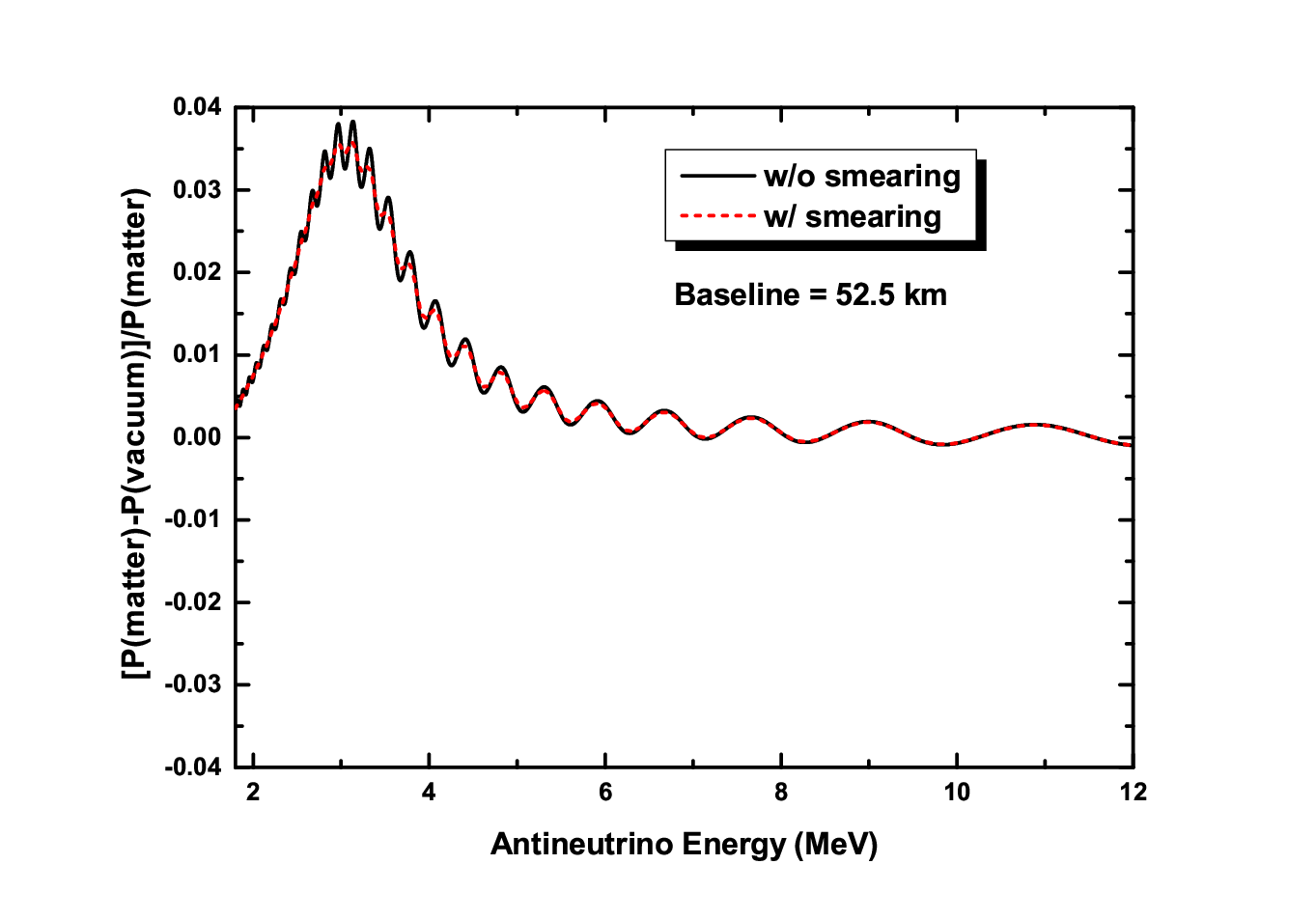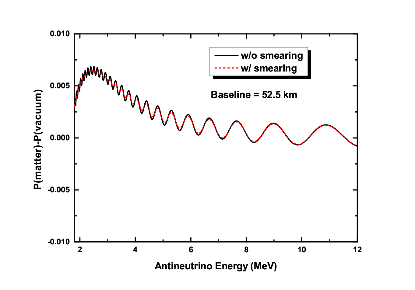
As a result of our exact numerical calculations without involving any analytical approximations, Fig. 1 shows the absolute (left panel) and relative (right panel) differences between the matter-corrected probability $\widetilde{P}(\overline{\nu}_{e}\to\overline{\nu}_{e})$ and its vacuum counterpart $P(\overline{\nu}_{e}\to\overline{\nu}_{e})$ associated with a medium-baseline ($L=52.5$ km) reactor antineutrino oscillation experiment. The solid curves are for the true antineutrino energy, and the dashed ones are averaged over a Gaussian energy resolution of 3%/$\sqrt{E\,(\rm MeV)}$. We see that the absolute difference $\widetilde{P}(\overline{\nu}_{e}\to\overline{\nu}_{e})-P(\overline{\nu}_{e}\to\overline{\nu}_{e})$ can reach about $0.7\%$ in the vicinity of the first oscillation peak of $\Delta_{21}$, which corresponds to a relative matter-induced correction of about $4\%$ illustrated on the right panel of Fig. 1. As a matter of fact, the main profile of $\widetilde{P}(\overline{\nu}_{e}\to\overline{\nu}_{e})-P(\overline{\nu}_{e}\to\overline{\nu}_{e})$ or $\left[\widetilde{P}(\overline{\nu}_{e}\to\overline{\nu}_{e})-P(\overline{\nu}_{e}\to\overline{\nu}_{e})\right]/\widetilde{P}(\overline{\nu}_{e}\to\overline{\nu}_{e})$ is attributed to the $\Delta_{21}$-triggered oscillation, where the matter-induced suppression in $\sin^{2}2\widetilde{\theta}_{12}$ provides a positive correction in the $\Delta_{21}$-dominated range. The small wiggles in Fig. 1 are caused by the $\Delta_{*}$-triggered oscillation, and their amplitudes are modulated by the energy-dependent correction of $\cos 2\widetilde{\theta}_{12}$.

Before calculating the statistical sensitivity of a realistic experimental measurement, it is necessary to test the accuracy of our analytical approximations made in Eqs. (8)—(11) and Eqs. (15)—(18). Fig. 2 shows a comparison between the results of $\widetilde{P}(\overline{\nu}_{e}\to\overline{\nu}_{e})$ obtained from a complete numerical calculation and the analytical approximations made in Eq. (18): their absolute (left panel) and relative (right panel) differences with or without smearing effects for a reactor antineutrino oscillation experiment like JUNO or RENO-50. In this figure the solid lines are for the true antineutrino energy, and the dashed curves are averaged over a Gaussian energy resolution of 3%/$\sqrt{E\,(\rm MeV)}$. We find that the absolute errors of our analytical approximations are lower than $3\times 10^{-4}$ in most of the antineutrino energy range, proving that Eq. (18) and the associated analytical approximations can be safely employed in the following sensitivity studies.

Taking account of JUNO’s nominal setup as described in Refs. [1, 20], we are going to illustrate how the terrestrial matter effects influence the measurements of both the neutrino mass ordering and the flavor mixing parameters. We shall also discuss an important issue: to what extent one can establish or constrain the terrestrial matter effects at JUNO or RENO-50, or in a similar experiment to be proposed.

Given the JUNO simulation, which has been described in detail in Ref. [1], let us consider a 20 kt liquid scintillator detector with the energy resolution of 3%/$\sqrt{E\,(\rm MeV)}$ ³³ 3 A generic parametrization of the energy resolution is written as $\sqrt{({a}/{\sqrt{E}})^{2}+b^{2}+({c}/{E})^{2}}$, which is numerically equivalent to an effective energy resolution of $\sqrt{{a}^{2}+(1.6\times b)^{2}+(c/1.6)^{2}}/{\sqrt{E}}$ in the mass ordering measurement [1]. The requirement of 3%/$\sqrt{E\,(\rm MeV)}$ can be regarded as the total contribution of all the stochastic and non-stochastic terms. . We take account of the real reactor powers and baseline distributions of the Yangjiang and Taishan nuclear power plants listed in Table 2 of Ref. [1], which have a total thermal power of 36 ${\rm GW}_{\rm th}$ and a power-weighted baseline of 52.5 km. Moreover, we assume a detection efficiency of 80% and the nominal running time of six years and 300 effective days per year in our numerical simulation.

To discuss the statistical sensitivity of the experimental measurement ⁴⁴ 4 See Refs. [1, 20, 21, 22, 23, 24, 25] for an incomplete list of the works dealing with the statistical sensitivity of the mass ordering measurement in a medium-baseline reactor antineutrino experiment., we construct the following standard $\chi^{2}$ function:

$$\chi^{2}=\sum^{N_{\text{bin}}}_{i=1}\frac{\left[M_{i}(p^{M},\eta)-T_{i}(p^{T},\eta)\left(1+\displaystyle\sum_{k}\alpha_{ik}\epsilon_{k}\right)\right]^{2}}{M_{i}(p^{M},\eta)}+\sum_{k}\frac{\epsilon^{2}_{k}}{\sigma^{2}_{k}}\,,$$

(20)

where $M_{i}$ and $T_{i}$ are the measured and predicted antineutrino events in the $i$-th antineutrino energy bin, respectively; $\sigma_{k}$ and $\epsilon_{k}$ are the $k$-th systematic uncertainty and the corresponding pull parameter, respectively. The considered nominal systematic uncertainties include the correlated reactor rate uncertainty ($\sim 2\%$), the uncorrelated reactor rate uncertainty ($\sim 0.8\%$), the energy-uncorrelated bin-to-bin reactor flux spectrum uncertainty ($\sim 1\%$) and the detector-related uncertainty ($\sim 1\%$). Some additional important systematic uncertainties on the measurements of the neutrino mass ordering and oscillation parameters have been thoroughly discussed in sections 2 and 3 of Ref. [1]. In Eq. (20), $p$ stands for the oscillation parameters (i.e., $p=\left\{\Delta_{21},\Delta_{*},\theta_{12},\theta_{13}\right\}$), and $\eta\equiv A(\rho)/A(\rho=2.6\;{\rm g/cm}^{3})$ is defined as the effective matter potential index.

Fig. 3 is a comparison of the neutrino mass ordering sensitivities with (solid) and without (dashed) considering the terrestrial matter effects. The black lines come from the fitting in the assumption of the normal mass ordering (NMO) of three neutrinos, and the red lines assume the inverted mass ordering (IMO). The vertical distance between the minima of the red and black curves is defined as a measure of the neutrino mass ordering sensitivity:

$$\Delta\chi^{2}_{\text{MO}}=\left|\chi^{2}_{\rm min}(\rm NMO)-\chi^{2}_{\rm min}(\rm IMO)\right|\;,$$

(21)

where the minimization is implemented for all the relevant oscillation and pull parameters. Compared with the situation of $\overline{\nu}_{e}\to\overline{\nu}_{e}$ oscillations in vacuum, the inclusion of terrestrial matter effects may reduce the value of $\Delta\chi^{2}_{\rm MO}$ from 10.28 to 9.64, which is comparable with other important systematic uncertainties and hence should not be neglected in the future mass ordering measurement. In the above calculation we have typically taken $\rho\simeq 2.6\;{\rm g/cm}^{3}$ for the terrestrial matter density. For the reactor antineutrino oscillations with a medium baseline (i.e., $L\sim 50$ km from the reactors to the detector), however, the $\overline{\nu}_{e}$ trajectory during propagation is expected to include a large proportion of the sedimentary layer. In other words, the realistic experiment may actually involve a somewhat smaller terrestrial matter density. In Fig. 4 we illustrate the sensitivity of the mass ordering measurement $\Delta\chi^{2}_{\rm MO}$ as a function of the matter potential index $\eta$. One can see that $\Delta\chi^{2}_{\rm MO}$ depends linearly on $\eta$. If a smaller matter density $\rho\simeq 2.0\;{\rm g/cm}^{3}$ is taken into account for JUNO, the mass ordering sensitivity reduction will be from 10.28 to 9.79.

Now we turn to discuss the terrestrial matter effects on the relevant flavor parameters. In our numerical analysis, $\rho\simeq 2.6\;{\rm g/cm}^{3}$ (i.e., $\eta\simeq 1$) is typically taken to modulate the measured antineutrino events $M_{i}$. In the left panel of Fig. 5 we include terrestrial matter effects in the predicted antineutrino events $T_{i}$ and display the fitting results of $\Delta_{21}$ and $\theta_{12}$. The red star denotes the true values of these two parameters. It turns out that the best-fit points can return to the true values, and the allowed regions are consistent with the fitting results in the assumption of the vacuum $\overline{\nu}_{e}\to\overline{\nu}_{e}$ oscillations (see section 3.2 of Ref. [1]). The 1$\sigma$ precision levels of $\Delta_{21}$ and $\sin^{2}\theta_{12}$ with the nominal systematic setup can reach $0.23\%$ and $0.58\%$, respectively. In comparison, the 1$\sigma$ precision levels of $\Delta_{21}$ and $\sin^{2}\theta_{12}$ in the absence of matter effects were found to be $0.24\%$ and $0.54\%$, respectively (see section 3.2 of Ref. [1]). A minor reduction in the accuracy of $\sin^{2}\theta_{12}$ is certainly attributed to the suppression of $\theta_{12}$ in terrestrial matter.

For the sake of comparison, let us neglect terrestrial matter effects in the predicted antineutrino events $T_{i}$ and illustrate the fitting results of $\Delta_{21}$ and $\theta_{12}$ in the right panel of Fig. 5. The red star points to the true values of these two parameters, and the blue dot stands for the best-fit point. The allowed regions are shifted to higher $\Delta_{21}$ and lower $\theta_{12}$, and the best-fit point is located at $\Delta_{21}\simeq 7.514\times 10^{-5}\;{\rm eV}^{2}$ and $\theta_{12}\simeq 33.26^{\circ}$. The precision of $\Delta_{21}$ and $\theta_{12}$ turns out to be the same as that in the left panel of Fig. 5. Hence the best-fit values of $\Delta_{21}$ and $\theta_{12}$ deviate around 0.8$\sigma$ and 2.4$\sigma$ from their true values, respectively. If additional systematic uncertainties [1] of the flux spectrum and the energy scale are taken into account in the analysis, the sizes of deviation might be more or less reduced.

Finally let us discuss to what extent one can establish or constrain the terrestrial matter effects at JUNO. Assuming a matter density $\rho\simeq 2.6\;{\rm g/cm}^{3}$ in the measured antineutrino events, we illustrate the change of $\Delta\chi^{2}(\eta)$ as a function of the matter potential index $\eta$ in Fig. 6 with both fixed and free oscillation parameters. If all the oscillation parameters are fixed, we obtain $\Delta\chi^{2}(0)\simeq 11$, indicating that the terrestrial matter effects can be tested with a significance of more than 3$\sigma$. However, the significance of establishing the terrestrial matter effects will significantly reduce to 1.3$\sigma$ after the oscillation parameters are marginalized. This can be understood with the help of Eqs. (11) and (17), where the corrections of the matter potential to $\sin^{2}\theta_{12}$ and $\Delta_{21}$ are about $0.8\%$ and $0.4\%$, respectively. If some additional systematic uncertainties are considered in the analysis [1], including the background, the reactor flux spectrum uncertainty of 1%, the energy scale uncertainty of 1% and the energy non-linear uncertainty of 1%, then the projected precision levels for $\sin^{2}\theta_{12}$ and $\Delta_{21}$ will be 0.72% and 0.60%, respectively. Correspondingly, the sensitivity of establishing the terrestrial matter effects will be less than 1$\sigma$.

If the near detectors can be built to monitor the reactor antineutrino flux, a relative measurement of the rate and spectrum between the near and far detectors is expected to significantly reduce the reactor- and detector-related systematic uncertainties in the $\sin^{2}\theta_{12}$ and $\Delta_{21}$ measurements, and thus the sensitivity of establishing the terrestrial matter effects can accordingly increase. Without specifying the details of near detectors, we just split the systematic uncertainties into the (detector-correlated) absolute uncertainties and (detector-uncorrelated) relative uncertainties. Assuming the absolute errors will be cancelled by virtue of near detectors and the relative errors are at the Daya Bay level [26, 27, 28, 29], we show the sensitivity of ruling out the vacuum neutrino oscillation scenario (i.e., $\eta=0$) as a function of the running time in Fig. 7, where the significance is defined as the squared root of ${\Delta\chi^{2}(\eta=0)}$. We observe that a 2$\sigma$ sensitivity of establishing the terrestrial matter effects can be achieved for about 10 years of data taking, if one or two appropriate near detectors are implemented to the nominal JUNO configuration. Further details on the near detector configuration will be discussed elsewhere ⁵⁵ 5 Given different motivation and different detector consideration, there are a few other works on the near detector ideas for a medium-baseline reactor antineutrino oscillation experiment [30, 31, 32]..

To summarize, we have examined how small the terrestrial matter effects can be in a medium-baseline reactor antineutrino oscillation experiment like JUNO or RENO-50, which aims to carry out a precision measurement of the neutrino mass ordering and relevant flavor parameters. To do so, we have expanded the probability of $\overline{\nu}_{e}\to\overline{\nu}_{e}$ oscillations with $L\simeq 50$ km in terms of the small matter parameter. Our analytical approximations are simple but accurate enough for a deeper understanding of the outputs of the exact numerical calculations. Taking the ongoing JUNO experiment as a good example, we have shown that the inclusion of terrestrial matter effects is likely to reduce the sensitivity of the neutrino mass ordering measurement by $\Delta\chi^{2}_{\rm MO}\simeq 0.6$. We find that the terrestrial matter effects may also shift the best-fit values of $\theta_{12}$ and $\Delta_{21}$ by about $1\sigma$ to $2\sigma$ if they are ignored in the future data analysis.

We conclude that the terrestrial matter effects must be carefully taken into account because they are non-negligible in the reactor-based measurements of the neutrino mass ordering and $\overline{\nu}_{e}\to\overline{\nu}_{e}$ oscillation parameters. But it remains difficult to establish the profile of terrestrial matter effects at a high significance level in a realistic experiment of this kind, such as JUNO or RENO-50. This issue motivates us to consider the possibility of installing the near detectors to measure the initial reactor antineutrino flux ⁶⁶ 6 We thank the useful communication with Jun Cao in this connection., where the matter effects have not been developed. In this case a comparison between the measurement of $\widetilde{P}(\overline{\nu}_{e}\to\overline{\nu}_{e})$ and its energy dependence at the far detector ($L\simeq 50$ km) and that of $P(\overline{\nu}_{e}\to\overline{\nu}_{e})$ at the near detectors ($L\sim 0$) will allow one to probe the fine effects of terrestrial matter associated with JUNO or RENO-50. Our preliminary estimate indicates that it is possible to establish the terrestrial matter effects with a $2\sigma$ sensitivity for about 10 years of data taking at JUNO with the help of a proper near detector implementation.

We thank Eligio Lisi, Shun Zhou and Jing-yu Zhu for useful discussions. This work was supported in part by the National Natural Science Foundation of China under Grant Nos. 11135009 and 11305193, by the Strategic Priority Research Program of the Chinese Academy of Sciences under Grant No. XDA10010100, and by the CAS Center for Excellence in Particle Physics.

References

- [1] F. An et al. [JUNO Collaboration], Neutrino Physics with JUNO, J. Phys. G 43 (2016) 030401 [arXiv:1507.05613 [physics.ins-det]].
- [2] Z. Djurcic et al. [JUNO Collaboration], JUNO Conceptual Design Report, (2015) arXiv:1508.07166 [physics.ins-det].
- [3] X. Qian and P. Vogel, Neutrino Mass Hierarchy, Prog. Part. Nucl. Phys. 83 (2015) 1 [arXiv:1505.01891 [hep-ex]].
- [4] R. B. Patterson, Prospects for Measurement of the Neutrino Mass Hierarchy, Ann. Rev. Nucl. Part. Sci. 65 (2015) 177 [arXiv:1506.07917 [hep-ex]].
- [5] S. B. Kim, New results from RENO and prospects with RENO-50, Nucl. Part. Phys. Proc. 265–266 (2015) 93 [arXiv:1412.2199 [hep-ex]].
- [6] F. Capozzi, E. Lisi and A. Marrone, Neutrino mass hierarchy and electron neutrino oscillation parameters with one hundred thousand reactor events, Phys. Rev. D 89 (2014) 013001 [arXiv:1309.1638 [hep-ph]].
- [7] Y. F. Li and Y. L. Zhou, Shifts of neutrino oscillation parameters in reactor antineutrino experiments with non-standard interactions, Nucl. Phys. B 888 (2014) 137 [arXiv:1408.6301 [hep-ph]]; and Y. F. Li, in section 3.2 of Ref. [1].
- [8] F. Capozzi, E. Lisi and A. Marrone, Neutrino mass hierarchy and precision physics with medium-baseline reactors: Impact of energy-scale and flux-shape uncertainties, Phys. Rev. D 92 (2015) 093011 [arXiv:1508.01392 [hep-ph]].
- [9] L. Wolfenstein, Neutrino oscillations in matter, Phys. Rev. D 17 (1978) 2369.
- [10] S. P. Mikheev and A. Y. Smirnov, Resonance amplification of oscillations in matter and spectroscopy of solar neutrinos, Sov. J. Nucl. Phys. 42 (1985) 913 [Yad. Fiz. 42 (1985) 1441].
- [11] H. Zhang and Z. z. Xing, Leptonic unitarity triangles in matter, Eur. Phys. J. C 41 (2005) 143 [hep-ph/0411183].
- [12] Z. z. Xing and J. y. Zhu, Matter-enhanced CP violation and Dirac unitarity triangles in a low-energy medium-baseline neutrino oscillation experiment, arXiv:1603.02002 [hep-ph].
- [13] See, e.g., I. Mocioiu and R. Shrock, Matter effects on neutrino oscillations in long baseline experiments, Phys. Rev. D 62 (2000) 053017 [hep-ph/0002149].
- [14] K. A. Olive et al. [Particle Data Group Collaboration], Review of particle physics, Chin. Phys. C 38 (2014) 090001.
- [15] F. Capozzi, G. L. Fogli, E. Lisi, A. Marrone, D. Montanino and A. Palazzo, Status of three-neutrino oscillation parameters, circa 2013, Phys. Rev. D 89 (2014) 093018 [arXiv:1312.2878 [hep-ph]].
- [16] F. Capozzi, E. Lisi, A. Marrone, D. Montanino and A. Palazzo, Neutrino masses and mixings: Status of known and unknown parameters, arXiv:1601.07777 [hep-ph].
- [17] D. V. Forero, M. Tortola and J. W. F. Valle, Neutrino oscillations refitted, Phys. Rev. D 90 (2014) 9, 093006 [arXiv:1405.7540 [hep-ph]].
- [18] M. C. Gonzalez-Garcia, M. Maltoni and T. Schwetz, Updated fit to three neutrino mixing: status of leptonic CP violation, JHEP 1411 (2014) 052 [arXiv:1409.5439 [hep-ph]].
- [19] Y. Wang and Z. z. Xing, Neutrino Masses and Flavor Oscillations, arXiv:1504.06155 [hep-ph].
- [20] Y. F. Li, J. Cao, Y. Wang and L. Zhan, Unambiguous Determination of the Neutrino Mass Hierarchy Using Reactor Neutrinos, Phys. Rev. D 88 (2013) 013008 [arXiv:1303.6733 [hep-ex]].
- [21] X. Qian, D. A. Dwyer, R. D. McKeown, P. Vogel, W. Wang and C. Zhang, Mass Hierarchy Resolution in Reactor Anti-neutrino Experiments: Parameter Degeneracies and Detector Energy Response, Phys. Rev. D 87 (2013) 033005 [arXiv:1208.1551 [physics.ins-det]].
- [22] S. F. Ge, K. Hagiwara, N. Okamura and Y. Takaesu, Determination of mass hierarchy with medium baseline reactor neutrino experiments, JHEP 1305 (2013) 131 [arXiv:1210.8141 [hep-ph]].
- [23] E. Ciuffoli, J. Evslin and X. Zhang, Neutrino mass hierarchy from nuclear reactor experiments, Phys. Rev. D 88 (2013) 033017 [arXiv:1302.0624 [hep-ph]].
- [24] M. Blennow, P. Coloma, P. Huber and T. Schwetz, Quantifying the sensitivity of oscillation experiments to the neutrino mass ordering, JHEP 1403 (2014) 028 [arXiv:1311.1822 [hep-ph]].
- [25] M. Y. Pac, Experimental Conditions for Determination of the Neutrino Mass Hierarchy with Reactor Antineutrinos, Nucl. Phys. B 902 (2016) 326 [arXiv:1508.01650 [hep-ex]].
- [26] F. P. An et al. [Daya Bay Collaboration], Observation of electron-antineutrino disappearance at Daya Bay, Phys. Rev. Lett. 108 (2012) 171803 [arXiv:1203.1669 [hep-ex]].
- [27] F. P. An et al. [Daya Bay Collaboration], Improved Measurement of Electron Antineutrino Disappearance at Daya Bay, Chin. Phys. C 37 (2013) 011001 [arXiv:1210.6327 [hep-ex]].
- [28] F. P. An et al. [Daya Bay Collaboration], Spectral measurement of electron antineutrino oscillation amplitude and frequency at Daya Bay, Phys. Rev. Lett. 112 (2014) 061801 [arXiv:1310.6732 [hep-ex]].
- [29] F. P. An et al. [Daya Bay Collaboration], New Measurement of Antineutrino Oscillation with the Full Detector Configuration at Daya Bay, Phys. Rev. Lett. 115 (2015) 111802 [arXiv:1505.03456 [hep-ex]].
- [30] A. B. Balantekin et al., Neutrino mass hierarchy determination and other physics potential of medium-baseline reactor neutrino oscillation experiments, arXiv:1307.7419 [hep-ex].
- [31] E. Ciuffoli, J. Evslin, Z. Wang, C. Yang, X. Zhang and W. Zhong, Advantages of Multiple Detectors for the Neutrino Mass Hierarchy Determination at Reactor Experiments, Phys. Rev. D 89 (2014) 073006 [arXiv:1308.0591 [hep-ph]].
- [32] H. Wang, L. Zhan, Y. F. Li, G. Cao and S. Chen, Mass hierarchy sensitivity of medium baseline reactor neutrino experiments with multiple detectors, arXiv:1602.04442 [physics.ins-det].
Abstract
We have carefully examined, in both analytical and numerical ways, how small the terrestrial matter effects can be in a given medium-baseline reactor antineutrino oscillation experiment like JUNO or RENO-50. Taking the ongoing JUNO experiment for example, we show that the inclusion of terrestrial matter effects may reduce the sensitivity of the neutrino mass ordering measurement by , and a neglect of such effects may shift the best-fit values of the flavor mixing angle and the neutrino mass-squared difference by about to in the future data analysis. In addition, a preliminary estimate indicates that a sensitivity of establishing the terrestrial matter effects can be achieved for about 10 years of data taking at JUNO with the help of a proper near detector implementation.