Born-Infeld cosmology with scalar Born-Infeld matter
Abstract
Cosmology in Eddington-inspired Born-Infeld gravity is investigated using a scalar Born-Infeld field (e.g. tachyon condensate) as matter. In this way, both in the gravity and matter sectors we have Born-Infeld-like structures characterized by their actions and via two separate constants, and respectively. With a particular choice of the form of (the time derivative of the Born-Infeld scalar), analytical cosmological solutions are found. Thereafter, we explore some of the unique features of the corresponding cosmological spacetimes. For , our solution has a de Sitter-like expansion both at early and late times, with an intermediate deceleration sandwiched between the accelerating phases. On the other hand, when , the initial de Sitter phase is replaced by a bounce. Our solutions, at late time, fit well with available supernova data– a fact we demonstrate explicitly. The estimated properties of the Universe obtained from the fitting of the solution, are as good as in CDM cosmology. However, the solution has to be discarded due to the occurrence of a bounce at an unacceptably low redshift.
pacs
04.20.-q, 04.20.JbI Introduction
General relativity (GR) is largely successful as a classical theory of gravity, especially with the recent detection of gravitational waves. However, there do exist many unsolved puzzles. Among them is the problem of singularities in GR which is expected to be resolved by quantum gravity. Dark matter and dark energy also do not seem to be well understood within the framework of GR. Thus, in order to address some of the above-mentioned problems, it is not unusual to construct theories which deviate from GR within the classical framework, inside matter distributions, or in the strong-field regime. This expectation has led many researchers to actively pursue modified theories of gravity in the classical domain and also in quantum theory. One such modification is inspired by the well-known Born-Infeld electrodynamics where we are able to regularize the infinity in the electric field at the location of a point charge [1]. With a similar determinantal structure as in the action of Born-Infeld electrodynamics, a gravity theory in the metric formulation was first suggested by Deser and Gibbons [2]. In fact, the determinantal form of the gravitational action existed earlier in Eddington’s re-formulation of GR in de Sitter spacetime [3]. This formulation is affine and the connection is the basic variable instead of the metric. However, the coupling of matter remained a problem in Eddington’s approach.
Later, Vollick [4] introduced the Palatini formulation of Born-Infeld gravity and worked on various related aspects. He also introduced a nontrivial and somewhat artificial way of coupling matter in such a theory [5, 6]. More recently, Banados and Ferreira [7] have come up with a formulation where the matter coupling is different and simpler compared to Vollick’s proposal. We will focus here on the theory proposed in Ref. [7] and refer to it as Eddington-inspired Born–Infeld (EiBI) gravity, for obvious reasons. Note that the EiBI theory has the feature that it reduces to GR in vacuum.
Interestingly, EiBI theory also falls within the class of bimetric theories of gravity (also called bi-gravity). The current bimetric theories have their origin in the seminal work of Isham, Salam and Strathdee [8]. Several articles have appeared in the last few years on various aspects of such bi-gravity theories. In Ref. [9], the authors pointed out that the EiBI field equations can also be derived from an equivalent bi-gravity action. This action is closely related to a recently discovered family of unitary massive gravity theories which are built as bi-gravity theories. Several others have contributed in this direction, in various ways [10, 11].
Let us now briefly recall Eddington–inspired Born–Infeld gravity. The central feature here is the existence of a physical metric which couples to matter and another auxiliary metric which is not used for matter couplings. One needs to solve for both metrics through the field equations. The action for the theory developed in Ref. [7] is given as
| (1) |
where . Variation with respect to , done using the auxiliary metric , gives
| (2) |
Variation with respect to gives
| (3) |
where the components are in the coordinate frame. In order to obtain solutions, we need to assume a and a with unknown functions, as well as a matter stress-energy (). Thereafter, we write down the field equations and obtain solutions using some additional assumptions about the metric functions and the stress-energy.
Work on various fronts has been carried out on various aspects of this theory in the last few years. Astrophysical scenarios have been discussed in Refs. [12, 13, 14, 15, 16, 17, 18, 19, 20]. Spherically symmetric solutions were obtained in Refs. [7, 21, 22, 23, 24, 25]. A domain wall brane in a higher-dimensional generalization was analyzed in Ref. [26]. Generic features of the paradigm of matter-gravity couplings were analyzed in Ref. [27]. In Ref. [28], authors showed that EiBI theory admits a nongravitating matter distribution, which is not allowed in GR. Some interesting cosmological and circularly symmetric solutions in dimensions were shown in Ref. [29]. Constraints on the EiBI parameter have been obtained from studies on compact stars [12, 16], tests in the Solar System [30], astrophysical and cosmological observations [14], and nuclear physics studies [31]. In Ref. [32], a major problem related to surface singularities was noticed in the context of stellar physics. However, gravitational backreaction was suggested as a cure to this problem in Ref. [33]. In Ref. [34], the authors proposed a modification to EiBI theory by taking its functional extension in a way similar to theory. Recently, the authors of Ref. [35] used a different way of matter coupling by taking the Kaluza ansatz for the five-dimensional EiBI action in a purely metric formulation, and then compactify it using Kaluza’s procedure to get a four-dimensional gravity coupled in a nonlinear way to electromagnetic theory.
Much work in EiBI gravity is devoted to cosmology. In Refs. [7, 9, 36], the authors showed the nonsingularity of the Universe filled by any ordinary matter. Linear perturbations have been studied in the background of the homogeneous and isotropic spacetimes in the Eddington regime [37, 38]. Bouncing cosmology in EiBI gravity was emphasized as an alternative to inflation in Ref. [39]. The authors of Ref. [40] studied a model described by a scalar field with a quadratic potential, which results in a nonsingular initial state of the Universe leading naturally to inflation. They also investigated the stability of the tensor perturbations in this inflationary model [41] while the scalar perturbation was studied in Ref. [42]. Other relevant work has been reported in Refs. [43, 44, 45]. Large-scale structure formation in the Universe and the integrated Sachs-Wolfe effect are discussed in Ref. [46]. Further efforts in this line were reported in Refs. [47, 48, 49, 50].
In Ref. [25], we considered the Born-Infeld structure in both the gravity and matter sectors and obtained new spherically symmetric static spacetimes when EiBI gravity is coupled to Born-Infeld electrodynamics. In this article, we investigate a similar problem in EiBI cosmology where we consider a Born-Infeld scalar field in the matter part. In particular, we use the tachyon condensate scalar because of its Born-Infeld-like structure in the action. The tachyon condensate scalar field arises in the context of theories of unification such as superstring theory [51]. There have been several articles in the literature where cosmology with the tachyon scalar field was discussed [52, 53, 54, 55, 56, 57, 58, 59, 60, 61, 62, 63, 64]. The energy-momentum tensor of the BI scalar tachyon condensate can be split into two parts; one with zero pressure (dark matter) and another with (dark energy) [65]. This facilitates the description of dark energy and dark matter using a single scalar field, a fact we shall use for our model in this article.
We organize our article as follows. In Sec. II we discuss the basic setup of the BI scalar field in the cosmological background. Next, in Sec. III we obtain a constant negative (effective) pressure solution as the special case of the general assumption on the form of the time derivative of the scalar field. Then, we fit the solutions with the supernova data and test its viability in Sec. IV. Finally, in Sec. V we summarize our results.
II Cosmology with a Born-Infeld scalar
The action for the BI scalar (eg. tachyon condensate)is
| (4) |
where, is the potential for the scalar field and is the constant parameter. The resulting stress-energy tensor components have the following general expression:
| (5) | |||||
By varying the action with respect to (w.r.t.) , we get the equation of motion of the scalar field
| (6) |
where is derivative of the potential w.r.t. the scalar field. The equation (6) also ensures the conservation of the stress-energy tensor (). For a homogeneous and isotropic, spatially flat Universe, we assume the following ansatz for the physical spacetime metric:
| (7) |
The equation (6) leads to the following equation of motion of the scalar field ():
| (8) |
where dots denote the derivatives w.r.t. and primes denote the derivatives w.r.t. . Also, the stress-energy tensor for the BI scalar field can be re-written as that of an analogous perfect fluid, , where and are the equivalent pressure and energy density, respectively, in the comoving frame. The and are expressed in terms of the scalar field as
| (9) | |||||
| (10) |
We can re-express the scalar potential in terms of and in the following way,
| (11) |
Using Eqs. (9) and (10), Eq. (8) can be rewritten as
| (12) |
Generally, in a scalar field cosmology, we choose the form of the potential for the scalar field. This is because we do have an extra degree of freedom in the field equations. Here, we exploit this and choose the form of instead of . We assume the form of as
| (13) |
where and . Thus, using the Eq. (13) we solve Eq. (12) and obtain
| (14) | |||||
| (15) |
where is an integration constant. At this point, is just a scaling parameter for the scalar field and the potential. But this is changed if we relate with . We choose . Then the potential becomes [from Eq. (11)]
| (16) |
where the potential is now expressed in terms of the scale factor in parametrized form. For this choice of , for . This becomes a universal character ( for arbitrary ). For , and . On the other hand, for the given and , becomes the control parameter for modifying the behaviour of the potential and all other quantities in the early Universe.
III A constant negative pressure solution
In GR, the cosmological solution with a constant negative pressure can be found. It may be a bouncing solution where the scale factor is given by
| (17) |
The corresponding energy density profile is
| (18) |
The other possibility is of a singular solution where the scale factor and the energy density are given by
| (19) | |||
| (20) |
In EiBI gravity coupled to a BI scalar, with the choice of in Eq. (15), (constant negative pressure). We would now like to construct the solution for the physical line element. Let us assume an ansatz for the auxiliary metric
| (21) |
From the Eq. (3) we get two independent equations which we rewrite in the following way,
| (22) | |||||
| (23) |
where is a new constant parameter. Note that has both and in its definition. We will see that is one of the parameters which we will use while fitting our final solution with supernova observations. We also assume (). From the variation, we further have two independent equations [Eq. (2)]. After a simple algebraic manipulation these two equations become
| (24) | |||
| (25) |
To obtain the solution, we need to solve the four equations (22), (23), (24), and (25). However, we have five unknowns: and . Therefore, we have the freedom to choose the functional form of any one of the unknowns. Since we are free to choose the auxiliary metric functions we assume , where and are two arbitrary nonzero constants. Thus, from Eq. (24), we arrive at
| (26) |
The above quadratic equation (26) has two roots. We choose the one for which . Therefore, we have
| (27) |
Further, from Eq. (25), we have
| (28) |
At this juncture, we introduce a new variable and rewrite the Eq. (28) as
| (29) |
Integrating the Eq. (29), we get
| (30) |
where is the constant of integration. Using Eqs. (22), (26), and (30), we compare the two expressions of –one from field equations ( Eq. 23) and the other from the conservation equation ( Eq. 14). Since the field equations in EiBI theory satisfy the conservation equation, the constant is fixed and has the expression: . The new variable is related to . Since appears in the auxiliary metric as a coefficient of , is, in a sense related to a redefinition of the time variable. In what follows, we will see this connection more explicitly.
III.1
Using Eqs. (22), (27), and (30) we rewrite the expression of as a function of :
| (31) |
From Eq. (14), we note that for and . So, necessitates . Then, for , and maps onto . Similarly, we express the other metric function and the coordinate as functions of
| (32) | |||||
| (33) |
where is an arbitrary constant. The relation between and in Eq. (33) is invertible and we may write as a function of though the expression takes a complicated form. Therefore, it is better to express the metric functions and of the physical metric [Eq. (7)] in parametric form [Eqs. (31), (32), and (33)], where is the parameter. We define the cosmological time
| (34) | |||||
In order to understand the evolution of , we compute the deceleration parameter ()
| (35) | |||||
Interestingly, we note that, for ( ), . Also, for ( ), . Therefore, both at early and late times, the Universe undergoes a de Sitter phase in our model. Also, for some values of , the Universe may undergo a decelerated expansion state () [see Fig. 1].

Using Eqs. (31) and (34), we plot the scale factor as a function of the cosmological time () [Fig:2]. In the plot, we choose a value of such that we are able to note an initial loitering phase (with an acceleration) followed by a decelerated expansion phase and then an accelerated expansion at late times. From Fig. 2, we note that the effective energy density () decreases as increases and approaches a nonzero minimum value at large . Though diverges at , it takes an infinite time () to reach that point. Thus, the Universe is nonsingular. Such a nonsingular de Sitter inflationary phase is a common feature of the Universe with constant pressure, in EiBI cosmology. The accelerated expansion of the Universe at late times is due to the fact that at late times the effective pressure () is related to the energy density () as . The decelerated expansion in between the two accelerated phases is due to the fact that the repulsive nature of gravitating matter is less dominant than its attractive character, during this phase.


In Fig. 3, we show the variation of the scalar field as a function of , which results in such a cosmological solution. We also plot the associated potential as a function of . An analytical expression for as a function of is, unfortunately, not available due to the non-invertible nature of . We use Eqs. (13), (16), and (34) for the plotting. Here, the scalar field could be either decaying or growing in time for the same solution [see Eq. (13)]. These features are shown in the top and bottom panels respectively, with the associated potentials. However, in both situations, the potentials approach a nonzero minimum value and that occurs at late times of the Universe.


During the loitering phase, the scale factor grows exponentially (). On the other hand, it can be shown that during the period of inflation, the Universe expanded by a factor of in seconds. Using this as input, the bound on becomes which is greater than the Planck length square (). However, the de Sitter expansion of the Universe at very late times is different from it and depends on the other BI parameter (). Thus, in two different extreme regimes, the evolution of the scale factor depends on the two BI parameters independently. However, the intermediate phase depends on the product of these two parameters ().
III.2
For , implies that [see Eq. (31)]. For , , but for , . Also, we note that at . So, for , there is a nonzero minimum scale factor at which the Universe undergoes a bounce. In Fig. 4, the deceleration parameter () is plotted as a function for different values of . Since , so ; we also assume . In Fig. 4, we note that as (near the bounce). This is because at , , but has a nonzero finite value. However, in this case too, the Universe undergoes a de Sitter stage at late times ( for ).
In Fig. 5, we show the variation of the scale factor ( ) as a function of the cosmological time (). We choose the parameter values in such a way that we see the bounce followed by decelerated expansion and finally the de Sitter stage at late times. The plot of the effective energy density () in the Fig. 5 shows a regular profile throughout. Here we mention that the nonsingular bouncing early Universe is a common feature of EiBI cosmology. The BI scalar field provides the additional late time acceleration.
In Fig. 6, we plot the scalar field () and the associated potential . We note that, for both decaying and growing nature of the scalar field, the potential remains invariant.


IV Observational test of the solutions from fitting the supernova data
So far we have found that the resulting cosmological solutions exhibit an early-time accelerated expansion as well as a late-time acceleration. There can also exist a phase of decelerated expansion lying in between the two acclerated phases. For , the early Universe grows exponentially (similar to an inflationary scenerio) and for , the early Universe undergoes a bounce. In this section, we fit the aforementioned solutions with the supernova data and test their viability in describing the evolution of the Universe at late times. However, we do not consider any other field as a part of the matter sector apart from the BI scalar field. Here, we follow the approach adopted in [65], where the BI scalar field is treated as a single candidate having the capacity of exhibiting different equations of state at different scales and making a transition from (cold dark matter) at small scales to (dark energy) at large scales. The total energy density is, likewise, split into two parts: pressureless dust and dark energy,
| (36) |
Thus, from Eqs. (9) and (10), we get
| (37) |
In our case, we get and (a constant) [see Eqs. (14) and (15) with and ]. This is similar to CDM cosmology. However, the cosmological constant is not an ad-hoc quantity but generated from the BI scalar field with a specific choice of (or, alternatively with an equivalent choice of the potential function).
IV.1
Using Eqs. (31) and (34), we rewrite the Hubble function as
| (38) |
where is the redshift defined as . and are the present day values of the Hubble function and . The expressions for and are given as
| (39) | |||||
| (40) |
where, . Using the Eqs. (38) and (39), we can define the luminosity distance for the observed supernova at the redshift as , where is the Hubble free luminosity distance. Therefore, the Hubble free luminosity distance becomes
| (41) | |||||
Using Eq. (41) as the model, we fit the supernova data. There are two parameters and , which are both dimensionless. From the best fit parameter values (of and ), we can estimate the best fit values of (present day value of the deceleration parameter), (ratio of present day matter density to total energy density of the Universe), (for dark energy), , and .To carry out all of this, we write down the useful relations next. We use Eq. (35) to evaluate . We get the expression of in terms of and , [using Eqs. (23), (31), and (40)]
| (42) |
Further, can also be expressed as
| (43) |
where and . We can evaluate using
| (44) |
Finally, the expression of is
| (45) |
where, we use a prior value of .
To fit the Supernova data with our model, we follow the method used in [66], wherein the authors have studied the expansion history of the universe upto a redshift using the 194 Type Ia supernovae (SNe Ia) data. However, in our case we use the more recent Union2.1 Compilation data [67]. The observational dataset consists of the values of the distance modulus () and redshifts with their corresponding errors. Each distance modulus is related to the corresponding luminosity distance of the SNe Ia by
| (46) |
The observed distance modulus can be translated to . For a given model , one can also theoretically predict the using the Eq. (41). The best fit values of the model parameters () are estimated by minimizing the which, in this case, is given by [66]
| (47) |
where is redshift uncertainty of the data and is the error of . The error in redshift is estimated from the uncertainty due to peculiar velocities, , i.e. .
The resulting best fit parameter values are
| (48) |
If (: number of data points, : number of parameters), the fit is good and the data are consistent with the considered model . Here, . In Fig. 7, the variation of the luminosity distance with respect to the redshift is shown for the best fit parameter values, along with the observed data points. In Fig. 7, we show the and confidence levels in the parameter space .

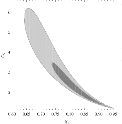
Using the best fit parameter values, the estimated values of , , and are
| (49) |
These are in reasonably good agreement with CDM cosmology [67]. Further, we plot and in Fig. 8. This figure once again demonstrates the viability of our model with observations, at least at late times.
We mention an important point here. Using the critical energy density of the Universe as obtained in the framework of GR (i.e. ), one can write down the present-day values of the density parameters corresponding to dark matter and dark energy as and . Here, , as it should be in a modified theory of gravity. In our case, with the best fit values of the parameters and , we find that is very close (but not equal) to one ( and ). Therefore, irrespective of our definition of the density parameters, our model for late-time evolution seems to work well.

The estimated value of the theory parameter for the EiBI gravity and the value of the parameter for the scalar field (matter) sector are
| (50) |
Using , , and , we can define mass (), time (), and length (). , , and .
IV.2
We also fit the bouncing () solution with the same supernovae data. In this case, the expression for the luminosity distance function becomes
| (51) | |||||
| (52) | |||||
| (53) | |||||
| (54) |
Here, and . The minimum scale factor () corresponds to the maximum redshift . The best fit parameter values are , with . Using the best fit value of in Eq. (53), the maximum redshift becomes . This is absurd as should be greater than the redshift corresponding to CMB radiation (). Thus the bouncing Universe model is ruled out though it fits well with the data.
V Conclusions
Let us now briefly summarize our findings.
We have looked at cosmologies in EiBI gravity with a Born-Infeld scalar (tachyon condensate) in the matter part of the total action. Thus, we have incorporated a Born-Infeld structure in both the gravity and the matter sectors of the theory. We have two control parameters; of dimension for the gravity sector and the dimensionless for the matter sector.
In our approach here, we have assumed a form of instead of assuming a scalar potential. For a particular choice of a parameter (i.e. ), the problem reduces to a situation where the Universe is driven by a perfect fluid of constant negative pressure. We obtain the analytical solution for such a set up. For , the Universe undergoes a de Sitter expansion stage both at early and late times. In between, there could be a decelerated expansion depending on the value of . For , there is a difference in the picture through the occurrence of a bounce instead of the de Sitter expansion at early times. However, at late times, the Universe still undergoes the de Sitter expansion even for .
Qualitatively, similar behaviour can also be achieved for in the form of (Eq. 13). For such a different choice, the effective pressure becomes bounded. This is named the Maximal Pressure State (MPS) in [40], which provides a de Sitter stage in the expansion history of the Universe at the early times for , in EiBI gravity. But for and , a similar bounce does occur supporting the generic bounce character in EiBI cosmology. We also note that, in our case, the equation of a state for the BI scalar (tachyon condensate) becomes at late times. Thus, at late times, the Universe undergoes a de Sitter expansion phase. In fact, it seems that we do not need any exotic matter source for producing late time acceleration in EiBI gravity, due to the above-mentioned property.
We have split the total energy-momentum tensor of the BI scalar (tachyon condensate) into two parts: one for dark matter () and the other as dark energy (). In our special case ( in the equation of ), the dark energy has constant negative pressure. Therefore, this is equivalent to CDM cosmology though the effective cosmological constant is generated from the BI scalar. However, for , we would have an evolving dark energy.
It may be noted that though we have a viable background cosmological model, issues such as inflation and reheating will have to be addressed in greater detail. We hope future investigations will throw light on these topics.
We have shown that the supernova data fit well with both the late time solutions for and . However, we discard the solution because our fit predicts an unacceptable value of the redshift where the Universe may undergo a bounce. With a different choice of and additional matter, it may be possible to introduce new parameters and obtain a viable solution. Remarkably, the cosmological properties estimated from the supernova data fit of the solution is as good as in CDM cosmology. It is possible that instead of using the special case , one may use the general form of and keep as an additional fitting parameter, in order to figure out how dark energy evolves.
Since we have analytical solutions which are not too complicated, it may be worthwhile to attempt a study of cosmological perturbations using this model as a background cosmology. Such a study with adequate observational tests and checks will surely help in establishing EiBI cosmology on a firmer footing, in future.
References
- [1] M. Born and L. Infeld, Proc. R. Soc. A 144, 425 (1934)
- [2] S. Deser and G. W. Gibbons, Classical and Quantum Gravity 15, L35 (1998)
- [3] A. Eddington, The Mathematical Theory of Relativity (Cambridge University Press, Cambridge, England, 1924)
- [4] D. N. Vollick, Phys. Rev. D 69, 064030 (2004)
- [5] D. N. Vollick, Phys. Rev. D 72, 084026 (2005)
- [6] D. N. Vollick, arXiv:gr-qc/0601136
- [7] M. Bañados and P. G. Ferreira, Phys. Rev. Lett. 105, 011101 (2010)
- [8] C. J. Isham, A. Salam, and J. Strathdee, Phys. Rev. D 3, 867 (1971)
- [9] J. H. C. Scargill, M. Banados, and P. G. Ferreira, Phys. Rev. D 86, 103533 (2012)
- [10] A. Schmidt-May and M. von Strauss(2014), arXiv:1412.3812 [hep-th]
- [11] J. B. Jiménez, L. Heisenberg, and G. J. Olmo, Journal of Cosmology and Astroparticle Physics 2014, 004 (2014)
- [12] P. Pani, V. Cardoso, and T. Delsate, Phys. Rev. Lett. 107, 031101 (2011)
- [13] J. Casanellas, P. Pani, I. Lopes, and V. Cardoso, The Astrophysical Journal 745, 15 (2012)
- [14] P. P. Avelino, Phys. Rev. D 85, 104053 (2012)
- [15] Y.-H. Sham, L.-M. Lin, and P. T. Leung, Phys. Rev. D 86, 064015 (2012)
- [16] Y.-H. Sham, P. T. Leung, and L.-M. Lin, Phys. Rev. D 87, 061503 (2013)
- [17] T. Harko, F. S. N. Lobo, M. K. Mak, and S. V. Sushkov, Phys. Rev. D 88, 044032 (2013)
- [18] H. Sotani, Phys. Rev. D 89, 104005 (2014)
- [19] H. Sotani, Phys. Rev. D 89, 124037 (2014)
- [20] H. Sotani(2015), arXiv:1503.07942 [astro-ph.HE]
- [21] S.-W. Wei, K. Yang, and Y.-X. Liu(2014), arXiv:1405.2178 [gr-qc]
- [22] H. Sotani and U. Miyamoto, Phys. Rev. D 90, 124087 (2014)
- [23] G. J. Olmo, D. Rubiera-Garcia, and H. Sanchis-Alepuz, The European Physical Journal C 74, 2804 (2014)
- [24] R. Shaikh, Phys. Rev. D 92, 024015 (2015)
- [25] S. Jana and S. Kar, Phys. Rev. D 92, 084004 (2015)
- [26] Y.-X. Liu, K. Yang, H. Guo, and Y. Zhong, Phys. Rev. D 85, 124053 (2012)
- [27] T. Delsate and J. Steinhoff, Phys. Rev. Lett. 109, 021101 (2012)
- [28] I. Cho and H.-C. Kim, Phys. Rev. D 88, 064038 (2013)
- [29] S. Jana and S. Kar, Phys. Rev. D 88, 024013 (2013)
- [30] J. Casanellas, P. Pani, I. Lopes, and V. Cardoso, The Astrophysical Journal 745, 15 (2012)
- [31] P. Avelino, Journal of Cosmology and Astroparticle Physics 2012, 022 (2012)
- [32] P. Pani and T. P. Sotiriou, Phys. Rev. Lett. 109, 251102 (2012)
- [33] H.-C. Kim, Phys. Rev. D 89, 064001 (2014)
- [34] S. D. Odintsov, G. J. Olmo, and D. Rubiera-Garcia, Phys. Rev. D 90, 044003 (2014)
- [35] K. Fernandes and A. Lahiri, Phys. Rev. D 91, 044014 (2015)
- [36] I. Cho, H.-C. Kim, and T. Moon, Phys. Rev. D 86, 084018 (2012)
- [37] C. Escamilla-Rivera, M. Banados, and P. G. Ferreira, Phys. Rev. D 85, 087302 (2012)
- [38] K. Yang, X.-L. Du, and Y.-X. Liu, Phys. Rev. D 88, 124037 (2013)
- [39] P. P. Avelino and R. Z. Ferreira, Phys. Rev. D 86, 041501 (2012)
- [40] I. Cho, H.-C. Kim, and T. Moon, Phys. Rev. Lett. 111, 071301 (2013)
- [41] I. Cho and H.-C. Kim, Phys. Rev. D 90, 024063 (Jul 2014), http://link.aps.org/doi/10.1103/PhysRevD.90.024063
- [42] I. Cho and N. K. Singh, European Physical Journal C 75, 240 (Jun. 2015), arXiv:1412.6344 [gr-qc]
- [43] I. Cho and J.-O. Gong, Phys. Rev. D 92, 064046 (2015)
- [44] I. Cho and N. K. Singh, Phys. Rev. D 92, 024038 (2015)
- [45] I. Cho and N. K. Singh, European Physical Journal C 74, 3155 (Nov. 2014), arXiv:1408.2652 [gr-qc]
- [46] X.-L. Du, K. Yang, X.-H. Meng, and Y.-X. Liu, Phys. Rev. D 90, 044054 (2014)
- [47] A. De Felice, B. Gumjudpai, and S. Jhingan, Phys. Rev. D 86, 043525 (2012)
- [48] M. Lagos, M. Bañados, P. G. Ferreira, and S. Garcia-Saenz, Phys. Rev. D 89, 024034 (2014)
- [49] J. B. Jiménez, L. Heisenberg, G. J. Olmo, and C. Ringeval, Journal of Cosmology and Astroparticle Physics 2015, 046 (2015)
- [50] T. Harko, F. S. Lobo, and M. K. Mak, Galaxies 2, 496 (2014)
- [51] A. Sen, International Journal of Modern Physics A 20, 5513 (2005), hep-th/0410103
- [52] G. Gibbons, Physics Letters B 537, 1 (2002), ISSN 0370-2693
- [53] G. W. Gibbons, Classical and Quantum Gravity 20, S321 (2003)
- [54] P. F. Gonzalez-Diaz, ArXiv High Energy Physics - Theory e-prints(Aug. 2004), hep-th/0408225
- [55] B. C. Paul and M. Sami, Phys. Rev. D 70, 027301 (Jul 2004)
- [56] M. Fairbairn and M. H. Tytgat, Physics Letters B 546, 1 (2002), ISSN 0370-2693
- [57] G. Calcagni, Phys. Rev. D 69, 103508 (May 2004)
- [58] G. Felder, L. Kofman, and A. Starobinsky, Journal of High Energy Physics 2002, 026 (2002)
- [59] A. Mazumdar, S. Panda, and A. Pérez-Lorenzana, Nuclear Physics B 614, 101 (2001), ISSN 0550-3213
- [60] X.-z. Li, D.-j. Liu, and J.-g. Hao, ArXiv High Energy Physics - Theory e-prints(Jul. 2002), hep-th/0207146
- [61] A. Das, S. Gupta, T. D. Saini, and S. Kar, Phys. Rev. D 72, 043528 (2005)
- [62] S. Choudhury and S. Panda, Eur. Phys. J. C76, 278 (2016), arXiv:1511.05734 [hep-th]
- [63] S. Choudhury and S. Pal, Eur. Phys. J. C75, 241 (2015), arXiv:1210.4478 [hep-th]
- [64] S. Choudhury and S. Pal, Nucl. Phys. B874, 85 (2013), arXiv:1208.4433 [hep-th]
- [65] T. Padmanabhan and T. R. Choudhury, Phys. Rev. D 66, 081301 (2002)
- [66] S. Nesseris and L. Perivolaropoulos, Phys. Rev. D 70, 043531 (Aug 2004)
- [67] N. Suzuki, D. Rubin, C. Lidman, G. Aldering, R. Amanullah, K. Barbary, L. F. Barrientos, J. Botyanszki, M. Brodwin, N. Connolly, K. S. Dawson, A. Dey, M. Doi, M. Donahue, S. Deustua, P. Eisenhardt, E. Ellingson, L. Faccioli, V. Fadeyev, H. K. Fakhouri, A. S. Fruchter, D. G. Gilbank, M. D. Gladders, G. Goldhaber, A. H. Gonzalez, A. Goobar, A. Gude, T. Hattori, H. Hoekstra, E. Hsiao, X. Huang, Y. Ihara, M. J. Jee, D. Johnston, N. Kashikawa, B. Koester, K. Konishi, M. Kowalski, E. V. Linder, L. Lubin, J. Melbourne, J. Meyers, T. Morokuma, F. Munshi, C. Mullis, T. Oda, N. Panagia, S. Perlmutter, M. Postman, T. Pritchard, J. Rhodes, P. Ripoche, P. Rosati, D. J. Schlegel, A. Spadafora, S. A. Stanford, V. Stanishev, D. Stern, M. Strovink, N. Takanashi, K. Tokita, M. Wagner, L. Wang, N. Yasuda, H. K. C. Yee, and T. S. C. Project, The Astrophysical Journal 746, 85 (2012)