Efficient Distributed Estimation of Inverse Covariance Matrices

Estimation of the inverse covariance matrix is used in the analysis of different types of data, such as gene expression or brain imaging. In particular, when samples are Gaussian, the non-zero entries of the inverse covariance correspond to the edges of a Gaussian Markov random field. Thus, accurately estimating the non-zero pattern of the inverse covariance matrix is crucial.

In this paper, we develop a method for estimating a sparse inverse covariance matrix when the samples of the data are distributed among machines. Our method is efficient in communication, in the sense that only a single round of communication between each machine and a central hub is sufficient, and the bandwidth required is small compared to the size of the matrix estimated.

In a distributed setting, it is desirable to have a single round of communication between each machine and the central hub. Moreover, bandwidth or storage capacity often limits the amount of data that can be shared with the central hub, forcing the data to be distributed. Thus, our approach is based on constructing sparse estimators on each machine that when aggregated in the central hub, provide a good estimation for $\Theta$.

In the high dimensional setting, where $n\ll p$, a common approach to obtain a sparse estimator of $\Theta$ is by minimizing the $\ell_{1}$-penalized log-determinant Bregman divergence. Thus on each machine, this estimator, known as graphical lasso, is defined as

where $\|\cdot\|_{1,\text{off}}$ denotes the $\ell_{1}$ norm of the off-diagonal entries of a matrix, and $\mathbb{S}^{p}_{++}$ is the cone of positive definite matrices of size $p$. For a single machine, this estimator has been studied and shown to be asymptotically consistent in mean squared error with rate $\mathcal{O}_{\mathbb{P}}\left(s\log p/n\right)$ [9]. Moreover, the set of non-zero entries of $\hat{\Theta}$ coincides with $\mathcal{S}$ when $\lambda\asymp\sqrt{\log p/n}$ and under certain conditions [10].

A naive approach for distributed estimation would be to average the estimated $\hat{\Theta}_{m}$ from each machine. However, this estimator is biased due to the $\ell_{1}$ penalty, and averaging only improves the variance, not the bias. We adopt a similar approach as [6] did for lasso regression by trading-off the bias for variance.

The debiased graphical lasso estimator was proposed in order to construct confidence intervals for the entries of $\Theta$ [11]. The idea of this estimator is to invert the Karush-Kuhn-Tucker (KKT) conditions of the optimization problem in equation (1) in order to get a debiased estimator defined as

The debiased graphical lasso has the appealing property that each entry of the matrix is asymptotically normal distributed. It is shown that $\hat{\Theta}_{m}^{d}$ can also be written as

where $\|\Delta_{m}\|_{\infty}=\mathcal{O}_{\mathbb{P}}\left(d\log p/n\right)$ accounts for the bias, and the second term in the equation is asymptotically normal [11]. The bias of these estimators is of smaller order than the bias of the graphical lasso, and the variance is reduced when we average these estimators in the central hub to get an overall estimator $\frac{1}{M}\sum_{m=1}^{M}\hat{\Theta}^{d}_{m}$. When the data is not distributed into too many machines, the averaged estimator can get similar error rates in $\ell_{\infty}$ norm as the graphical lasso performed on all the data (see Lemma 1).

The debiased graphical lasso estimator is not sparse. This fact is problematic in a distributed setting, since it will require the transfer of $p^{2}$ entries, which might be larger than the data on each machine. Under the sparsity assumption on $\Theta$, we are actually only interested in the value of $s+p$ entries. Hence, on each machine we select the most significant coefficients of $\hat{\Theta}_{m}$ and send them to the central hub. The sparse estimator is defined as

where $\hat{\sigma}_{ij}$ is an estimator for $\sigma^{2}_{ij}=\text{Var}(\Theta_{i\cdot}X_{1\cdot}X_{1\cdot}^{T}\Theta_{\cdot j})$ and $\mathbb{I}(E)$ is the indicator of the event $E$. For gaussian random vectors, a good estimator for this quantity is $\hat{\sigma}^{2}_{ij}=\hat{\Theta}_{ii}\hat{\Theta}_{jj}+\hat{\Theta}_{ij}^{2}$ (Lemma 2 of [11]). In order to achieve correct estimation (in the central hub) of the support of $\Theta$, it is optimal to send as many entries as possible. So we let the threshold parameter $\rho$ be a function of $B$, the bandwidth of the communication channel from each machine to the central hub, and we set $\rho$ as the smallest threshold that still fits in the channel. In Algorithm 1, we summarize the estimation procedure on each machine.

The average debiased graphical lasso estimator is also not sparse, which might be unpractical, in particular because estimating the set of non-zeros can be more important than the values of the entries themselves. However, if the averaged estimator is thresholded at a certain level $\tau\asymp\sqrt{\log p/(nM)}$, correct model selection on the non-zero entries of the matrix is possible (see Theorem 1). Each entry again requires an estimator of $\sigma^{2}_{ij}$. For normally distributed data, we use $\bar{\Theta}_{ii}\bar{\Theta}_{jj}+\bar{\Theta}_{ij}^{2}$, where $\bar{\Theta}=\frac{1}{M}\sum_{m=1}^{M}\hat{\Theta}^{d,\rho}_{m}$. Algorithm 2 shows the complete procedure in the central hub.

The following assumptions are necessary in order for the graphical lasso and debiased graphical lasso to have a good estimation performance [10, 11], and we require them for our theoretical results.

1. (A1)

   There exists some $\alpha\in(0,1]$ such that $\underset{e\in\mathcal{S}^{c}}{\max}\,||\Gamma_{e\mathcal{S}}(\Gamma_{\mathcal{S}\mathcal{S}})^{-1}||_{1}\leq(1-\alpha)$ where $\Gamma:=(\Theta)^{-1}\otimes(\Theta)^{-1}$ is the Hessian of (1).

2. (A2)

   There exists a constant $L<\infty$ such that $1/L\leq\Lambda_{min}(\Sigma)\leq\Lambda_{max}(\Sigma)\leq L$ where $\Lambda_{min}(\Sigma)$ and $\Lambda_{max}(\Sigma)$ are the minimum and maximum eigenvalues of $\Sigma$.

3. (A3)

   The samples of the data are subgaussian random variables $X\in\mathbb{R}^{p}$, with $\mathbb{E}[X]=0$, $\text{Cov}(X)=\Sigma$ and subgaussian norm $\|X\|_{\phi_{2}}\leq K$.

4. (A4)

   The quantities ${\left|\kern-1.07639pt\left|\kern-1.07639pt\left|\Sigma\right|\kern-1.07639pt\right|\kern-1.07639pt\right|}_{\infty}$ and ${\left|\kern-1.07639pt\left|\kern-1.07639pt\left|(\Gamma_{\mathcal{S}\mathcal{S}})^{-1}\right|\kern-1.07639pt\right|\kern-1.07639pt\right|}_{\infty}$ are bounded, where ${\left|\kern-1.07639pt\left|\kern-1.07639pt\left|\cdot\right|\kern-1.07639pt\right|\kern-1.07639pt\right|}$ is the opertor norm of a matrix.

In the literature, it is common to allow the error rates to depend on the bounding constants from the previous assumptions. Here, in order to keep the results simple, we state the error rates as a function of the dimensionality ($n,p,M$), sparsity ($s$, $d$), and smallest entries of $\Theta$, while keeping the other quantities bounded by absolute constants.

The work from [11] studies the error rate of debiased graphical lasso. This result can be extended to the average of multiple debiased estimators as follows.

The previous lemma splits the error rate of the distributed estimator into two parts, which correspond to the variance and the bias. The variance vanishes as the number of machines increases, but the bias remains. However, when $M\lesssim n/(d^{2}\log p)$, the variance becomes dominant and the error is $\mathcal{O}_{\mathbb{P}}\left(\sqrt{\log p/(Mn)}\right)$. This is the same error rate as the graphical lasso when the data is not distributed [9]. Previous work shows similar results for distributed $\ell_{1}$ penalized regression [6]. Our method expands the framework to the graphical lasso estimator. Additionally, in the next theorem we show that a bandwith of size $B\asymp p^{2-c}$ is enough to select the correct set of entries and a similar rate for the mean squared error as the graphical lasso on the full data.

To solve the problem (1), we use GLasso [2] with the R package huge [12]. We set the tuning parameters $\lambda$ and $\tau$ according to the rates in Theorem 1, so for each machine $\lambda=\sqrt{\log(p)/n}$ and $\tau=\sqrt{\log(p)/(Mn)}$. The bandwidth is set to $B=10p$, so only 1% of the entries of $\hat{\Theta}^{d}_{m}$ are sent to the central hub.

We compare the performance of our distributed estimator (Distributed) with the following estimators.

1. 1.

   (Naive) An estimator based on averaging the graphical lasso estimators from each machine $\hat{\Theta}^{\text{naive}}=\frac{1}{M}\sum_{m=1}^{M}\hat{\Theta}_{m}$.

2. 2.

   (Full) An estimator based on the full non-distributed data given by the graphical lasso $\hat{\Theta}^{\text{full}}$.

3. 3.

   (Full Debiased) Since debiasing decreases the bias of the estimation, we also compare with a thresholded debiased graphical lasso estimator on the full data $\hat{\Theta}^{D,\text{full}}$.

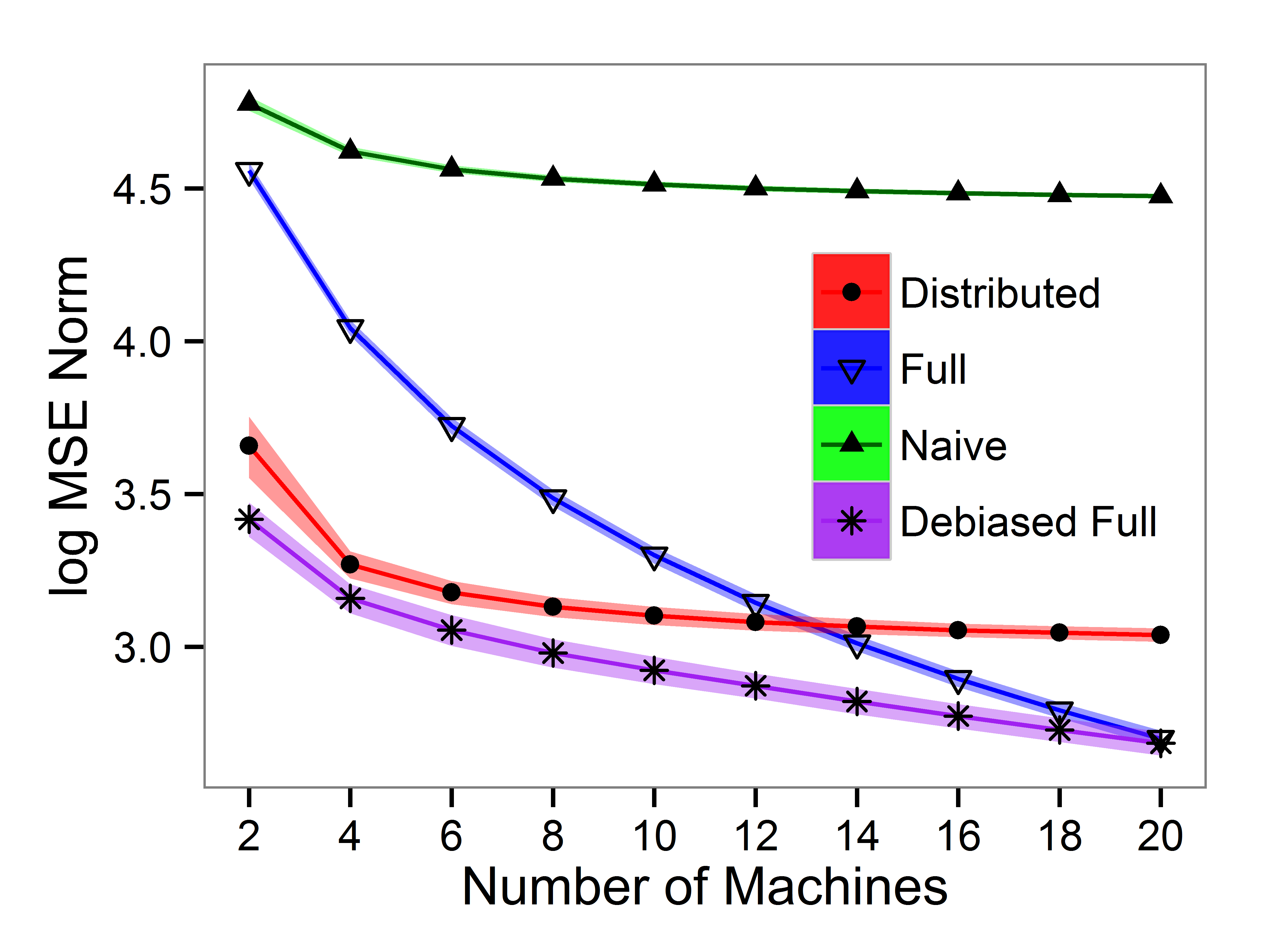
In Figure 1, the errors of the different estimators are shown. In general, a better estimator can be obtained using the full data, which is expected. However, when the number of machines is small, the performance of our distributed estimator is comparable to the estimators on the full data, both in mean squared error and $\ell_{\infty}$ norm. In mean squared error, when $M$ is small, the debiased estimators perform better because they trade off bias for variance. Thus, Debiased Full performs the best and Distributed has similar performance. Naive performs poorly under this norm for all $M$. In $\ell_{\infty}$ norm, the performance of Full and Full Debiased is exactly the same because the largest error is from the entries in the diagonal, which are equal since the diagonal is not penalized. The error of Distributed is approximately the same for a wide range of values of $M$. However, in $M=2$, the performance of Distributed is affected by the bandwidth since missing edges in any machine have a larger impact on the error. But as the number of machines increases, the estimation of Distributed becomes insensitive to the bandwidth.

To evaluate the robustness of the method against the selection of the tuning parameters $\lambda$ and $\tau$, we measure false positive rate (defined as percentage of zeros of $\Theta$ identified as edges by the estimator) and false negative rate (defined as percentage of edges missed by the estimator). We use the same settings as the previous scenario, but the number of machines is fixed to $M=10$. The values of the tuning parameters for our method vary proportionally to $\lambda=\beta\sqrt{\log(p)/n}$ and $\tau=\beta\sqrt{\log(p)/(Mn)}$ with $\beta$ between $0.2$ and $2$. The bandwidth is still fixed at 1% of the entries. We observe that for a wide range of parameters we recover the correct set of non-zeros.

References

- [1] Onureena Banerjee, Laurent El Ghaoui, and Alexandre d’Aspremont, “Model selection through sparse maximum likelihood estimation for multivariate Gaussian or binary data,” The Journal of Machine Learning Research, vol. 9, pp. 485–516, 2008.
- [2] Jerome Friedman, Trevor Hastie, and Robert Tibshirani, “Sparse inverse covariance estimation with the graphical lasso,” Biostatistics, vol. 9, no. 3, pp. 432–441, 2008.
- [3] Stephen Boyd, Neal Parikh, Eric Chu, Borja Peleato, and Jonathan Eckstein, “Distributed optimization and statistical learning via the alternating direction method of multipliers,” Found. Trends Mach. Learn., vol. 3, no. 1, pp. 1–122, Jan. 2011.
- [4] John C Duchi, Alekh Agarwal, and Martin J Wainwright, “Dual averaging for distributed optimization: convergence analysis and network scaling,” Automatic control, IEEE Transactions on, vol. 57, no. 3, pp. 592–606, 2012.
- [5] Yuchen Zhang, John C. Duchi, and Martin J. Wainwright, “Communication-efficient algorithms for statistical optimization,” J. Mach. Learn. Res., vol. 14, no. 1, pp. 3321–3363, Jan. 2013.
- [6] Jason D. Lee, Yuekai Sun, Qiang Liu, and Jonathan E. Taylor, “Communication-efficient sparse regression: a one-shot approach,” ArXiv e-prints, Mar. 2015.
- [7] Adel Javanmard and Andrea Montanari, “Confidence Intervals and Hypothesis Testing for High-Dimensional Regression,” ArXiv e-prints, June 2013.
- [8] Zhaoshi Meng, Dennis Wei, Ami Wiesel, and Alfred O Hero, “Marginal likelihoods for distributed parameter estimation of Gaussian graphical models,” Signal Processing, IEEE Transactions on, vol. 62, no. 20, pp. 5425–5438, 2014.
- [9] Adam J. Rothman, Peter J. Bickel, Elizaveta Levina, and Ji Zhu, “Sparse permutation invariant covariance estimation,” Electron. J. Statist., vol. 2, pp. 494–515, 2008.
- [10] Pradeep Ravikumar, Martin J. Wainwright, Garvesh Raskutti, and Bin Yu, “High-dimensional covariance estimation by minimizing l1-penalized log-determinant divergence,” Electron. J. Statist., vol. 5, pp. 935–980, 2011.
- [11] Jana Janková and Sara van de Geer, “Confidence intervals for high-dimensional inverse covariance estimation,” Electron. J. Statist., vol. 9, no. 1, pp. 1205–1229, 2015.
- [12] Tuo Zhao, Han Liu, Kathryn Roeder, John Lafferty, and Larry Wasserman, “The huge package for high-dimensional undirected graph estimation in R,” The Journal of Machine Learning Research, vol. 13, no. 1, pp. 1059–1062, 2012.