Relating Transverse Momentum Dependent and Collinear Factorization Theorems in a Generalized Formalism
Abstract
We construct an improved implementation for combining transverse-momentum-dependent (TMD) factorization and collinear factorization. TMD factorization is suitable for low transverse momentum physics, while collinear factorization is suitable for high transverse momenta and for a cross section integrated over transverse momentum. The result is a modified version of the standard prescription traditionally used in the Collins-Soper-Sterman (CSS) formalism and related approaches. We further argue that questions regarding the shape and -dependence of the cross sections at lower are largely governed by the matching to the -term.
I Introduction
Much of the literature on the TMD-factorization formalism is based on methods like those of Collins Soper and Sterman (CSS) [1, 2, 3, 4] where, traditionally, applications have been at very high scales. The formalism involves a factorization with TMD parton densities and/or fragmentation functions together with evolution equations and associated properties like universality. TMD correlation functions have attracted interest, both for their usefulness in perturbative calculations, and for their potential to yield information about underlying non-perturbative QCD structures. Results with essentially the same or a related structure are also found in SCET [5, 6, 7]. In this paper, we focus on the CSS formalism and its updated version in Ref. [4].
TMD correlation functions are most useful for , where is the relevant transverse momentum and is the overall hard scale. When is of order , the cross section does not factor into TMD correlation functions, but normal collinear factorization applies. It is, of course, necessary to be able to analyze cross sections over the whole range of including intermediate transverse momenta. To this end, CSS organized the cross section into an additive form, , where is the pure TMD factorization term and is a correction term using collinear factorization. dominates in the limit of small while is a correction for large . This was designed with the aim to have a formalism that is valid to leading power in uniformly in ; here is a typical hadronic mass scale.
However, it has become increasingly clear that the original CSS method is not sufficient for modern TMD applications. One reason is that there is a growing number of lower- phenomenological studies focused on the intrinsic transverse motion related to nonperturbative binding and nucleon structure. The advantages of the usual decomposition are clearest when is large enough that there is a broad intermediate range of transverse momentum characterized by ; that is, there is a range where is sufficiently small that TMD factorization is valid to good accuracy, while is also sufficiently small that collinear factorization is simultaneously valid. However, at lower phenomenologically interesting values of , neither of these ratios is necessarily very small. Some other difficulties will be summarized below. These particularly concern the ability of the original method to properly match collinear factorization for the cross section integrated over .
The problems create practical difficulties for studies specifically devoted to extracting and analyzing non-perturbative transverse momentum dependence. For such applications, the relevant experiments often involve hard scales of only a few GeV. The phase space of has a narrow transition window between a solidly perturbative transverse momentum region (where ) and a non-perturbative region (where ), making the treatment of matching the perturbative and nonpertubative content in the intermediate region rather delicate. A classic analysis of the issues concerning the matching of the TMD factorization and collinear factorization was given by Arnold and Kauffman [8], and more recently in Refs. [9, 10, 11, 12]. See especially Sec. 2.6 of Ref. [9] for a recent overview of many of the issues to be discussed in this paper.
Over the past several years, most theoretical attention in TMD physics has been focused on the details of evolution of the -term and its associated TMD correlation functions. However, particularly with recent results like [10, 11, 12], it is evident that a satisfactory treatment of non-zero corrections and the matching to is important since it relates various phenomenological analyses to TMD theory. This is especially the case in efforts to interpret transverse momentum spectra in terms of hadronic structure, where a detailed separation and identification of large and small behavior and its potential interplay is important.
Generally, to get results that are valid over all we need to combine the information given by TMD factorization and by collinear factorization. TMD factorization is appropriate for ; its accuracy degrades as increases and eventually it does not give even a qualitatively correct account of the cross section. Collinear factorization is valid in two ways. One is for the cross section differential in with ; the accuracy degrades as decreases, and collinear factorization becomes entirely inapplicable for the differential cross section once is of order or smaller. But collinear factorization is also valid for the cross section integrated over .
In this article, we argue for an enhanced formalism. As already stated, the formalism as given by CSS was designed to combine the best of TMD and collinear factorization at intermediate . What was not done was to adjust the formalism to work nicely also for the cross section integrated over all . We summarize an interconnected set of problems as follows:
- •
A standard way of presenting the term, with the solution to the evolution equations, is as a Fourier transform from a transverse coordinate to transverse momentum. When , the -space integrand goes to zero. (See Appendix A.) Therefore, the integral over all transverse momentum of the corresponding momentum-space contribution is zero. Now, at small , is the dominant TMD-factorized contribution to the cross section, and is necessarily positive. Therefore, at some larger , the term must become negative. By construction, the term compensates to give the physical positive cross section, so this is not a problem in principle. However, if becomes large and negative at , the term becomes large and positive, so the formalism involves implementing a cancellation of two large quantities. This can enormously magnify the effects of truncation errors in perturbative quantities, since these have different structures in and .
- •
In pure parton-model treatments of TMD functions, the transverse momentum integral of the -term gives the collinear factorization parton model for the cross section integrated over . The previous item shows that, at least within the original CSS approach, this connection is not merely subject to higher-order perturbative corrections, but is totally lost.
- •
In real QCD, consider the cross section integrated over all ; it is of the form of factors of collinear parton densities and/or fragmentation functions at scale convoluted with hard scattering that is expanded in powers of . The lowest order for the integrated cross section itself is correctly given by a perturbative expansion of the hard scattering, with the first term being zeroth order in (concentrated at ). We can try doing this for all quantities in
(1) Since the integral over is zero, the integrated cross section is given by the integral over of the term. But the CSS construction of the term shows that its lowest term is the same order as for collinear factorization for the differential cross section, which is first order in [3] .
We thus have a paradox: a mismatch of orders in between the left and right hand sides of Eq. (1). The real source of the paradox and an indications of what to do about are indicated next.
- •
The zero value of is not obtained from a fixed order perturbative application of collinear factorization to at , but from the solution of evolution equations for , as seen in Eq. (35) below. Each order of the perturbative expansion in powers of contains up to two logarithms per loop of . These logarithms are evidently infinite at , and fixed order perturbative calculations are entirely inapplicable to with the original CSS definition.
Recall that is an approximation to the cross section only for . Thus the transverse-coordinate-space quantity is important for a physical cross section only for bigger than about . Finite perturbative orders of the collinear expansion are useful when is of order .
- •
Even without the issue of becoming negative at large , there is the issue that it involves, in momentum space, a convolution of two independent TMD densities. At large , these can be computed perturbatively in terms of collinear parton distribution functions (pdfs) and/or collinear fragmentation functions (ffs). Power counting indicates that they are roughly of order . Therefore, the basic TMD factorization formula gives a cross section that has this same power counting, and extends infinitely far beyond the kinematic limit. The term compensates this in principle, but the different perturbative truncations in and imply that the result can be numerically a bad approximation.
The culprit in each of the above is that the TMD factorization formula used in was derived to be a good approximation to the cross section for , but in the integral over , the formula is being used far beyond its domain of applicability.
There is a uniqueness to the particular form of that gives rise to its undesirable properties at large . The uniqueness arises from the use of a strict leading power expansion in when constructing the TMD factorization formula for . As an illustration, consider a lowest-order perturbative expansion that gives in a factor at small , with its characteristic logarithm. The use of exactly a single power of (times logarithms) entails keeping the same formula at large , where the logarithm becomes negative.
The use of a strict leading power in is is important because the non-leading powers are much more complicated and often non-factorizing. This issue is particularly important because, to leading power, gluons can connect subgraphs in different kinematic regions. To get factorization, Ward identities are used to extract these gluons into attachments to Wilson lines in operator definitions of the correlation functions like TMD pdfs and ffs. However, the Ward identities apply only in the context of an approximation that is valid at leading power (or perhaps one power beyond). The result is the afore-mentioned uniqueness in the factorized form. Essentially the same considerations apply in SCET for essentially the same reasons — see Ref. [7].
It therefore becomes quite non-trivial to adjust the TMD factorization formula to get nicer properties at large without violating the derivation of TMD factorization.
Many implementations of TMD factorization calculate TMD functions by effectively resuming logarithms of . The usefulness this type of resummation assumes that there is a broad range of where . At smaller the window satisfying this condition shrinks and eventually vanishes, so that the advantage of such techniques becomes questionable. Moreover, errors introduced by including the region where can start to become a significant fraction of the resummation calculation.
The situation is simpler if one simply works in a leading logarithm approximation as in the work of Parisi and Petronzio (PP) [13]. There an ad hoc modification to impose rough approximations to the true kinematics is appropriate. But modifications are much harder to impose in the middle of a full proof of factorization that is to be applied generally.
Our approach in this paper is to preserve the factorized form of in transverse coordinate space, but to modify the way in which it is used to construct a contribution from to the cross section, to try to evade the problems listed above. We must preserve the property that gives a good approximation to the cross section at low transverse momentum, including the important region where is in the non-perturbative region of order . Naturally, the definition of must be correspondingly modified.
The paper is organized as follows: We provide a general background of the main issues in Sec. II, and outline the principles that will guide our matching procedure. We review the basic logic of the method in Sec. III, and include some clarifying remarks. Since an important component of our procedure is that it leaves the treatment of the -term largely unaltered, we will also need to review the standard factorization and evolution of the -term in the CSS TMD factorization formalism, which we do in Sec. IV. Next, we will explain our modifications, starting in Sec. V with a modified treatment of the standard -prescription. This will allow us to construct a generalized -term. From this we will obtain a correspondingly generalized -term in Sec. VI. Thus we will have constructed a new method, but with additional parameters. In Sec. VII we discuss how the principles from Sec. II constrain parametrizations. In Sec. VIII, we elaborate on technical steps needed to calculate in the new prescription, and in Sec. IX we demonstrate the utility of our treatment by calculating the term with simple parametrizations of collinear quark pdfs and ffs. We conclude by summarizing our logic and commenting on ways forward in Sec. XI.
II Guiding Principles
The standard construction relies on the fact that, at very large , there is a broad range where and are both good small expansion parameters. We suggest the following principles to guide the choice of an improved formalism:
- 1.
When the term is integrated over all , it should obey an ordinary collinear factorization property. This implies that when the scales in the pdfs and ffs are set to , the result should agree with the ordinary factorization calculation for the integrated cross section to zeroth order in , thereby matching the parton-model result appropriately.
- 2.
For , the cross section given by should appropriately match fixed order collinear perturbation theory calculations for large transverse momentum.
- 3.
For very large , the normal construction should automatically be recovered for the region, to leading power in .
- 4.
The modified term should be expressed in terms of the same coordinate space quantity as before, in order that operator definitions of the pdfs and ffs can be used, together with their evolution equations.
- 5.
The sum should give a leading power approximation to the cross section over the whole range of . Fixed order expansions of in collinear perturbation theory are suitable for calculating , while the usual solution of evolution equations is used for .
We will use these principles to strongly motivate our new constructions of and .
We emphasize here that many of the elements of this article have already been used in the past in various forms. Our purpose in this paper is to synthesize and systematize them.
For example, a detailed discussion of large and small matching and the associated perturbation theory errors in intermediate regions of appears in Ref. [8] – see especially Sections 1.2-1.4 for a clear discussion. The work of Catani-Trentadue-Turnock-Webber and related treatments, especially Bozzi-Catani-de Florian-Grazzini (BCFG) in [14] replace terms in a resummation with , thus cutting off the contribution. This is similar to work by Parisi and Petronzio [13] that used this method to handle the region in a leading-log approach. BCFG also impose constraints on the relationship between integrated and transverse momentum dependent cross sections that are very similar to our points 1) through 3) above.
Nadolsky, Stump and Yuan (NSY) [15] performed a CSS-style analysis of semi-inclusive deep inelastic scattering (SIDIS), but modified the large behavior of their resummed term by introducing corrections to the and kinematic variables. Specifically, NSY modified the -term at larger values of to improve matching asymptotic term as order corrections start to become large. By examining the kinematics of the process, they found that an improved matching is achieved if one replaces the standard and variables in the collinear pdfs and ffs of the term by11 1 See the discussion regarding matching in Section VA of Ref. [15] and the comparison between the modified and unmodified treatments in Fig. 9 of Ref. [15].
| (2) | ||||
| (3) |
In Ref. [4, Eq. (13.75)], Collins proposed to impose a direct cutoff on the large part of the -term. Our method follows a very similar approach (see Sec. V), with our function in Eq. (38) corresponding to Collins’s , and our corresponding roughly to Collins’s . Likewise, CSS introduced a mass-scale in Ref. [3] to regulate the low part of the -term calculation. The role of is analogous to what we will call in Sec. III. The replacements in Eqs. (2)–(3) are physically motivated in that they approximate the kinematic corrections on and momentum fractions that begin to be important at larger . See also Sec. 2.6 of Ref. [9] for a review of the kinematical rescaling procedure.
In most implementations of the ResBos Monte Carlo, for both Drell-Yan and SIDIS, the computational algorithm automatically forces a switch between the -term (there called the “resummed term”) to a calculation done using purely fixed order perturbative QCD above some . In fact, this is useful also for improving the efficiency of computer calculations since it means that computationally intensive calculations of the -term can be short circuited above some without compromising the accuracy of the calculation. (See Refs. [16, 15].) For very low , the ResBos Monte Carlo switches off the -term for GeV [17].
Boer and den Dunnen [18, 12] used a method similar to BCFG, but implemented the transition to very small by using a modified renormalization group scale (called ). This aspect of the Boer-den Dunnen approach is very similar to what we will use in this article.
We suggest that, to maintain context, it will be useful to read the articles listed above concurrently with this paper.
III and Terms
We start by reviewing the construction. This will establish notational conventions to be used throughout the paper in addition to clarifying the logic of the method. We will also introduce one of our modifications.
Consider a generic transverse momentum dependent cross section that depends on a hard scale and is differential in a transverse momentum . It may also be differential in other kinematical variables, but for simplicity we will not show these explicitly. It could be any cross section for which a TMD factorization theorem exists. We will use the abbreviated notation
| (4) |
The ellipsis indicates possible dependence on other kinematical variables like and , whose exact values are not relevant to our immediate discussion. Although the logic in this paper is meant to apply generally, explicit expressions will be written for SIDIS. CSS-style derivations of TMD factorization are given for SIDIS in Refs. [19, 20] (see also [4, Sec. 13.15]).
The TMD formalism separates Eq. (4) into a sum of two terms. One term () describes the small transverse momentum behavior and an additive correction term () accounts for behavior at :
| (5) |
The first term on the right is written in terms of TMD pdfs and/or TMD ffs and is constructed to be an accurate description in the limit of . It includes all non-perturbative transverse momentum dependence. The -term is described entirely in terms of collinear factorization. Our aim is to construct and such that gives the cross section up to an error that, relative to the cross section, is of order a positive () power of , where is a hadronic mass scale.
The original CSS definition of is as given in, for example, Ref. [4, 13.71] (where it is called ):
| (6) |
The “approximator” is an instruction to replace the object to its right by an approximation that is designed to be good in the limit. That is, it replaces the exact by the approximate :
| (7) |
where .
Another approximator, , handles the large region. It replaces with an approximation that is good when . That is,
| (8) |
where . Since is to be applied to the region, one only needs collinear factorization at a fixed order and with a hard scale .
If and were the only regions of interest, then the and approximators would be sufficient. One could simply calculate using fixed order collinear factorization for the large -dependence and TMD factorization for small -dependence. A reasonable description of the full transverse momentum dependence would be obtained by simply interpolating between the two descriptions [21, 22].
However, the region between large and small needs special treatment if errors are to be strictly power suppressed point-by-point in . The standard method is to construct a sequence of nested subtractions. The smallest-size region is a neighborhood of , where gives a very good approximation. So, one starts by adding and subtracting the approximation:
| (9) |
From Eq. (7), the error term in the square brackets is order and is only unsuppressed at . Therefore, one may apply and then use a fixed-order perturbative expansion in collinear factorization:
| (10) |
where . Thus, the cross section is determined point-by-point in the mid- region, up to powers of , by a combination of TMD and collinear correlation functions.
The CSS construction of defines and to be the first and second terms on the second line of Eq. (10). Their specific definitions of and allowed Eq. (10) to work only in the region, which we emphasize by the argument on the left side of Eq. (10). The error estimates in Eq. (10) are inapplicable outside this range, i.e., they must not be applied when or . This is because they were extracted from the leading power of expansions in relatively small kinematic variables and to give Eqs. (7) and (8). The issues are illustrated by Eq. (8). The estimate is obtained from an expansion in powers of mass with respect to the smallest scale in the collinear hard-scattering; it is of the order of the first omitted term in the expansion. But once gets much smaller, the error can be arbitrarily larger. As a mathematical example, suppose
| (11) |
The leading power expansion in is
| (12) |
and the error is
| (13) |
For the error estimate when , we can correctly take :
| (14) |
But when , the error is a stronger behavior, relative to .
It is useful to review the precise meaning of notation in the error estimates, which is as follows: An error means that there exist constant positive real numbers, and , such that the error is less than for . Analogous statements apply to and error estimates. Thus, the error estimates in Eqs. (5)–(10) provide no constraints on the behavior in the or regions. As shown above, the true errors in those regions could be much worse than a naive extrapolation of the powers in Eqs. (5)–(10) would suggest.
The above observations do not represent a fundamental breakdown of the formalism. They merely indicate that some extra care is needed to construct a formalism valid also for and .
For , collinear factorization is certainly not applicable for the differential cross section. But this region is actually where the -term in Eq. (7) has its highest validity. So one simply must ensure that the would-be -term
| (15) |
is sufficiently suppressed in Eq. (10) for . Therefore, we will modify the usual definition of by inserting a suppression factor at low :
| (16) |
The smooth cutoff function approaches zero for and unity for . It ensures that the -term is a correction for only. As long as , any -dependence must be weak. This is analogous to the introduction of a in Ref. [3, Eq. (2.8)].
The exact functional form of is arbitrary, but is most useful in calculations if it sharply suppresses contributions while not affecting . While a step function is acceptable, we suggest using a slightly smoother function since one expects the transition from perturbative to non-perturbative physics to be relatively smooth. One possible choice is
| (17) |
This is what we will use in sample calculations in Sec. IX. A large value for the power makes the switching function more like a step function.
In common terminology, the first term in braces on the second line of Eq. (16) is called the “fixed order” (FO) contribution, while the second term is the “asymptotic” (AY) contribution. We will use the notation
| (18) | ||||
| (19) |
So,
| (20) |
This corresponds to the terminology in, for example, Ref. [15]. The term “fixed order” is meant to imply that the calculation of is done entirely with collinear factorization with hard parts calculated to low order in perturbation theory using and with collinear pdfs and ffs calculated using . That is, the hard part and the parton correlation functions are evaluated at the same scale.
Now we can extend the power suppression error estimate in Eq. (10) down to to recover Eq. (5). Equation (10) becomes
| (21) |
which is Eq. (5), but restricted to .
So far, aside from introducing an explicit , we have only reviewed the standard construction. The restriction on the left of Eq. (21) should be emphasized. Since we rely on strict power counting in and , the region of is not guaranteed to be well-described by the above construction. We will correct this in Secs. V–VII with a modified -term definition.
IV Review of TMD Factorization and Basic Formulas
Our proposed modifications to the transition to the region will leave the standard treatment of TMD factorization [4, Chapters 10,13,14] in the region only slightly modified.22 2 See also Ref. [23] for a recent brief overview and large list of references relating to the development of TMD factorization. In particular, the operator definitions for transverse-coordinate-space TMD functions, along with their evolution properties, are exactly the same as in the usual formalism. This is an important aspect of our suggested modifications, so it is worthwhile to review the basics of TMD factorization for the low region. This section gives a short summary of the most important formulas, with the organization of notation optimized for discussions in later sections. We will also refer frequently to the review of TMD evolution in Ref. [24, Sec. II], especially [24, Eqs. (22, 24)].
IV.1 TMD Evolution
The evolution of follows from generalized renormalization properties of the operator definitions for TMD pdfs and ffs. To separate perturbative and non-perturbative contributions, one defines large and small through a function that freezes above some and equals for small :
| (22) |
The relevant renormalization group scales are
| (23) |
where and are constants that are chosen to optimize perturbative convergence.
We first solve the evolution equations, to give the following forms for the -term for SIDIS (neutral-current and neglecting heavy flavors):
| (24) |
Here , and are, respectively, the TMD pdf and TMD ff evaluated at a reference scale . Their operator definitions are given in Eqs. (13.42,13.106) of Ref. [4]. The exponential factor on the second line implements the evolution from to . There is the Collins-Soper (CS) evolution kernel (see [24, Eq. (6,11,25)]), while and are anomalous dimensions for the CS kernel and a TMD pdf/ff respectively (see [24, Eq. (7,8,9,10,12)]). See also Refs. [23, 25] and references therein for detailed discussions of the evolution equations and their origins. In the last part of Eq. (24), we have used the renormalization group to change the argument of from to . This is in anticipation of later manipulations, where will be a suitable scale for perturbatively calculated quantities.
We define the -space version of the -term by
| (25) |
To economize notation, we will assume there is only one flavor of parton so that we may drop the sum over and the subscript. In detailed calculations, the sum needs to be restored.33 3 Recall, however, that for scattering off a quark, there is no flavor dependence in the hard scattering until order . So flavor independence is likely a good approximation. See the discussion at the beginning of section VIA of Ref. [24].
In the limit , each TMD correlation function can be expanded in an OPE and expressed in terms of collinear correlation functions. Then the transverse coordinate dependence is itself perturbatively generated. Let us define a notation to describe this limit. First, substitute in Eq. (24) to regulate the region. Second, expand the result in an OPE and drop order corrections. Finally we replace and by , so that perturbatively calculations have no large logarithms. We call the result :
| (26) |
The functions and are the ordinary collinear pdf and ff. Equation (26) is the standard result for the small limit and corresponds to Eq. (22) of Ref. [24], but without the non-perturbative exponential factors. Thus,
| (27) |
with .
IV.2 Separation of Large and Small
For Eq. (22), a common functional form is [26]:
| (28) |
The standard steps for separating large and small are to first write a ratio,
| (29) |
The ratio on the right side defines the exponential functions on the left according to some reference scale . The -functions, therefore, account for all the error terms on the right side (27) (at some ).44 4 It is essentially just convention that the -functions appear in an exponent. Next, one notices that the CS evolution is identical for the numerator and denominator, apart from the fact that the evolution kernel is evaluated at in the former and in the latter. Thus, one may re-express the right side of Eq. (29) in terms of at an arbitrary in a very simple form by applying CS evolution to the numerator and denominator separately and canceling out many common evolution factors. The result is
| (30) |
Here, is the difference between the CS evolution kernels evaluated at and :
| (31) |
Now the kernel is very strongly universal; it is independent not just of the process, but also of scale, polarization, , , flavors, and polarization. The “non-perturbative” function , defined by Eq. (31), inherits the same strong universality properties as .
Equation (30) allows us to write
| (32) |
where is the combination of all non-perturbative exponential functions in Eq. (30),
| (33) |
is a function to be parameterized and fit to data, or to be determined by appealing to non-perturbative methods.55 5 To call , , and functions “non-perturbative” is somewhat of a misnomer. The definition of is indeed such that it does include all the strongly non-perturbative contributions. But if is conservatively small, also includes contributions, at moderate , that could be estimated perturbatively. is calculable in collinear factorization in terms of collinear pdfs and ffs and allows the use of low order perturbation theory for perturbatively calculable parts. It is exactly the original definition of , but evaluated at instead of . The exponential factors in Eq. (33) account for the non-perturbative transverse coordinate dependence. Notice that by construction
| (34) |
Substituting Eqs. (26) and (33) into Eq. (32) produces the most familiar representation of the evolved :
| (35) | |||||
This now includes all the necessary non-perturbative functions and corresponds to Eq. (22) of Ref. [24]. In the case that non-perturbative functions are dropped, the -term matches Eq. (1.1) of Ref. [3].
With the method of Eqs. (28)–(35), the relationship between and and the exact definition of from the factorization derivation is kept explicit. Equation (30) is exact because the evolution is the same for the numerator and denominator. Therefore, all corrections in Eq. (27) are accounted for automatically in the definition of the non-perturbative parts in Eq. (33). The only errors in the relationship between the -term and the physical cross section are the overall -suppressed errors from the factorization derivation.
This section has been a compressed review of steps already reviewed recently in Sec. 2.B.III of Ref. [24]. We refer the reader to this and references therein for more details.
V Modified -prescription and -Term
Next, we modify the definition of . This is to provide a convenient solution to the problem that with the definitions given so far, the integral over all of is zero, because is zero at (see App. A).
It would be preferable for the integral to have a normal collinear expansion in terms of pdfs and ffs at scale ; the lowest order term then reproduces the lowest order collinear factorization result for the integrated cross section. At the same time, we wish to preserve the results for the -space quantity , since these embody the derived factorization and evolution properties. Most importantly, the modified term must still approximate the cross section at low to the same accuracy as in Eq. (7).
We achieve the modified in two stages.
The first is to modify the Fourier transform in Eq. (25) to read
| (36) |
where
| (37) |
That is, is replaced by . The function is arranged to agree with when , but to be of order when , , thereby providing a cutoff at small . Then, when (36) is integrated over , we get , instead of the previous value . We have included an explicit numerical factor of since this tends to lead to simpler formulas later on. We have chosen the value of to be proportional to , so that, from Eq. (35), has a normal collinear factorization property. The numerical constant fixes the exact proportionality between and .
But at the same time (36) still gives an approximation to the cross section of the appropriate accuracy. This is because, when , the dominant range of is much larger than , and so the modification in (36) only gives a power-suppressed contribution. Of course, at large , there are more substantial changes. But then we approach the domain of validity of collinear factorization, and so the accuracy of the form is preserved provided that, in the definition (16) of , we replace by .
Note that the integrand in (36) is non-singular at , unlike (25). Thus the large behavior is exponentially damped. Even so, the function still extends to arbitrarily large .
So the second and final stage of modification for is to make an explicit cutoff at large , to give:
| (38) |
Here is a cutoff function that we introduce to ensure that vanishes for , and is a parameter to control exactly where the suppression of large begins. should approach unity when and should vanish for . This preserves the required approximation property of at small . At the same time, since the changes are dominantly at large , the integral over all still has a normal collinear expansion, as we will make more explicit below.
A simple step function is acceptable for . When we combine with a -term in Secs. VI–VII we will introduce methods to minimize sensitivity to the exact form of . However, a smoother function is preferred since the domain of validity of the -term approximation does not end at a sharp point in , and thus a smooth function characterizes general physical expectations. A reasonable choice is
| (39) |
with .
The only differences between the old and new -term are: i) the use of rather than in , and ii) the multiplication by . (The second modification was proposed by Collins in Ref. [4, Eq. (13.75)]. There is called .) Equation (38) matches the standard definition in the limit that and approach infinity.
Finally, we will present a fully optimized formula for corresponding to the one for the original in Eq. (35).
But first it will be convenient to construct some auxiliary results.
Naturally, is to be replaced by
| (40) |
Also we define
| (41) |
Then, for large enough and
| (42) |
Thus, decreases like , in contrast to which remains fixed. Note also that
| (43) |
For , . Instead of , we will ultimately use the scale
| (44) |
to implement renormalization group improvement in TMD correlation functions. There is a maximum cutoff on the renormalization scale equal to
| (45) |
The approximation sign corresponds to the limit of large . Note that,
| (46) |
The steps for finding a useful formula for the evolved are as follows. Equation (32) becomes
| (47) |
Now the definition of is unchanged, and only the replacement is new. Therefore instead of Eq. (35) we simply need
| (48) | |||||
This is the same as Eq. (35) except that and are used instead of and . Note that depends on through , albeit only for . For , . Also, does not vanish exactly as but instead approaches a power of .
Up to this point, we have introduced two new parameters, and , in the treatment of the -term.
VI Modified -Term
Now we can construct a -term from nearly identical steps to those of Sec. III. Recall that the TMD approximator, , replaces the cross section by an approximation that is good in the limit – see Eq. (6). The from Ref. [4] replaces by the definition of that follows most directly from the derivation of TMD factorization. However, any approximator that is good when is equally valid here. Therefore, we write
| (49) |
Here applies the same approximations as , but with the use of and as in Eq. (38).
Since the changes only affect the region , power counting for small proceeds in exactly the same way as in Sec. III:
| (50) |
The large region is dealt with using the same approximator as in Sec. III:
| (51) |
Continuing the usual steps, a -term is constructed by adding and subtracting :
| (52) |
The term in brackets is only unsuppressed for large , so we apply to it the large approximator, , and use collinear factorization:
| (53) |
where .
Finally, we insert a factor of the function from Eq. (16) to remove any -term contribution in the region. The final -term is
| (54) |
Then,
| (55) | ||||
| (56) |
So,
| (57) |
As usual, is an instruction to set all renormalization scales to and drop powers of or . In , the inserts a multiplication by a factor of , effectively setting to zero for large (see, e.g., Eq. (39)). Thus, if gets dropped when is applied, there is a potential to introduce large errors. Therefore, should not drop the factor of because , by definition, must leave the region unmodified. Similarly, the use of affects the small limit of , and therefore can also have a large effect on on at large . Thus, should preserve the use of . In contrast, mainly affects the small region. Therefore, we define to apply the limit in Eq. (56). Examples of implementations of Eqs. (55)–(57) will be given in Secs. VIII and IX.
Now observe that approaches zero as gets much larger than . Then approaches the usual collinear factorization result for at large . Therefore, we may at last remove the restriction on the left side of Eq. (21) and write a representation of the cross section that extends over the whole range of :
| (58) |
We have reached our goal of constructing a expression that does not require that we specify limitations on the range of . What remains is to determine the most appropriate values for and .
VII Connection with -integrated cross sections and collinear factorization
In this section, we analyze the integral over all of the right-hand side of Eq. (58), and show how it matches standard collinear factorization for the integrated cross section.
We integrate Eq. (58) over all transverse momentum, and then reorganize the result as follows:
Term 1 is integrated over , but without the factor, so it can easily be simplified. Term 2 corrects for the omission of , while term 3 is the integral of the term.
Now term 1 equals . Since , we can replace it by the OPE form, to leading power in , Eq. (27), to obtain
| (60) |
Then, we can use Eq. (26) to give a factorization in terms of collinear pdfs and ffs at a scale of order . Since in that formula is replaced by , while is of order , both the factors and the quantities in the exponential can be expanded in powers of without large logarithms. We therefore have a normal collinear expansion. The lowest-order term gives
| (61) |
with our choice of scale given in Eq. (45). This agrees with the lowest-order term for the integrated cross section itself, i.e., for .
Both terms 2 and 3 are dominated in their integrals by of order . They therefore have normal collinear expansions, starting at order . Overall, we therefore have well-behaved perturbative expansions of collinear factorization for each term, unlike the case for the integrals of the original CSS forms for and .
We now show more explicitly that terms 2 and 3 are dominated by of order . For term 2, the factor gives a power suppression for , while the use of instead of gives an exponential suppression for , as we have already seen. For term 3, the construction of gives power suppression when , with the factor in (57) ensuring that no pathologies arise when is very small (below ). At large , beyond , the term obeys the kinematic limit, while the term is exponentially suppressed, for the same reason as for .
VIII Calculating the asymptotic term in the BCFG method
Perturbative calculations for the hard coefficient for the term in the original CSS version can be performed by starting from the normal collinear coefficient for the cross section as a function of . Then the asymptote at small is subtracted. This asymptote is simply the leading power expansion in when is much smaller than , and involves simply a factor of time logarithms of in each order of perturbation theory. The coordinate-space version of the subtraction in each order is correspondingly a polynomial in .
In the new scheme, the coordinate space formula is unchanged, but it is not so simple to perform a practical analytic calculation of its Fourier transform to give . This is because of the substitution of for . We now explain how to do this, following Ref. [14].
Calculations of need Fourier-Bessel transforms of terms of the form
| (62) |
with and and . (The use of in the argument of the logarithm is a convention that typically results in simpler formulas.) These terms arise from the perturbative expansion . This can be considered as arising from the collinear factorization of Eq. (26) with replaced by , with all couplings expressed in terms of , and then with a fixed-order perturbative expansion applied to the product of the factors and the exponential in Eq. (26).
If , then we neglect the second term in the logarithms, and Eq. (62) becomes the much more familiar form from standard CSS-like treatments
| (63) |
VIII.1 Standard Logarithms
In the CSS and related treatments, with the standard construction, the logarithms are of the form of Eq. (63). In that case, the momentum space expressions are well-known (see, e.g., Eq. (36) of Ref. [15]). After Fourier transformation, coordinate space logarithmic terms like Eq. (63) give -dependence like
| (64) |
where the “” refers to higher power logarithms.
VIII.2 Modified logarithms
A primary motivation for our modified construction is to accommodate a non-zero in Eqs. (47) and (48), and thus a non-zero in Eq. (62). Fortunately, for the case of non-zero , analytic expressions for the finite parts of the Fourier-Bessel transforms have been worked out in Appendix B of BCFG, Ref. [14]. Indeed, the case of of corresponds exactly to the prescription of PP [13] and used in implementations like [14].
Now, the discussion so far has been based on the expression for in terms of TMD densities. However, to get the hard coefficient for , as needed in , it is also possible to start from the hard coefficients for ordinary collinear factorization for the cross section. Then one does the expansion at small to give times logarithms. Finally to obtain the effect of the use of instead of , one makes the substitutions given below.
One can read the substitutions off from results like Ref. [14, Eqs. (B.10)-(B.13)]. For example,
| (65) | ||||
| (66) |
Here, is the modified Bessel function of the second kind and
| (67) |
The left and right sides of Eqs. (65)–(66) are approximately equal for fixed and . See also the discussion around Ref. [14, Eq. (B.25)].
Now one may perform substitutions like Eqs. (65)–(66) to known results for the asymptotic term like Eq. (36) of Ref. [15] to obtain the generalized, non-zero , asymptotic term. Reference [14, Appendix B] contains results for any , so the modified asymptotic term, and thus the new -term, can be obtained to any order from previously existing expressions. For completeness, low order expressions for the asymptotic terms are given in Appendix B.
IX Demonstration
To illustrate the steps above, we have performed sample calculations of the -term using analytic approximations for the collinear pdfs and collinear ffs. For simplicity, we consider only the target up-quark channel, and for the running we use the two-loop -function solution and keep the number of flavors at since we are mainly interested in the transition to low . Thus we use GeV [27]. To further simplify our calculations, we use analytic expressions for the collinear correlation functions, taken from appendix A1 of Ref. [28] for the up-quark pdf and from Eq. (A4) of Ref. [29] for the up-quark-to-pion fragmentation function.
Due to these simplifying assumptions, the following should be regarded as a toy model calculation, meant to illustrate the basic steps of a -term calculation and to demonstrate plausibility for use in more complete and detailed calculations.
 |
| (a) |
 |
| (b) |
First, one must establish parameters for our large and small cutoff functions. For we use Eq. (17), and try since this gives a rapid but reasonably gentle suppression of small . The choice of should be such that it has reached unity at values of near the perturbative-nonperturbative transition, say, GeV. Thus, we choose GeV. The result is shown as the blue dashed curves in Figs. 1. To understand the plots, recall that is used to restrict to large the region where -dependence is calculated with collinear factorization at fixed order fixed in perturbation theory.
For we use Eq. (39). The value of controls how rapidly the contribution from the -term gets cutoff. For large , the transition can be rather smooth since there is a broad region where and overlap. In our example calculation, we find that works well. The value of should be chosen such that when is large enough that approximations that use might be considered suspect. For small , . We find that the transition between and occurs between about and if . These results for are shown as the tan curves in Figs. 1. To understand the plots, recall that the purpose of is to suppress the region of the -term where it fails to provide even a rough approximation.

 |
| (a) |
 |
| (b) |
Next, we examine the effect of varying on the calculation of the asymptotic term. Standard expressions for the asymptotic term can be found in, for example, Eq. (36) of Ref. [15]. We use these results, along with the substitutions in Eqs. (65)–(66), to plot the new asymptotic term of Eq. (56) for a range of values. The result is shown in Fig. 2, where we have temporarily set to in order to highlight the effect of varying . The results for and are shown. The standard CSS result, corresponding to , is also shown for comparison. In all of our calculations, . One can observe the approach to the CSS result as increases.
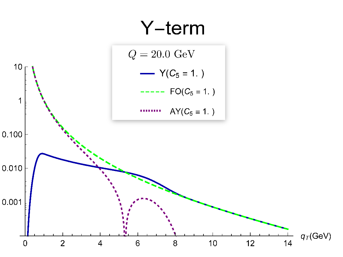
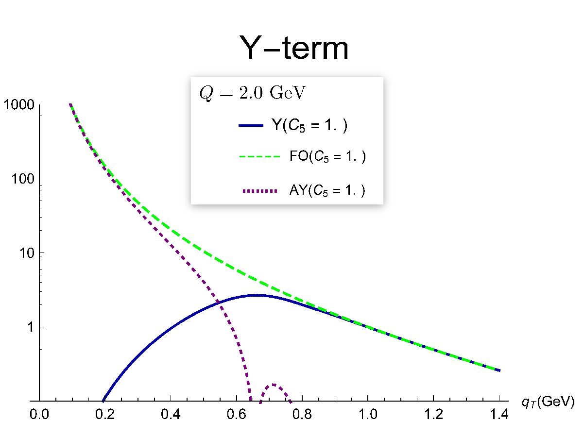
Finally, we restore the explicit in the asymptotic term and calculate the -term according to Eq. (57) for two values of , one large and one small. The results are shown in Figs. (3)(a,b). Here we use as a compromise between the various choices in Fig. 2 and to match with a common choice used in calculations like those of Ref. [14]. For GeV (Fig. 3(a)), there is a region where the -term is a useful non-trivial correction. Beyond about GeV, the -term simply approaches the calculation (where the -term vanishes).
Within our method, the -term remains a reasonable correction for large even down to GeV, as shown in Fig. (3)(b). There it forces a matching with the calculation at , while it vanishes for small .
Note that, if the entire range of up to order is considered, then the treatment of the -term plays an important role in describing the general shape of the -spectrum, particularly for the smaller values. Indeed, for smaller , the -term appears to dominate the tail region. These observations highlight the importance of achieving well-constrained collinear treatments of the large region. Most likely, calculations of the fixed order term to rather high order should be included in implementations to adequately describe the large behavior. For instance, Ref. [30] finds that order fixed order calculations are needed to get acceptable phenomenological success (see the comparison of curves in Fig. 4 of Ref. [30]). Reference [31] finds that threshold resummation corrections are also needed.
X Breakdown of Factorization in the Photoproduction Limit
 |
| (a) |
 |
| (b) |
 |
| (c) |
Of course, both TMD and collinear factorization theorems apply to the limit of a large hard scale ; part of the statement is that corrections to the factorized formulas are suppressed by powers of . Therefore, one expects factorization to work well in practice for very large and to fail completely for , with the in-between region being less clear. In the SIDIS case, the limit corresponds to photoproduction: . If is gradually decreased from some initially very large values, one expects uncertainties related to the general onset of non-perturbative physics beyond factorization to gradually increase.
This is, of course, a standard and well-known aspect of QCD. The most obvious signal of the breakdown of perturbative QCD factorization is that begins to blow up when . However, it is instructive to examine the transition from the solidly large region to the region in more detail. An analysis of the transition could guide applications of TMD factorization over a wide range of scales, aid in error analysis in applications, and provide intuition for how to match to truly non-perturbative physics. For example, in the true photoproduction limit, it may be useful to switch to a physical picture more closely resembling a Regge exchange model [32].
TMD factorization is most useful if there are distinct regions where i) , where TMD correlation functions can be used, and ii) , where collinear factorization applies. One way to test whether that is the case is to vary the parameter of Eq. (16). This controls the suppression of the -term for , so varying it should have small or negligible effects on how one treats the perturbative -dependence at .
Figure 4(a) confirms that this is true in our sample calculation for a very large value of GeV. The graph shows the -term for several values of along with the calculation (dashed) for comparison. The region where corresponds to a region where, roughly, . Therefore, one could probably rely mostly on the -term with its TMD pdfs and ffs to give a reasonable general description for . However, is still large enough in this region that power corrections to the -term might not be totally negligible, so the -term is a useful and important correction to a -term calculation in the moderate region. Including it can enhance precision over a wide range of . In the region the -term has negligible sensitivity to the exact value of (so long as ). The -term is, therefore, unambiguous in its region of relevance, up to choices in and . Moreover, variations in and can be understood in terms of higher order corrections. There is some residual sensitivity to for GeV, but for GeV, definitely corresponds to a region where . So, we are justified in simply ignoring the -term in the region.
In Fig. 4(b), we consider the lower value of GeV, where is relatively small, but still large enough to hope that TMD factorization is still useful. The range of as a fraction of is the same as in Fig. 4(a). For this smaller region, one might reasonably expect values of GeV to about GeV to qualify as . However, is still large enough here that concerns about power corrections from a -term are definitely warranted. As can be seen from the graph, the -term has significant uncertainties at intermediate when GeV coming from the exact choice of . Nonetheless, the region of GeV corresponds to , so in the the smallest region one may be confident in the applicability of factorization. Likewise, for GeV, one may begin relying on the calculation. Our construction interpolates between these two descriptions. Therefore, it is reasonable to expect a fit to GeV data to be qualitatively consistent with TMD factorization, even though uncertainties associated with -suppressed violations of factorization may begin to be more discernible. Said differently, at GeV, there may be a window of intermediate where and are not both simultaneously small, yet we obtain a reasonable overall description by calculating the behavior and the behavior and interpolating between the two. The only uncertainty then is in the exact nature or the interpolation. Notice, furthermore, that once a fit has been performed at GeV, any sensitivity to automatically vanishes after evolution to large , as illustrated by Fig. 4(a). In other words, there is no disadvantage to optimizing fits at liberally low since the limiting behavior at large is unaffected.
To see the total breakdown of TMD factorization explicitly, we may push to even lower ; in Fig. 4(c) we repeat the calculation of the -term for GeV, again over the same range of as a fraction of . Here, corrections may be important already at GeV where transverse momentum dependence is still non-perturbative and the -term is totally controlled by the value of , and the functional form of . A fit done in this region will likely be totally dominated by the (arbitrary, as far as TMD factorization is concerned) choice in and the value of . Thus, as drops below about GeV, TMD factorization begins to lose its predictive power and its usefulness.
It is important to emphasize that the calculations in Figs. 2–4 are meant to demonstrate general features only. To gain a true understanding of the moderate region and the transition to the limit, up-to-date collinear pdfs and ffs are needed for all partonic channels, higher order perturbative calculations including flavor thresholds should be included, and a -term with a specific parametrization for non-perturbative -dependence is needed.
XI Summary
We conclude by summarizing the logic of our modified construction.
TMD factorization applies for small and degrades in accuracy as increases. In contrast, collinear factorization applies when and also to the cross section integrated over all ; its accuracy on the differential cross section degrades as decreases. The standard prescription was arranged to apply also for intermediate ; in particular it keeps full accuracy when , a situation in which both pure TMD and pure collinear factorization have degraded accuracy66 6 What we have in mind here is that the errors in TMD factorization include a power of as well as a power of , while the error in collinear factorization is a power of . Now an optimal blend of TMD and collinear factorization can have an error of a particular power of uniformly in . But, because of the and errors in each individual kind of factorization, either one of these by itself has much worse accuracy than the blend, when .. However, it did not specifically address the issue of matching to collinear factorization for the cross section integrated over .
Furthermore, for the and regions, the CSS formalism as it stands does not robustly revert to the or terms alone. A variety of methods for dealing with these and related issues exists in the literature (see Sec. II), but they usually appear at the level of implementations rather than in the formalization itself. We have synthesized components from these previous approaches into a relatively compact prescription.
With our method, the redefined term allowed us, in Sec. VII, to construct a relationship between between integrated-TMD-factorization formulas and standard collinear factorization formulas, with errors relating the two being suppressed by powers of . Importantly, the exact definitions of the TMD pdfs and ffs are unmodified from the usual ones of factorization derivations (e.g., Eqs. (13.42,13.106) of Ref. [4]). We preserve transverse-coordinate space version of the term, but only modify the way in which it is used. Thus the derivation of TMD factorization is preserved, and we have only changed the way in which the ingredients are assembled into a formula for the cross section. Finally, the standard CSS formalism, with its more standard construction, is automatically recovered in the limit of very large . Having organized a systematic treatment of the matching between and terms, we may begin to incorporate physically motivated considerations (e.g., similar to the momentum rescaling of Ref. [9]) into the construction of specific functional forms for and the choice of .
This paper has dealt only with unpolarized cross sections. However, we expect analogous reasoning to apply when polarization is taken into account. In such cases, the connection between large and small is more subtle because power counting can differ at large and small depending on the specific polarization observable under consideration. This is discussed extensively in Ref. [37]. To implement steps analogous to those we have presented here, one most likely needs to consider -weighted integrals of cross sections or weighting by Bessel functions [38]. Such studies may prove to be especially interesting in how they relate correlation functions of different twist.
Many planned applications of TMD factorization depend crucially on the ability to control matching between perturbatively large and non-perturbatively small . This is especially the case for phenomenological studies where the shape of the distribution and the possible presence of a non-perturbative -tail is a central question, such as in studies of flavor-dependence in TMDs [39], or a potential difference between sea and valence quark intrinsic transverse distributions [40]. (See also Fig. 1 of Ref. [41].) With the method of this paper, it is possible in principle to interface the full TMD construction with generalized parton model approaches to phenomenology like Refs. [39, 42, 43] – a step that we leave for future work.
We plan to next apply our enhanced construction in phenomenological studies. In particular, given the rather low -values typical of SIDIS experiments, we expect analyses of unpolarized SIDIS to benefit from the greater control over the transition from small to .
Acknowledgements.
D. B. Clark provided numerical help on calculations performed in an earlier version of this paper. We thank D. Boer and M. Diehl for many useful comments and discussions regarding the text. We also thank C. Aidala, C. Courtoy, O. Garcia and P. Nadolsky for general conversations regarding factorization. This work was supported by DOE contracts No. DE-AC05-06OR23177 (A.P., T.R., N.S., B.W.), under which Jefferson Science Associates, LLC operates Jefferson Lab, No. DE-FG02-07ER41460 (L.G.), and No. DE-SC0008745 (J.C.), and by the National Science Foundation under Contract No. PHY-1623454 (A.P.).Appendix A Proof that the standard CSS vanishes for
We obtain the small behavior of from Eq. (35), showing that it behaves approximately as a calculated power of when . In this limit , and so because of asymptotic freedom, . The dominant behavior is then given by the effect of the lowest order term in .
To see this explicitly, we compute the derivative of with respect to :
| (68) |
where we used . The factor represents the exponential factors on the last two lines of (35). In (68), the subleading terms on the last line come from a combination of DGLAP evolution of the collinear pdf and ff, from differentiating the factors, and from differentiating the terms in other than the leading order term in .
Now, when ,
| (69) |
where . Therefore we get
| (70) |
as . Hence, itself has approximately a power behavior:
| (71) |
where .
Note that the pdf and ff factors in (35) themselves go to zero as , but more slowly than a power.
Appendix B Low Order Asymptotic Term Expressions
References
- [1] J. C. Collins and D. E. Soper, Nucl. Phys. B193, 381 (1981), erratum: B213, 545 (1983).
- [2] J. C. Collins and D. E. Soper, Nucl. Phys. B194, 445 (1982a).
- [3] J. C. Collins, D. E. Soper, and G. Sterman, Nucl. Phys. B250, 199 (1985).
- [4] J. C. Collins, Foundations of Perturbative QCD (Cambridge University Press, Cambridge, 2011).
- [5] T. Becher and M. Neubert, Eur. Phys. J. C71, 1665 (2011), arXiv:1007.4005 [hep-ph] .
- [6] M. G. Echevarría, A. Idilbi, A. Schäfer, and I. Scimemi, Eur. Phys. J. C73, 2636 (2013), arXiv:1208.1281 [hep-ph] .
- [7] I. Z. Rothstein and I. W. Stewart, (2016), arXiv:1601.04695 [hep-ph] .
- [8] P. B. Arnold and R. P. Kauffman, Nucl. Phys. B349, 381 (1991).
- [9] M. Guzzi, P. M. Nadolsky, and B. Wang, Phys. Rev. D90, 014030 (2014), arXiv:1309.1393 [hep-ph] .
- [10] P. Sun, J. Isaacson, C. P. Yuan, and F. Yuan, (2014), arXiv:1406.3073 [hep-ph] .
- [11] M. Boglione, J. O. G. Hernandez, S. Melis, and A. Prokudin, JHEP 02, 095 (2015), arXiv:1412.1383 [hep-ph] .
- [12] D. Boer, in Proceedings, QCD Evolution Workshop (QCD 2015) (2015) arXiv:1510.05915 [hep-ph] .
- [13] G. Parisi and R. Petronzio, Nucl.Phys. B154, 427 (1979).
- [14] G. Bozzi, S. Catani, D. de Florian, and M. Grazzini, Nucl. Phys. B737, 73 (2006), arXiv:hep-ph/0508068 [hep-ph] .
- [15] P. Nadolsky, D. R. Stump, and C. P. Yuan, Phys. Rev. D61, 014003 (1999), arXiv:hep-ph/9906280 [hep-ph] .
- [16] C. Balázs and C. P. Yuan, Phys. Rev. D56, 5558 (1997), arXiv:hep-ph/9704258 [hep-ph] .
- [17] P. Nadolsky, Private Communication.
- [18] D. Boer and W. J. den Dunnen, Nucl. Phys. B886, 421 (2014), arXiv:1404.6753 [hep-ph] .
- [19] R. Meng, F. I. Olness, and D. E. Soper, Nucl. Phys. B371, 79 (1992).
- [20] R. Meng, F. I. Olness, and D. E. Soper, Phys. Rev. D54, 1919 (1996), arXiv:hep-ph/9511311 .
- [21] J.-g. Chay, S. D. Ellis, and W. J. Stirling, Phys. Lett. B269, 175 (1991).
- [22] M. Anselmino, M. Boglione, A. Prokudin, and C. Turk, Eur. Phys. J. A31, 373 (2007), arXiv:hep-ph/0606286 [hep-ph] .
- [23] T. C. Rogers, (2015), arXiv:1509.04766 [hep-ph] .
- [24] J. Collins and T. Rogers, Phys.Rev. D91, 074020 (2015), arXiv:1412.3820 [hep-ph] .
- [25] J. Collins, (2012), arXiv:1212.5974 [hep-ph] .
- [26] J. C. Collins and D. E. Soper, Nucl. Phys. B197, 446 (1982b).
- [27] S. Bethke, Nucl. Phys. Proc. Suppl. 234, 229 (2013), arXiv:1210.0325 [hep-ex] .
- [28] M. Gluck, E. Reya, and A. Vogt, Z. Phys. C53, 127 (1992).
- [29] B. A. Kniehl, G. Kramer, and B. Potter, Nucl. Phys. B597, 337 (2001), arXiv:hep-ph/0011155 [hep-ph] .
- [30] A. Daleo, D. de Florian, and R. Sassot, Phys. Rev. D71, 034013 (2005), arXiv:hep-ph/0411212 [hep-ph] .
- [31] D. de Florian, M. Pfeuffer, A. Schäfer, and W. Vogelsang, Phys. Rev. D88, 014024 (2013), arXiv:1305.6468 [hep-ph] .
- [32] G. Kramer, Inclusive Processes (Springer, New York, 1978) pp. 71–168, published in *Donnachie A, Shaw G, Editors: Electromagnetic Interactions Of Hadrons, Vol.Ii.
- [33] F. Arleo, S. J. Brodsky, D. S. Hwang, and A. M. Sickles, in Proceedings, 45th Rencontres de Moriond on QCD and High Energy Interactions (2010) arXiv:1006.4045 [hep-ph] .
- [34] J. Collins and H. Jung, (2005), hep-ph/0508280 .
- [35] J. C. Collins, T. C. Rogers, and A. M. Staśto, Phys. Rev. D77, 085009 (2008), 0708.2833 .
- [36] T. C. Rogers, Phys. Rev. D78, 074018 (2008), arXiv:0807.2430 [hep-ph] .
- [37] A. Bacchetta, D. Boer, M. Diehl, and P. J. Mulders, JHEP 08, 023 (2008), arXiv:0803.0227 [hep-ph] .
- [38] D. Boer, L. Gamberg, B. Musch, and A. Prokudin, JHEP 1110, 021 (2011), arXiv:1107.5294 [hep-ph] .
- [39] A. Signori, A. Bacchetta, M. Radici, and G. Schnell, JHEP 1311, 194 (2013), arXiv:1309.3507 [hep-ph] .
- [40] P. Schweitzer, M. Strikman, and C. Weiss, JHEP 1301, 163 (2013), arXiv:1210.1267 [hep-ph] .
- [41] C. Aidala, B. Field, L. Gamberg, and T. Rogers, Phys. Rev. D89, 094002 (2014), arXiv:1401.2654 [hep-ph] .
- [42] M. Anselmino, M. Boglione, J. Gonzalez H., S. Melis, and A. Prokudin, JHEP 1404, 005 (2014), arXiv:1312.6261 [hep-ph] .
- [43] S. Melis, Proceedings, 4th International Workshop on Transverse Polarization Phenomena in Hard Processes (Transversity 2014), EPJ Web Conf. 85, 01001 (2015), arXiv:1412.1719 [hep-ph] .
- [44] Y. Koike, J. Nagashima, and W. Vogelsang, Nucl. Phys. B744, 59 (2006), arXiv:hep-ph/0602188 [hep-ph] .