跳到论文正文
W Papers独立论文阅读器 arXiv:1605.00429 论文正文 计算阅读时间 · 0%
引用这篇论文根据当前论文元数据生成,正式投稿前建议核对。


License: arXiv.org perpetual non-exclusive license
arXiv:1605.00429v1 [math.NA] 02 May 2016

Adaptive splitting methods for nonlinear Schrödinger equations in the semiclassical regime Thanks: This work was supported by the Austrian Science Fund (FWF) under grants P24157-N13 and P21620-N13, the Vienna Science and Technology Fund (WWTF) under the grant MA14-002 and the Doktoratsstipendium of the University of Innsbruck.

Journal: Preprint
Winfried Auzinger Affiliation: Institute for Analysis and Scientific Computing, Vienna University of Technology, Wiedner Hauptstraße 8-10, A-1040 Wien, Austria E-mail: w.auzinger@tuwien.ac.at    Thomas Kassebacher Affiliation: Institut für Mathematik, Leopold-Franzens Universität Innsbruck, Technikerstraße 13, A-6020 Innsbruck, Austria E-mail: thomas.kassebacher@uibk.ac.at    Othmar Koch Affiliation: Faculty of Mathematics, University of Vienna, Oskar-Morgenstern-Platz 1, A-1090 Wien, Austria E-mail: othmar@othmar-koch.org    and Mechthild Thalhammer Affiliation: Institut für Mathematik, Leopold-Franzens Universität Innsbruck, Technikerstraße 13, A-6020 Innsbruck, Austria E-mail: mechthild.thalhammer@uibk.ac.at
Abstract

The error behavior of exponential operator splitting methods for nonlinear Schrödinger equations in the semiclassical regime is studied. For the Lie and Strang splitting methods, the exact form of the local error is determined and the dependence on the semiclassical parameter is identified. This is enabled within a defect-based framework which also suggests asymptotically correct a posteriori local error estimators as the basis for adaptive time stepsize selection. Numerical examples substantiate and complement the theoretical investigations.

Keywords:
Nonlinear Schrödinger equations Semiclassical regime Splitting methods Adaptive time integration Local error Convergence
MSC
65J10 65L05 65M12 65M15

1 Introduction

Discretization of semiclassical Schrödinger equations.

The quantitative and qualitative behavior of space and time discretization methods for linear and nonlinear Schrödinger equations has been extensively studied in recent years. As a small selection, we mention the contributions [6, 7, 8, 12, 15, 22, 24, 30] which are of relevance in particular in the context of semiclassical Schrödinger equations.

The numerical approximation of nonlinear Schrödinger equations in the semiclassical regime is a challenge, since in general the space and time increments have to be chosen in dependence of the semiclassical parameter 0<ε<10<\varepsilon<1 in order to correctly capture the solution behavior. In particular, for an initial state uu depending on the parameter ε\varepsilon in the form of semiclassical wave packets, WKB states or focussing states, the solution ψ\psi shows a highly oscillating behavior. However, a precise characterization of the solution to semiclassical nonlinear Schrödinger equations in dependence of the prescribed initial state is a question in the area of analysis that has not been resolved exhaustively yet.

Operator splitting methods.

Exponential operator splitting methods for nonlinear Schrödinger equations have been in the focus of interest of both theoretical physics and numerical analysis in the last years. A comprehensive review of numerical methods for nonlinear Schrödinger equations such as Gross–Pitaevskii equations is [1], which summarizes most of the studies conducted in this field. Time-splitting methods in conjunction with spectral space discretizations are overall concluded to be the most successful approximations, with favorable stability and efficiency as well as norm and energy conservation. In particular, the spectral accuracy of the space discretization is advantageous for Schrödinger equations with regular solutions.

A first error analysis of the Lie and Strang splitting methods for nonlinear Schrödinger equations is found in [9]. The seminal work [26] provides a rigorous convergence analysis for the Strang splitting method applied to the Schrödinger–Poisson and cubic Schrödinger equations; extensions to Gross–Pitaevskii equations and high-order splitting methods as well as a study of the effect of spatial discretization by spectral methods are given for instance in [20, 25, 29]. The question of long-time integration, with view on near-conservation of invariants under time discretization by splitting methods, is considered in [18, 19, 21], see also references given therein and [11, 14] for the analysis of related classes of methods.

Objective and outline.

In this work, we study the cubic Schrödinger equation involving a small but fixed parameter 0<ε<10<\varepsilon<1, see Section 2. Our objective is to provide a rigorous a priori and a posteriori local error analysis for low-order splitting methods, the first-order Lie splitting and the second-order Strang splitting methods.

First considerations and numerical tests imply that the splitting solution correctly describes the qualitative behavior of the true solution only if the time stepsize t>0t>0 is in the range of the parameter ε\varepsilon, see also [7, 8, 17]. Notably, the numerical simulation of the semiclassical limit (ε→0\varepsilon\to 0) is not possible by the splitting approach.

A refined local error analysis provides a deeper understanding of the dependence on the time stepsize and the parameter, see Sections 3-5. However, as the obtained bounds involve certain Sobolev norms of the solution, whose precise dependence on ε\varepsilon is in general unknown, an appropriate a priori choice of the time stepsize to optimally balance computational cost and accuracy is a delicate issue.

Pessimistic bounds for the solution and its spatial derivatives would lead to a systematic underestimation of the time stepsize, at the expense of efficiency. A remedy is the use of asymptotically correct a posteriori local error estimates for an automatic time step size control, see Section 6.

The theoretical investigations are substantiated and complemented by numerical examples, see Section 7.

Theoretical results and connection to earlier work.

The present paper extends the work of [16, 17], where the local error in dependence of ε\varepsilon is studied for higher-order splitting methods applied to linear equations and for the first-order Lie splitting method applied to nonlinear equations, respectively. In particular, we analyze the second-order Strang splitting method in detail, where we adopt the defect-based approach of [3, 4, 5]. This enables us to derive a suitable local error representation with bounds of the form

Lie splitting: C​t2​‖u‖Hk,\displaystyle\qquad C\mspace{1.5mu}t^{2}\mspace{1.5mu}\|u\|_{H^{k}}\mspace{1.5mu},
Strang splitting: C​t3​ε−1​‖u‖Hk.\displaystyle\qquad C\mspace{1.5mu}t^{3}\mspace{1.5mu}\varepsilon^{-1}\mspace{1.5mu}\|u\|_{H^{k}}\mspace{1.5mu}.

Here, the explicitly stated dependence on ε\varepsilon is associated with the applied splitting method, additionally a solution dependence on ε\varepsilon may be present. In special cases, precise bounds for ‖u‖Hk\|u\|_{H^{k}} are known, however, the treatment of the general case is an open analytical question. Extending [3], we analyze asymptotically correct a posteriori error estimators for the purpose of adaptive time stepping, and verify their asymptotics.

2 The cubic Schrödinger equation as a model problem

Problem setting.

The main aim of this paper is to provide a rigorous a priori and a posteriori local error analysis for low-order splitting methods applied to the cubic Schrödinger equation (NLS)

i​∂∂t​ψ​(t,x)\displaystyle{\mathrm{i}}\mspace{1.5mu}\tfrac{\partial}{\partial t}\psi(t,x) =−ε​12​Δ​ψ​(t,x)+1ε​(U⁡(x)+ϑ​|ψ⁡(t,x)|2)​ψ​(t,x),\displaystyle=-\varepsilon\tfrac{1}{2}\mspace{1.5mu}\Delta\psi(t,x)+\tfrac{1}{\varepsilon}\mspace{1.5mu}\big(U(x)+\vartheta\mspace{1.5mu}|\psi(t,x)|^{2}\big)\mspace{1.5mu}\psi(t,x)\mspace{1.5mu}, (2.1a)
ψ⁡(0,x)\displaystyle\psi(0,x) =u⁡(x),\displaystyle=u(x)\mspace{1.5mu}, (2.1b)

with solution ψ:[0,T]×ℝd→ℂ\psi:[0,T]\times\mathbb{R}^{d}\rightarrow\mathbb{C}, initial state u:ℝd→ℂu:\mathbb{R}^{d}\rightarrow\mathbb{C}, a quadratic harmonic potential

U:ℝd→ℝ:x↦12​ω2​|x|2,U:\ \mathbb{R}^{d}\rightarrow\mathbb{R}:\penalty\ \penalty\ x\mapsto\tfrac{1}{2}\mspace{1.5mu}\omega^{2}\mspace{1.5mu}|x|^{2}\mspace{1.5mu}, (2.2)

and a fixed positive constant 0<ε<10<\varepsilon<1. We choose ϑ=1\vartheta=1 to obtain a defocussing nonlinearity, where a solution exists globally. We focus on the relevant cases d∈{1,2,3}d\in\{1,2,3\} and employ certain regularity conditions and boundedness assumptions on ψ\psi and U​ψU\psi.

Splitting.

For discretization in time we split the right-hand side of the PDE (2.1a),

F⁡(ψ)\displaystyle F(\psi) =i​ε​12​Δ​ψ−i​1ε​(U+ϑ​|ψ|2)​ψ,\displaystyle=\mspace{1.5mu}{\mathrm{i}}\mspace{1.5mu}\varepsilon\tfrac{1}{2}\mspace{1.5mu}\Delta\psi-{\mathrm{i}}\mspace{1.5mu}\tfrac{1}{\varepsilon}(U+\vartheta\mspace{1.5mu}|\psi|^{2})\mspace{1.5mu}\psi\mspace{1.5mu},

separating the two scalings with respect to ε\varepsilon into

A⁡(ψ)=\displaystyle A(\psi)= i​ε​12​Δ​ψ,\displaystyle\mspace{1.5mu}{\mathrm{i}}\mspace{1.5mu}\varepsilon\tfrac{1}{2}\mspace{1.5mu}\Delta\psi\mspace{1.5mu}, (2.3a)
B⁡(ψ)=\displaystyle B(\psi)= −i​1ε​(U+ϑ​|ψ|2)​ψ.\displaystyle-{\mathrm{i}}\mspace{1.5mu}\tfrac{1}{\varepsilon}\big(U+\vartheta\mspace{1.5mu}|\psi|^{2}\big)\mspace{1.5mu}\psi\mspace{1.5mu}. (2.3b)

The evolutionary operators ℰA\mathcal{E}_{A} and ℰB\mathcal{E}_{B} associated with these subproblems and initial state uu are given by

ℰA​(t,u)\displaystyle\mathcal{E}_{A}(t,u) =ei​t​ε2​Δ​u,\displaystyle={\mathrm{e}}^{\mspace{1.5mu}{\mathrm{i}}\mspace{1.5mu}\mspace{1.5mu}t\frac{\varepsilon}{2}\mspace{1.5mu}\Delta}\mspace{1.5mu}u\mspace{1.5mu}, (2.4a)
ℰB​(t,u)\displaystyle\mathcal{E}_{B}(t,u) =e−i​t​1ε​(U+ϑ​|u|2)​u.\displaystyle={\mathrm{e}}^{-{\mathrm{i}}\mspace{1.5mu}\mspace{1.5mu}t\frac{1}{\varepsilon}(U+\vartheta\mspace{1.5mu}|u|^{2})}\mspace{1.5mu}u\mspace{1.5mu}. (2.4b)

Representation (2.4a) follows from Stone’s theorem, and the explicit representation (2.4b) is immediate.

For the numerical approximation we consider ss-fold splitting methods, where one splitting step 𝒮\mathcal{S} has the general form11 1 For notational convenience, the time increment is simply denoted by tt.

𝒮⁡(t,⋅):=ℰB​(bs​t,ℰA​(as​t,…,ℰB​(b1​t,ℰA​(a1​t,⋅)))).\mathcal{S}(t,\cdot):=\mathcal{E}_{B}(b_{s}\mspace{1.5mu}t,\mathcal{E}_{A}(a_{s}\mspace{1.5mu}t,\ldots,\mathcal{E}_{B}(b_{1}\mspace{1.5mu}t,\mathcal{E}_{A}(a_{1}\mspace{1.5mu}t,\cdot))))\mspace{1.5mu}. (2.5)

The splitting coefficients ai,bi∈ℝa_{i},\mspace{1.5mu}b_{i}\in{{\mathbb{R}}\vphantom{|}} are defined by appropriate order conditions. The numerical solution ψn\psi_{n} after nn time steps is given by

ψn=𝒮(t,𝒮(t,…,𝒮(t,⏟n​ timesu))).\psi_{n}=\underbrace{\mathcal{S}(t,\mathcal{S}(t,\ldots,\mathcal{S}(t,}_{n\text{ times}}u)))\mspace{1.5mu}. (2.6)

For the subsequent study the two-fold symmetric second-order Strang splitting method, with a1=a2=12{a_{1}=a_{2}=\frac{1}{2}}, b1=1b_{1}=1, b2=0b_{2}=0, see (3.2) below, will be in the focus of interest.

Notation.

For a nonlinear operator GG we denote by G′G^{\prime} its Fréchet derivative. Moreover, for the associated evolutionary operator ℰG​(t,u)\mathcal{E}_{G}(t,u), its first and kk-th derivatives with respect to the initial value uu are denoted by ∂2ℰG​(t,u)\partial_{2}\mathcal{E}_{G}(t,u) and ∂2kℰG​(t,u)\partial_{2}^{k}\mathcal{E}_{G}(t,u), respectively22 2 The operator BB from (2.3b) is not complex Fréchet differentiable due to the occurrence of the factor |Ψ|2|\Psi|^{2}. However, this is a merely formal problem, see the discussion in (3, Section 5.1)..

3 General representation of the local error

Our main goal is a better understanding of the local error behavior of a Strang splitting step for problem (2.1), see Section 4. To this end, in the present section we first recapitulate an exact representation of the local error for a general nonlinear evolution equation

∂∂t​ψ=F⁡(ψ)=A⁡(ψ)+B⁡(ψ),ψ⁡(0)=u.\tfrac{\partial}{\partial t}\psi=F(\psi)=A(\psi)+B(\psi)\mspace{1.5mu},\quad\psi(0)=u\mspace{1.5mu}. (3.1)

This local error representation is based on (3, Section 4 and Appendix C). Here we do not repeat all details of the derivation but particularize for AA linear as is the case in (2.3a), and rearrange terms appropriately as a preparation for the subsequent estimates.

Since AA is a linear operator, we have

A⁡(u)=A​u,A′​(u)​v=A​v,ℰA​(t,u)=ℰA​(t)​u,∂2ℰA​(t,u)​v=ℰA​(t)​v,A(u)=A\mspace{1.5mu}u\mspace{1.5mu},\quad A^{\prime}(u)\mspace{1.5mu}v=A\mspace{1.5mu}v\mspace{1.5mu},\quad\mathcal{E}_{A}(t,u)=\mathcal{E}_{A}(t)\mspace{1.5mu}u\mspace{1.5mu},\quad\partial_{2}\mspace{1.5mu}\mathcal{E}_{A}(t,u)\mspace{1.5mu}v=\mathcal{E}_{A}(t)\mspace{1.5mu}v\mspace{1.5mu},

with the operator exponential ℰA​(t)=ei​t​ε2​Δ\mathcal{E}_{A}(t)={\mathrm{e}}^{\mspace{1.5mu}{\mathrm{i}}\mspace{1.5mu}\mspace{1.5mu}t\frac{\varepsilon}{2}\mspace{1.5mu}\Delta}, see (2.4a). A Strang splitting step takes the form

OPEN𝒮⁡(t,u)=𝒮Strang​(t,u)=ℰA​(12​t)​ℰB​(t,ℰA​(12​t)​u))\mathcal{S}(t,u)=\mathcal{S}_{\text{Strang}}(t,u)=\mathcal{E}_{A}(\tfrac{1}{2}\mspace{1.5mu}t)\mspace{1.5mu}\mathcal{E}_{B}\big(t,\mathcal{E}_{A}(\tfrac{1}{2}\mspace{1.5mu}t)\mspace{1.5mu}u)\big) (3.2)

with ℰB​(t,⋅)\mathcal{E}_{B}(t,\cdot) from (2.4b).

The flow defined by (3.1) is denoted by ℰF​(t,u)\mathcal{E}_{F}(t,u), and the local error of a splitting step is denoted by

ℒ⁡(t,u)=𝒮⁡(t,u)−ℰF​(t,u).\mathcal{L}(t,u)=\mathcal{S}(t,u)-\mathcal{E}_{F}(t,u)\mspace{1.5mu}. (3.3)

The representation of ℒ⁡(t,u)\mathcal{L}(t,u) given in the sequel indicates the expected local order 𝒪⁡(tp+1){\mathscr{O}}(t^{p+1}) of the Strang splitting scheme with p=2p=2 and in particular the dependence on the operators AA and BB. This also will enable us to study the dependence on the parameter ε\varepsilon.

The approach adopted in [3] is based on an iterated application of (non)linear variation of constant formulas involving the defect 𝒮(1)​(t,u)\mathcal{S}^{(1)}(t,u) of the numerical solution 𝒮⁡(t,u)\mathcal{S}(t,u), defined according to

∂∂t​𝒮​(t,u)=F⁡(𝒮⁡(t,u))+𝒮(1)​(t,u),\tfrac{\partial}{\partial t}\mathcal{S}(t,u)=F(\mathcal{S}(t,u))+\mathcal{S}^{(1)}(t,u)\mspace{1.5mu}, (3.4)

such that 𝒮⁡(t,u)\mathcal{S}(t,u) is the exact solution of the perturbed problem (3.4).

3.1 First expansion step

Using Proposition 2 (Gröbner-Alekseev formula, see Appendix A), with z⁡(t)=𝒮⁡(t,u)z(t)=\mathcal{S}(t,u), the local error (3.3) can be written as

ℒ⁡(t,u)=∫0t∂2ℰF​(t−τ,𝒮⁡(τ,u))​𝒮(1)​(τ,u)​𝑑τ.\mathcal{L}(t,u)=\int_{0}^{t}\partial_{2}\mspace{1.5mu}\mathcal{E}_{F}(t-\tau,\mathcal{S}(\tau,u))\mspace{1.5mu}\mathcal{S}^{(1)}(\tau,u)\mspace{1.5mu}{\mathrm{d}}\tau\mspace{1.5mu}. (3.5)

An expression for the defect 𝒮(1)​(t,u)\mathcal{S}^{(1)}(t,u) which contains no time derivatives is derived in Section B.1,

𝒮(1)​(t,u)\displaystyle\mathcal{S}^{(1)}(t,u) =ℰA​(12​t)​B​(w)−B⁡(ℰA​(12​t)​w)\displaystyle=\mathcal{E}_{A}(\tfrac{1}{2}\mspace{1.5mu}t)\mspace{1.5mu}B(w)-B(\mathcal{E}_{A}(\tfrac{1}{2}\mspace{1.5mu}t)\mspace{1.5mu}w) (3.6)
+12​ℰA​(12​t)​(∂2ℰB​(t,v)​A​v−A​ℰB​(t,v))|v=ℰA​(12​t,u)w=ℰB​(t,ℰA​(12​t,u)).\displaystyle\quad{}+\tfrac{1}{2}\mspace{1.5mu}\mathcal{E}_{A}(\tfrac{1}{2}\mspace{1.5mu}t)\big(\partial_{2}\mspace{1.5mu}\mathcal{E}_{B}(t,v)\mspace{1.5mu}A\mspace{1.5mu}v-A\mspace{1.5mu}\mathcal{E}_{B}(t,v)\big)\mspace{1.5mu}\big|_{\mspace{1.5mu}\begin{subarray}{\penalty\ }\penalty\ v=\mathcal{E}_{A}(\frac{1}{2}t,u)\\ \penalty\ w=\mathcal{E}_{B}(t,\mathcal{E}_{A}(\frac{1}{2}t,u))\end{subarray}}\mspace{1.5mu}.

Obviously, 𝒮(1)​(0,u)=0\mathcal{S}^{(1)}(0,u)=0, hence 𝒮(1)​(t,u)\mathcal{S}^{(1)}(t,u) is at least of order 𝒪⁡(t){\mathscr{O}}(t) provided all expressions involved are bounded. However, this does not yet reveal the expected order 𝒪⁡(t2){\mathscr{O}}(t^{2}).

3.2 Second expansion step

Further expansion of ℒ⁡(t,u)\mathcal{L}(t,u) via another application of the variation of constant formula results in

ℒ⁡(t,u)=∫0t∫0τ1{∂2ℰF(t−τ2,𝒮(τ2,u))𝒮(2)(τ2,u)+∂22ℰF(t−τ2,𝒮(τ2,u))(𝒮(1)(τ2,u),𝒮(1)(τ2,u))}dτ2dτ1=:ℒ(2)​(t,u)+ℒ(1,1)​(t,u),\displaystyle\begin{aligned} \mathcal{L}(t,u)&=\int_{0}^{t}\int_{0}^{\tau_{1}}\Big\{\partial_{2}\mspace{1.5mu}\mathcal{E}_{F}(t-\tau_{2},\mathcal{S}(\tau_{2},u))\mspace{1.5mu}\mathcal{S}^{(2)}(\tau_{2},u)\\ &\qquad\qquad\quad{}+\partial_{2}^{2}\mspace{1.5mu}\mathcal{E}_{F}(t-\tau_{2},\mathcal{S}(\tau_{2},u))\mspace{1.5mu}\big(\mathcal{S}^{(1)}(\tau_{2},u),\mathcal{S}^{(1)}(\tau_{2},u)\big)\Big\}\mspace{1.5mu}{\mathrm{d}}\tau_{2}\mspace{1.5mu}{\mathrm{d}}\tau_{1}\\ &=:{\mathcal{L}}^{(2)}(t,u)+{\mathcal{L}}^{(1,1)}(t,u)\mspace{1.5mu},\end{aligned} (3.7)

see [2], involving the first- and second-order defect terms

𝒮(1)​(t,u)\displaystyle\mathcal{S}^{(1)}(t,u) =∂∂t𝒮(t,u)−F(𝒮(t,u))(see (3.4),(3.6)),\displaystyle=\tfrac{\partial}{\partial t}\mathcal{S}(t,u)-F(\mathcal{S}(t,u))\quad\text{(see\penalty\ \eqref{eq:defect-S1},$\mspace{1.5mu}$\eqref{eq:S1expr})}\mspace{1.5mu}, (3.8a)
𝒮(2)​(t,u)\displaystyle\mathcal{S}^{(2)}(t,u) =∂∂t​𝒮(1)​(t,u)−F′​(𝒮⁡(t,u))​𝒮(1)​(t,u).\displaystyle=\tfrac{\partial^{\mspace{1.5mu}}}{\partial t^{\mspace{1.5mu}}}\mathcal{S}^{(1)}(t,u)-F^{\prime}(\mathcal{S}(t,u))\mspace{1.5mu}\mathcal{S}^{(1)}(t,u)\mspace{1.5mu}. (3.8b)

Note that for (2.1a),

F′​(u)​v=−ε​12​Δ​v+1ε​(U​v+u2​v¯+2​ϑ​|u|2​v).F^{\prime}(u)v=-\varepsilon\tfrac{1}{2}\mspace{1.5mu}\Delta v+\tfrac{1}{\varepsilon}\mspace{1.5mu}\big(U\mspace{1.5mu}v+\mspace{1.5mu}u^{2}\mspace{1.5mu}\overline{v}+2\mspace{1.5mu}\vartheta\mspace{1.5mu}|u|^{2}\mspace{1.5mu}v\big)\mspace{1.5mu}.

Again, 𝒮(2)​(t,u)\mathcal{S}^{(2)}(t,u) can be expressed in a way such that no time derivatives occur. Here we resort to a reformulation facilitating identification of the dominant terms, see Section B.2,

𝒮(2)​(t,u)=(ℰA​(12​t)​B′​(w)−B′​(ℰA​(12​t)​w)​ℰA​(12​t))​∂2ℰB​(t,v)​A​v+(A+B′​(ℰA​(12​t)​w))​(B⁡(ℰA​(12​t)​w)−ℰA​(12​t)​B​(w))+(ℰA​(12​t)​B′​(w)−B′​(ℰA​(12​t)​w)​ℰA​(12​t))​B​(w)+14​ℰA​(12​t)​(A⁡(A​ℰB​(t,v)−∂2ℰB​(t,v)​A​v)CLOSE−(A​∂2ℰB​(t,v)−∂2ℰB​(t,v)​A)​A​v+∂22ℰB(t,v)(Av,Av))|v=ℰA​(12​t)​uw=ℰB​(t,ℰA​(12​t)​u),\displaystyle\begin{aligned} \mathcal{S}^{(2)}(t,u)&=\big(\mathcal{E}_{A}(\tfrac{1}{2}\mspace{1.5mu}t)\mspace{1.5mu}B^{\prime}(w)-B^{\prime}(\mathcal{E}_{A}(\tfrac{1}{2}\mspace{1.5mu}t)\mspace{1.5mu}w)\mspace{1.5mu}\mathcal{E}_{A}(\tfrac{1}{2}\mspace{1.5mu}t)\big)\mspace{1.5mu}\partial_{2}\mspace{1.5mu}\mathcal{E}_{B}(t,v)\mspace{1.5mu}A\mspace{1.5mu}v\\ &\quad{}+\big(A+B^{\prime}(\mathcal{E}_{A}(\tfrac{1}{2}\mspace{1.5mu}t)\mspace{1.5mu}w)\big)\mspace{1.5mu}\big(B(\mathcal{E}_{A}(\tfrac{1}{2}t)\mspace{1.5mu}w)-\mathcal{E}_{A}(\tfrac{1}{2}t)\mspace{1.5mu}B(w)\big)\\ &\quad{}+\big(\mathcal{E}_{A}(\tfrac{1}{2}\mspace{1.5mu}t)\mspace{1.5mu}B^{\prime}(w)-B^{\prime}(\mathcal{E}_{A}(\tfrac{1}{2}\mspace{1.5mu}t)\mspace{1.5mu}w)\mspace{1.5mu}\mathcal{E}_{A}(\tfrac{1}{2}\mspace{1.5mu}t)\big)\mspace{1.5mu}B(w)\\ &\quad{}+\tfrac{1}{4}\mspace{1.5mu}\mathcal{E}_{A}(\tfrac{1}{2}\mspace{1.5mu}t)\Big(A\big(A\mspace{1.5mu}\mathcal{E}_{B}(t,v)-\partial_{2}\mspace{1.5mu}\mathcal{E}_{B}(t,v)\mspace{1.5mu}A\mspace{1.5mu}v\big)\\ &\qquad\qquad\qquad{}-\big(A\mspace{1.5mu}\partial_{2}\mspace{1.5mu}\mathcal{E}_{B}(t,v)-\partial_{2}\mspace{1.5mu}\mathcal{E}_{B}(t,v)\mspace{1.5mu}A\big)\mspace{1.5mu}A\mspace{1.5mu}v\\ &\qquad\qquad\qquad{}+\partial_{2}^{2}\mspace{1.5mu}\mathcal{E}_{B}(t,v)(A\mspace{1.5mu}v,A\mspace{1.5mu}v)\Big)\mspace{1.5mu}\penalty\ \Big|_{\mspace{1.5mu}\begin{subarray}{\penalty\ }\penalty\ v=\mathcal{E}_{A}(\frac{1}{2}t)\mspace{1.5mu}u\\ \penalty\ w=\mathcal{E}_{B}(t,\mathcal{E}_{A}(\frac{1}{2}t)\mspace{1.5mu}u)\end{subarray}}\mspace{1.5mu},\end{aligned} (3.9)

satisfying 𝒮(2)​(0,u)=0\mathcal{S}^{(2)}(0,u)=0, hence 𝒮(2)​(t,u)=𝒪⁡(t)\mathcal{S}^{(2)}(t,u)={\mathscr{O}}(t) provided all expressions involved remain bounded. Thus, together with 𝒮(1)​(t,u)=𝒪⁡(t)\mathcal{S}^{(1)}(t,u)={\mathscr{O}}(t), we have

ℒ⁡(t,u)=𝒪⁡(t3).\displaystyle\mathcal{L}(t,u)={\mathscr{O}}(t^{3})\mspace{1.5mu}. (3.10)

Detailed integral expressions for 𝒮(1)​(t,u)\mathcal{S}^{(1)}(t,u) and 𝒮(2)​(t,u)\mathcal{S}^{(2)}(t,u) are given in Section 3.4 below.

3.3 Commutator expressions occurring in the subsequent analysis

In the expansion of the local error, nonlinear commutators occur. The commutator of two nonlinear vector fields A,BA,B is defined as33 3 Here and in the following, uu is a formal variable representing the argument of the respective operators. This is not to be confused with the initial value, which has also been denoted by uu.

[A,B]​(u)=A′​(u)​B​(u)−B′​(u)​A​(u).[A,B](u)=A^{\prime}(u)\mspace{1.5mu}B(u)-B^{\prime}(u)\mspace{1.5mu}A(u)\mspace{1.5mu}.

For a linear operator AA, the relevant first- and second-order commutators are given by

[A,B]​(u)\displaystyle[A,B](u) =A​B​(u)−B′​(u)​A​u,\displaystyle=A\mspace{1.5mu}B(u)-B^{\prime}(u)\mspace{1.5mu}A\mspace{1.5mu}u\mspace{1.5mu}, (3.11a)
[A,B′​(v)]​(u)\displaystyle[A,B^{\prime}(v)](u) =A​B′​(v)​u−B′​(v)​A​u,\displaystyle=A\mspace{1.5mu}B^{\prime}(v)\mspace{1.5mu}u-B^{\prime}(v)\mspace{1.5mu}A\mspace{1.5mu}u\mspace{1.5mu}, (3.11b)
[B,[B,A]]​(u)\displaystyle[B,[B,A]](u) =B′​(u)​(B′​(u)​A​u−A​B​(u))−(B′​(u)​A​u−A​B​(u))′​B​(u)\displaystyle=B^{\prime}(u)\big(B^{\prime}(u)\mspace{1.5mu}A\mspace{1.5mu}u-A\mspace{1.5mu}B(u)\big)-\big(B^{\prime}(u)\mspace{1.5mu}A\mspace{1.5mu}u-A\mspace{1.5mu}B(u)\big)^{\prime}\mspace{1.5mu}B(u) (3.11c)
=−2​B′​(u)​A​B​(u)−B′′​(u)​(A​u,B⁡(u))+B′​(u)​B′​(u)​A​u+A​B′​(u)​B​(u),\displaystyle=-2\mspace{1.5mu}B^{\prime}(u)\mspace{1.5mu}A\mspace{1.5mu}B(u)-B^{\prime\prime}(u)(A\mspace{1.5mu}u,B(u))+B^{\prime}(u)\mspace{1.5mu}B^{\prime}(u)\mspace{1.5mu}A\mspace{1.5mu}u+A\mspace{1.5mu}B^{\prime}(u)\mspace{1.5mu}B(u)\mspace{1.5mu},
[A,[A,B]]​(u)\displaystyle[A,[A,B]](u) =A⁡(A​B​(u)−B′​(u)​A​u)−(A​B​(u)−B′​(u)​A​u)′​A​u\displaystyle=A\mspace{1.5mu}\big(A\mspace{1.5mu}B(u)-B^{\prime}(u)\mspace{1.5mu}A\mspace{1.5mu}u\big)-\big(A\mspace{1.5mu}B(u)-B^{\prime}(u)\mspace{1.5mu}A\mspace{1.5mu}u\big)^{\prime}\mspace{1.5mu}A\mspace{1.5mu}u (3.11d)
=A2​B​(u)+B′′​(u)​(A​u,A​u)+B′​(u)​A2​u−2​A​B′​(u)​A​u.\displaystyle=A^{2}\mspace{1.5mu}B(u)+B^{\prime\prime}(u)(A\mspace{1.5mu}u,A\mspace{1.5mu}u)+B^{\prime}(u)\mspace{1.5mu}A^{2}\mspace{1.5mu}u-2\mspace{1.5mu}A\mspace{1.5mu}B^{\prime}(u)\mspace{1.5mu}A\mspace{1.5mu}u\mspace{1.5mu}.

3.4 Explicit integral representation of the local error

The integrand in (3.7) depends on the first- and second-order defect terms 𝒮(1)\mathcal{S}^{(1)} and 𝒮(2)\mathcal{S}^{(2)}, see (3.6),(3.9). For a precise estimation of the local error, a more explicit representation of 𝒮(1)\mathcal{S}^{(1)} and 𝒮(2)\mathcal{S}^{(2)} is required. This is accomplished by converting them into integral form according to the ideas from [3]. The following integral representations are derived in Appendix B.

𝒮(1)​(t,u)\displaystyle\mathcal{S}^{(1)}(t,u) =∫0t{12ℰA(12(t−τ))[A,B]ℰA(12τ)w\displaystyle=\int_{0}^{t}\Big\{\tfrac{1}{2}\mspace{1.5mu}\mathcal{E}_{A}(\tfrac{1}{2}(t-\tau))\mspace{1.5mu}[A,B]\mspace{1.5mu}\mathcal{E}_{A}(\tfrac{1}{2}\tau)\mspace{1.5mu}w (3.12)
+12ℰA(12t)∂2ℰB(t−τ,ℰB(τ,v))[B,A](ℰB(τ,v))}dτ|v=ℰA​(12​t)​uw=ℰB​(t,ℰA​(12​t)​u)\displaystyle\qquad\quad{}+\tfrac{1}{2}\mspace{1.5mu}\mathcal{E}_{A}(\tfrac{1}{2}\mspace{1.5mu}t)\mspace{1.5mu}\partial_{2}\mspace{1.5mu}\mathcal{E}_{B}(t-\tau,\mathcal{E}_{B}(\tau,v))\mspace{1.5mu}[B,A](\mathcal{E}_{B}(\tau,v))\Big\}\mspace{1.5mu}{\mathrm{d}}\tau\mspace{1.5mu}\;\Big|_{\mspace{1.5mu}\begin{subarray}{\penalty\ }\penalty\ v=\mathcal{E}_{A}(\tfrac{1}{2}\mspace{1.5mu}t)\mspace{1.5mu}u\\ \penalty\ w=\mathcal{E}_{B}(t,\mathcal{E}_{A}(\tfrac{1}{2}\mspace{1.5mu}t)\mspace{1.5mu}u)\end{subarray}}
=:∫0t𝒔(1)​(t,τ,u)​𝑑τ=𝒪⁡(t),\displaystyle=:\int_{0}^{t}\bm{s}^{(1)}(t,\tau,u)\mspace{1.5mu}{\mathrm{d}}\tau={\mathscr{O}}(t)\mspace{1.5mu},

and

𝒮(2)​(t,u)=\displaystyle\mathcal{S}^{(2)}(t,u)={} (3.13a)
=∫0t{−12ℰA(12(t−τ))B′′(ℰA(12τ)w)\displaystyle=\int_{0}^{t}\Big\{-\tfrac{1}{2}\mspace{1.5mu}\mathcal{E}_{A}(\tfrac{1}{2}(t-\tau))\mspace{1.5mu}B^{\prime\prime}(\mathcal{E}_{A}(\tfrac{1}{2}\mspace{1.5mu}\tau)\mspace{1.5mu}w)
⋅(A​ℰA​(12​τ)​w,ℰA​(12​τ)⋅(∂2ℰB​(t,v)​A​v−A​ℰB​(t,v)))\displaystyle\quad\qquad\quad{}\cdot\Big(A\mspace{1.5mu}\mathcal{E}_{A}(\tfrac{1}{2}\mspace{1.5mu}\tau)\mspace{1.5mu}w,\mspace{1.5mu}\mathcal{E}_{A}(\tfrac{1}{2}\mspace{1.5mu}\tau)\cdot\big(\partial_{2}\mspace{1.5mu}\mathcal{E}_{B}(t,v)\mspace{1.5mu}A\mspace{1.5mu}v-A\mspace{1.5mu}\mathcal{E}_{B}(t,v)\big)\Big)
+12​ℰA​(12​(t−τ))\displaystyle\quad\qquad\mspace{1.5mu}{}+\tfrac{1}{2}\mathcal{E}_{A}(\tfrac{1}{2}(t-\tau))
⋅([A,[B,A]]​(ℰA​(12​τ)​w)+[A,B′​(ℰA​(12​τ)​w)]​ℰA​(12​τ)​(∂2ℰB​(t,v)​A​v−A​ℰB​(t,v)))\displaystyle\quad\qquad\quad{}\cdot\Big([A,[B,A]](\mathcal{E}_{A}(\tfrac{1}{2}\mspace{1.5mu}\tau)\mspace{1.5mu}w)+[A,B^{\prime}(\mathcal{E}_{A}(\tfrac{1}{2}\mspace{1.5mu}\tau)\mspace{1.5mu}w)]\mspace{1.5mu}\mathcal{E}_{A}(\tfrac{1}{2}\mspace{1.5mu}\tau)\big(\partial_{2}\mspace{1.5mu}\mathcal{E}_{B}(t,v)\mspace{1.5mu}A\mspace{1.5mu}v-A\mspace{1.5mu}\mathcal{E}_{B}(t,v)\big)\Big)
+ℰA​(12​(t−τ))\displaystyle\quad\qquad{}+\mathcal{E}_{A}(\tfrac{1}{2}(t-\tau))
⋅(−B′′​(ℰA​(12​τ)​w)​((ℰA​(12​τ)​B​(w)−B⁡(ℰA​(12​τ)​w)),A​ℰA​(12​τ)​w)CLOSE\displaystyle\quad\qquad\quad{}\cdot\Big(-B^{\prime\prime}(\mathcal{E}_{A}(\tfrac{1}{2}\mspace{1.5mu}\tau)\mspace{1.5mu}w)\big(\big(\mathcal{E}_{A}(\tfrac{1}{2}\mspace{1.5mu}\tau)\mspace{1.5mu}B(w)-B(\mathcal{E}_{A}(\tfrac{1}{2}\mspace{1.5mu}\tau)\mspace{1.5mu}w)\big),\mspace{1.5mu}A\mspace{1.5mu}\mathcal{E}_{A}(\tfrac{1}{2}\mspace{1.5mu}\tau)\mspace{1.5mu}w\big)
OPEN+12​[B,[B,A]]​(ℰA​(12​τ)​w)+[A,B′​(ℰA​(12​τ)​w)]​(ℰA​(τ)​B​(w)−B⁡(ℰA​(12​τ)​w)))\displaystyle\quad\qquad\quad{}+\tfrac{1}{2}\mspace{1.5mu}[B,[B,A]]\big(\mathcal{E}_{A}(\tfrac{1}{2}\mspace{1.5mu}\tau)\mspace{1.5mu}w\big)+[A,B^{\prime}(\mathcal{E}_{A}(\tfrac{1}{2}\mspace{1.5mu}\tau)\mspace{1.5mu}w)]\big(\mathcal{E}_{A}(\tau)B(w)-B(\mathcal{E}_{A}(\tfrac{1}{2}\mspace{1.5mu}\tau)\mspace{1.5mu}w)\big)\Big)
+ℰA(12t)∂2ℰB(t−τ,ℰB(τ,v))\displaystyle\quad\qquad{}+\mathcal{E}_{A}(\tfrac{1}{2}\mspace{1.5mu}t)\mspace{1.5mu}\partial_{2}\mspace{1.5mu}\mathcal{E}_{B}(t-\tau,\mathcal{E}_{B}(\tau,v))
⋅(14​[A,[A,B]]​(ℰB​(τ,v))−12​[A,B′​(ℰB​(τ,v))]​(∂2ℰB​(τ,v)​A​v−A​ℰB​(τ,v))CLOSE\displaystyle\quad\qquad\quad{}\cdot\Big(\tfrac{1}{4}\mspace{1.5mu}[A,[A,B]](\mathcal{E}_{B}(\tau,v))-\tfrac{1}{2}\mspace{1.5mu}[A,B^{\prime}(\mathcal{E}_{B}(\tau,v))]\big(\partial_{2}\mspace{1.5mu}\mathcal{E}_{B}(\tau,v)\mspace{1.5mu}A\mspace{1.5mu}v-A\mspace{1.5mu}\mathcal{E}_{B}(\tau,v)\big)
+14B′′(ℰB(τ,v))((∂2ℰB(τ,v)Av−A(ℰB(τ,v))),∂2ℰB(τ,v)Av+AℰB(τ,v)))}\displaystyle\quad\qquad\quad{}+\tfrac{1}{4}\mspace{1.5mu}B^{\prime\prime}(\mathcal{E}_{B}(\tau,v))\big(\big(\partial_{2}\mspace{1.5mu}\mathcal{E}_{B}(\tau,v)\mspace{1.5mu}A\mspace{1.5mu}v-A(\mathcal{E}_{B}(\tau,v))\big),\partial_{2}\mspace{1.5mu}\mathcal{E}_{B}(\tau,v)\mspace{1.5mu}A\mspace{1.5mu}v+A\mspace{1.5mu}\mathcal{E}_{B}(\tau,v)\big)\Big)\Big\}
d​τ|v=ℰA​(12​t)​uw=ℰB​(t,ℰA​(12​t)​u).\displaystyle\qquad\quad{\mathrm{d}}\tau\;\Big|_{\mspace{1.5mu}\begin{subarray}{\penalty\ }\penalty\ v=\mathcal{E}_{A}(\tfrac{1}{2}\mspace{1.5mu}t)\mspace{1.5mu}u\\ \penalty\ w=\mathcal{E}_{B}(t,\mathcal{E}_{A}(\tfrac{1}{2}\mspace{1.5mu}t)\mspace{1.5mu}u)\end{subarray}}\mspace{1.5mu}.
Analogously to (3.12) we define 𝒔(2)​(t,τ,u)\bm{s}^{(2)}(t,\tau,u) as the integrand in (3.13a), such that
𝒮(2)​(t,u)=∫0t𝒔(2)​(t,τ,u)​𝑑τ.\mathcal{S}^{(2)}(t,u)=\int_{0}^{t}\bm{s}^{(2)}(t,\tau,u)\mspace{1.5mu}{\mathrm{d}}\tau\mspace{1.5mu}. (3.13b)

Several terms in (3.13) cancel out at t=0t=0, e.g., ∂2ℰB​(t,v)​A​v−A​ℰB​(t,v)\partial_{2}\mspace{1.5mu}\mathcal{E}_{B}(t,v)\mspace{1.5mu}A\mspace{1.5mu}v-A\mspace{1.5mu}\mathcal{E}_{B}(t,v). Hence 𝒔(2)\bm{s}^{(2)} can be written as

𝒔(2)​(t,τ,u)=14​[A,[B,A]]​(u)+12​[B,[B,A]]​(u)+𝒪⁡(t).\bm{s}^{(2)}(t,\tau,u)=\tfrac{1}{4}\mspace{1.5mu}[A,[B,A]](u)+\tfrac{1}{2}\mspace{1.5mu}[B,[B,A]](u)+{\mathscr{O}}(t)\mspace{1.5mu}. (3.14)

These commutators will dominate the term 𝒮(2)\mathcal{S}^{(2)}.

Combining these results we finally obtain an integral expression for ℒ⁡(t,u)\mathcal{L}(t,u) consisting of two parts according to (3.7). Evaluating ℒ⁡(t,u)\mathcal{L}(t,u) at t=0t=0 reveals the dominant term in its Taylor expansion,

ℒ⁡(t,u)=t36​𝒔(2)​(t,τ,u)+𝒪⁡(t4),\mathcal{L}(t,u)=\tfrac{t^{3}}{6}\mspace{1.5mu}\bm{s}^{(2)}(t,\tau,u)+{\mathscr{O}}(t^{4})\mspace{1.5mu}, (3.15)

with 𝒔(2)\bm{s}^{(2)} as in (3.14).

4 The local error for the cubic Schrödinger equation

In the special case of the NLS (2.1) the operators A,BA,B are given explicitly in (2.3), for which we can explicitly calculate the terms appearing in the local error representation.

For A​u=i​ε​12​Δ​uA\mspace{1.5mu}u={\mathrm{i}}\mspace{1.5mu}\varepsilon\tfrac{1}{2}\mspace{1.5mu}\Delta u from (2.3a) we have

A′​(u)​v≡A​v=i​ε​12​Δ​v,A′′​(u)​(v,w)≡0.A^{\prime}(u)\mspace{1.5mu}v\equiv A\mspace{1.5mu}v={\mathrm{i}}\mspace{1.5mu}\varepsilon\mspace{1.5mu}\tfrac{1}{2}\mspace{1.5mu}\Delta v\mspace{1.5mu},\quad A^{\prime\prime}(u)(v,w)\equiv 0\mspace{1.5mu}.

4.1 Auxiliary results for the nonlinear operator BB

In a subsequent L2L^{2}-estimate for the integral representation of the local error, several derivatives of the nonlinear operator from (2.3b),

B⁡(u)=−i​1ε​(U+ϑ​|u|2)​uB(u)=-{\mathrm{i}}\mspace{1.5mu}\tfrac{1}{\varepsilon}\mspace{1.5mu}\big(U+\vartheta\mspace{1.5mu}|u|^{2}\big)\mspace{1.5mu}u

appear.

Fréchet derivatives of BB.

Direct computation yields

B′​(u)​v\displaystyle B^{\prime}(u)\mspace{1.5mu}v =−i​1ε​(U​v+ϑ⁡(2​|u|2​v+u2​v¯)),\displaystyle=-{\mathrm{i}}\mspace{1.5mu}\tfrac{1}{\varepsilon}\mspace{1.5mu}\big(U\mspace{1.5mu}v+\vartheta\mspace{1.5mu}(2|u|^{2}\mspace{1.5mu}v+u^{2}\mspace{1.5mu}\overline{v})\big)\mspace{1.5mu},
B′′​(u)​(v,w)\displaystyle B^{\prime\prime}(u)(v,w) =−2​i​1ε​ϑ​(u¯​v​w+u​v¯​w+u​v​w¯),\displaystyle=-2\mspace{1.5mu}{\mathrm{i}}\mspace{1.5mu}\tfrac{1}{\varepsilon}\vartheta\mspace{1.5mu}\big(\overline{u}\mspace{1.5mu}v\mspace{1.5mu}w+u\mspace{1.5mu}\overline{v}\mspace{1.5mu}w+u\mspace{1.5mu}v\mspace{1.5mu}\overline{w}\big)\mspace{1.5mu},
B′′′​(u)​(v,w,z)\displaystyle B^{\prime\prime\prime}(u)(v,w,z) ≡−2​i​1ε​ϑ​(v¯​w​z+v​w¯​z+v​w​z¯).\displaystyle\equiv-2\mspace{1.5mu}{\mathrm{i}}\mspace{1.5mu}\tfrac{1}{\varepsilon}\vartheta\mspace{1.5mu}\big(\overline{v}\mspace{1.5mu}w\mspace{1.5mu}z+v\mspace{1.5mu}\overline{w}\mspace{1.5mu}z+v\mspace{1.5mu}w\mspace{1.5mu}\overline{z}\big)\mspace{1.5mu}.

Spatial derivatives associated with BB.

In the commutators to be analyzed below, spatial derivatives of the functions B⁡(u)B(u), B′​(u)​vB^{\prime}(u)v and B′′​(u)​(v,w)B^{\prime\prime}(u)(v,w) occur. We thus compute

∇B​(u)\displaystyle\nabla B(u) =−i​1ε​((∇U)​u+U⁡(∇u)+ϑ⁡(2​|u|2​(∇u)+u2​(∇u¯))),\displaystyle=-{\mathrm{i}}\mspace{1.5mu}\tfrac{1}{\varepsilon}\mspace{1.5mu}\Big((\nabla U)\mspace{1.5mu}u+U(\nabla u)+\vartheta\mspace{1.5mu}\big(2\mspace{1.5mu}|u|^{2}\mspace{1.5mu}(\nabla u)+u^{2}\mspace{1.5mu}(\overline{\nabla u})\big)\Big)\mspace{1.5mu},
∇(B′​(u)​v)\displaystyle\nabla\big(B^{\prime}(u)\mspace{1.5mu}v\big) =−i1ε((∇U)v+U∇v\displaystyle=-{\mathrm{i}}\mspace{1.5mu}\tfrac{1}{\varepsilon}\mspace{1.5mu}\Big((\nabla U)\mspace{1.5mu}v+U\mspace{1.5mu}\nabla v
+ϑ(2|u|2∇v+u2(∇v¯)+2u¯(∇u)v+2u(∇u¯)v+2u(∇u)v¯)),\displaystyle\qquad\qquad{}+\vartheta\mspace{1.5mu}\big(2\mspace{1.5mu}|u|^{2}\mspace{1.5mu}\nabla v+u^{2}\mspace{1.5mu}(\overline{\nabla v})+2\mspace{1.5mu}\overline{u}\mspace{1.5mu}(\nabla u)\mspace{1.5mu}v+2\mspace{1.5mu}u\mspace{1.5mu}(\overline{\nabla u})\mspace{1.5mu}v+2\mspace{1.5mu}u\mspace{1.5mu}(\nabla u)\mspace{1.5mu}\overline{v}\big)\Big)\mspace{1.5mu},
∇(B′′​(u)​(v,w))\displaystyle\nabla(B^{\prime\prime}(u)(v,w)) =−2​i​1ε​ϑ​((∇u¯)​v​w+(∇u)​v¯​w+(∇u)​v​w¯+u¯​(∇v)​wCLOSE\displaystyle=-2\mspace{1.5mu}{\mathrm{i}}\mspace{1.5mu}\tfrac{1}{\varepsilon}\vartheta\big((\overline{\nabla u})\mspace{1.5mu}v\mspace{1.5mu}w+(\nabla u)\mspace{1.5mu}\overline{v}\mspace{1.5mu}w+(\nabla u)\mspace{1.5mu}v\mspace{1.5mu}\overline{w}+\overline{u}\mspace{1.5mu}(\nabla v)\mspace{1.5mu}w
OPEN+u⁡(∇v¯)​w+u⁡(∇v)​w¯+u¯​v​(∇w)+u​v¯​(∇w)+u​v​(∇w¯)).\displaystyle\qquad\qquad\penalty\ \penalty\ {}+u\mspace{1.5mu}(\overline{\nabla v})\mspace{1.5mu}w+u\mspace{1.5mu}(\nabla v)\mspace{1.5mu}\overline{w}+\overline{u}\mspace{1.5mu}v\mspace{1.5mu}(\nabla w)+u\mspace{1.5mu}\overline{v}\mspace{1.5mu}(\nabla w)+u\mspace{1.5mu}v\mspace{1.5mu}(\overline{\nabla w})\big)\mspace{1.5mu}.

This implies

Δ​B​(u)\displaystyle\Delta B(u) =−i​1ε​((Δ​U)​u+2​(∇U)⋅(∇u)+U⁡(Δ​u)CLOSE\displaystyle=-{\mathrm{i}}\mspace{1.5mu}\tfrac{1}{\varepsilon}\Big((\Delta U)\mspace{1.5mu}u+2\mspace{1.5mu}(\nabla U)\cdot(\nabla u)+U(\Delta u)
OPEN+ϑ⁡(2​u¯​(∇u)⋅(∇u)+4​u​(∇u¯)⋅(∇u)+2​|u|2​(Δ​u)+u2​(Δ​u¯))),\displaystyle\qquad\qquad{}+\vartheta\mspace{1.5mu}\big(2\mspace{1.5mu}\overline{u}\mspace{1.5mu}(\nabla u)\cdot(\nabla u)+4\mspace{1.5mu}u\mspace{1.5mu}(\overline{\nabla u})\cdot(\nabla u)+2\mspace{1.5mu}|u|^{2}(\Delta u)+u^{2}(\overline{\Delta u})\big)\Big)\mspace{1.5mu},
Δ​(B′​(u)​v)\displaystyle\Delta(B^{\prime}(u)\mspace{1.5mu}v) =−i​1ε​((Δ​U)​v+2​(∇U)⋅(∇v)+U⁡(Δ​v)CLOSE\displaystyle=-{\mathrm{i}}\mspace{1.5mu}\tfrac{1}{\varepsilon}\Big((\Delta U)\mspace{1.5mu}v+2\mspace{1.5mu}(\nabla U)\cdot(\nabla v)+U(\Delta v)
+ϑ⁡(2​|u|2​(Δ​v)+u2​(Δ​v¯)+4​u¯​(∇u)⋅(∇v)+4​u​(∇u¯)⋅(∇v)CLOSE\displaystyle\qquad\quad{}+\vartheta\mspace{1.5mu}\big(2\mspace{1.5mu}|u|^{2}\mspace{1.5mu}(\Delta v)+u^{2}\mspace{1.5mu}(\overline{\Delta v})+4\mspace{1.5mu}\overline{u}\mspace{1.5mu}(\nabla u)\cdot(\nabla v)+4\mspace{1.5mu}u\mspace{1.5mu}(\overline{\nabla u})\cdot(\nabla v)
+4u(∇u)⋅(∇v¯)+2u¯(Δu)v+2u(Δ​u¯)v\displaystyle\qquad\qquad\quad{}+4\mspace{1.5mu}u\mspace{1.5mu}(\nabla u)\cdot(\overline{\nabla v})+2\mspace{1.5mu}\overline{u}\mspace{1.5mu}(\Delta u)\mspace{1.5mu}v+2\mspace{1.5mu}u\mspace{1.5mu}(\overline{\Delta u})\mspace{1.5mu}v
OPENOPEN+2​u​(Δ​u)​v¯+2​v¯​(∇u)⋅(∇u)+4​v​(∇u¯)⋅(∇u))),\displaystyle\qquad\qquad\quad{}+2\mspace{1.5mu}u\mspace{1.5mu}(\Delta u)\mspace{1.5mu}\overline{v}+2\mspace{1.5mu}\overline{v}\mspace{1.5mu}(\nabla u)\cdot(\nabla u)+4\mspace{1.5mu}v\mspace{1.5mu}(\overline{\nabla u})\cdot(\nabla u)\big)\Big)\mspace{1.5mu},
Δ⁡(B′′​(u)​(v,w))\displaystyle\Delta(B^{\prime\prime}(u)(v,w)) =−2​i​1ε​ϑ​((Δ​u¯)​v​w+(Δ​u)​v¯​w+(Δ​u)​v​w¯+u¯​(Δ​v)​w+u⁡(Δ​v¯)​w+u⁡(Δ​w)​w¯CLOSE\displaystyle=-2\mspace{1.5mu}{\mathrm{i}}\mspace{1.5mu}\tfrac{1}{\varepsilon}\mspace{1.5mu}\vartheta\big((\overline{\Delta u})\mspace{1.5mu}v\mspace{1.5mu}w+(\Delta u)\mspace{1.5mu}\overline{v}\mspace{1.5mu}w+(\Delta u)\mspace{1.5mu}v\mspace{1.5mu}\overline{w}+\overline{u}\mspace{1.5mu}(\Delta v)\mspace{1.5mu}w+u\mspace{1.5mu}(\overline{\Delta v})\mspace{1.5mu}w+u\mspace{1.5mu}(\Delta w)\mspace{1.5mu}\overline{w}
+u¯​v​(Δ​w)+u​v¯​(Δ​w)+u​v​(Δ​w¯)\displaystyle\qquad\qquad\penalty\ {}+\overline{u}\mspace{1.5mu}v\mspace{1.5mu}(\Delta w)+u\mspace{1.5mu}\overline{v}\mspace{1.5mu}(\Delta w)+u\mspace{1.5mu}v\mspace{1.5mu}(\overline{\Delta w})
+2w¯(∇u)⋅(∇v)+2w(∇u¯)⋅(∇v)+2w(∇u)⋅(∇v¯)\displaystyle\qquad\qquad\penalty\ {}+2\mspace{1.5mu}\overline{w}\mspace{1.5mu}(\nabla u)\cdot(\nabla v)+2\mspace{1.5mu}w\mspace{1.5mu}(\overline{\nabla u})\cdot(\nabla v)+2\mspace{1.5mu}w\mspace{1.5mu}(\nabla u)\cdot(\overline{\nabla v})
+2v¯(∇u)⋅(∇w)+2v(∇u¯)⋅(∇w)+2v(∇u)⋅(∇w¯)\displaystyle\qquad\qquad\penalty\ {}+2\mspace{1.5mu}\overline{v}\mspace{1.5mu}(\nabla u)\cdot(\nabla w)+2\mspace{1.5mu}v\mspace{1.5mu}(\overline{\nabla u})\cdot(\nabla w)+2\mspace{1.5mu}v\mspace{1.5mu}(\nabla u)\cdot(\overline{\nabla w})
+2u¯(∇v)⋅(∇w)+2u(∇v¯)⋅(∇w)+2u(∇v)⋅(∇w¯)).\displaystyle\qquad\qquad\penalty\ {}+2\mspace{1.5mu}\overline{u}\mspace{1.5mu}(\nabla v)\cdot(\nabla w)+2\mspace{1.5mu}u\mspace{1.5mu}(\overline{\nabla v})\cdot(\nabla w)+2\mspace{1.5mu}u\mspace{1.5mu}(\nabla v)\cdot(\overline{\nabla w})\big)\mspace{1.5mu}.

Higher derivatives of BB, which appear in higher-order commutators, can be expressed in a similar way but will not be listed here.

4.2 Auxiliary results for the evolutionary operators ℰA\mathcal{E}_{A} and ℰB\mathcal{E}_{B}

The evolutionary operators ℰA\mathcal{E}_{A} and ℰB\mathcal{E}_{B} are given by (2.4). For the nonlinear operator ℰB\mathcal{E}_{B}, the Fréchet derivatives with respect to the initial value uu are of increasing complexity:

∂2ℰB​(t,u)​v\displaystyle\partial_{2}\mspace{1.5mu}\mathcal{E}_{B}(t,u)\mspace{1.5mu}v =e−i​tε​(U+ϑ​|u|2)​v−i​tε​ϑ​e−i​tε​(U+ϑ​|u|2)​u​(u¯​v+u​v¯),\displaystyle={\mathrm{e}}^{-{\mathrm{i}}\frac{t}{\varepsilon}(U+\vartheta\mspace{1.5mu}|u|^{2})}v-{\mathrm{i}}\mspace{1.5mu}\tfrac{t}{\varepsilon}\mspace{1.5mu}\vartheta\mspace{1.5mu}{\mathrm{e}}^{-{\mathrm{i}}\frac{t}{\varepsilon}(U+\vartheta\mspace{1.5mu}|u|^{2})}\mspace{1.5mu}u\mspace{1.5mu}(\overline{u}\mspace{1.5mu}v+u\mspace{1.5mu}\overline{v})\mspace{1.5mu},
∂22ℰB​(t,u)​(v,w)\displaystyle\partial_{2}^{2}\mspace{1.5mu}\mathcal{E}_{B}(t,u)(v,w) =−i​tε​ϑ​e−i​tε​(U+ϑ​|u|2)\displaystyle=-{\mathrm{i}}\mspace{1.5mu}\tfrac{t}{\varepsilon}\mspace{1.5mu}\vartheta\mspace{1.5mu}{\mathrm{e}}^{-{\mathrm{i}}\frac{t}{\varepsilon}(U+\vartheta\mspace{1.5mu}|u|^{2})}
⋅(2​u​v¯​w+2​u¯​v​w+2​u​v​w¯−i​tε​ϑ​u​(u¯​v+u​v¯)​(u¯​w+u​w¯)).\displaystyle\qquad\cdot\big(2\mspace{1.5mu}u\mspace{1.5mu}\overline{v}\mspace{1.5mu}w+2\mspace{1.5mu}\overline{u}\mspace{1.5mu}v\mspace{1.5mu}w+2\mspace{1.5mu}u\mspace{1.5mu}v\mspace{1.5mu}\overline{w}-{\mathrm{i}}\mspace{1.5mu}\tfrac{t}{\varepsilon}\mspace{1.5mu}\vartheta\mspace{1.5mu}u\mspace{1.5mu}(\overline{u}\mspace{1.5mu}v+u\mspace{1.5mu}\overline{v})(\overline{u}\mspace{1.5mu}w+u\mspace{1.5mu}\overline{w})\big)\mspace{1.5mu}.

For higher derivatives ∂2k\partial_{2}^{k} the results look similar and involve higher powers of tε\tfrac{t}{\varepsilon}. Furthermore,

∂2ℰB​(t,u)|t=0\displaystyle\partial_{2}\mspace{1.5mu}\mathcal{E}_{B}(t,u)\mspace{1.5mu}\big|_{\mspace{1.5mu}t=0} =id,\displaystyle=\mathrm{id}\mspace{1.5mu},
∂22ℰB​(t,u)|t=0\displaystyle\partial_{2}^{2}\mspace{1.5mu}\mathcal{E}_{B}(t,u)\mspace{1.5mu}\big|_{\mspace{1.5mu}t=0} =0.\displaystyle=0\mspace{1.5mu}.

In the present situation, we may use the identity

∇ℰA(t)u=ℰA(t)∇u,\nabla\mathcal{E}_{A}(t)\mspace{1.5mu}u=\mathcal{E}_{A}(t)\nabla u\mspace{1.5mu},

thus

∇ℰB​(t,ℰA​(t)​u)=e−i​tε​(U+ϑ​|ℰA​(t)​u|2)\displaystyle\nabla\mathcal{E}_{B}(t,\mathcal{E}_{A}(t)\mspace{1.5mu}u)={\mathrm{e}}^{-{\mathrm{i}}\frac{t}{\varepsilon}(U+\vartheta\mspace{1.5mu}|\mathcal{E}_{A}(t)\mspace{1.5mu}u|^{2})}
⋅(ℰA(t)∇u−itε((∇U)ℰA(t)u+ϑ|ℰA(t)u|2(ℰA(t)∇u)+ϑ(ℰA(t)u)2(ℰA(t)∇u¯))),\displaystyle\qquad{}\cdot\Big(\mathcal{E}_{A}(t)\nabla u-{\mathrm{i}}\mspace{1.5mu}\tfrac{t}{\varepsilon}\big((\nabla U)\mspace{1.5mu}\mathcal{E}_{A}(t)\mspace{1.5mu}u+\vartheta\mspace{1.5mu}|\mathcal{E}_{A}(t)\mspace{1.5mu}u|^{2}\mspace{1.5mu}(\mathcal{E}_{A}(t)\nabla u)+\vartheta\mspace{1.5mu}(\mathcal{E}_{A}(t)\mspace{1.5mu}u)^{2}\mspace{1.5mu}(\overline{\mathcal{E}_{A}(t)\nabla u})\big)\Big)\mspace{1.5mu},

which implies

Δ​ℰB​(t,ℰA​(t)​u)=e−i​tε​(U+ϑ​|ℰA​(t)​u|2)​(ℰA​(t)​Δ​uCLOSE\displaystyle\Delta\mathcal{E}_{B}(t,\mathcal{E}_{A}(t)\mspace{1.5mu}u)={\mathrm{e}}^{-{\mathrm{i}}\frac{t}{\varepsilon}(U+\vartheta\mspace{1.5mu}|\mathcal{E}_{A}(t)\mspace{1.5mu}u|^{2})}\Big(\mathcal{E}_{A}(t)\mspace{1.5mu}\Delta u
−itε(2(∇U)⋅(ℰA(t)∇u)+2ϑ(ℰA​(t)​u¯)(ℰA(t)∇u)⋅(ℰA(t)∇u)+3ϑ(ℰA(t)u)|ℰA(t)∇u|2\displaystyle{}-{\mathrm{i}}\mspace{1.5mu}\tfrac{t}{\varepsilon}\big(2\mspace{1.5mu}(\nabla U)\cdot(\mathcal{E}_{A}(t)\nabla u)+2\vartheta\mspace{1.5mu}(\overline{\mathcal{E}_{A}(t)\mspace{1.5mu}u})(\mathcal{E}_{A}(t)\nabla u)\cdot(\mathcal{E}_{A}(t)\nabla u)+3\vartheta\mspace{1.5mu}(\mathcal{E}_{A}(t)\mspace{1.5mu}u)\mspace{1.5mu}|\mathcal{E}_{A}(t)\nabla u|^{2}
OPEN+(Δ​U)​ℰA​(t)​u+ϑ​|ℰA​(t)​u|2​ℰA​(t)​Δ​u+ϑ​(ℰA​(t)​u)2​ℰA​(t)​Δ​u¯)\displaystyle\qquad{}+(\Delta U)\mspace{1.5mu}\mathcal{E}_{A}(t)\mspace{1.5mu}u+\vartheta\mspace{1.5mu}|\mathcal{E}_{A}(t)\mspace{1.5mu}u|^{2}\mspace{1.5mu}\mathcal{E}_{A}(t)\Delta u+\vartheta\mspace{1.5mu}(\mathcal{E}_{A}(t)\mspace{1.5mu}u)^{2}\mspace{1.5mu}\overline{\mathcal{E}_{A}(t)\Delta u}\big)
−t2ε2((∇U)⋅(∇U)ℰA(t)u+2ϑ(∇U)⋅(ℰA(t)∇u)|ℰA(t)u|2\displaystyle{}-\tfrac{t^{2}}{\varepsilon^{2}}\big((\nabla U)\cdot(\nabla U)\mspace{1.5mu}\mathcal{E}_{A}(t)\mspace{1.5mu}u+2\vartheta\mspace{1.5mu}(\nabla U)\cdot(\mathcal{E}_{A}(t)\nabla u)\mspace{1.5mu}|\mathcal{E}_{A}(t)\mspace{1.5mu}u|^{2}
+2ϑ(∇U)⋅(ℰA(t)∇u¯)(ℰA(t)u)2+2ϑ2|ℰA(t)∇u|2|ℰA(t)u|2ℰA(t)u\displaystyle\qquad{}+2\vartheta\mspace{1.5mu}(\nabla U)\cdot(\overline{\mathcal{E}_{A}(t)\nabla u})(\mathcal{E}_{A}(t)\mspace{1.5mu}u)^{2}+2\vartheta^{2}|\mathcal{E}_{A}(t)\nabla u|^{2}\mspace{1.5mu}|\mathcal{E}_{A}(t)\mspace{1.5mu}u|^{2}\mspace{1.5mu}\mathcal{E}_{A}(t)\mspace{1.5mu}u
+ϑ2(ℰA(t)∇u¯)⋅(ℰA(t)∇u¯)(ℰA(t)u)3+ϑ2(ℰA(t)∇u)⋅(ℰA(t)∇u)|ℰA(t)u|2ℰA​(t)​u¯)).\displaystyle\qquad{}+\vartheta^{2}(\overline{\mathcal{E}_{A}(t)\nabla u})\cdot(\overline{\mathcal{E}_{A}(t)\mspace{1.5mu}\nabla u})(\mathcal{E}_{A}(t)\mspace{1.5mu}u)^{3}+\vartheta^{2}(\mathcal{E}_{A}(t)\nabla u)\cdot(\mathcal{E}_{A}(t)\nabla u)\mspace{1.5mu}|\mathcal{E}_{A}(t)\mspace{1.5mu}u|^{2}\mspace{1.5mu}\mspace{1.5mu}\overline{\mathcal{E}_{A}(t)\mspace{1.5mu}u}\big)\Big)\mspace{1.5mu}.

4.3 Representation of commutators

The results derived above for the operators AA and BB yield explicit expressions for the relevant commutators from (3.11). With i​ε​(−i​1ε)=1{\mathrm{i}}\mspace{1.5mu}\varepsilon\mspace{1.5mu}(-{\mathrm{i}}\mspace{1.5mu}\frac{1}{\varepsilon})=1 we obtain, for a general potential UU,

[A,B]​(u)\displaystyle[A,B](u) =(∇U)⋅(∇u)+12​(Δ​U)​u+ϑ⁡(u2​(Δ​u¯)+2​u​|∇u|2+u¯​(∇u)⋅(∇u)),\displaystyle=(\nabla U)\cdot(\nabla u)+\tfrac{1}{2}\mspace{1.5mu}(\Delta U)\mspace{1.5mu}u+\vartheta\mspace{1.5mu}\big(u^{2}\mspace{1.5mu}(\overline{\Delta u})+2\mspace{1.5mu}u\mspace{1.5mu}|\nabla u|^{2}+\overline{u}\mspace{1.5mu}(\nabla u)\cdot(\nabla u)\big)\mspace{1.5mu}, (4.1a)
[A,B′​(u)]​(v)\displaystyle[A,B^{\prime}(u)](v) =12​(Δ​U)​v+(∇U)⋅(∇v)\displaystyle=\tfrac{1}{2}\mspace{1.5mu}(\Delta U)\mspace{1.5mu}v+(\nabla U)\cdot(\nabla v) (4.1b)
+ϑ⁡(u2​(Δ​v¯)+(Δ​u)​u¯​v+(Δ​u)​u​v¯+(Δ​u¯)​u​v+2​|∇u|2​vCLOSE\displaystyle\quad{}+\vartheta\mspace{1.5mu}\big(u^{2}(\Delta\overline{v})+(\Delta u)\mspace{1.5mu}\overline{u}\mspace{1.5mu}v+(\Delta u)\mspace{1.5mu}u\mspace{1.5mu}\overline{v}+(\overline{\Delta u})\mspace{1.5mu}u\mspace{1.5mu}v+2\mspace{1.5mu}|\nabla u|^{2}\mspace{1.5mu}v
+2u¯(∇u)⋅(∇v)+2u(∇u¯)⋅(∇v)+(∇u)⋅(∇u)v¯+2u(∇u)⋅(∇v¯)).\displaystyle\qquad\quad{}+2\mspace{1.5mu}\overline{u}\mspace{1.5mu}(\nabla u)\cdot(\nabla v)+2\mspace{1.5mu}u\mspace{1.5mu}(\overline{\nabla u})\cdot(\nabla v)+(\nabla u)\cdot(\nabla u)\mspace{1.5mu}\overline{v}+2\mspace{1.5mu}u\mspace{1.5mu}(\nabla u)\cdot(\overline{\nabla v})\big)\mspace{1.5mu}.
Furthermore,
[B,[B,A]]​(u)\displaystyle[B,[B,A]](u){} (4.1c)
=−i1ε(−u(∇U)⋅(∇U)\displaystyle{}=-{\mathrm{i}}\mspace{1.5mu}\tfrac{1}{\varepsilon}\Big(-u\mspace{1.5mu}(\nabla U)\cdot(\nabla U)
+ϑ⁡(2​(Δ​U)​|u|2​u−4​|u|2​(∇U)⋅(∇u)−2​U​u2​(Δ​u¯))\displaystyle\qquad\qquad{}+\vartheta\mspace{1.5mu}\big(2\mspace{1.5mu}(\Delta U)\mspace{1.5mu}|u|^{2}\mspace{1.5mu}u-4\mspace{1.5mu}|u|^{2}\mspace{1.5mu}(\nabla U)\cdot(\nabla u)-2\mspace{1.5mu}U\mspace{1.5mu}u^{2}\mspace{1.5mu}(\overline{\Delta u})\big)
−ϑ2​(2​|u|4​(Δ​u)−2​|u|2​u2​(Δ​u¯)+|u|2​u¯​(∇u)⋅(∇u)+6​|u|2​u​|∇u|2CLOSE\displaystyle\qquad\qquad{}-\vartheta^{2}\mspace{1.5mu}\big(2\mspace{1.5mu}|u|^{4}\mspace{1.5mu}(\Delta u)-2\mspace{1.5mu}|u|^{2}\mspace{1.5mu}u^{2}\mspace{1.5mu}(\overline{\Delta u})+|u|^{2}\mspace{1.5mu}\overline{u}\mspace{1.5mu}(\nabla u)\cdot(\nabla u)+6\mspace{1.5mu}|u|^{2}\mspace{1.5mu}u\mspace{1.5mu}|\nabla u|^{2}
+u3(∇u¯)⋅(∇u¯))).\displaystyle\qquad\qquad{}+u^{3}\mspace{1.5mu}(\overline{\nabla u})\cdot(\overline{\nabla u})\big)\Big)\mspace{1.5mu}.
This expression comprises less critical terms with respect to UU, in particular it does not contain terms U⁡(∇u)⋅(∇u)U(\nabla u)\cdot(\nabla u), or U⁡(Δ​u)U(\Delta u).

For [A,[A,B]]​(u)[A,[A,B]](u), using the identities

Δ⁡((∇u)⋅(∇v))\displaystyle\Delta\big((\nabla u)\cdot(\nabla v)\big) =(∇(Δu))⋅(∇v)+(∇u)⋅(∇(Δv))+2Tr((∇∇Tu)⋅(∇∇Tv)),\displaystyle=\big(\nabla\mspace{1.5mu}(\Delta u)\big)\cdot(\nabla v)+(\nabla u)\cdot\big(\nabla\mspace{1.5mu}(\Delta v)\big)+2\Tr\big((\nabla\nabla^{T}u)\cdot(\nabla\nabla^{T}v)\big)\mspace{1.5mu},
(∇u)⋅(∇((∇u)⋅(∇u)))\displaystyle(\nabla u)\cdot\big(\nabla\mspace{1.5mu}((\nabla u)\cdot(\nabla u))\big) =2(∇u)T⋅(∇∇Tu)⋅(∇u),\displaystyle=2\mspace{1.5mu}(\nabla u)^{T}\cdot(\nabla\nabla^{T}u)\cdot(\nabla u)\mspace{1.5mu},

we obtain44 4 For the harmonic potential UU from (2.2), the terms Δ2​U\Delta^{2}U and ∇(Δ​U)\nabla(\Delta U) vanish.

[A,[A,B]]​(u)\displaystyle[A,[A,B]](u){} (4.1d)
=i​ε​(14​(Δ2​U)​u+(∇(Δ​U))⋅(∇u)+Tr⁡((∇∇T​(U))⋅(∇∇T​(u)))CLOSE\displaystyle{}={\mathrm{i}}\mspace{1.5mu}\varepsilon\Big(\tfrac{1}{4}(\Delta^{2}U)u+(\nabla(\Delta U))\cdot(\nabla u)+\Tr\big((\nabla\nabla^{T}(U))\cdot(\nabla\nabla^{T}(u))\big)
OPEN+ϑ⁡(u2​(Δ2​u¯)+4​u​(∇u)⋅(∇(Δ​u¯))+2​(Δ​u¯)​(∇u)⋅(∇u)))\displaystyle\qquad\quad{}+\vartheta\mspace{1.5mu}\big(u^{2}\mspace{1.5mu}(\overline{\Delta^{2}u})+4\mspace{1.5mu}u\mspace{1.5mu}(\nabla u)\cdot(\nabla(\overline{\Delta u}))+2\mspace{1.5mu}(\overline{\Delta u})(\nabla u)\cdot(\nabla u)\big)\Big)
+i​ε​ϑ​(u¯​Tr⁡((∇∇T​(u))2)+2​u​Tr⁡((∇∇T​(u))⋅(∇∇T​(u)¯))+2​(∇u¯)T⋅(∇∇T​(u))⋅(∇u)CLOSE\displaystyle\quad{}+{\mathrm{i}}\mspace{1.5mu}\varepsilon\mspace{1.5mu}\vartheta\mspace{1.5mu}\Big(\overline{u}\mspace{1.5mu}\Tr\big((\nabla\nabla^{T}(u))^{2}\big)+2\mspace{1.5mu}u\Tr\big((\nabla\nabla^{T}(u))\cdot(\overline{\nabla\nabla^{T}(u)})\big)+2\mspace{1.5mu}(\overline{\nabla u})^{T}\cdot(\nabla\nabla^{T}(u))\cdot(\nabla u)
+2(∇u)T⋅(∇∇T​(u)¯)⋅(∇u)+2(∇u)T⋅(∇∇T(u))⋅(∇u¯)).\displaystyle\qquad\qquad\penalty\ {}+2\mspace{1.5mu}(\nabla u)^{T}\cdot(\overline{\nabla\nabla^{T}(u)})\cdot(\nabla u)+2\mspace{1.5mu}(\nabla u)^{T}\cdot(\nabla\nabla^{T}(u))\cdot(\overline{\nabla u})\Big)\mspace{1.5mu}.

5 L2L^{2}-estimate of the local error for the cubic Schrödinger equation

Since solutions to Schrödinger equations are well-defined in the Hilbert space L2L^{2}, we aim for an L2L^{2}-estimate of ℒ⁡(t,u)\mathcal{L}(t,u) on the basis of the general representation from Section 3. Proceeding from (3.7), the local error terms ℒ(2)​(t,u){\mathcal{L}}^{(2)}(t,u) and ℒ(1,1)​(t,u){\mathcal{L}}^{(1,1)}(t,u) will be estimated separately in the situation of (2.1a) below. The detailed derivations of these estimates are given in Appendix C.

5.1 L2L^{2}-estimates for ℒ(2){\mathcal{L}}^{(2)} and ℒ(1,1){\mathcal{L}}^{(1,1)}

Consider

ℒ(2)​(t,u)=∫0t∫0τ1∂2ℰF​(t−τ2,𝒮⁡(τ2,u))​𝒮(2)​(τ2,u)​d​τ2​d​τ1{\mathcal{L}}^{(2)}(t,u)=\int_{0}^{t}\int_{0}^{\tau_{1}}\partial_{2}\mspace{1.5mu}\mathcal{E}_{F}(t-\tau_{2},\mathcal{S}(\tau_{2},u))\mspace{1.5mu}\mathcal{S}^{(2)}(\tau_{2},u)\mspace{1.5mu}{\mathrm{d}}\tau_{2}\mspace{1.5mu}{\mathrm{d}}\tau_{1} (5.1a)
with 𝒮(2)​(τ2,u)=∫0τ2𝒔(2)​(τ2,τ3,u)​d​τ3\mathcal{S}^{(2)}(\tau_{2},u)=\int_{0}^{\tau_{2}}\bm{s}^{(2)}(\tau_{2},\tau_{3},u)\mspace{1.5mu}{\mathrm{d}}\tau_{3} given by (3.13). In combination with an estimate for 𝒔(2)\bm{s}^{(2)}, the integrand in (5.1a) can be estimated by
‖∂2ℰF​(t−τ2,𝒮⁡(τ2,u))⋅𝒮(2)​(τ2,u)‖L2\displaystyle\big\|\partial_{2}\mspace{1.5mu}\mathcal{E}_{F}(t-\tau_{2},\mathcal{S}(\tau_{2},u))\cdot\mathcal{S}^{(2)}(\tau_{2},u)\big\|_{L^{2}} (5.1b)
≤exp⁡(C​∫τ2t1ε​|ϑ|​‖ℰF​(σ−τ2,𝒮⁡(τ2,u))‖H22​𝑑σ)​(t⋅sup0≤τ3≤τ2‖𝒔(2)​(τ2,τ3,u)‖L2+tε​C∗),\displaystyle\quad{}\leq\exp\Big(C\int_{\tau_{2}}^{t}\tfrac{1}{\varepsilon}|\vartheta|\mspace{1.5mu}\mspace{1.5mu}\|\mathcal{E}_{F}(\sigma-\tau_{2},\mathcal{S}(\tau_{2},u))\|_{H^{2}}^{2}\mspace{1.5mu}{\mathrm{d}}\sigma\Big)\Big(t\mspace{1.5mu}\cdot\sup_{0\leq\tau_{3}\leq\tau_{2}}\|\bm{s}^{(2)}(\tau_{2},\tau_{3},u)\|_{L^{2}}+\tfrac{t}{\varepsilon}\mspace{1.5mu}C_{\ast}\Big)\mspace{1.5mu},

with a constant C∗C_{\ast} as indicated in Appendix C.1.

The second contribution to the local error (3.7) is

ℒ(1,1)(t,u)=∫0t∫0τ1∂22ℰF(t−τ2,𝒮(τ2,u))(𝒮(1)(τ2,u),𝒮(1)(τ2,u))}dτ2dτ1{\mathcal{L}}^{(1,1)}(t,u)=\int_{0}^{t}\int_{0}^{\tau_{1}}\partial_{2}^{2}\mspace{1.5mu}\mathcal{E}_{F}(t-\tau_{2},\mathcal{S}(\tau_{2},u))\mspace{1.5mu}\big(\mathcal{S}^{(1)}(\tau_{2},u),\mathcal{S}^{(1)}(\tau_{2},u)\big)\Big\}\mspace{1.5mu}{\mathrm{d}}\tau_{2}\mspace{1.5mu}{\mathrm{d}}\tau_{1} (5.2a)
with 𝒮(1)​(τ2,u)=∫0τ2𝒔(1)​(τ2,τ3,u)​d​τ3\mathcal{S}^{(1)}(\tau_{2},u)=\int_{0}^{\tau_{2}}\bm{s}^{(1)}(\tau_{2},\tau_{3},u)\mspace{1.5mu}{\mathrm{d}}\tau_{3} given by (3.12). The calculations from Appendix C.2 yield
∥∂22ℰF(t−τ2,𝒮(τ2,u))\displaystyle\big\|\partial_{2}^{2}\mathcal{E}_{F}(t-\tau_{2},\mathcal{S}(\tau_{2},u)) (𝒮(1)(τ2,u),𝒮(1)(τ2,u))∥L2\displaystyle(\mathcal{S}^{(1)}(\tau_{2},u),\mathcal{S}^{(1)}(\tau_{2},u))\big\|_{L^{2}} (5.2b)
≤exp⁡(C​∫τ2t1ε​|ϑ|​‖ℰF​(σ−τ2,𝒮⁡(τ2,u))‖H22​𝑑σ)\displaystyle{}\leq\exp\Big(C\int\limits_{\tau_{2}}^{t}\tfrac{1}{\varepsilon}\mspace{1.5mu}|\vartheta|\mspace{1.5mu}\|\mathcal{E}_{F}(\sigma-\tau_{2},\mathcal{S}(\tau_{2},u))\|_{H^{2}}^{2}\mspace{1.5mu}{\mathrm{d}}\sigma\Big)
⋅(C^​t3ε​‖u‖L2​(sup0≤τ3≤τ2‖𝒔(1)​(τ2,τ3,u)‖H2+1ε​C∗)2+t2ε​C∗).\displaystyle\qquad{}\cdot\Big(\hat{C}\mspace{1.5mu}\tfrac{t^{3}}{\varepsilon}\mspace{1.5mu}\|u\|_{L^{2}}\mspace{1.5mu}\big(\sup_{0\leq\tau_{3}\leq\tau_{2}}\|\bm{s}^{(1)}(\tau_{2},\tau_{3},u)\|_{H^{2}}+\tfrac{1}{\varepsilon}\mspace{1.5mu}C_{\ast}\big)^{2}+\tfrac{t^{2}}{\varepsilon}\mspace{1.5mu}C_{\ast}\Big)\mspace{1.5mu}\mspace{1.5mu}.

In this way, estimation of the local error reduces to estimates for 𝒔(1)\bm{s}^{(1)} and 𝒔(2)\bm{s}^{(2)} which will be discussed in Sections 5.4 and 5.5.

5.2 L2L^{2}-boundedness of U​ℰA​(t)​uU\mathcal{E}_{A}(t)\mspace{1.5mu}u for the harmonic potential UU from (2.2)

The product of the quadratic potential U⁡(x)=12​ω2​|x|2U(x)=\tfrac{1}{2}\mspace{1.5mu}\omega^{2}\mspace{1.5mu}|x|^{2} with the function ℰA​(t)​u\mathcal{E}_{A}(t)\mspace{1.5mu}u as it appears in (5.6) below and in the estimates from Section 5.3, is unbounded in general. In the following we work out requirements on uu which guarantee that ‖U​ℰA​(t)​u‖L2\|U\mathcal{E}_{A}(t)\mspace{1.5mu}u\|_{L^{2}} remains bounded.

From the well-known identity

ℰA​(t)​x​ℰA​(−t)\displaystyle\mathcal{E}_{A}(t)\mspace{1.5mu}x\mspace{1.5mu}\mathcal{E}_{A}(-t) =x+itε∇\displaystyle=x+{\mathrm{i}}\mspace{1.5mu}t\mspace{1.5mu}\varepsilon\mspace{1.5mu}\nabla

we first obtain

‖x​ℰA​(t)​u‖L2\displaystyle\|x\mspace{1.5mu}\mathcal{E}_{A}(t)u\|_{L^{2}} ≤‖x​u‖L2+ε​t​‖u‖H1.\displaystyle\leq\|xu\|_{L^{2}}+\varepsilon\mspace{1.5mu}t\mspace{1.5mu}\|u\|_{H^{1}}\mspace{1.5mu}.

Furthermore, using the estimates from Appendix A.3 we find

‖U​ℰA​(t)​u‖L2\displaystyle\|U\mathcal{E}_{A}(t)u\|_{L^{2}} ≤‖U​u‖L2+t​ε​C1​‖(∇U)​u‖H1+t2​ε2​C2​‖u‖H2\displaystyle\leq\|U\mspace{1.5mu}u\|_{L^{2}}+t\mspace{1.5mu}\varepsilon\mspace{1.5mu}C_{1}\mspace{1.5mu}\|(\nabla U)\mspace{1.5mu}u\|_{H^{1}}+t^{2}\mspace{1.5mu}\varepsilon^{2}\mspace{1.5mu}C_{2}\mspace{1.5mu}\|u\|_{H^{2}}
≤‖U​u‖L2+t​ε​C1​(‖U​u‖L2+‖u‖H2)+t2​ε2​C2​‖u‖H2,\displaystyle\leq\|U\mspace{1.5mu}u\|_{L^{2}}+t\mspace{1.5mu}\varepsilon\mspace{1.5mu}C_{1}\mspace{1.5mu}\big(\|U\mspace{1.5mu}u\|_{L^{2}}+\|u\|_{H^{2}}\big)+t^{2}\mspace{1.5mu}\varepsilon^{2}\mspace{1.5mu}C_{2}\mspace{1.5mu}\|u\|_{H^{2}}, (5.3)

with C1,C2C_{1},\mspace{1.5mu}C_{2} depending on the weight ω\omega in UU. Clearly, the expression ‖(Δ​U)​u‖L2\|(\Delta U)\mspace{1.5mu}u\|_{L^{2}} is bounded by C​‖u‖L2C\mspace{1.5mu}\|u\|_{L^{2}} with a constant CC depending on ω\omega.

5.3 HmH^{m}-boundedness of a Strang splitting step

In the estimates of 𝒮(1)\mathcal{S}^{(1)} and 𝒮(2)\mathcal{S}^{(2)}, certain HmH^{m}-norms of the splitting approximation 𝒮⁡(t,u)=ℰA​(12​t)⋅ℰB​(t,ℰA​(12​t)​u){\mathcal{S}(t,u)=\mathcal{E}_{A}(\tfrac{1}{2}\mspace{1.5mu}t)\cdot\mathcal{E}_{B}(t,\mathcal{E}_{A}(\tfrac{1}{2}\mspace{1.5mu}t)\mspace{1.5mu}u)} and of the intermediate composition ℰB​(t,ℰA​(12​t)​u)\mathcal{E}_{B}(t,\mathcal{E}_{A}(\tfrac{1}{2}\mspace{1.5mu}t)\mspace{1.5mu}u) occur. Their boundedness with respect to the initial value uu is critical for our analysis. Due to the invariance property ‖ℰA​(t)​u‖Hm=‖u‖Hm\|\mathcal{E}_{A}(t)\mspace{1.5mu}u\|_{H^{m}}=\|u\|_{H^{m}}, the expressions 𝒮⁡(t,u)\mathcal{S}(t,u) and w=ℰB​(t,ℰA​(12​t)​u)w=\mathcal{E}_{B}(t,\mathcal{E}_{A}(\tfrac{1}{2}\mspace{1.5mu}t)\mspace{1.5mu}u) show the same behavior in the HmH^{m}-norm.

Concerning m=0m=0, both flows ℰA\mathcal{E}_{A} and ℰB\mathcal{E}_{B} conserve the L2L^{2}-norm, hence

‖𝒮⁡(t,u)‖L2=‖ℰB​(t,ℰA​(12​t)​u)‖L2=‖u‖L2.\|\mathcal{S}(t,u)\|_{L^{2}}=\|\mathcal{E}_{B}(t,\mathcal{E}_{A}(\tfrac{1}{2}\mspace{1.5mu}t)\mspace{1.5mu}u)\|_{L^{2}}=\|u\|_{L^{2}}\mspace{1.5mu}. (5.4)

The following estimates are based on the results from Section 4.2, making use of the estimates from Appendix A.2. For m=1m=1 and m=2m=2 we have

‖ℰB​(t,ℰA​(12​t)​u)‖H1≤‖u‖H1+C⋅(tε​(‖(∇U)​u‖L2+|ϑ|​‖u‖H2​‖u‖H12)+t2​‖u‖H1),\|\mathcal{E}_{B}(t,\mathcal{E}_{A}(\tfrac{1}{2}\mspace{1.5mu}t)\mspace{1.5mu}u)\|_{H^{1}}\leq\|u\|_{H^{1}}+C\cdot\Big(\tfrac{t}{\varepsilon}\mspace{1.5mu}\big(\|(\nabla U)\mspace{1.5mu}u\|_{L^{2}}+|\vartheta|\mspace{1.5mu}\|u\|_{H^{2}}\|u\|_{H^{1}}^{2}\big)+t^{2}\|u\|_{H^{1}}\Big)\mspace{1.5mu}, (5.5a)
and
‖ℰB​(t,ℰA​(12​t)​u)‖H2\displaystyle\|\mathcal{E}_{B}(t,\mathcal{E}_{A}(\tfrac{1}{2}\mspace{1.5mu}t)\mspace{1.5mu}u)\|_{H^{2}} ≤‖u‖H2+C⋅(tε​(‖U​u‖L2+‖u‖H2+|ϑ|​‖u‖H23)+t2​‖u‖H2CLOSE\displaystyle\leq\|u\|_{H^{2}}+C\cdot\Big(\tfrac{t}{\varepsilon}\mspace{1.5mu}\big(\|U\mspace{1.5mu}u\|_{L^{2}}+\|u\|_{H^{2}}+|\vartheta|\mspace{1.5mu}\|u\|_{H^{2}}^{3}\big)+t^{2}\|u\|_{H^{2}} (5.5b)
+t2ε2​(‖U​u‖L2+|ϑ|​‖U​u‖L2​‖u‖H22+|ϑ|​‖u‖H23+|ϑ|2​‖u‖H25)\displaystyle\qquad{}+\tfrac{t^{2}}{\varepsilon^{2}}\mspace{1.5mu}\big(\|Uu\|_{L^{2}}+|\vartheta|\|U\mspace{1.5mu}u\|_{L^{2}}\|u\|_{H^{2}}^{2}+|\vartheta|\mspace{1.5mu}\|u\|_{H^{2}}^{3}+|\vartheta|^{2}\|u\|_{H^{2}}^{5}\big)
OPEN+t3ε​(‖U​u‖L2+‖u‖H2+|ϑ|​‖u‖H23)+t4​‖u‖H2).\displaystyle\qquad{}+\tfrac{t^{3}}{\varepsilon}\mspace{1.5mu}\big(\|U\mspace{1.5mu}u\|_{L^{2}}+\|u\|_{H^{2}}+|\vartheta|\mspace{1.5mu}\|u\|_{H^{2}}^{3}\big)+t^{4}\|u\|_{H^{2}}\Big)\mspace{1.5mu}.

Analogous estimates for higher Sobolev indices mm involve powers up to (tε)m\big(\tfrac{t}{\varepsilon}\big)^{m} and higher Sobolev norms of uu as well as U​uU\mspace{1.5mu}u.

5.4 H2H^{2}-estimate for 𝒔(1)​(t,τ,u)\bm{s}^{(1)}(t,\tau,u)

The integrand 𝒔(1)\bm{s}^{(1)} in the integral representation (3.12) for 𝒮(1)\mathcal{S}^{(1)} can be estimated by

‖𝒔(1)​(t,τ,u)‖H2\displaystyle\|\bm{s}^{(1)}(t,\tau,u)\|_{H^{2}} ≤C​‖[A,B]​(ℰA​(12​τ)​ℰB​(t,ℰA​(12​t)​u))‖H2\displaystyle\leq C\mspace{1.5mu}\big\|[A,B](\mathcal{E}_{A}(\tfrac{1}{2}\tau)\mspace{1.5mu}\mathcal{E}_{B}(t,\mathcal{E}_{A}(\tfrac{1}{2}\mspace{1.5mu}t)\mspace{1.5mu}u))\big\|_{H^{2}}
+C​‖∂2ℰB​(t−τ,ℰB​(τ,ℰA​(12​t)​u))​[B,A]​(ℰB​(τ,ℰA​(12​t)​u))‖H2,\displaystyle\quad{}+C\mspace{1.5mu}\big\|\partial_{2}\mspace{1.5mu}\mathcal{E}_{B}(t-\tau,\mathcal{E}_{B}(\tau,\mathcal{E}_{A}(\tfrac{1}{2}\mspace{1.5mu}t)\mspace{1.5mu}u))\mspace{1.5mu}[B,A](\mathcal{E}_{B}(\tau,\mathcal{E}_{A}(\tfrac{1}{2}\mspace{1.5mu}t)\mspace{1.5mu}u))\big\|_{H^{2}}\mspace{1.5mu},

and further

‖𝒔(1)​(t,τ,u)‖H2\displaystyle\big\|\bm{s}^{(1)}(t,\tau,u)\big\|_{H^{2}} ≤C⁡(1+tε​|ϑ|​‖w‖H22)⋅((1+tε​|ϑ|​‖u‖H22)2​‖[A,B]​(w)‖H2CLOSE\displaystyle\leq C\mspace{1.5mu}\big(1+\tfrac{t}{\varepsilon}\mspace{1.5mu}|\vartheta|\mspace{1.5mu}\|w\|_{H^{2}}^{2}\big)\cdot\Big(\big(1+\tfrac{t}{\varepsilon}|\vartheta|\mspace{1.5mu}\|u\|_{H^{2}}^{2}\big)^{2}\mspace{1.5mu}\|[A,B](w)\|_{H^{2}} (5.6)
+t​ε​‖w‖H4+tε​(‖U​Δ​w‖L2+‖(∇U)⋅(∇w)‖L2CLOSE\displaystyle\qquad+t\mspace{1.5mu}\varepsilon\|w\|_{H^{4}}+\tfrac{t}{\varepsilon}\big(\|U\Delta w\|_{L^{2}}+\|(\nabla U)\cdot(\nabla w)\|_{L^{2}}
OPEN+|ϑ|​‖(∇U)⋅(∇w)‖L2​‖w‖H4​‖w‖H3)\displaystyle\qquad\qquad\qquad\qquad\quad+|\vartheta|\mspace{1.5mu}\|(\nabla U)\cdot(\nabla w)\|_{L^{2}}\|w\|_{H^{4}}\|w\|_{H^{3}}\big)
+t2ε2​(‖U⁡(∇U)⋅(∇w)‖L2+‖U​w‖L2+|ϑ|​‖U​w‖L2​‖w‖H4​‖w‖H3CLOSE\displaystyle\qquad+\tfrac{t^{2}}{\varepsilon^{2}}\big(\|U(\nabla U)\cdot(\nabla w)\|_{L^{2}}+\|Uw\|_{L^{2}}+|\vartheta|\mspace{1.5mu}\|Uw\|_{L^{2}}\|w\|_{H^{4}}\|w\|_{H^{3}}
+|ϑ|​‖U​u‖L2​‖u‖H2​‖[A,B]​(w)‖H2\displaystyle\qquad\qquad\quad+|\vartheta|\mspace{1.5mu}\|U\mspace{1.5mu}u\|_{L^{2}}\|u\|_{H^{2}}\|[A,B](w)\|_{H^{2}}
OPENOPEN+t​ε​‖u‖H22​‖[A,B]​(w)‖H2))|v=ℰA​(12​τ)​uw=ℰB​(τ,ℰA​(12​τ)​u),\displaystyle\qquad\qquad\quad+t\mspace{1.5mu}\varepsilon\|u\|_{H^{2}}^{2}\|[A,B](w)\|_{H^{2}}\big)\Big)\;\Big|_{\mspace{1.5mu}\begin{subarray}{\penalty\ }\penalty\ v=\mathcal{E}_{A}(\frac{1}{2}\mspace{1.5mu}\tau)\mspace{1.5mu}u\\ \penalty\ w=\mathcal{E}_{B}(\tau,\mathcal{E}_{A}(\frac{1}{2}\mspace{1.5mu}\tau)\mspace{1.5mu}u)\end{subarray}}\mspace{1.5mu},

where (∇U)⋅(∇U)=C​U(\nabla U)\cdot(\nabla U)=C\mspace{1.5mu}U and

‖[A,B]​(w)‖H2\displaystyle\|[A,B](w)\|_{H^{2}} ≤C⁡(‖(∇U)⋅(∇w)‖H2+|ϑ|​‖w‖H4​‖w‖H3​‖w‖H2).\displaystyle\leq C\mspace{1.5mu}\big(\|(\nabla U)\cdot(\nabla w)\|_{H^{2}}+|\vartheta|\mspace{1.5mu}\|w\|_{H^{4}}\|w\|_{H^{3}}\|w\|_{H^{2}}\big)\mspace{1.5mu}.

Inserting the expressions for vv and ww in (5.6) we obtain

sup0≤τ≤t‖𝒔(1)​(t,τ,u)‖H2\displaystyle\sup_{0\leq\tau\leq t}\|\bm{s}^{(1)}(t,\tau,u)\|_{H^{2}} (5.7)
≤C1​(‖U2​u‖L2+‖U​u‖L2+‖u‖H4+|ϑ|​‖u‖H4​‖u‖H3​‖u‖H2)\displaystyle\quad{}\leq C_{1}\mspace{1.5mu}\Big(\|U^{2}\mspace{1.5mu}u\|_{L^{2}}+\|U\mspace{1.5mu}u\|_{L^{2}}+\|u\|_{H^{4}}+|\vartheta|\mspace{1.5mu}\|u\|_{H^{4}}\|u\|_{H^{3}}\|u\|_{H^{2}}\Big)
+C2​tε​(‖U​u‖L2+‖u‖H2+|ϑ|​‖U2​u‖L2​‖u‖H22+|ϑ|​‖U​u‖L2​‖u‖H4​‖u‖H3CLOSE\displaystyle\qquad+C_{2}\mspace{1.5mu}\tfrac{t}{\varepsilon}\Big(\|U\mspace{1.5mu}u\|_{L^{2}}+\|u\|_{H^{2}}+|\vartheta|\mspace{1.5mu}\|U^{2}u\|_{L^{2}}\|u\|_{H^{2}}^{2}+|\vartheta|\mspace{1.5mu}\|U\mspace{1.5mu}u\|_{L^{2}}\|u\|_{H^{4}}\|u\|_{H^{3}}
OPEN+|ϑ|​‖u‖H4​‖u‖H22+|ϑ|2​‖u‖H4​‖u‖H3​‖u‖H23+ε2​(‖u‖H4+‖U2​u‖L2))\displaystyle\qquad\qquad\quad+|\vartheta|\mspace{1.5mu}\|u\|_{H^{4}}\|u\|_{H^{2}}^{2}+|\vartheta|^{2}\|u\|_{H^{4}}\|u\|_{H^{3}}\|u\|_{H^{2}}^{3}+\varepsilon^{2}\big(\|u\|_{H^{4}}+\|U^{2}u\|_{L^{2}}\big)\Big)
+C3​t2ε2​(‖U2​u‖L2+‖U​u‖L2+‖u‖H4+|ϑ|​‖U2​u‖L2​‖u‖H22CLOSE\displaystyle\qquad+C_{3}\mspace{1.5mu}\tfrac{t^{2}}{\varepsilon^{2}}\Big(\|U^{2}u\|_{L^{2}}+\|U\mspace{1.5mu}u\|_{L^{2}}+\|u\|_{H^{4}}+|\vartheta|\mspace{1.5mu}\|U^{2}\mspace{1.5mu}u\|_{L^{2}}\|u\|_{H^{2}}^{2}
+|ϑ|​‖U​u‖L22​‖u‖H2+|ϑ|​‖U​u‖L2​‖u‖H4​‖u‖H3\displaystyle\qquad\qquad\quad+|\vartheta|\mspace{1.5mu}\|U\mspace{1.5mu}u\|_{L^{2}}^{2}\|u\|_{H^{2}}+|\vartheta|\mspace{1.5mu}\|U\mspace{1.5mu}u\|_{L^{2}}\|u\|_{H^{4}}\|u\|_{H^{3}}
+|ϑ|​‖u‖H4​‖u‖H22+|ϑ|2​‖U​u‖L2​‖u‖H32​‖u‖H22\displaystyle\qquad\qquad\quad+|\vartheta|\mspace{1.5mu}\|u\|_{H^{4}}\|u\|_{H^{2}}^{2}+|\vartheta|^{2}\|U\mspace{1.5mu}u\|_{L^{2}}\|u\|_{H^{3}}^{2}\|u\|_{H^{2}}^{2}
+|ϑ|2​‖u‖H4​‖u‖H3​‖u‖H23+|ϑ|3​‖u‖H4​‖u‖H3​‖u‖H25\displaystyle\qquad\qquad\quad+|\vartheta|^{2}\|u\|_{H^{4}}\|u\|_{H^{3}}\|u\|_{H^{2}}^{3}+|\vartheta|^{3}\|u\|_{H^{4}}\|u\|_{H^{3}}\|u\|_{H^{2}}^{5}
OPEN+ε2​(|ϑ|​‖U​u‖L2​‖u‖H4​‖u‖H2+|ϑ|​‖u‖H4​‖u‖H32)+ε4​‖u‖H4)\displaystyle\qquad\qquad\quad+\varepsilon^{2}\big(|\vartheta|\mspace{1.5mu}\|U\mspace{1.5mu}u\|_{L^{2}}\|u\|_{H^{4}}\|u\|_{H^{2}}+|\vartheta|\mspace{1.5mu}\|u\|_{H^{4}}\|u\|_{H^{3}}^{2}\big)+\varepsilon^{4}\|u\|_{H^{4}}\Big)
+𝒪⁡(t3ε3)​(1+𝒪⁡(ε2)).\displaystyle\qquad+{\mathcal{O}\big(\tfrac{t^{3}}{\varepsilon^{3}}\big)\big(1+{\mathscr{O}}(\varepsilon^{2})\big)}\mspace{1.5mu}.

5.5 L2L^{2}-estimate for 𝒔(2)​(t,τ,u)\bm{s}^{(2)}(t,\tau,u)

The integrand 𝒔(2)\bm{s}^{(2)} in the integral representation (3.13) for 𝒮(2)\mathcal{S}^{(2)} involves multiple commutators and derivatives of the flows ℰA\mathcal{E}_{A} and ℰB\mathcal{E}_{B}. Here we only note the dominant terms according to (3.14) in more detail:

‖𝒔(2)​(t,τ,u)‖L2≤12​‖[B,[B,A]]​(u)‖L2+14​‖[A,[B,A]]​(u)‖L2+𝒪⁡(tε2+t),\|\bm{s}^{(2)}(t,\tau,u)\|_{L^{2}}\leq\tfrac{1}{2}\mspace{1.5mu}\|[B,[B,A]](u)\|_{L^{2}}+\tfrac{1}{4}\mspace{1.5mu}\|[A,[B,A]](u)\|_{L^{2}}+{{\mathscr{O}}(\tfrac{t}{\varepsilon^{2}}+t)}\mspace{1.5mu},

where the dominant commutators, given by (4.1c) and (4.1d), can be estimated by

‖[B,[B,A]]​(u)‖L2\displaystyle\|[B,[B,A]](u)\|_{L^{2}} ≤C​1ε​(‖U​u‖L2+|ϑ|​‖U​u‖L2​‖u‖H4​‖u‖H2+|ϑ|​‖u‖H23+|ϑ|2​‖u‖H25),\displaystyle\leq C\mspace{1.5mu}\tfrac{1}{\varepsilon}\Big(\|U\mspace{1.5mu}u\|_{L^{2}}+|\vartheta|\mspace{1.5mu}\|U\mspace{1.5mu}u\|_{L^{2}}\mspace{1.5mu}\|u\|_{H^{4}}\mspace{1.5mu}\|u\|_{H^{2}}+|\vartheta|\mspace{1.5mu}\|u\|_{H^{2}}^{3}+|\vartheta|^{2}\mspace{1.5mu}\|u\|_{H^{2}}^{5}\Big)\mspace{1.5mu},
‖[A,[B,A]]​(u)‖L2\displaystyle\|[A,[B,A]](u)\|_{L^{2}} ≤C​ε​(‖u‖H2+|ϑ|​‖u‖H4​‖u‖H22).\displaystyle\leq C\mspace{1.5mu}\varepsilon\mspace{1.5mu}\Big(\|u\|_{H^{2}}+|\vartheta|\mspace{1.5mu}\|u\|_{H^{4}}\mspace{1.5mu}{\|u\|_{H^{2}}^{2}}\Big)\mspace{1.5mu}.

A more refined estimate reads

sup0≤τ≤t‖𝒔(2)​(t,τ,u)‖L2\displaystyle\sup_{0\leq\tau\leq t}\|\bm{s}^{(2)}(t,\tau,u)\|_{L^{2}} (5.8)
≤C1​ε​(‖u‖H2+|ϑ|​‖u‖H4​‖u‖H22)\displaystyle\quad{}\leq C_{1}\mspace{1.5mu}\varepsilon\Big(\|u\|_{H^{2}}+|\vartheta|\mspace{1.5mu}\|u\|_{H^{4}}\mspace{1.5mu}\|u\|_{H^{2}}^{2}\Big)
+C2​1ε​(‖U​u‖L2+|ϑ|​‖U​u‖L2​‖u‖H4​‖u‖H2+|ϑ|​‖u‖H23+|ϑ|2​‖u‖H25)\displaystyle\qquad{}+C_{2}\mspace{1.5mu}\tfrac{1}{\varepsilon}\Big(\|U\mspace{1.5mu}u\|_{L^{2}}+|\vartheta|\mspace{1.5mu}\|U\mspace{1.5mu}u\|_{L^{2}}\mspace{1.5mu}\|u\|_{H^{4}}\mspace{1.5mu}\|u\|_{H^{2}}+|\vartheta|\mspace{1.5mu}\|u\|_{H^{2}}^{3}+|\vartheta|^{2}\mspace{1.5mu}\|u\|_{H^{2}}^{5}\Big)
+C3​t​(‖U2​u‖L2+‖U​u‖L2+‖u‖H4+|ϑ|​‖U​u‖L2​‖u‖H4​‖u‖L2CLOSE\displaystyle\qquad{}+C_{3}\mspace{1.5mu}t\mspace{1.5mu}\Big(\|U^{2}\mspace{1.5mu}u\|_{L^{2}}+\|U\mspace{1.5mu}u\|_{L^{2}}+\|u\|_{H^{4}}+|\vartheta|\mspace{1.5mu}\|U\mspace{1.5mu}u\|_{L^{2}}\mspace{1.5mu}\|u\|_{H^{4}}\mspace{1.5mu}\|u\|_{L^{2}}
OPEN+|ϑ|​‖u‖H4​‖u‖H22+|ϑ|​‖u‖H32​‖u‖H2+|ϑ|2​‖u‖H4​‖u‖H24)\displaystyle\qquad\qquad\quad+|\vartheta|\mspace{1.5mu}\|u\|_{H^{4}}\mspace{1.5mu}\|u\|_{H^{2}}^{2}+|\vartheta|\mspace{1.5mu}\|u\|_{H^{3}}^{2}\mspace{1.5mu}\|u\|_{H^{2}}+|\vartheta|^{2}\mspace{1.5mu}\|u\|_{H^{4}}\mspace{1.5mu}\|u\|_{H^{2}}^{4}\Big)
+C4​t​1ε2​(|ϑ|​‖U​u‖L22​‖u‖H4+|ϑ|​‖U​u‖L2​‖u‖H4​‖u‖H2CLOSE\displaystyle\qquad{}+C_{4}\mspace{1.5mu}t\mspace{1.5mu}\tfrac{1}{\varepsilon^{2}}\mspace{1.5mu}\Big(|\vartheta|\mspace{1.5mu}\|U\mspace{1.5mu}u\|_{L^{2}}^{2}\mspace{1.5mu}\|u\|_{H^{4}}+|\vartheta|\mspace{1.5mu}\|U\mspace{1.5mu}u\|_{L^{2}}\mspace{1.5mu}\|u\|_{H^{4}}\mspace{1.5mu}\|u\|_{H^{2}}
OPEN+|ϑ|2​‖U​u‖L2​‖u‖H24+|ϑ|3​‖u‖H27)\displaystyle\qquad\qquad\qquad+|\vartheta|^{2}\mspace{1.5mu}\|U\mspace{1.5mu}u\|_{L^{2}}\mspace{1.5mu}\|u\|_{H^{2}}^{4}+|\vartheta|^{3}\mspace{1.5mu}\|u\|_{H^{2}}^{7}\Big)
+𝒪⁡(t2ε3+t2ε+t2​ε).\displaystyle\qquad+{{\mathscr{O}}\big(\tfrac{t^{2}}{\varepsilon^{3}}+\tfrac{t^{2}}{\varepsilon}+t^{2}\mspace{1.5mu}\varepsilon\big)}\mspace{1.5mu}.

5.6 Resulting L2L^{2}-estimate for ℒ⁡(t,u)\mathcal{L}(t,u)

Combining all previous estimates we conclude

‖ℒ⁡(t,u)‖L2\displaystyle\big\|\mathcal{L}(t,u)\big\|_{L^{2}} ≤∫0t∫0τ1{∫0τ2∥∂2ℰF(t−τ2,𝒮(τ2,u))𝒔(2)(τ2,τ3,u)∥L2dτ3\displaystyle\leq\int_{0}^{t}\int_{0}^{\tau_{1}}\Big\{\int_{0}^{\tau_{2}}\|\partial_{2}\mspace{1.5mu}\mathcal{E}_{F}(t-\tau_{2},\mathcal{S}(\tau_{2},u))\mspace{1.5mu}\bm{s}^{(2)}(\tau_{2},\tau_{3},u)\|_{L^{2}}\mspace{1.5mu}{\mathrm{d}}\tau_{3}
+∥∂22ℰF(t−τ2,𝒮(τ2,u))⋅(∫0τ2𝒔(1)(τ2,τ3,u)dτ3)2∥L2}dτ2dτ1\displaystyle\qquad\qquad{}+\Big\|\partial_{2}^{2}\mspace{1.5mu}\mathcal{E}_{F}(t-\tau_{2},\mathcal{S}(\tau_{2},u))\cdot\Big(\int_{0}^{\tau_{2}}\bm{s}^{(1)}(\tau_{2},\tau_{3},u)\mspace{1.5mu}{\mathrm{d}}\tau_{3}\Big)^{2}\Big\|_{L^{2}}\Big\}\mspace{1.5mu}{\mathrm{d}}\tau_{2}\mspace{1.5mu}{\mathrm{d}}\tau_{1}
≤C~⋅t3​exp⁡(C​tε​|ϑ|​sup0≤χ≤σ≤t‖ℰF​(σ,𝒮⁡(χ,u))‖H22)\displaystyle\leq\ \tilde{C}\cdot t^{3}\exp\Big(C\mspace{1.5mu}\tfrac{t}{\varepsilon}\mspace{1.5mu}|\vartheta|\mspace{1.5mu}\sup_{0\leq\chi\leq\sigma\leq t}\|\mathcal{E}_{F}(\sigma,\mathcal{S}(\chi,u))\|_{H^{2}}^{2}\Big){} (5.9)
⋅sup0≤τ≤t(t2ε​‖u‖L2​(‖𝒔(1)​(t,τ,u)‖H2+1ε​C∗)2+‖𝒔(2)​(t,τ,u)‖L2+1ε​C∗+tε​C∗),\displaystyle\cdot\sup_{0\leq\tau\leq t}\Big(\tfrac{t^{2}}{\varepsilon}\mspace{1.5mu}\|u\|_{L^{2}}\big(\|\bm{s}^{(1)}(t,\tau,u)\|_{H^{2}}+\tfrac{1}{\varepsilon}\mspace{1.5mu}C_{\ast}\big)^{2}+\|\bm{s}^{(2)}(t,\tau,u)\|_{L^{2}}+\tfrac{1}{\varepsilon}\mspace{1.5mu}C_{\ast}+\tfrac{t}{\varepsilon}\mspace{1.5mu}C_{\ast}\Big)\mspace{1.5mu},

where 𝒔(1)\bm{s}^{(1)} and 𝒔(2)\bm{s}^{(2)} have been estimated in Sections 5.4 and 5.5.

5.7 L2L^{2}-estimate for ℒ⁡(t,u)\mathcal{L}(t,u) for the Lie splitting method

For comparison, we recapitulate an L2L^{2}-estimate for the Lie splitting method

𝒮⁡(t,u)=𝒮Lie​(t,u)=ℰB​(t,ℰA​(t)​u).\mathcal{S}(t,u)=\mathcal{S}_{\text{Lie}}(t,u)=\mathcal{E}_{B}(t,\mathcal{E}_{A}(t)\mspace{1.5mu}u)\mspace{1.5mu}. (5.10)

Following [3] we have, for AA linear,

ℒ(t,u)=∫0t∫0τ1∂2ℰF(t−τ1,𝒮(τ1,u))∂2ℰB​(τ1−τ2,ℰB​(τ2,ℰA​(τ1)​u))⋅[B,A]​(ℰB​(τ2,ℰA​(τ1)​u))​d​τ2​d​τ1.\displaystyle\begin{aligned} \mathcal{L}(t,u)=\int_{0}^{t}\int_{0}^{\tau_{1}}\partial_{2}\mathcal{E}_{F}(t-\tau_{1},\mathcal{S}(\tau_{1},u))\partial_{2}&\mathcal{E}_{B}(\tau_{1}-\tau_{2},\mathcal{E}_{B}(\tau_{2},\mathcal{E}_{A}(\tau_{1})u))\\ &\qquad{}\cdot[B,A](\mathcal{E}_{B}(\tau_{2},\mathcal{E}_{A}(\tau_{1})u))\mspace{1.5mu}{\mathrm{d}}\tau_{2}\mspace{1.5mu}{\mathrm{d}}\tau_{1}\mspace{1.5mu}.\end{aligned} (5.11)

Evaluating ℒ⁡(t,u)\mathcal{L}(t,u) at t=0t=0 reveals the dominant term in its Taylor expansion,

ℒ⁡(t,u)=t22​[B,A]​(u)+𝒪⁡(t3ε+t3​ε).\mathcal{L}(t,u)=\tfrac{t^{2}}{2}\mspace{1.5mu}[B,A](u)+{{\mathscr{O}}\big(\tfrac{t^{3}}{\varepsilon}+t^{3}\mspace{1.5mu}\varepsilon\big)}\mspace{1.5mu}. (5.12)

Proceeding similarly as for the case of the Strang splitting method we obtain

‖ℒ⁡(t,u)‖L2≤\displaystyle\|\mathcal{L}(t,u)\|_{L^{2}}\leq C~⋅t2​exp⁡(C​tε​|ϑ|​sup0≤χ≤σ≤t‖ℰF​(σ,𝒮⁡(χ,u))‖H22)\displaystyle\mspace{1.5mu}\tilde{C}\cdot t^{2}\exp\Big(C\tfrac{t}{\varepsilon}|\vartheta|\mspace{1.5mu}\sup_{0\leq\chi\leq\sigma\leq t}\|\mathcal{E}_{F}(\sigma,\mathcal{S}(\chi,u))\|_{H^{2}}^{2}\Big){} (5.13)
⋅(‖U​u‖L2+‖u‖H2+|ϑ|​‖u‖H23+t​ε​‖u‖H2CLOSE\displaystyle{}\cdot\Big(\|U\mspace{1.5mu}u\|_{L^{2}}+\|u\|_{H^{2}}+|\vartheta|\mspace{1.5mu}\|u\|_{H^{2}}^{3}+t\mspace{1.5mu}\varepsilon\mspace{1.5mu}\|u\|_{H^{2}}
+tε​(‖U​u‖L2+|ϑ|​‖U​u‖L2​‖u‖H2​‖u‖H2+|ϑ|​‖u‖H2​‖u‖H12)\displaystyle\quad{}+\tfrac{t}{\varepsilon}\big(\|U\mspace{1.5mu}u\|_{L^{2}}+|\vartheta|\mspace{1.5mu}\|U\mspace{1.5mu}u\|_{L^{2}}\|u\|_{H^{2}}\|u\|_{H^{2}}+|\vartheta|\mspace{1.5mu}\|u\|_{H^{2}}\|u\|_{H^{1}}^{2}\big)
+t2​(‖U​u‖L2+‖u‖H2+|ϑ|​‖u‖H23)\displaystyle\quad{}+t^{2}\big(\|U\mspace{1.5mu}u\|_{L^{2}}+\|u\|_{H^{2}}+|\vartheta|\mspace{1.5mu}\|u\|_{H^{2}}^{3}\big)
+t2ε2​|ϑ|​(‖U​u‖L2​‖u‖H22+‖U​u‖L22​‖u‖H2+|ϑ|​‖U​u‖L2​‖u‖H24CLOSE\displaystyle\quad{}+\tfrac{t^{2}}{\varepsilon^{2}}\mspace{1.5mu}|\vartheta|\big(\|U\mspace{1.5mu}u\|_{L^{2}}\|u\|_{H^{2}}^{2}+\|U\mspace{1.5mu}u\|_{L^{2}}^{2}\|u\|_{H^{2}}+|\vartheta|\mspace{1.5mu}\|U\mspace{1.5mu}u\|_{L^{2}}\|u\|_{H^{2}}^{4}
OPENOPEN+|ϑ|​‖u‖H25+|ϑ|2​‖u‖H27)+1ε​C∗)\displaystyle\quad\qquad\qquad{}+|\vartheta|\mspace{1.5mu}\|u\|_{H^{2}}^{5}+|\vartheta|^{2}\|u\|_{H^{2}}^{7}\big)+\tfrac{1}{\varepsilon}C_{\ast}\Big)
+𝒪⁡(t5ε3+t5ε+t5​ε).\displaystyle+{{\mathscr{O}}\big(\tfrac{t^{5}}{\varepsilon^{3}}+\tfrac{t^{5}}{\varepsilon}+t^{5}\mspace{1.5mu}\varepsilon\big)}\mspace{1.5mu}.

Here the constant C∗C_{\ast} discussed in Appendix C.1 again appears. We observe that the dominant 𝒪⁡(t2){\mathscr{O}}(t^{2}) term of the local error does not depend on ε\varepsilon, which is a different behavior compared to the Strang splitting method.

5.8 Higher-order methods

For the Lie and Strang splitting methods, the leading term of the local error has a very simple structure and is influenced by [B,A][B,A] and [A,[B,A]],[B,[B,A]][A,[B,A]],\mspace{1.5mu}[B,[B,A]], respectively (see (5.12),(3.15)). It is also known that for a higher-order method the leading term in the Taylor expansion of the local error comprises iterated commutators, see for instance [2] for a precise discussion.

However, as we have seen, an exact (integral) representation of the local error becomes quite complicated already for the Strang case, and it involves various derivatives of the nonlinear operator B⁡(u)B(u) and derivatives of commutator expressions. Due to this significant increase in complexity, a rigorous analysis of higher-order splitting methods (2.5) appears to be a major challenge for the nonlinear case which we do not attempt to cope with here.55 5 See [5] for an exact local error representation for the linear case. This is combinatorially rather involved; however, the role of iterated commutators dominating the error is clearly worked out.

Nevertheless we may infer information about the behavior of the dominant terms. For a third-order scheme, for instance, the local error will be dominated by the commutator expressions

[A,[A,[A,B]]](u),[A,[B,[A,B]]](u)=[B,[A,[A,B]]](u),[B,[B,[A,B]]](u).[A,[A,[A,B]]](u)\mspace{1.5mu},\quad[A,[B,[A,B]]](u)=[B,[A,[A,B]]](u)\mspace{1.5mu},\quad[B,[B,[A,B]]](u)\mspace{1.5mu}.

For the NLS we have [B,[B,[A,B]]]=0[B,[B,[A,B]]]=0 and therefore no terms involving 1ε2\frac{1}{\varepsilon^{2}} appear. Moreover, all other third-order commutators have either no or a quadratic dependence on ε\varepsilon. This is comparable to our results for the Lie splitting method. This means that especially for ε≪1\varepsilon\ll 1, one would see the classical behavior or even a better order behavior for more regular initial values. Numerical observations are reported in Section 7.

Summarizing remark.

The theoretical analysis has shown a delicate dependence of the numerical error on the semiclassical parameter and the stepsize. Consequently for practical computations, automatic stepsize control seems more promising than an attempt to choose the time steps a priori. To this end, a posteriori estimators for the local time stepping error are required. In the following, we construct and analyze an asymptotically correct local error estimator based on the defect of the splitting solution.

6 An a posteriori error estimator

In [3] the following a posteriori local error estimator for ss-fold splitting methods (2.5) of order pp was proposed; it is based on an Hermite quadrature approximation for the local error integral (3.5). In Proposition 1 we state how this error estimator can be practically computed via an appropriate evaluation of the defect.

Proposition 1 ([3])

Let viv_{i}, wiw_{i} be defined as

vi=ℰA​(ai​t,wi−1),wi=ℰB​(bi​t,vi),1≤i≤s,v_{i}=\mathcal{E}_{A}(a_{i}\mspace{1.5mu}t,w_{i-1})\mspace{1.5mu},\quad w_{i}=\mathcal{E}_{B}(b_{i}\mspace{1.5mu}t,v_{i})\mspace{1.5mu},\quad 1\leq i\leq s\mspace{1.5mu}, (6.1)

with w0=uw_{0}=u and ws=𝒮⁡(t,u)w_{s}=\mathcal{S}(t,u), and consider the local a posteriori error estimator for a method of order pp defined by

𝒫⁡(t,u)=1p+1​t​𝒮(1)​(t,u)≈ℒ⁡(t,u),\mathcal{P}(t,u)=\tfrac{1}{p+1}t\mathcal{S}^{(1)}(t,u)\approx\mathcal{L}(t,u), (6.2)

involving the defect

𝒮(1)​(t,u)=∂∂t​𝒮​(t,u)−F⁡(𝒮⁡(t,u)).\mathcal{S}^{(1)}(t,u)=\tfrac{\partial}{\partial t}\mathcal{S}(t,u)-F(\mathcal{S}(t,u))\mspace{1.5mu}. (6.3)

This can be computationally evaluated in the following way:

𝒮(1)​(t,u)=g(s)∘g(s−1)∘…∘g(1)∘g(0)−F⁡(ws),\mathcal{S}^{(1)}(t,u)=g^{(s)}\circ g^{(s-1)}\circ\ldots\circ g^{(1)}\circ g^{(0)}-F(w_{s})\mspace{1.5mu}, (6.4)

where

g(i)​(z)\displaystyle g^{(i)}(z) =bi​B​(wi)+∂2ℰB​(bi​t,vi)​∂2ℰA​(ai​t,wi−1)​[ai​A​(wi−1)+z],i≥1,\displaystyle=b_{i}\mspace{1.5mu}B(w_{i})+\partial_{2}\mspace{1.5mu}\mathcal{E}_{B}(b_{i}\mspace{1.5mu}t,v_{i})\partial_{2}\mspace{1.5mu}\mathcal{E}_{A}(a_{i}\mspace{1.5mu}t,w_{i-1})\big[a_{i}\mspace{1.5mu}A(w_{i-1})+z\big]\mspace{1.5mu},\quad i\geq 1\mspace{1.5mu},
g(0)​(z)\displaystyle g^{(0)}(z) =0.\displaystyle=0\mspace{1.5mu}.

Hence, 𝒫⁡(t,u)\mathcal{P}(t,u) can be computed as

𝒫=1p+1​t​(g(s)∘…∘g(0)−F⁡(ws)).\mathcal{P}=\tfrac{1}{p+1}\mspace{1.5mu}t\Big(g^{(s)}\circ\ldots\circ g^{(0)}-F(w_{s})\Big)\mspace{1.5mu}. (6.5)

Since the g(i)g^{(i)} depend on viv_{i}, wiw_{i} and wi−1w_{i-1} only, they can be evaluated in parallel with the splitting scheme without the need to store all intermediate values viv_{i}, wiw_{i}.

For problem (2.1) with ε=1\varepsilon=1, the asymptotical order

𝒫⁡(t,u)−ℒ⁡(t,u)=𝒪⁡(tp+2)\mathcal{P}(t,u)-\mathcal{L}(t,u)={\mathscr{O}}(t^{p+2})

has been proven in [3] for the cases p=1p=1 (Lie) and p=2p=2 (Strang). We will extend this study by incorporating the dependence on ε<1\varepsilon<1, while for higher-order methods we resort to numerical observations. Understanding the asymptotical order behavior is essential to ensure reliability of a time-adaptive method.

6.1 Analysis of the deviation of the a posteriori error estimator

Lie Splitting.

For the deviation 𝒫−ℒ\mathcal{P}-\mathcal{L} of the Lie splitting error estimator an integral representation has been derived in [3],

𝒫⁡(t,u)−ℒ⁡(t,u)=∫0t(K1​(τ,t)​𝒢1​(τ,t,u)−K2​(τ,t)​𝒢2​(τ,t,u))​𝑑τ,\mathcal{P}(t,u)-\mathcal{L}(t,u)=\int_{0}^{t}\big(K_{1}(\tau,t)\mspace{1.5mu}\mathcal{G}_{1}(\tau,t,u)-K_{2}(\tau,t)\mspace{1.5mu}\mathcal{G}_{2}(\tau,t,u)\big)\mspace{1.5mu}{\mathrm{d}}\tau\mspace{1.5mu}, (6.6)

where K1K_{1} and K2K_{2} are the first- and second-order Peano kernels associated with the error of the underlying trapezoidal quadrature,

K1​(τ,t)=τ−12​t,K2​(τ,t)=12​τ​(t−τ),K_{1}(\tau,t)=\tau-\tfrac{1}{2}\mspace{1.5mu}t\mspace{1.5mu},\quad K_{2}(\tau,t)=\tfrac{1}{2}\mspace{1.5mu}\tau\mspace{1.5mu}(t-\tau)\mspace{1.5mu},

and

𝒢1​(τ,t,u)\displaystyle\mathcal{G}_{1}(\tau,t,u) ={∂2ℰF(t−τ,𝒮(τ,u))∫0τ∂2ℰB(τ−τ2,ℰB(τ2,v))\displaystyle=\Big\{\partial_{2}\mspace{1.5mu}\mathcal{E}_{F}(t-\tau,\mathcal{S}(\tau,u))\int_{0}^{\tau}\partial_{2}\mspace{1.5mu}\mathcal{E}_{B}(\tau-\tau_{2},\mathcal{E}_{B}(\tau_{2},v))
⋅(B′′​(ℰB​(τ2,v))​(𝒮~(1)​(τ2,v))2+[[B,A],A]​(ℰB​(τ2,v))+[[B,A],B]​(ℰB​(τ2,v))CLOSE\displaystyle\qquad\cdot\Big(B^{\prime\prime}(\mathcal{E}_{B}(\tau_{2},v))\big(\widetilde{\mathcal{S}}^{(1)}(\tau_{2},v)\big)^{2}+[[B,A],A](\mathcal{E}_{B}(\tau_{2},v))+[[B,A],B](\mathcal{E}_{B}(\tau_{2},v))
OPEN+2​[B,A]′​(ℰB​(τ2,v))​𝒮~(1)​(τ2,v))​d​τ2\displaystyle\qquad\qquad{}+2\mspace{1.5mu}[B,A]^{\prime}(\mathcal{E}_{B}(\tau_{2},v))\mspace{1.5mu}\widetilde{\mathcal{S}}^{(1)}(\tau_{2},v)\Big)\mspace{1.5mu}{\mathrm{d}}\tau_{2}
+∂22ℰF(t−τ,𝒮(τ,u))(𝒮(1)(τ,u))2}|v=ℰA​(τ)​u,\displaystyle\qquad{}+\partial_{2}^{2}\mathcal{E}_{F}(t-\tau,\mathcal{S}(\tau,u))\big(\mathcal{S}^{(1)}(\tau,u)\big)^{2}\Big\}\penalty\ \Big|_{\penalty\ v=\mathcal{E}_{A}(\tau)u}\mspace{1.5mu},
𝒢2​(τ,t,u)\displaystyle\mathcal{G}_{2}(\tau,t,u) ={∂2ℰF(t−τ,𝒮(τ,u))(∂22ℰB(τ,v)(Av,[B,A](v))\displaystyle=\Big\{\partial_{2}\mspace{1.5mu}\mathcal{E}_{F}(t-\tau,\mathcal{S}(\tau,u))\Big(\partial_{2}^{2}\mspace{1.5mu}\mathcal{E}_{B}(\tau,v)(A\mspace{1.5mu}v,[B,A](v))
OPEN+(∂2ℰB​(τ,v)​A−A​∂2ℰB​(τ,v))​[B,A]​(v))\displaystyle\qquad\qquad\qquad\qquad\qquad\quad{}+\big(\partial_{2}\mspace{1.5mu}\mathcal{E}_{B}(\tau,v)\mspace{1.5mu}A-A\mspace{1.5mu}\partial_{2}\mspace{1.5mu}\mathcal{E}_{B}(\tau,v)\big)\mspace{1.5mu}[B,A](v)\Big)
+∂22ℰF(t−τ,𝒮(τ,u))(𝒮(1)(τ,u),∂2ℰB(τ,v)[B,A](v))\displaystyle\qquad{}+\partial_{2}^{2}\mathcal{E}_{F}(t-\tau,\mathcal{S}(\tau,u))\mspace{1.5mu}\big(\mathcal{S}^{(1)}(\tau,u),\partial_{2}\mspace{1.5mu}\mathcal{E}_{B}(\tau,v)\mspace{1.5mu}[B,A](v)\big)
+∂2ℰF(t−τ,𝒮(τ,u))∂2ℰB(τ,v)[[B,A],A](v)}|v=ℰA​(τ)​u.\displaystyle\qquad{}+\partial_{2}\mspace{1.5mu}\mathcal{E}_{F}(t-\tau,\mathcal{S}(\tau,u))\mspace{1.5mu}\partial_{2}\mspace{1.5mu}\mathcal{E}_{B}(\tau,v)\mspace{1.5mu}[[B,A],A](v)\Big\}\penalty\ \Big|_{\penalty\ v=\mathcal{E}_{A}(\tau)u}\mspace{1.5mu}.

Here, 𝒮(1)\mathcal{S}^{(1)} is the defect (6.3) which satisfies the integral representation

𝒮(1)​(t,u)\displaystyle\mathcal{S}^{(1)}(t,u) =𝒮~(1)​(t,ℰA​(t,u)),\displaystyle=\widetilde{\mathcal{S}}^{(1)}(t,\mathcal{E}_{A}(t,u))\mspace{1.5mu},
with𝒮~(1)​(t,v)\displaystyle\text{with}\quad\widetilde{\mathcal{S}}^{(1)}(t,v) =∫0t∂2ℰB​(t−τ,ℰB​(τ,v))​[B,A]​(ℰB​(τ,v))​𝑑τ.\displaystyle=\int_{0}^{t}\partial_{2}\mspace{1.5mu}\mathcal{E}_{B}(t-\tau,\mathcal{E}_{B}(\tau,v))\mspace{1.5mu}[B,A](\mathcal{E}_{B}(\tau,v))\mspace{1.5mu}{\mathrm{d}}\tau\mspace{1.5mu}.

Denoting

T1\displaystyle T_{1} =∫0τ∂2ℰB​(τ−τ2,ℰB​(τ2,v))​(B′′​(ℰB​(τ2,v))​(𝒮~(1)​(τ2,v))2+[[B,A],A]​(ℰB​(τ2,v))CLOSE\displaystyle=\int_{0}^{\tau}\partial_{2}\mspace{1.5mu}\mathcal{E}_{B}(\tau-\tau_{2},\mathcal{E}_{B}(\tau_{2},v))\Big(B^{\prime\prime}(\mathcal{E}_{B}(\tau_{2},v))\big(\widetilde{\mathcal{S}}^{(1)}(\tau_{2},v)\big)^{2}+[[B,A],A](\mathcal{E}_{B}(\tau_{2},v))
OPEN+[[B,A],B]​(ℰB​(τ2,v))+2​[B,A]′​(ℰB​(τ2,v))​𝒮~(1)​(τ2,v))​d​τ2,\displaystyle\qquad+[[B,A],B](\mathcal{E}_{B}(\tau_{2},v))+2\mspace{1.5mu}[B,A]^{\prime}(\mathcal{E}_{B}(\tau_{2},v))\mspace{1.5mu}\widetilde{\mathcal{S}}^{(1)}(\tau_{2},v)\Big)\mspace{1.5mu}{\mathrm{d}}\tau_{2}\mspace{1.5mu},
T2\displaystyle T_{2} =∂22ℰB​(τ,v)​(A​v,[B,A]​(v))+(∂2ℰB​(τ,v)​A−A​∂2ℰB​(τ,v))​[B,A]​(v)\displaystyle=\partial_{2}^{2}\mspace{1.5mu}\mathcal{E}_{B}(\tau,v)(A\mspace{1.5mu}v,[B,A](v))+\big(\partial_{2}\mspace{1.5mu}\mathcal{E}_{B}(\tau,v)\mspace{1.5mu}A-A\mspace{1.5mu}\partial_{2}\mspace{1.5mu}\mathcal{E}_{B}(\tau,v)\big)\mspace{1.5mu}[B,A](v)
+∂2ℰB(τ,v)[[B,A],A](v),\displaystyle\qquad{}+\partial_{2}\mspace{1.5mu}\mathcal{E}_{B}(\tau,v)\mspace{1.5mu}[[B,A],A](v)\mspace{1.5mu},
T22\displaystyle T_{22} =∂2ℰB​(τ,v)​[B,A]​(v),\displaystyle=\partial_{2}\mspace{1.5mu}\mathcal{E}_{B}(\tau,v)\mspace{1.5mu}[B,A](v)\mspace{1.5mu},

we have

∥𝒫\displaystyle\|\mathcal{P} (t,u)−ℒ(t,u)∥L2\displaystyle(t,u)-\mathcal{L}(t,u)\|_{L^{2}}
≤C​t2​(‖∂2ℰF​(t−τ,𝒮⁡(τ,u))​T1‖L2+‖∂22ℰF​(t−τ,𝒮⁡(τ,u))​(𝒮(1)​(τ,u))2‖L2)\displaystyle{}\leq C\mspace{1.5mu}t^{2}\big(\|\partial_{2}\mspace{1.5mu}\mathcal{E}_{F}(t-\tau,\mathcal{S}(\tau,u))\mspace{1.5mu}T_{1}\|_{L^{2}}+\|\partial_{2}^{2}\mathcal{E}_{F}(t-\tau,\mathcal{S}(\tau,u))(\mathcal{S}^{(1)}(\tau,u))^{2}\|_{L^{2}}\big)
+C​t3​(‖∂2ℰF​(t−τ,𝒮⁡(τ,u))​T2‖L2+‖∂22ℰF​(t−τ,𝒮⁡(τ,u))​(𝒮(1)​(τ,u),T22)‖L2).\displaystyle\quad{}+C\mspace{1.5mu}t^{3}\big(\|\partial_{2}\mspace{1.5mu}\mathcal{E}_{F}(t-\tau,\mathcal{S}(\tau,u))\mspace{1.5mu}T_{2}\|_{L^{2}}+\|\partial_{2}^{2}\mathcal{E}_{F}(t-\tau,\mathcal{S}(\tau,u))(\mathcal{S}^{(1)}(\tau,u),T_{22})\|_{L^{2}}\big)\mspace{1.5mu}.

Estimating ∂2ℰF\partial_{2}\mspace{1.5mu}\mathcal{E}_{F} and ∂22ℰF\partial_{2}^{2}\mathcal{E}_{F} as in Appendix C, we obtain

‖𝒫⁡(t,u)−ℒ⁡(t,u)‖L2≤C1​e(C2​tε​|ϑ|​sup0≤χ≤σ≤t‖ℰF​(σ,𝒮⁡(χ,u))‖H22)\displaystyle\|\mathcal{P}(t,u)-\mathcal{L}(t,u)\|_{L^{2}}\leq C_{1}\mspace{1.5mu}e^{\big(C_{2}\mspace{1.5mu}\tfrac{t}{\varepsilon}\mspace{1.5mu}|\vartheta|\mspace{1.5mu}\sup_{0\leq\chi\leq\sigma\leq t}\|\mathcal{E}_{F}(\sigma,\mathcal{S}(\chi,u))\|_{H^{2}}^{2}\big)}
⋅sup0≤τ2≤τ≤t(t2​‖T1‖L2+t3ε​C∗+t5ε​‖u‖L2​(‖𝒔(1)​(τ,τ2,u)‖L2+1ε​C∗)2+t4ε​C∗+t3​‖T2‖L2CLOSE\displaystyle\quad\cdot\sup_{0\leq\tau_{2}\leq\tau\leq t}\Big(t^{2}\|T_{1}\|_{L^{2}}+\tfrac{t^{3}}{\varepsilon}C_{\ast}+\tfrac{t^{5}}{\varepsilon}\|u\|_{L^{2}}\big(\|\bm{s}^{(1)}(\tau,\tau_{2},u)\|_{L^{2}}+\tfrac{1}{\varepsilon}C_{\ast}\big)^{2}+\tfrac{t^{4}}{\varepsilon}C_{\ast}+t^{3}\|T_{2}\|_{L^{2}}
OPEN+t4ε​C∗+t5ε​‖u‖L2​(‖𝒔(1)​(τ,τ2,u)‖L2+1ε​C∗)​(‖T22‖L2+1ε​C∗)+t4ε​C∗).\displaystyle\qquad{}+\tfrac{t^{4}}{\varepsilon}C_{\ast}+\tfrac{t^{5}}{\varepsilon}\|u\|_{L^{2}}\big(\|\bm{s}^{(1)}(\tau,\tau_{2},u)\|_{L^{2}}+\tfrac{1}{\varepsilon}C_{\ast}\big)(\|T_{22}\|_{L^{2}}+\tfrac{1}{\varepsilon}C_{\ast})+\tfrac{t^{4}}{\varepsilon}C_{\ast}\Big)\mspace{1.5mu}.

Now we separately estimate,

‖T1‖L2\displaystyle\|T_{1}\|_{L^{2}} ≤t​ε​(‖u‖H2+|ϑ|​‖u‖H4​‖u‖H3​‖u‖H2)\displaystyle\leq t\mspace{1.5mu}\varepsilon\big(\|u\|_{H^{2}}+|\vartheta|\mspace{1.5mu}\|u\|_{H^{4}}\|u\|_{H^{3}}\|u\|_{H^{2}}\big)
+tε​(‖U​u‖L2+|ϑ|​‖U​u‖L2​‖u‖H4​‖u‖H2+|ϑ|​‖u‖H23+|ϑ|2​‖u‖H25)\displaystyle\quad{}+\tfrac{t}{\varepsilon}\big(\|U\mspace{1.5mu}u\|_{L^{2}}+|\vartheta|\mspace{1.5mu}\|Uu\|_{L^{2}}\|u\|_{H^{4}}\|u\|_{H^{2}}+|\vartheta|\mspace{1.5mu}\|u\|_{H^{2}}^{3}+|\vartheta|^{2}\|u\|_{H^{2}}^{5}\big)
+t2​(‖U2​u‖L2+‖U​u‖L2+‖u‖H4+|ϑ|​‖u‖H3​‖u‖H22+|ϑ|​‖U​u‖L2​‖u‖H3​‖u‖H2CLOSE\displaystyle\quad{}+t^{2}\big(\|U^{2}u\|_{L^{2}}+\|U\mspace{1.5mu}u\|_{L^{2}}+\|u\|_{H^{4}}+|\vartheta|\mspace{1.5mu}\|u\|_{H^{3}}\|u\|_{H^{2}}^{2}+|\vartheta|\mspace{1.5mu}\|U\mspace{1.5mu}u\|_{L^{2}}\|u\|_{H^{3}}\|u\|_{H^{2}}
OPEN+|ϑ|2​‖u‖H4​‖u‖H3​‖u‖H23)\displaystyle\qquad\quad{}+|\vartheta|^{2}\|u\|_{H^{4}}\|u\|_{H^{3}}\|u\|_{H^{2}}^{3}\big)
+t2ε2​(|ϑ|​‖U​u‖L2​‖u‖H4​‖u‖H3+|ϑ|2​‖u‖H4​‖u‖H3​‖u‖H23+|ϑ|2​‖U​u‖L2​‖u‖H24CLOSE\displaystyle\quad{}+\tfrac{t^{2}}{\varepsilon^{2}}\big(|\vartheta|\mspace{1.5mu}\|U\mspace{1.5mu}u\|_{L^{2}}\|u\|_{H^{4}}\|u\|_{H^{3}}+|\vartheta|^{2}\|u\|_{H^{4}}\|u\|_{H^{3}}\|u\|_{H^{2}}^{3}+|\vartheta|^{2}\|U\mspace{1.5mu}u\|_{L^{2}}\|u\|_{H^{2}}^{4}
OPEN+|ϑ|3​‖u‖H27)+𝒪⁡(t3ε3+t3ε+t3​ε),\displaystyle\qquad\quad{}+|\vartheta|^{3}\|u\|_{H^{2}}^{7}\big)+{{\mathscr{O}}\big(\tfrac{t^{3}}{\varepsilon^{3}}+\tfrac{t^{3}}{\varepsilon}+t^{3}\mspace{1.5mu}\varepsilon\big)}\mspace{1.5mu},

and

‖T2‖L2\displaystyle\|T_{2}\|_{L^{2}} ≤ε⁡(‖u‖H2+|ϑ|​‖u‖H4​‖u‖H3​‖u‖H2)\displaystyle\leq\varepsilon\big(\|u\|_{H^{2}}+|\vartheta|\mspace{1.5mu}\|u\|_{H^{4}}\|u\|_{H^{3}}\|u\|_{H^{2}}\big)
+t⁡(‖U2​u‖L2+‖U​u‖L2+‖u‖H4+|ϑ|​‖U​u‖L2​‖u‖H4​‖u‖H2CLOSE\displaystyle\quad{}+t\mspace{1.5mu}\big(\|U^{2}u\|_{L^{2}}+\|U\mspace{1.5mu}u\|_{L^{2}}+\|u\|_{H^{4}}+|\vartheta|\mspace{1.5mu}\|U\mspace{1.5mu}u\|_{L^{2}}\|u\|_{H^{4}}\|u\|_{H^{2}}
OPEN+|ϑ|​‖u‖H4​‖u‖H22+|ϑ|2​‖u‖H4​‖u‖H3​‖u‖H23)\displaystyle\qquad{}+|\vartheta|\mspace{1.5mu}\|u\|_{H^{4}}\|u\|_{H^{2}}^{2}+|\vartheta|^{2}\|u\|_{H^{4}}\|u\|_{H^{3}}\|u\|_{H^{2}}^{3}\big)
+𝒪⁡(t2ε+t2​ε).\displaystyle\quad{}+{{\mathscr{O}}\big(\tfrac{t^{2}}{\varepsilon}+t^{2}\mspace{1.5mu}\varepsilon\big)}\mspace{1.5mu}.

Concerning T22T_{22} we refer to the representation of the commutator [B,A]​(v)[B,A](v) in Section 4.3.

Combining these results, we obtain

‖𝒫⁡(t,u)−ℒ⁡(t,u)‖L2≤C1​t3​e(C2​tε​|ϑ|​sup0≤χ≤σ≤t‖ℰF​(σ,𝒮⁡(χ,u))‖H22)\displaystyle\|\mathcal{P}(t,u)-\mathcal{L}(t,u)\|_{L^{2}}\leq C_{1}\mspace{1.5mu}t^{3}\mspace{1.5mu}e^{\big(C_{2}\mspace{1.5mu}\tfrac{t}{\varepsilon}\mspace{1.5mu}|\vartheta|\mspace{1.5mu}\sup_{0\leq\chi\leq\sigma\leq t}\|\mathcal{E}_{F}(\sigma,\mathcal{S}(\chi,u))\|_{H^{2}}^{2}\big)}{}
⋅(ε⁡(‖u‖H2+|ϑ|​‖u‖H4​‖u‖H3​‖u‖H2)CLOSE\displaystyle\qquad\cdot{}\Big(\varepsilon\mspace{1.5mu}\big(\|u\|_{H^{2}}+|\vartheta|\mspace{1.5mu}\|u\|_{H^{4}}\|u\|_{H^{3}}\|u\|_{H^{2}}\big)
+1ε​(‖U​u‖L2+|ϑ|​‖U​u‖L2​‖u‖H4​‖u‖H2+|ϑ|​‖u‖H23+|ϑ|2​‖u‖H25+C∗)\displaystyle\qquad\quad{}+\tfrac{1}{\varepsilon}\big(\|U\mspace{1.5mu}u\|_{L^{2}}+|\vartheta|\mspace{1.5mu}\|U\mspace{1.5mu}u\|_{L^{2}}\|u\|_{H^{4}}\|u\|_{H^{2}}+|\vartheta|\mspace{1.5mu}\|u\|_{H^{2}}^{3}+|\vartheta|^{2}\|u\|_{H^{2}}^{5}+C_{\ast}\big)
+t⁡(‖U2​u‖L2+‖U​u‖L2+‖u‖H4+|ϑ|​‖u‖H3​‖u‖H22+|ϑ|​‖U​u‖L2​‖u‖H3​‖u‖H2CLOSE\displaystyle\qquad\quad{}+t\big(\|U^{2}u\|_{L^{2}}+\|U\mspace{1.5mu}u\|_{L^{2}}+\|u\|_{H^{4}}+|\vartheta|\mspace{1.5mu}\|u\|_{H^{3}}\|u\|_{H^{2}}^{2}+|\vartheta|\mspace{1.5mu}\|U\mspace{1.5mu}u\|_{L^{2}}\|u\|_{H^{3}}\|u\|_{H^{2}}
OPEN+|ϑ|2​‖u‖H4​‖u‖H3​‖u‖H23)+tε​C∗\displaystyle\qquad\qquad\quad{}+|\vartheta|^{2}\|u\|_{H^{4}}\|u\|_{H^{3}}\|u\|_{H^{2}}^{3}\big)+\tfrac{t}{\varepsilon}{C_{\ast}}
+tε2​(|ϑ|​‖U​u‖L2​‖u‖H4​‖u‖H3+|ϑ|2​‖u‖H4​‖u‖H3​‖u‖H23+|ϑ|2​‖U​u‖L2​‖u‖H24CLOSE\displaystyle\qquad\quad{}+\tfrac{t}{\varepsilon^{2}}\big(|\vartheta|\mspace{1.5mu}\|U\mspace{1.5mu}u\|_{L^{2}}\|u\|_{H^{4}}\|u\|_{H^{3}}+|\vartheta|^{2}\|u\|_{H^{4}}\|u\|_{H^{3}}\|u\|_{H^{2}}^{3}+|\vartheta|^{2}\|U\mspace{1.5mu}u\|_{L^{2}}\|u\|_{H^{2}}^{4}
OPENOPEN+|ϑ|3​‖u‖H27))\displaystyle\qquad\qquad\qquad{}+|\vartheta|^{3}\|u\|_{H^{2}}^{7}\big)\Big)
+𝒪⁡(t5ε3+t5ε+t5​ε),\displaystyle\qquad{}+{{\mathscr{O}}\big(\tfrac{t^{5}}{\varepsilon^{3}}+\tfrac{t^{5}}{\varepsilon}+t^{5}\mspace{1.5mu}\varepsilon\big)}\mspace{1.5mu},

where the constant C∗C_{\ast} arising in Appendix C.1 appears again. To sum up, for the Lie splitting method

‖𝒫Lie​(t,u)−ℒLie​(t,u)‖L2\displaystyle\|\mathcal{P}_{\text{Lie}}(t,u)-\mathcal{L}_{\text{Lie}}(t,u)\|_{L^{2}} ≲t3​(C1​1ε+C2​ε)+t4​(C3​1ε2+C4),\displaystyle{}\lesssim t^{3}\mspace{1.5mu}\big(C_{1}\mspace{1.5mu}\tfrac{1}{\varepsilon}+C_{2}\mspace{1.5mu}\varepsilon\big)+t^{4}\big(C_{3}\mspace{1.5mu}\tfrac{1}{\varepsilon^{2}}+C_{4}\big)\mspace{1.5mu}, (6.7)

with constants C1C_{1},…,C4C_{4} depending on the H4H^{4}-norm of uu, and additionally C1,C3C_{1},\mspace{1.5mu}C_{3} depending on ‖U​u‖L2\|U\mspace{1.5mu}u\|_{L^{2}}, and C4C_{4} depending on ‖U2​u‖L2\|U^{2}\mspace{1.5mu}u\|_{L^{2}}.

This estimate is of a similar nature as the a priori error bound for the Strang splitting method. Therefore we expect the same asymptotical behavior of both the deviation of the a posteriori error estimator of the Lie splitting method and the local error of the Strang splitting method. This claim is mainly based on the fact that both estimates are dominated by the commutators ‖[[B,A],A]​(u)‖L2\|[[B,A],A](u)\|_{L^{2}} and ‖[[B,A],B]​(u)‖L2\|[[B,A],B](u)\|_{L^{2}}.

Strang splitting.

It was observed earlier that, to leading order, the deviation of the a posteriori Lie error estimator is dominated by ‖[[B,A],A]​(u)‖L2\|[[B,A],A](u)\|_{L^{2}} and ‖[[B,A],B]​(u)‖L2\|[[B,A],B](u)\|_{L^{2}}. For the case of Strang splitting, third-order commutators dominate. According to [3],

𝒫⁡(t,u)−ℒ⁡(t,u)=∫0tK3​(τ,t)​∂∂τ​(∂2ℰF​(t−τ,𝒮⁡(τ,u))​𝒮(3)​(τ,u))​𝑑τ+𝒪⁡(t5),\mathcal{P}(t,u)-\mathcal{L}(t,u)=\int_{0}^{t}K_{3}(\tau,t)\mspace{1.5mu}\tfrac{\partial}{\partial\tau}\big(\partial_{2}\mspace{1.5mu}\mathcal{E}_{F}(t-\tau,\mathcal{S}(\tau,u))\mspace{1.5mu}\mathcal{S}^{(3)}(\tau,u)\big)\mspace{1.5mu}{\mathrm{d}}\tau+{\mathscr{O}}(t^{5})\mspace{1.5mu}, (6.8)

with the third-order Peano kernel K3​(τ,t)=16​τ​(t−τ)2K_{3}(\tau,t)=\tfrac{1}{6}\mspace{1.5mu}\tau\mspace{1.5mu}(t-\tau)^{2} associated with the error of the underlying Hermite quadrature rule defining 𝒫\mathcal{P}, and the third-order defect

𝒮(3)​(t,u)\displaystyle\mathcal{S}^{(3)}(t,u) ={ℰA(12t)∂2ℰB(t,v)(12[[B,A],A](v)+12[[B,A],B](v))\displaystyle=\Big\{\mathcal{E}_{A}(\tfrac{1}{2}\mspace{1.5mu}t)\mspace{1.5mu}\partial_{2}\mspace{1.5mu}\mathcal{E}_{B}(t,v)\big(\tfrac{1}{2}\mspace{1.5mu}[[B,A],A](v)+\tfrac{1}{2}\mspace{1.5mu}[[B,A],B](v)\big)
−ℰA(12t)(34[[B,A],A](w)+[[B,A],B](w))+𝒪(t)}|v=ℰA​(12​t)​uw=ℰB​(t,ℰA​(12​t)​u).\displaystyle\qquad{}-\mathcal{E}_{A}(\tfrac{1}{2}\mspace{1.5mu}t)\mspace{1.5mu}\big(\tfrac{3}{4}\mspace{1.5mu}[[B,A],A](w)+[[B,A],B](w)\big)+\mathcal{O}(t)\Big\}\penalty\ \Big|_{\mspace{1.5mu}\begin{subarray}{\penalty\ }\penalty\ v=\mathcal{E}_{A}(\frac{1}{2}t)\mspace{1.5mu}u\\ \penalty\ w=\mathcal{E}_{B}(t,\mathcal{E}_{A}(\frac{1}{2}t)\mspace{1.5mu}u)\end{subarray}}\mspace{1.5mu}.

We now collect coefficients of t4t^{4} in (6.8),

𝒫⁡(t,u)−ℒ⁡(t,u)\displaystyle\mathcal{P}(t,u)-\mathcal{L}(t,u) =C​t4​(14​[A,[B,[B,A]]]​(u)+14​[A,[A,[B,A]]]​(u)−[B,[B,[B,A]]]​(u)CLOSE\displaystyle=C\mspace{1.5mu}t^{4}\Big(\tfrac{1}{4}\mspace{1.5mu}[A,[B,[B,A]]](u)+\tfrac{1}{4}\mspace{1.5mu}[A,[A,[B,A]]](u)-[B,[B,[B,A]]](u)
OPEN−12​[A,[B,[B,A]]]​(u)−34​[B,[A,[B,A]]]​(u)−38​[A,[B,[B,A]]]​(u))+𝒪⁡(t5)\displaystyle{}-\tfrac{1}{2}\mspace{1.5mu}[A,[B,[B,A]]](u)-\tfrac{3}{4}\mspace{1.5mu}[B,[A,[B,A]]](u)-\tfrac{3}{8}\mspace{1.5mu}[A,[B,[B,A]]](u)\Big)+{\mathscr{O}}(t^{5})
=C​t4​(−14​[A,[B,[B,A]]]​(u)−18​[A,[A,[B,A]]]​(u))+𝒪⁡(t5).\displaystyle=C\mspace{1.5mu}t^{4}\Big(-\tfrac{1}{4}\mspace{1.5mu}[A,[B,[B,A]]](u)-\tfrac{1}{8}\mspace{1.5mu}[A,[A,[B,A]]](u)\Big)+{\mathscr{O}}(t^{5})\mspace{1.5mu}.

Here we have used the identity [A,[B,[B,A]]]​(u)=[B,[A,[B,A]]]​(u)[A,[B,[B,A]]](u)=[B,[A,[B,A]]](u) and the fact that, for a cubic nonlinearity and a harmonic potential, [B,[B,[B,A]]]=0[B,[B,[B,A]]]=0.

The appearing commutators can be estimated as ‖[A,[B,[B,A]]]​(u)‖L2≤ε0​C​(‖u‖H4)\|[A,[B,[B,A]]](u)\|_{L^{2}}\leq\varepsilon^{0}\mspace{1.5mu}C\mspace{1.5mu}(\|u\|_{H^{4}}) and ‖[A,[A,[B,A]]]​(u)‖L2≤ε2​C​(‖u‖H6)\|[A,[A,[B,A]]](u)\|_{L^{2}}\leq\varepsilon^{2}\mspace{1.5mu}C\mspace{1.5mu}(\|u\|_{H^{6}}), such that

‖𝒫Strang​(t,u)−ℒStrang​(t,u)‖L2\displaystyle\|\mathcal{P}_{\text{Strang}}(t,u)-\mathcal{L}_{\text{Strang}}(t,u)\|_{L^{2}} ≲C​t4​(1+ε2),\displaystyle{}\lesssim C\mspace{1.5mu}t^{4}\mspace{1.5mu}\big(1+\varepsilon^{2}\big)\mspace{1.5mu}, (6.9)

with CC depending in particular on ‖u‖H6\|u\|_{H^{6}}. From (6.8) we deduce that the coefficients hidden in the 𝒪⁡(t5){\mathscr{O}}(t^{5}) remainder are of the form 𝒪⁡(t5ε+t5​ε){{\mathscr{O}}(\frac{t^{5}}{\varepsilon}+t^{5}\mspace{1.5mu}\varepsilon)}, which is also observed numerically, see Fig. 1.

7 Numerical results

In our numerical experiments we solve a cubic Schrödinger equation (2.1), with either no potential U=0U=0 or a quadratic potential U:ℝd→ℝU:\mspace{1.5mu}{{\mathbb{R}}\vphantom{|}}^{d}\rightarrow{{\mathbb{R}}\vphantom{|}}, x↦12​|x|2x\mapsto\tfrac{1}{2}|x|^{2}. For ϑ=1\vartheta=1 we speak of a defocussing nonlinearity, for ϑ=−1\vartheta=-1 we have a focussing nonlinearity.

For the computation of reference solutions we have used a fourth-order scheme with 7 stages and a sixth-order scheme with 11 stages from [10]. Besides these two and the Lie and Strang splitting methods we have tested a third-order scheme from [28], a fourth-order scheme from [31], and a new fifth-order scheme (see Table 1).

Table 1: Coefficients of a new 5-th order scheme obtained on the basis of order conditions set up according to [2].
a1a_{1}^{\phantom{A}} 0.4750183451445394970.475018345144539497 b1b_{1} −0.402020995028838599\mspace{1.5mu}-\mspace{1.5mu}0.402020995028838599
a2a_{2} 0.0218565947410984490.021856594741098449 b2b_{2} 0.3458217808647417830.345821780864741783
a3a_{3} −0.334948298035883491\mspace{1.5mu}-\mspace{1.5mu}0.334948298035883491 b3b_{3} 0.4009629674853713500.400962967485371350
a4a_{4} 0.5126381746526967360.512638174652696736 b4b_{4} 0.9809265318793165170.980926531879316517
a5a_{5} −0.011978701020553904\mspace{1.5mu}-\mspace{1.5mu}0.011978701020553904 b5b_{5} −1.362064898669775625\mspace{1.5mu}-\mspace{1.5mu}1.362064898669775625
a6a_{6} −0.032120004263046859\mspace{1.5mu}-\mspace{1.5mu}0.032120004263046859 b6b_{6} 0.9238050290008374680.923805029000837468
a7a_{7} 0.3695338887811495720.369533888781149572 b7b_{7} 0.1125695844683471050.112569584468347105

7.1 Numerical order estimation

We compare the numerically observed local error behavior for different choices of ε\varepsilon as well as for a time stepsize tt proportional to this parameter (t=εt=\varepsilon).

For ε=1\varepsilon=1, we observe the classical order 𝒪⁡(tp+1){\mathscr{O}}(t^{p+1}). For small ε≈10−2\varepsilon\approx 10^{-2}, a different local error behavior is in fact observed. We also have noticed distinct asymptotics in dependence of the smoothness of the initial value.

Smooth initial state.

We may express the observed dependencies as

‖ℒ⁡(t,u)‖L2≈tp+1⋅{C⁡(1+tε),p​odd,C​1ε,p​even.\|\mathcal{L}(t,u)\|_{L^{2}}\approx t^{p+1}\cdot\begin{cases}\mspace{1.5mu}C\mspace{1.5mu}\big(1+\tfrac{t}{\varepsilon}\big),&p\penalty\ \mspace{1.5mu}\text{odd}\mspace{1.5mu},\\ \mspace{1.5mu}C\mspace{1.5mu}\tfrac{1}{\varepsilon}\mspace{1.5mu},&p\penalty\ \mspace{1.5mu}\text{even}\mspace{1.5mu}.\end{cases} (7.1)

The dependence on tε\tfrac{t}{\varepsilon} for odd order methods is visible in Fig. 1 as a kink, while the dependence on 1ε\tfrac{1}{\varepsilon} for even order methods appears as an order reduction in Fig. 4 for the specific choice t=εt=\varepsilon. This reflects the theoretical results in (5.9) and (5.13) for smooth initial values,

‖ℒLie​(t,u)‖L2\displaystyle\big\|\mathcal{L}_{\text{Lie}}(t,u)\big\|_{L^{2}} ≲C⁡(t2+t3​(1ε+ε)+t4​(1ε2+1)),\displaystyle\lesssim C\mspace{1.5mu}\big(t^{2}+t^{3}\mspace{1.5mu}(\tfrac{1}{\varepsilon}+\varepsilon)+t^{4}\mspace{1.5mu}(\tfrac{1}{\varepsilon^{2}}+1)\big)\mspace{1.5mu}, (7.2)
with CC depending on the H2H^{2}-norm of uu and on ‖U​u‖L2\|U\mspace{1.5mu}u\|_{L^{2}}, and for the Strang splitting,
‖ℒStrang​(t,u)‖L2\displaystyle\big\|\mathcal{L}_{\text{Strang}}(t,u)\big\|_{L^{2}} ≲t3​(C1​1ε+C2​ε)+t4​(C3​1ε2+C4),\displaystyle\lesssim t^{3}\mspace{1.5mu}\big(C_{1}\mspace{1.5mu}\tfrac{1}{\varepsilon}+C_{2}\mspace{1.5mu}\varepsilon\big)+t^{4}\mspace{1.5mu}\big(C_{3}\mspace{1.5mu}\tfrac{1}{\varepsilon^{2}}+C_{4}\big)\mspace{1.5mu}, (7.3)

with constants depending on the H4H^{4}-norm of uu, as well as C1C_{1}, C3C_{3} depending on ‖U​u‖L2\|U\mspace{1.5mu}u\|_{L^{2}}, and C4C_{4} depending on ‖U2​u‖L2\|U^{2}\mspace{1.5mu}u\|_{L^{2}}.

WKB initial state.

Oscillatory initial data given in WKB form leads to less regular solutions, which reveals a different aspect of the theoretical estimates.

For our numerical experiments we chose

ψ(x,y,0)=e−x2⋅e−i/ε(log(exp(x)+exp(−x))),\displaystyle\psi(x,y,0)={\mathrm{e}}^{-x^{2}}\cdot{\mathrm{e}}^{-{\mathrm{i}}/\varepsilon\big(\log(\exp(x)+\exp(-x))\big)}\mspace{1.5mu}, (7.4)

which features oscillations in dependence of ε\varepsilon.

The numerical observations in Fig. 2 yield

‖ℒ⁡(t,u)‖L2≈C​tp+1​1ε,\displaystyle\|\mathcal{L}(t,u)\|_{L^{2}}\approx C\mspace{1.5mu}t^{p+1}\mspace{1.5mu}\tfrac{1}{\varepsilon}\mspace{1.5mu}, (7.5)

also in accordance with [17]. The theoretical results (5.9) and (5.13) would imply too pessimistic estimates, since higher powers of 1ε\frac{1}{\varepsilon} are introduced by the estimates in Sobolev spaces. In particular for this situation where the time stepsize would be underestimated a priori, the use of automatic stepsize control is indicated.

Global error observations.

The influence of higher order terms in the estimates is observed in numerical experiments more distinctly in the global error. Thus in Fig. 3, we observe that for small ε\varepsilon, the effects for the local error may sum up critically in dependence of ε\varepsilon. For t≲ε<1t\lesssim\varepsilon<1, the classical global order 𝒪⁡(tp){\mathscr{O}}(t^{p}) is observed, for ε≲t<1\varepsilon\lesssim t<1, the contributions of terms involving higher powers of tε\frac{t}{\varepsilon} imply stagnation at a constant value (see Fig. 3).

Refer to caption
Refer to caption
Refer to caption
Refer to caption
Figure 1: tt-dependence of the local error and of the deviation of the a posteriori error estimator. First row: The plot on the left shows the empirical local error for several splitting methods, while the plot on the right shows the associated observed orders. It can be seen that for the Lie splitting and other odd-order methods, the order decreases by one, starting below t≈εt\approx\varepsilon. The even order methods are not affected by this order reduction. Second row: Here, the plot on the left shows the estimated deviation of the a posteriori error estimator for several splitting methods and again, the plot on the right shows the associated observed orders. The odd order methods change their behavior, but here we observe an improved order for t<εt<\varepsilon. Moreover, the even order methods perform even one order better than expected, 𝒪⁡(tp+3){\mathscr{O}}(t^{p+3}). For all computations the initial condition was a shifted Gaussian at 2⋅1042\cdot 10^{4} gridpoints with a fixed parameter ε=10−2\varepsilon={10^{-2}}.
Refer to caption
Refer to caption
Refer to caption
Refer to caption
Figure 2: Dependence of the local error for WKB initial values. First row: tt-dependence. The plot on the left shows the empirical local error for several splitting methods, while the plot on the right shows the associated observed orders. For all methods the order 𝒪⁡(tp+1){\mathscr{O}}(t^{p+1}) can be observed (We have chosen ε=10−2\varepsilon=10^{-2} and 2⋅1042\cdot 10^{4} gridpoints.). Second row: (t=ε)(t=\varepsilon)-dependence. The plot on the left shows the empirical local error for several splitting methods, while the plot on the right shows the associated observed orders. It can be seen that for all methods the order decreases by one, starting below t≈εt\approx\varepsilon. To resolve the error also for ε=10−5\varepsilon=10^{-5}, 4⋅1054\cdot 10^{5} gridpoints have been used. For all computations the initial condition is given in (7.4).
Refer to caption
Refer to caption
Figure 3: tt-dependence of the global error for Gaussian initial values. For ε=1/250\varepsilon=1/250, the error initially stagnates for t≳εt\gtrsim\varepsilon and resumes the classical order for smaller t≲εt\lesssim\varepsilon, as likewise observed for WKB initial values. A total integration time of T=0.5T=0.5 and 2⋅1042\cdot 10^{4} gridpoints in space have been used.

7.2 Observed behavior of the deviation of the error estimator

For ε≈1\varepsilon\approx 1 the deviation of the local error estimator (6.2) associated with a method of order pp shows an 𝒪⁡(tp+2){\mathscr{O}}(t^{p+2}) behavior, but for smaller values of ε\varepsilon, we have observed a different behavior for some methods, as shown in Figs. 1 and 4.

In detail, the following dependencies have been observed for smooth initial values independent of ε\varepsilon,

‖𝒫⁡(t,u)−ℒ⁡(t,u)‖L2≈tp+2⋅{C​1ε​tε+t,p​odd,C​1ε​t,p​even.\|\mathcal{P}(t,u)-\mathcal{L}(t,u)\|_{L^{2}}\approx t^{p+2}\cdot\begin{cases}\mspace{1.5mu}C\mspace{1.5mu}\frac{1}{\varepsilon}\mspace{1.5mu}\frac{t}{\varepsilon+t}\mspace{1.5mu},&p\penalty\ \mspace{1.5mu}\text{odd,}\\ \mspace{1.5mu}C\mspace{1.5mu}\frac{1}{\varepsilon}\mspace{1.5mu}t\mspace{1.5mu},&p\penalty\ \mspace{1.5mu}\text{even.}\end{cases} (7.6)

The functional form tε+t\frac{t}{\varepsilon+t} above is inferred from the kink observed in the empirical convergence order in Fig. 1. The increased order 𝒪⁡(tp+3){\mathscr{O}}(t^{p+3}) for even order methods is present in Fig. 1 and the factor 1ε\frac{1}{\varepsilon} is apparent from Fig. 4.

The theoretical result (6.7) shows a deviation of the a posteriori estimator of order 𝒪⁡(tp+2)\mathcal{O}(t^{p+2}) for the Lie splitting method. In contrast, an increased order in our numerical experiments occurs in the same regime as the order reduction for the local error behavior, showing a spurious improvement to order 𝒪⁡(tp+3)\mathcal{O}(t^{p+3}).

For the choice t=εt=\varepsilon our observations in Fig. 4 reflect the analytical results (6.7) and (6.9) (𝒪⁡(tp+1){\mathscr{O}}(t^{p+1}) for the Lie splitting method, 𝒪⁡(tp+2){\mathscr{O}}(t^{p+2}) for the Strang splitting method).

Numerical experiments, not reported here, show that for WKB initial values the observed order reduction analogous to Section 7.1 is

‖𝒫⁡(t,u)−ℒ⁡(t,u)‖L2≈C​tp+2​1ε.\|\mathcal{P}(t,u)-\mathcal{L}(t,u)\|_{L^{2}}\approx C\mspace{1.5mu}t^{p+2}\mspace{1.5mu}\tfrac{1}{\varepsilon}\mspace{1.5mu}.

Again, the theoretical estimates (6.7) and (6.9) are too pessimistic for this case.
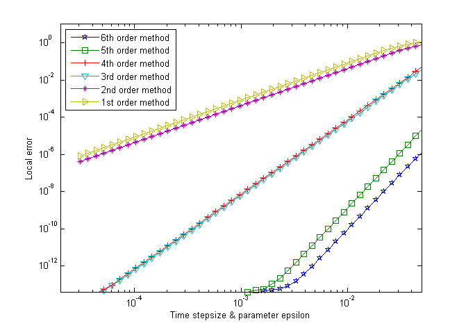
Refer to caption
Refer to caption
Refer to caption
Refer to caption
Figure 4: (t=ε)(t=\varepsilon)-dependence of the local error and of the deviation of the a posteriori error estimator. First row: As in Fig. 1, the plot on the left shows the empirical error of different splitting methods, while the plot on the right shows their observed orders. It is obvious that here the local order of the even order methods is reduced to 𝒪⁡(tp){\mathscr{O}}(t^{p}) while the odd order methods are not affected. Second row: Again, the plot on the left shows the empirical deviation of the a posteriori error estimator for different splitting methods and the plot on the right shows their observed orders. Compared to Fig. 1, the odd order methods suffer from an order reduction, while the even order methods show the expected dependence 𝒪⁡(tp+2){\mathscr{O}}(t^{p+2}). This advantage can be used to overcome the disadvantage observed in the first row (see (7.6)) even for less regular initial conditions. For all computations the initial condition was a shifted Gaussian at 2⋅1042\cdot 10^{4} gridpoints.

7.3 Defocussing laser beams and soliton solutions: Adaptive integration

For the following experiment we choose an application where a cubic Schrödinger equation without external potential arises, namely a model involving a self-defocussing laser beam in a nonlinear medium (see [27]).

The model describes the propagation of a weak intensity beam ψ⁡(x,y,z)\psi(x,y,z) in zz-direction via

i​ε​∂∂z​ψ​(x,y,z)=−12​ε2​(∂2∂x2+∂2∂y2)​ψ​(x,y,z)+ϑ​|ψ⁡(x,y,z)|2​ψ​(x,y,z),{\mathrm{i}}\mspace{1.5mu}\varepsilon\tfrac{\partial}{\partial z}\psi(x,y,z)=-\tfrac{1}{2}\mspace{1.5mu}\varepsilon^{2}\mspace{1.5mu}\big(\tfrac{\partial^{2}}{\partial x^{2}}+\tfrac{\partial^{2}}{\partial y^{2}}\big)\psi(x,y,z)+\vartheta|\psi(x,y,z)|^{2}\mspace{1.5mu}\psi(x,y,z)\mspace{1.5mu}, (7.7)

where ε\varepsilon describes the relationship between diffusion and focussing (arising from the nonlinear medium). For the special initial distribution ψ⁡(x,y,0)=tanh⁡(x)\psi(x,y,0)=\tanh(x) and ε=1\varepsilon=1, ϑ=1\vartheta=1, we obtain the solution

ψ⁡(x,y,z)=tanh⁡(x)​e−i​t​z.\psi(x,y,z)=\tanh(x)\mspace{1.5mu}{\mathrm{e}}^{-{\mathrm{i}}\mspace{1.5mu}t\mspace{1.5mu}z}\mspace{1.5mu}.

We have modified this and constructed a wave similar to a soliton by multiplying a Gaussian by tanh\tanh, which might be more stable under diffusion. For the results shown in Fig. 5 we have used the initial conditions

ψ1​(x,y,0)\displaystyle\psi_{1}(x,y,0) =A​exp⁡(−x2+y2r02)​tanh⁡(yys),\displaystyle=A\mspace{1.5mu}\exp\big(-\tfrac{x^{2}+y^{2}}{r_{0}^{2}}\big)\mspace{1.5mu}\tanh\big(\tfrac{y}{y_{s}}\big)\mspace{1.5mu},
ψ2​(x,y,0)\displaystyle\psi_{2}(x,y,0) =A​exp⁡(−x2+y2r02).\displaystyle=A\mspace{1.5mu}\exp\big(-\tfrac{x^{2}+y^{2}}{r_{0}^{2}}\big)\mspace{1.5mu}.

Numerical solutions have been obtained at 10001000 spatial gridpoints on the xx- and yy-axes and by a time-adaptive method of order four based on the a posteriori local error estimator (6.2) with a local absolute tolerance 10−810^{-8}. Comparing the two columns, we indeed see that the tanh\tanh profile provides a more stable signal than the Gaussian, which diffuses much faster and shows higher oscillations.

Refer to caption
Refer to caption
Refer to caption
Refer to caption
Refer to caption
Refer to caption
Figure 5: Defocussing laser beam with different shapes. Absolute value of beam intensity ψ\psi for problem (7.7) with ε=1100\varepsilon=\tfrac{1}{100}, Tend=5T_{\text{end}}=5 along the xx- and zz-axes for y=0y=0. In the first two rows we compare the absolute value (first row) and the real part (second row) of the solution. In the third row we display the adaptive stepsizes. Left column: Modulated Gaussian ψ1​(x,y,0)=exp⁡(−4​(x2+y2))​tanh⁡(x)\psi_{1}(x,y,0)=\exp(-4(x^{2}+y^{2}))\mspace{1.5mu}\tanh(x). Right column: Gaussian ψ2​(x,y,0)=exp⁡(−4​(x2+y2))\psi_{2}(x,y,0)=\exp(-4(x^{2}+y^{2})).

Appendix

Appendix A Technical tools

A.1 Gröbner-Alekseev formula (nonlinear variation of constant)

Proposition 2

Given a pair of initial value problems,

{z′​(t)=G⁡(t,z⁡(t))=F⁡(z⁡(t))+r⁡(t,z⁡(t)),0≤t≤Tz⁡(0)=u\displaystyle\begin{cases}\penalty\ z^{\prime}(t)=G(t,z(t))=F(z(t))+r(t,z(t))\mspace{1.5mu},\qquad 0\leq t\leq T\\ \penalty\ z(0)=u\end{cases} (A.1a)
{y′​(t)=F⁡(y⁡(t)), 0≤t≤Ty⁡(0)=u\displaystyle\begin{cases}\penalty\ y^{\prime}(t)=F(y(t))\mspace{1.5mu},\qquad\qquad\qquad\qquad\qquad\quad\penalty\ \penalty\ 0\leq t\leq T\\ \penalty\ y(0)=u\end{cases} (A.1b)

the solution z⁡(t)z(t) of (A.1a) can be expressed via the nonlinear variation of constant formula

z⁡(t)=ℰG​(t,u)=y⁡(t)+∫0t∂2ℰF​(t−τ,ℰG​(τ,u))​r​(τ,ℰG​(τ,u))​𝑑τ,0≤t≤T,z(t)=\mathcal{E}_{G}(t,u)=y(t)+\int_{0}^{t}\partial_{2}\mspace{1.5mu}\mathcal{E}_{F}(t-\tau,\mathcal{E}_{G}(\tau,u))\mspace{1.5mu}r(\tau,\mathcal{E}_{G}(\tau,u))\mspace{1.5mu}{\mathrm{d}}\tau,\quad 0\leq t\leq T\mspace{1.5mu}, (A.2)

where y​(t)=ℰF​(t,u)y(t)=\mathcal{E}_{F}(t,u) is the solution of (A.1b).

Proof

See [23] or [17].

A.2 L2L^{2} estimates for products of functions

For the following estimates we use Hölder’s inequality and Sobolev embeddings for estimating products in the L2L^{2}-norm, for spatial dimension d∈{1,2,3}d\in\{1,2,3\},

‖u​v‖L2\displaystyle\|u\mspace{1.5mu}v\|_{L^{2}} ≤‖u‖L4​‖v‖L4≤C​‖u‖H1​‖v‖H1,\displaystyle\leq\|u\|_{L^{4}}\mspace{1.5mu}\|v\|_{L^{4}}\leq C\mspace{1.5mu}\|u\|_{H^{1}}\mspace{1.5mu}\|v\|_{H^{1}}\mspace{1.5mu},
‖u​v‖L2\displaystyle\|u\mspace{1.5mu}v\|_{L^{2}} ≤C​‖u‖H2​‖v‖L2,\displaystyle\leq C\mspace{1.5mu}\|u\|_{H^{2}}\mspace{1.5mu}\|v\|_{L^{2}}\mspace{1.5mu},
‖u​v​w‖L2\displaystyle\|u\mspace{1.5mu}v\mspace{1.5mu}w\|_{L^{2}} ≤‖u‖L6​‖v‖L6​‖w‖L6≤C​‖u‖H1​‖v‖H1​‖w‖H1,\displaystyle\leq\|u\|_{L^{6}}\mspace{1.5mu}\|v\|_{L^{6}}\mspace{1.5mu}\|w\|_{L^{6}}\leq C\mspace{1.5mu}\|u\|_{H^{1}}\mspace{1.5mu}\|v\|_{H^{1}}\mspace{1.5mu}\|w\|_{H^{1}}\mspace{1.5mu},
‖u​v​w‖L2\displaystyle\|u\mspace{1.5mu}v\mspace{1.5mu}w\|_{L^{2}} ≤C​‖u​v‖H2​‖w‖L2,\displaystyle\leq C\mspace{1.5mu}\|u\mspace{1.5mu}v\|_{H^{2}}\mspace{1.5mu}\|w\|_{L^{2}}\mspace{1.5mu},
‖u​v​w​z‖L2\displaystyle\|u\mspace{1.5mu}v\mspace{1.5mu}w\mspace{1.5mu}z\|_{L^{2}} ≤C​‖u​v​w‖H2​‖z‖L2.\displaystyle\leq C\mspace{1.5mu}\|u\mspace{1.5mu}v\mspace{1.5mu}w\|_{H^{2}}\mspace{1.5mu}\|z\|_{L^{2}}\mspace{1.5mu}.

Since H2H^{2} forms an algebra, we can moreover estimate products in H2H^{2} as

‖u​v‖H2≤C​‖u‖H2​‖v‖H2.\|u\mspace{1.5mu}v\|_{H^{2}}\leq C\mspace{1.5mu}\|u\|_{H^{2}}\mspace{1.5mu}\|v\|_{H^{2}}\mspace{1.5mu}.

A.3 L2L^{2} estimates for mixed powers of xx and ∂ju\partial_{j}u

The following estimates are based on repeated integration by parts and the inequality of arithmetic and geometric means.

‖xj​∂ju‖L2\displaystyle\|x_{j}\mspace{1.5mu}\partial_{j}\mspace{1.5mu}u\|_{L^{2}} ≤C⁡(‖x2​u‖L2+‖u‖H2),\displaystyle\leq C\mspace{1.5mu}\big(\|x^{2}\mspace{1.5mu}u\|_{L^{2}}+\|u\|_{H^{2}}\big)\mspace{1.5mu},
‖xj2​∂ju‖L2\displaystyle\|x_{j}^{2}\mspace{1.5mu}\partial_{j}\mspace{1.5mu}u\|_{L^{2}} ≤C⁡(‖x4​u‖L2+‖x2​u‖L2+‖u‖H2),\displaystyle\leq C\mspace{1.5mu}\big(\|x^{4}\mspace{1.5mu}u\|_{L^{2}}+\|x^{2}\mspace{1.5mu}u\|_{L^{2}}+\|u\|_{H^{2}}\big)\mspace{1.5mu},
‖xj​∂j2u‖L2\displaystyle\|x_{j}\mspace{1.5mu}\partial_{j}^{2}\mspace{1.5mu}u\|_{L^{2}} ≤C⁡(‖x3​u‖L2+‖u‖H3),or‖xj​∂j2u‖L2≤C⁡(‖x3​u‖L2+‖u‖H3),\displaystyle\leq C\mspace{1.5mu}\big(\|x^{3}\mspace{1.5mu}u\|_{L^{2}}+\|u\|_{H^{3}}\big),\quad\text{or}\quad\|x_{j}\mspace{1.5mu}\partial_{j}^{2}\mspace{1.5mu}u\|_{L^{2}}\leq C\mspace{1.5mu}\big(\|x^{3}\mspace{1.5mu}u\|_{L^{2}}+\|u\|_{H^{3}}\big)\mspace{1.5mu},
‖xj2​∂j2u‖L2\displaystyle{\|x_{j}^{2}\mspace{1.5mu}\partial_{j}^{2}\mspace{1.5mu}u\|_{L^{2}}} ≤C⁡(‖x4​u‖L2+‖u‖H4).\displaystyle\leq C\mspace{1.5mu}\big(\|x^{4}\mspace{1.5mu}u\|_{L^{2}}+\|u\|_{H^{4}}\big)\mspace{1.5mu}.

Appendix B Derivation of integral representations for the first- and second-order defect terms

The integral representations (3.12) and (3.13) for the first- and second-order defect terms 𝒮(1)​(t,u)\mathcal{S}^{(1)}(t,u) and 𝒮(2)​(t,u)\mathcal{S}^{(2)}(t,u) are related to the analogous results for the general case, with AA and BB nonlinear, from [3], which were derived and verified with the help of computer algebra. Here we specialize for AA linear and give a rigorous proof, rearranging terms in a way which is appropriate for the present purpose, without explicating all technical details.

The idea is to evaluate the defect terms in a way containing no explicit time derivatives. This results in several subexpressions vanishing at t=0t=0 and satisfying certain linear evolution equations. Application of the variation of constant formulas

y′​(t)\displaystyle y^{\prime}(t) =12Ay(t)+r(t),y(0)=0⇒y(t)=∫0tℰA(12(t−τ))r(τ)dτ,\displaystyle=\tfrac{1}{2}\mspace{1.5mu}A\mspace{1.5mu}y(t)+r(t)\mspace{1.5mu},\penalty\ \penalty\ y(0)=0\quad\Rightarrow\quad y(t)=\int_{0}^{t}\mathcal{E}_{A}(\tfrac{1}{2}\mspace{1.5mu}(t-\tau))\mspace{1.5mu}r(\tau)\mspace{1.5mu}{\mathrm{d}}\tau\mspace{1.5mu}, (B.1a)
y′​(t)\displaystyle y^{\prime}(t) =B′(ℰB(t,u))y(t)+r(t),y(0)=0⇒y(t)=∫0t∂2ℰB(t−τ,ℰB(τ,u))r(τ)dτ.\displaystyle=B^{\prime}(\mathcal{E}_{B}(t,u))\mspace{1.5mu}y(t)+r(t),\mspace{1.5mu}\penalty\ \penalty\ y(0)=0\quad\Rightarrow\quad y(t)=\int_{0}^{t}\partial_{2}\mspace{1.5mu}\mathcal{E}_{B}(t-\tau,\mathcal{E}_{B}(\tau,u))\mspace{1.5mu}r(\tau)\mspace{1.5mu}{\mathrm{d}}\tau\mspace{1.5mu}. (B.1b)

then yields the desired integral forms.

To explain (B.1b) we note that

∂∂t​∂2ℰB​(t,u)​z=B′​(ℰB​(t,u))​∂2ℰB​(t,u)​z,(∂2ℰB​(t,u))−1=∂2ℰB​(−τ,ℰB​(τ,u)),∂2ℰB​(t,u)​∂2ℰB​(−τ,ℰB​(τ,u))=∂2ℰB​(t−τ,ℰB​(τ,u)).\displaystyle\begin{aligned} \tfrac{\partial}{\partial t}\partial_{2}\mathcal{E}_{B}(t,u)z&=B^{\prime}(\mathcal{E}_{B}(t,u))\mspace{1.5mu}\partial_{2}\mathcal{E}_{B}(t,u)z\mspace{1.5mu},\\ \big(\partial_{2}\mathcal{E}_{B}(t,u)\big)^{-1}&=\partial_{2}\mathcal{E}_{B}(-\tau,\mathcal{E}_{B}(\tau,u))\mspace{1.5mu},\\ \partial_{2}\mathcal{E}_{B}(t,u)\partial_{2}\mathcal{E}_{B}(-\tau,\mathcal{E}_{B}(\tau,u))&=\partial_{2}\mathcal{E}_{B}(t-\tau,\mathcal{E}_{B}(\tau,u))\mspace{1.5mu}.\end{aligned}

Hence by the linear variation of constant formula,

y⁡(t)\displaystyle y(t) =∂2ℰB​(t,u)​∫0t(∂2ℰB​(τ,u))−1​r​(τ)​𝑑τ=∫0t∂2ℰB​(t−τ,ℰB​(τ,u))​r​(τ)​𝑑τ.\displaystyle=\partial_{2}\mathcal{E}_{B}(t,u)\int_{0}^{t}\big(\partial_{2}\mathcal{E}_{B}(\tau,u)\big)^{-1}r(\tau)\mspace{1.5mu}{\mathrm{d}}\tau=\int_{0}^{t}\partial_{2}\mspace{1.5mu}\mathcal{E}_{B}(t-\tau,\mathcal{E}_{B}(\tau,u))\mspace{1.5mu}r(\tau)\mspace{1.5mu}{\mathrm{d}}\tau\mspace{1.5mu}.

B.1 The first-order defect 𝒮(1)​(t,u)\mathcal{S}^{(1)}(t,u)

The intermediate values of a Strang splitting step (3.2),

v\displaystyle v =v⁡(t,u)=ℰA​(12​t)​u,\displaystyle=v(t,u)=\mathcal{E}_{A}(\tfrac{1}{2}\mspace{1.5mu}t)\mspace{1.5mu}u\mspace{1.5mu}, (B.2a)
w\displaystyle w =w⁡(t,u)=ℰB​(t,v),\displaystyle=w(t,u)=\mathcal{E}_{B}(t,v)\mspace{1.5mu}, (B.2b)

(such that 𝒮⁡(t,u)=ℰA​(12​t,w)\mathcal{S}(t,u)=\mathcal{E}_{A}(\tfrac{1}{2}\mspace{1.5mu}t,w)) satisfy

∂∂t​v\displaystyle\tfrac{\partial}{\partial t}v =12​A​v,\displaystyle=\tfrac{1}{2}\mspace{1.5mu}A\mspace{1.5mu}v\mspace{1.5mu},
∂∂t​w\displaystyle\tfrac{\partial}{\partial t}w =B⁡(w)+∂2ℰB​(t,v)​∂∂t​v=B⁡(w)+12​∂2ℰB​(t,v)​A​v.\displaystyle=B(w)+\partial_{2}\mspace{1.5mu}\mathcal{E}_{B}(t,v)\mspace{1.5mu}\tfrac{\partial}{\partial t}v=B(w)+\tfrac{1}{2}\mspace{1.5mu}\partial_{2}\mspace{1.5mu}\mathcal{E}_{B}(t,v)\mspace{1.5mu}A\mspace{1.5mu}v\mspace{1.5mu}.

Thus,

∂∂t​𝒮​(t,u)\displaystyle\tfrac{\partial}{\partial t}\mathcal{S}(t,u) =∂∂t​(ℰA​(12​t)​w)\displaystyle=\tfrac{\partial}{\partial t}\big(\mathcal{E}_{A}(\tfrac{1}{2}\mspace{1.5mu}t)\mspace{1.5mu}w\big)
=12​A​𝒮​(t,u)+ℰA​(12​t,w)​∂∂t​w\displaystyle=\tfrac{1}{2}\mspace{1.5mu}A\mspace{1.5mu}\mathcal{S}(t,u)+\mathcal{E}_{A}(\tfrac{1}{2}\mspace{1.5mu}t,w)\mspace{1.5mu}\tfrac{\partial}{\partial t}w
=12​A​𝒮​(t,u)+ℰA​(12​t)​B​(w)+12​ℰA​(12​t)​∂2ℰB​(t,v)​A​v,\displaystyle=\tfrac{1}{2}\mspace{1.5mu}A\mspace{1.5mu}\mathcal{S}(t,u)+\mathcal{E}_{A}(\tfrac{1}{2}\mspace{1.5mu}t)\mspace{1.5mu}B(w)+\tfrac{1}{2}\mspace{1.5mu}\mathcal{E}_{A}(\tfrac{1}{2}\mspace{1.5mu}t)\mspace{1.5mu}\partial_{2}\mspace{1.5mu}\mathcal{E}_{B}(t,v)\mspace{1.5mu}A\mspace{1.5mu}v\mspace{1.5mu},

and for the defect 𝒮(1)\mathcal{S}^{(1)} this gives

𝒮(1)​(t,u)\displaystyle\mathcal{S}^{(1)}(t,u) =∂∂t​𝒮​(t,u)−A​𝒮​(t,u)−B⁡(𝒮⁡(t,u))\displaystyle=\tfrac{\partial}{\partial t}\mathcal{S}(t,u)-A\mspace{1.5mu}\mathcal{S}(t,u)-B(\mathcal{S}(t,u))
=ℰA​(12​t)​B​(w)+12​ℰA​(12​t)​∂2ℰB​(t,v)​A​v−12​A​𝒮​(t,u)−B⁡(𝒮⁡(t,u))\displaystyle=\mathcal{E}_{A}(\tfrac{1}{2}\mspace{1.5mu}t)\mspace{1.5mu}B(w)+\tfrac{1}{2}\mspace{1.5mu}\mathcal{E}_{A}(\tfrac{1}{2}\mspace{1.5mu}t)\mspace{1.5mu}\partial_{2}\mspace{1.5mu}\mathcal{E}_{B}(t,v)\mspace{1.5mu}A\mspace{1.5mu}v-\tfrac{1}{2}\mspace{1.5mu}A\mspace{1.5mu}\mathcal{S}(t,u)-B(\mathcal{S}(t,u))
=ℰA​(12​t)​B​(w)+12​ℰA​(12​t)​∂2ℰB​(t,v)​A​v−12​A​ℰA​(12​t)​w−B⁡(ℰA​(12​t)​w)\displaystyle=\mathcal{E}_{A}(\tfrac{1}{2}\mspace{1.5mu}t)\mspace{1.5mu}B(w)+\tfrac{1}{2}\mspace{1.5mu}\mathcal{E}_{A}(\tfrac{1}{2}\mspace{1.5mu}t)\mspace{1.5mu}\partial_{2}\mspace{1.5mu}\mathcal{E}_{B}(t,v)\mspace{1.5mu}A\mspace{1.5mu}v-\tfrac{1}{2}\mspace{1.5mu}A\mspace{1.5mu}\mathcal{E}_{A}(\tfrac{1}{2}\mspace{1.5mu}t)\mspace{1.5mu}w-B(\mathcal{E}_{A}(\tfrac{1}{2}\mspace{1.5mu}t)\mspace{1.5mu}w)
=ℰA​(12​t)​B​(w)+12​ℰA​(12​t)​∂2ℰB​(t,v)​A​v−12​ℰA​(12​t)​A​w−B⁡(ℰA​(12​t)​w),\displaystyle=\mathcal{E}_{A}(\tfrac{1}{2}\mspace{1.5mu}t)\mspace{1.5mu}B(w)+\tfrac{1}{2}\mspace{1.5mu}\mathcal{E}_{A}(\tfrac{1}{2}\mspace{1.5mu}t)\mspace{1.5mu}\partial_{2}\mspace{1.5mu}\mathcal{E}_{B}(t,v)\mspace{1.5mu}A\mspace{1.5mu}v-\tfrac{1}{2}\mspace{1.5mu}\mathcal{E}_{A}(\tfrac{1}{2}\mspace{1.5mu}t)\mspace{1.5mu}A\mspace{1.5mu}w-B(\mathcal{E}_{A}(\tfrac{1}{2}\mspace{1.5mu}t)\mspace{1.5mu}w)\mspace{1.5mu},

which can be written in the form

𝒮(1)​(t,u)\displaystyle\mathcal{S}^{(1)}(t,u) =ℰA​(12​t)​B​(w)−B⁡(ℰA​(12​t)​w)\displaystyle=\mathcal{E}_{A}(\tfrac{1}{2}\mspace{1.5mu}t)\mspace{1.5mu}B(w)-B(\mathcal{E}_{A}(\tfrac{1}{2}\mspace{1.5mu}t)\mspace{1.5mu}w) (B.3a)
+12​ℰA​(12​t)​(∂2ℰB​(t,v)​A​v−A​ℰB​(t,v)).\displaystyle\quad{}+\tfrac{1}{2}\mspace{1.5mu}\mathcal{E}_{A}(\tfrac{1}{2}\mspace{1.5mu}t)\big(\partial_{2}\mspace{1.5mu}\mathcal{E}_{B}(t,v)\mspace{1.5mu}A\mspace{1.5mu}v-A\mspace{1.5mu}\mathcal{E}_{B}(t,v)\big)\mspace{1.5mu}. (B.3b)

In order to find an integral representation for 𝒮(1)​(t,u)\mathcal{S}^{(1)}(t,u), we separately consider the terms (B.3a) and (B.3b), with vv and ww fixed. Differentiating with respect to tt we find that they satisfy the following evolution equations.

(B.3a):

𝒮(a)(1)​(t)=ℰA​(12​t)​B​(w)−B⁡(ℰA​(12​t)​w)\mathcal{S}^{(1)}_{(a)}(t)=\mathcal{E}_{A}(\tfrac{1}{2}\mspace{1.5mu}t)\mspace{1.5mu}B(w)-B(\mathcal{E}_{A}(\tfrac{1}{2}\mspace{1.5mu}t)\mspace{1.5mu}w) satisfies 𝒮(a)(1)​(0)=0\mathcal{S}^{(1)}_{(a)}(0)=0, and

∂∂t​𝒮(a)(1)​(t)=12​A​𝒮(a)(1)​(t)+12​[A,B]​(ℰA​(12​t)​w).\tfrac{\partial}{\partial t}\mathcal{S}^{(1)}_{(a)}(t)=\tfrac{1}{2}\mspace{1.5mu}A\mspace{1.5mu}\mathcal{S}^{(1)}_{(a)}(t)+\tfrac{1}{2}[A,B](\mathcal{E}_{A}(\tfrac{1}{2}\mspace{1.5mu}t)\mspace{1.5mu}w)\mspace{1.5mu}. (B.4a)

In (B.3b), we consider the expression within (…)\big(\ldots\big):

(B.3b):

𝒮(b)(1)​(t)=∂2ℰB​(t,v)​A​v−A​ℰB​(t,v)\mathcal{S}^{(1)}_{(b)}(t)=\partial_{2}\mspace{1.5mu}\mathcal{E}_{B}(t,v)\mspace{1.5mu}A\mspace{1.5mu}v-A\mspace{1.5mu}\mathcal{E}_{B}(t,v) satisfies 𝒮(b)(1)​(0)=0\mathcal{S}^{(1)}_{(b)}(0)=0, and

∂∂t​𝒮(b)(1)​(t)=B′​(ℰB​(t,v))​𝒮(b)(1)​(t,v)+[B,A]​(ℰB​(t,v)).\tfrac{\partial}{\partial t}\mathcal{S}^{(1)}_{(b)}(t)=B^{\prime}(\mathcal{E}_{B}(t,v))\mspace{1.5mu}\mathcal{S}^{(1)}_{(b)}(t,v)+[B,A](\mathcal{E}_{B}(t,v))\mspace{1.5mu}. (B.4b)

Finally, applying (B.1a) and (B.1b), recombination and substituting v=ℰA​(12​t)​uv=\mathcal{E}_{A}(\frac{1}{2}t)\mspace{1.5mu}u, w=ℰB​(t,ℰA​(12​t)​u)w=\mathcal{E}_{B}(t,\mathcal{E}_{A}(\frac{1}{2}t)\mspace{1.5mu}u) leads to the integral representation (3.12) for 𝒮(1)​(t,u)\mathcal{S}^{(1)}(t,u).

B.2 The second-order defect 𝒮(2)​(t,u)\mathcal{S}^{(2)}(t,u)

To evaluate 𝒮(2)\mathcal{S}^{(2)} defined in (3.8b), we proceed in an analogous way as for 𝒮(1)\mathcal{S}^{(1)}, with vv, ww defined in (B.2).
We start by differentiating the expression for 𝒮(1)\mathcal{S}^{(1)} from (3.6) with respect to tt,

∂∂t​𝒮(1)​(t,u)\displaystyle\tfrac{\partial}{\partial t}\mathcal{S}^{(1)}(t,u) =(A+B′​(𝒮⁡(t,u)))​𝒮(1)​(t,u)\displaystyle=\big(A+B^{\prime}(\mathcal{S}(t,u))\big)\mspace{1.5mu}\mathcal{S}^{(1)}(t,u)
−B′(ℰA(12t)w)ℰA(12t)∂2ℰB(t,v)Av+ℰA(12t)B′(w)∂2ℰB(t,v)Av\displaystyle\quad{}-B^{\prime}(\mathcal{E}_{A}(\tfrac{1}{2}\mspace{1.5mu}t)\mspace{1.5mu}w)\mspace{1.5mu}\mathcal{E}_{A}(\tfrac{1}{2}\mspace{1.5mu}t)\mspace{1.5mu}\partial_{2}\mspace{1.5mu}\mathcal{E}_{B}(t,v)\mspace{1.5mu}A\mspace{1.5mu}v+\mathcal{E}_{A}(\tfrac{1}{2}\mspace{1.5mu}t)\mspace{1.5mu}B^{\prime}(w)\mspace{1.5mu}\partial_{2}\mspace{1.5mu}\mathcal{E}_{B}(t,v)\mspace{1.5mu}A\mspace{1.5mu}v
−A​ℰA​(12​t)​B​(w)+A​B​(ℰA​(12​t)​w)−12​A​ℰA​(12​t)​∂2ℰB​(t,v)​A​v\displaystyle\quad{}-A\mspace{1.5mu}\mathcal{E}_{A}(\tfrac{1}{2}\mspace{1.5mu}t)\mspace{1.5mu}B(w)+A\mspace{1.5mu}B(\mathcal{E}_{A}(\tfrac{1}{2}\mspace{1.5mu}t)\mspace{1.5mu}w)-\tfrac{1}{2}\mspace{1.5mu}A\mspace{1.5mu}\mathcal{E}_{A}(\tfrac{1}{2}\mspace{1.5mu}t)\mspace{1.5mu}\partial_{2}\mspace{1.5mu}\mathcal{E}_{B}(t,v)\mspace{1.5mu}A\mspace{1.5mu}v
+14ℰA(12t)∂2ℰB(t,v)A2v+14A2ℰA(12t)w\displaystyle\quad{}+\tfrac{1}{4}\mspace{1.5mu}\mathcal{E}_{A}(\tfrac{1}{2}\mspace{1.5mu}t)\mspace{1.5mu}\partial_{2}\mspace{1.5mu}\mathcal{E}_{B}(t,v)\mspace{1.5mu}A^{2}\mspace{1.5mu}v+\tfrac{1}{4}\mspace{1.5mu}A^{2}\mspace{1.5mu}\mathcal{E}_{A}(\tfrac{1}{2}\mspace{1.5mu}t)\mspace{1.5mu}w
+14ℰA(12t)∂22ℰB(t,v)(Av,Av)+ℰA(12t)B′(w)B(w)\displaystyle\quad{}+\tfrac{1}{4}\mspace{1.5mu}\mathcal{E}_{A}(\tfrac{1}{2}\mspace{1.5mu}t)\mspace{1.5mu}\partial_{2}^{2}\mspace{1.5mu}\mathcal{E}_{B}(t,v)(A\mspace{1.5mu}v,A\mspace{1.5mu}v)+\mathcal{E}_{A}(\tfrac{1}{2}\mspace{1.5mu}t)\mspace{1.5mu}B^{\prime}(w)\mspace{1.5mu}B(w)
+B′​(ℰA​(12​t)​w)​B​(ℰA​(12​t)​w)−2​B′​(ℰA​(12​t)​w)​ℰA​(12​t)​B​(w).\displaystyle\quad{}+B^{\prime}(\mathcal{E}_{A}(\tfrac{1}{2}\mspace{1.5mu}t)\mspace{1.5mu}w)\mspace{1.5mu}B(\mathcal{E}_{A}(\tfrac{1}{2}\mspace{1.5mu}t)\mspace{1.5mu}w)-2\mspace{1.5mu}B^{\prime}(\mathcal{E}_{A}(\tfrac{1}{2}\mspace{1.5mu}t)\mspace{1.5mu}w)\mspace{1.5mu}\mathcal{E}_{A}(\tfrac{1}{2}\mspace{1.5mu}t)\mspace{1.5mu}B(w)\mspace{1.5mu}.

Subtracting F′​(𝒮⁡(t,u))​𝒮(1)​(t,u)=(A+B′​(𝒮⁡(t,u)))​𝒮(1)​(t,u)F^{\prime}(\mathcal{S}(t,u))\mspace{1.5mu}\mathcal{S}^{(1)}(t,u)=(A+B^{\prime}(\mathcal{S}(t,u)))\mspace{1.5mu}\mathcal{S}^{(1)}(t,u) and rearranging terms yields

𝒮(2)​(t,u)\displaystyle\mathcal{S}^{(2)}(t,u) =(ℰA​(12​t)​B′​(w)−B′​(ℰA​(12​t)​w)​ℰA​(12​t))​∂2ℰB​(t,v)​A​v\displaystyle=\big(\mathcal{E}_{A}(\tfrac{1}{2}\mspace{1.5mu}t)\mspace{1.5mu}B^{\prime}(w)-B^{\prime}(\mathcal{E}_{A}(\tfrac{1}{2}\mspace{1.5mu}t)\mspace{1.5mu}w)\mspace{1.5mu}\mathcal{E}_{A}(\tfrac{1}{2}\mspace{1.5mu}t)\big)\mspace{1.5mu}\partial_{2}\mspace{1.5mu}\mathcal{E}_{B}(t,v)\mspace{1.5mu}A\mspace{1.5mu}v (B.5a)
+(A+B′​(ℰA​(12​t)​w))​(B⁡(ℰA​(12​t)​w)−ℰA​(12​t)​B​(w))\displaystyle\quad{}+\big(A+B^{\prime}(\mathcal{E}_{A}(\tfrac{1}{2}\mspace{1.5mu}t)\mspace{1.5mu}w)\big)\mspace{1.5mu}\big(B(\mathcal{E}_{A}(\tfrac{1}{2}t)\mspace{1.5mu}w)-\mathcal{E}_{A}(\tfrac{1}{2}t)\mspace{1.5mu}B(w)\big) (B.5b)
+(ℰA​(12​t)​B′​(w)−B′​(ℰA​(12​t)​w)​ℰA​(12​t))​B​(w)\displaystyle\quad{}+\big(\mathcal{E}_{A}(\tfrac{1}{2}\mspace{1.5mu}t)\mspace{1.5mu}B^{\prime}(w)-B^{\prime}(\mathcal{E}_{A}(\tfrac{1}{2}\mspace{1.5mu}t)\mspace{1.5mu}w)\mspace{1.5mu}\mathcal{E}_{A}(\tfrac{1}{2}\mspace{1.5mu}t)\big)\mspace{1.5mu}B(w) (B.5c)
+14​ℰA​(12​t)​(A⁡(A​ℰB​(t,v)−∂2ℰB​(t,v)​A​v)CLOSE\displaystyle\quad{}+\tfrac{1}{4}\mspace{1.5mu}\mathcal{E}_{A}(\tfrac{1}{2}\mspace{1.5mu}t)\Big(A\big(A\mspace{1.5mu}\mathcal{E}_{B}(t,v)-\partial_{2}\mspace{1.5mu}\mathcal{E}_{B}(t,v)\mspace{1.5mu}A\mspace{1.5mu}v\big) (B.5d)
−(A​∂2ℰB​(t,v)−∂2ℰB​(t,v)​A)​A​v\displaystyle\qquad\qquad\qquad\quad{}-\big(A\mspace{1.5mu}\partial_{2}\mspace{1.5mu}\mathcal{E}_{B}(t,v)-\partial_{2}\mspace{1.5mu}\mathcal{E}_{B}(t,v)\mspace{1.5mu}A\big)\mspace{1.5mu}A\mspace{1.5mu}v (B.5e)
+∂22ℰB(t,v)(Av,Av)).\displaystyle\qquad\qquad\qquad\quad{}+\partial_{2}^{2}\mspace{1.5mu}\mathcal{E}_{B}(t,v)(A\mspace{1.5mu}v,A\mspace{1.5mu}v)\Big)\mspace{1.5mu}. (B.5f)

Evaluation of 𝒮(2)​(t,u)\mathcal{S}^{(2)}(t,u) at t=0t=0 shows 𝒮(2)​(0,u)=0\mathcal{S}^{(2)}(0,u)=0, hence 𝒮(2)​(t,u)=𝒪⁡(t)\mathcal{S}^{(2)}(t,u)={\mathscr{O}}(t).

In order to find an integral representation for 𝒮(2)​(t,u)\mathcal{S}^{(2)}(t,u), we separately consider the terms (B.5a)–(B.5f), with vv, ww and z:=∂2ℰB​(t,v)​A​vz:=\partial_{2}\mspace{1.5mu}\mathcal{E}_{B}(t,v)\mspace{1.5mu}A\mspace{1.5mu}v fixed. Differentiating with respect to tt we find that they satisfy the following linear evolution equations.

(B.5a):

𝒮(a)(2)​(t)=(ℰA​(12​t)​B′​(w)−B′​(ℰA​(12​t)​w)​ℰA​(12​t))​z\mathcal{S}^{(2)}_{(a)}(t)=\big(\mathcal{E}_{A}(\tfrac{1}{2}\mspace{1.5mu}t)\mspace{1.5mu}B^{\prime}(w)-B^{\prime}(\mathcal{E}_{A}(\tfrac{1}{2}\mspace{1.5mu}t)\mspace{1.5mu}w)\mspace{1.5mu}\mathcal{E}_{A}(\tfrac{1}{2}t)\big)z satisfies 𝒮(a)(2)​(0)=0\mathcal{S}^{(2)}_{(a)}(0)=0, and

∂∂t​𝒮(a)(2)​(t)\displaystyle\tfrac{\partial}{\partial t}\mathcal{S}^{(2)}_{(a)}(t) =12​A​𝒮(a)(2)​(t)\displaystyle=\tfrac{1}{2}\mspace{1.5mu}A\mspace{1.5mu}\mathcal{S}^{(2)}_{(a)}(t) (B.6a)
+12​[A,B′​(ℰA​(12​t)​w)]​A​ℰA​(12​t)​w+12​[A,B′​(ℰA​(12​t)​w)]​ℰA​(12​t)​(z−A​w)\displaystyle\quad{}+\tfrac{1}{2}\mspace{1.5mu}[A,B^{\prime}(\mathcal{E}_{A}(\tfrac{1}{2}\mspace{1.5mu}t)\mspace{1.5mu}w)]A\mspace{1.5mu}\mathcal{E}_{A}(\tfrac{1}{2}\mspace{1.5mu}t)w+\tfrac{1}{2}\mspace{1.5mu}[A,B^{\prime}(\mathcal{E}_{A}(\tfrac{1}{2}\mspace{1.5mu}t)\mspace{1.5mu}w)]\mspace{1.5mu}\mathcal{E}_{A}(\tfrac{1}{2}\mspace{1.5mu}t)\mspace{1.5mu}\big(z-A\mspace{1.5mu}w\big)
−12​B′′​(ℰA​(12​t)​w)​(A​ℰA​(12​t)​w,ℰA​(12​t)​(z−A​w+A​w)).\displaystyle\quad{}-\tfrac{1}{2}\mspace{1.5mu}B^{\prime\prime}(\mathcal{E}_{A}(\tfrac{1}{2}\mspace{1.5mu}t)\mspace{1.5mu}w)\mspace{1.5mu}\big(A\mspace{1.5mu}\mathcal{E}_{A}(\tfrac{1}{2}\mspace{1.5mu}t)\mspace{1.5mu}w,\mathcal{E}_{A}(\tfrac{1}{2}\mspace{1.5mu}t)\mspace{1.5mu}(z-A\mspace{1.5mu}w+A\mspace{1.5mu}w)\big)\mspace{1.5mu}.
(B.5b):

𝒮(b)(2)​(t)=(A+B′​(ℰA​(12​t)​w))​(B⁡(ℰA​(12​t)​w)−ℰA​(12​t)​B​(w))\mathcal{S}^{(2)}_{(b)}(t)=\big(A+B^{\prime}(\mathcal{E}_{A}(\tfrac{1}{2}\mspace{1.5mu}t)\mspace{1.5mu}w)\big)\mspace{1.5mu}\big(B(\mathcal{E}_{A}(\tfrac{1}{2}t)\mspace{1.5mu}w)-\mathcal{E}_{A}(\tfrac{1}{2}t)\mspace{1.5mu}B(w)\big) satisfies 𝒮(b)(2)​(0)=0\mathcal{S}^{(2)}_{(b)}(0)=0, and

∂∂t​𝒮(b)(2)​(t)\displaystyle\tfrac{\partial}{\partial t}\mathcal{S}^{(2)}_{(b)}(t) =12​A​𝒮(b)(2)​(t)\displaystyle=\tfrac{1}{2}\mspace{1.5mu}A\mspace{1.5mu}\mathcal{S}^{(2)}_{(b)}(t) (B.6b)
+12​A​[B,A]​ℰA​(12​t)​w+12​B′​(ℰA​(12​t)​w)​[B,A]​ℰA​(12​t)​w\displaystyle\quad{}+\tfrac{1}{2}\mspace{1.5mu}A\mspace{1.5mu}[B\mspace{1.5mu},A]\mspace{1.5mu}\mathcal{E}_{A}(\tfrac{1}{2}\mspace{1.5mu}t)\mspace{1.5mu}w+\tfrac{1}{2}\mspace{1.5mu}B^{\prime}(\mathcal{E}_{A}(\tfrac{1}{2}\mspace{1.5mu}t)\mspace{1.5mu}w)\mspace{1.5mu}[B\mspace{1.5mu},A]\mspace{1.5mu}\mathcal{E}_{A}(\tfrac{1}{2}\mspace{1.5mu}t)\mspace{1.5mu}w
−12​B′′​(ℰA​(12​t)​w)​(A​ℰA​(12​t)​w,ℰA​(12​t)​B​(w)−B⁡(ℰA​(12​t)​w))\displaystyle\quad{}-\tfrac{1}{2}\mspace{1.5mu}B^{\prime\prime}(\mathcal{E}_{A}(\tfrac{1}{2}\mspace{1.5mu}t)\mspace{1.5mu}w)\big(A\mspace{1.5mu}\mathcal{E}_{A}(\tfrac{1}{2}\mspace{1.5mu}t)\mspace{1.5mu}w,\mathcal{E}_{A}(\tfrac{1}{2}\mspace{1.5mu}t)\mspace{1.5mu}B(w)-B(\mathcal{E}_{A}(\tfrac{1}{2}\mspace{1.5mu}t)\mspace{1.5mu}w)\big)
+12​[A,B′​(ℰA​(12​t)​w)]​(ℰA​(12​t)​B​(w)−B⁡(ℰA​(12​t)​w)).\displaystyle\quad{}+\tfrac{1}{2}\mspace{1.5mu}[A,B^{\prime}(\mathcal{E}_{A}(\tfrac{1}{2}\mspace{1.5mu}t)\mspace{1.5mu}w)]\mspace{1.5mu}\big(\mathcal{E}_{A}(\tfrac{1}{2}\mspace{1.5mu}t)\mspace{1.5mu}B(w)-B(\mathcal{E}_{A}(\tfrac{1}{2}\mspace{1.5mu}t)\mspace{1.5mu}w)\big)\mspace{1.5mu}.
(B.5c):

𝒮(c)(2)​(t)=(ℰA​(12​t)​B′​(w)−B′​(ℰA​(12​t)​w)​ℰA​(12​t))​B​(w)\mathcal{S}^{(2)}_{(c)}(t)=\big(\mathcal{E}_{A}(\tfrac{1}{2}\mspace{1.5mu}t)\mspace{1.5mu}B^{\prime}(w)-B^{\prime}(\mathcal{E}_{A}(\tfrac{1}{2}\mspace{1.5mu}t)\mspace{1.5mu}w)\mspace{1.5mu}\mathcal{E}_{A}(\tfrac{1}{2}t)\big)\mspace{1.5mu}B(w), satisfies 𝒮(c)(2)​(0)=0\mathcal{S}^{(2)}_{(c)}(0)=0, and

∂∂t​𝒮(c)(2)​(t)\displaystyle\tfrac{\partial}{\partial t}\mathcal{S}^{(2)}_{(c)}(t) =12​A​𝒮(c)(2)​(t)+12​[A,B′​(ℰA​(12​t)​w)]​ℰA​(12​t)​B​(w)\displaystyle=\tfrac{1}{2}\mspace{1.5mu}A\mspace{1.5mu}\mathcal{S}^{(2)}_{(c)}(t)+\tfrac{1}{2}\mspace{1.5mu}[A,B^{\prime}(\mathcal{E}_{A}(\tfrac{1}{2}\mspace{1.5mu}t)\mspace{1.5mu}w)]\mspace{1.5mu}\mathcal{E}_{A}(\tfrac{1}{2}\mspace{1.5mu}t)\mspace{1.5mu}B(w) (B.6c)
−12​B′′​(ℰA​(12​t)​w)​(A​ℰA​(12​t)​w,ℰA​(12​t)​B​(w)).\displaystyle\qquad\qquad\qquad{}-\tfrac{1}{2}\mspace{1.5mu}B^{\prime\prime}(\mathcal{E}_{A}(\tfrac{1}{2}\mspace{1.5mu}t)\mspace{1.5mu}w)\big(A\mspace{1.5mu}\mathcal{E}_{A}(\tfrac{1}{2}\mspace{1.5mu}t)\mspace{1.5mu}w,\mathcal{E}_{A}(\tfrac{1}{2}\mspace{1.5mu}t)\mspace{1.5mu}B(w)\big)\mspace{1.5mu}.

In (B.5d)–(B.5f), we consider the expressions within (…)\big(\ldots\big):

(B.5d):

𝒮(d)(2)​(t)=A⁡(A​ℰB​(t,v)−∂2ℰB​(t,v)​A​v)\mathcal{S}^{(2)}_{(d)}(t)=A\big(A\mspace{1.5mu}\mathcal{E}_{B}(t,v)-\partial_{2}\mspace{1.5mu}\mathcal{E}_{B}(t,v)\mspace{1.5mu}A\mspace{1.5mu}v\big) satisfies 𝒮(d)(2)​(0)=0\mathcal{S}^{(2)}_{(d)}(0)=0, and

∂∂t​𝒮(d)(2)​(t)\displaystyle\tfrac{\partial}{\partial t}\mathcal{S}^{(2)}_{(d)}(t) =B′​(ℰB​(t,v))​(𝒮(d)(2)​(t))\displaystyle=B^{\prime}(\mathcal{E}_{B}(t,v))\big(\mathcal{S}^{(2)}_{(d)}(t)\big) (B.6d)
+[A,[A,B]]​(ℰB​(t,v))\displaystyle\quad{}+[A,[A,B]](\mathcal{E}_{B}(t,v))
+2​[A,B′​(ℰB​(t,v))]​A​ℰB​(t,v)−[A,B′​(ℰB​(t,v))]​∂2ℰB​(t,v)​A​v\displaystyle\quad{}+2\mspace{1.5mu}[A,B^{\prime}(\mathcal{E}_{B}(t,v))]\mspace{1.5mu}A\mspace{1.5mu}\mathcal{E}_{B}(t,v)-[A,B^{\prime}(\mathcal{E}_{B}(t,v))]\mspace{1.5mu}\partial_{2}\mspace{1.5mu}\mathcal{E}_{B}(t,v)\mspace{1.5mu}A\mspace{1.5mu}v
−B′′​(ℰB​(t,v))​(A​ℰB​(t,v),A​ℰB​(t,v)).\displaystyle\quad{}-B^{\prime\prime}(\mathcal{E}_{B}(t,v))\big(A\mspace{1.5mu}\mathcal{E}_{B}(t,v),A\mspace{1.5mu}\mathcal{E}_{B}(t,v)\big)\mspace{1.5mu}.
(B.5e):

𝒮(e)(2)​(t)=(A​∂2ℰB​(t,v)−∂2ℰB​(t,v)​A)​A​v\mathcal{S}^{(2)}_{(e)}(t)=\big(A\mspace{1.5mu}\partial_{2}\mspace{1.5mu}\mathcal{E}_{B}(t,v)-\partial_{2}\mspace{1.5mu}\mathcal{E}_{B}(t,v)\mspace{1.5mu}A\big)\mspace{1.5mu}A\mspace{1.5mu}v satisfies 𝒮(e)(2)​(0)=0\mathcal{S}^{(2)}_{(e)}(0)=0, and

∂∂t​𝒮(e)(2)​(t)=B′​(ℰB​(t,v))​(𝒮(e)(2)​(t))+[A,B′​(ℰB​(t,v))]​∂2ℰB​(t,v)​A​v.\tfrac{\partial}{\partial t}\mathcal{S}^{(2)}_{(e)}(t)=B^{\prime}(\mathcal{E}_{B}(t,v))\big(\mathcal{S}^{(2)}_{(e)}(t)\big)+[A,B^{\prime}(\mathcal{E}_{B}(t,v))]\mspace{1.5mu}\partial_{2}\mspace{1.5mu}\mathcal{E}_{B}(t,v)\mspace{1.5mu}A\mspace{1.5mu}v\mspace{1.5mu}. (B.6e)
(B.5f):

𝒮(f)(2)​(t)=∂22ℰB​(t,v)​(A​v,A​v)\mathcal{S}^{(2)}_{(f)}(t)=\partial_{2}^{2}\mspace{1.5mu}\mathcal{E}_{B}(t,v)(A\mspace{1.5mu}v,A\mspace{1.5mu}v) satisfies 𝒮(f)(2)​(0)=0\mathcal{S}^{(2)}_{(f)}(0)=0, and

∂∂t​𝒮(f)(2)​(t)=B′​(ℰB​(t,v))​(𝒮(f)(2)​(t))+B′′​(ℰB​(t,v))​(∂2ℰB​(t,v)​A​v,∂2ℰB​(t,v)​A​v).\tfrac{\partial}{\partial t}\mathcal{S}^{(2)}_{(f)}(t)=B^{\prime}(\mathcal{E}_{B}(t,v))\big(\mathcal{S}^{(2)}_{(f)}(t)\big)+B^{\prime\prime}(\mathcal{E}_{B}(t,v))\big(\partial_{2}\mspace{1.5mu}\mathcal{E}_{B}(t,v)\mspace{1.5mu}A\mspace{1.5mu}v,\partial_{2}\mspace{1.5mu}\mathcal{E}_{B}(t,v)\mspace{1.5mu}A\mspace{1.5mu}v\big)\mspace{1.5mu}. (B.6f)

Finally, applying (B.1a) and (B.1b), respectively, recombination and substituting v=ℰA​(12​t)​uv=\mathcal{E}_{A}(\frac{1}{2}t)\mspace{1.5mu}u, w=ℰB​(t,ℰA​(12​t)​u)w=\mathcal{E}_{B}(t,\mathcal{E}_{A}(\frac{1}{2}t)\mspace{1.5mu}u) and z=∂2ℰB​(t,v)​A​vz=\partial_{2}\mspace{1.5mu}\mathcal{E}_{B}(t,v)\mspace{1.5mu}A\mspace{1.5mu}v leads to the integral representation (3.13) for 𝒮(2)​(t,u)\mathcal{S}^{(2)}(t,u).

Appendix C Auxiliary estimates for the NLS case

C.1 Estimate of ‖∂2ℰF​(τ1−τ2,𝒮⁡(τ2,u))⋅𝒮(2)​(τ2,u)‖L2\big\|\partial_{2}\mspace{1.5mu}\mathcal{E}_{F}(\tau_{1}-\tau_{2},\mathcal{S}(\tau_{2},u))\cdot\mathcal{S}^{(2)}(\tau_{2},u)\big\|_{L^{2}}

For a detailed study of the estimate (5.1b), we need to estimate the arising expressions in ℒ(2)​(t,u){\mathcal{L}}^{(2)}(t,u) as

∥∂2ℰF(t−τ2,𝒮(τ2,u))𝒮(2)(τ2,u)∥L2≤C1+C2⋅∥𝒮(2)(τ2,u)∥L2≤C1+C2⋅τ2sup0≤τ3≤τ2∥𝒔(2)(τ2,τ3,u)∥L2,\|\partial_{2}\mspace{1.5mu}\mathcal{E}_{F}(t-\tau_{2},\mathcal{S}(\tau_{2},u))\mathcal{S}^{(2)}(\tau_{2},u)\|_{L^{2}}\leq C_{1}+C_{2}\cdot\|\mathcal{S}^{(2)}(\tau_{2},u)\|_{L^{2}}\leq C_{1}+C_{2}\cdot\tau_{2}\mspace{1.5mu}\sup_{0\leq\tau_{3}\leq\tau_{2}}\|\bm{s}^{(2)}(\tau_{2},\tau_{3},u)\|_{L^{2}}\mspace{1.5mu},

with constants C1,C2C_{1},\mspace{1.5mu}C_{2} resulting from Gronwall estimates.

We substitute

g=𝒮(2)​(τ2,u),w=𝒮⁡(τ2,u)\displaystyle g=\mathcal{S}^{(2)}(\tau_{2},u)\mspace{1.5mu},\quad w=\mathcal{S}(\tau_{2},u)

and apply the linear variation of constant formula in the following way,

∂∂t​∂2ℰF​(t−τ2,w)​g\displaystyle\tfrac{\partial}{\partial t}\partial_{2}\mspace{1.5mu}\mathcal{E}_{F}(t-\tau_{2},w)\mspace{1.5mu}g =F′​(ℰF​(t−τ2,w))​∂2ℰF​(t−τ2,w)​g\displaystyle=F^{\prime}(\mathcal{E}_{F}(t-\tau_{2},w))\partial_{2}\mspace{1.5mu}\mathcal{E}_{F}(t-\tau_{2},w)\mspace{1.5mu}g
=A​∂2ℰF​(t−τ2,w)​g+B′​(ℰF​(t−τ2,w))​∂2ℰF​(t−τ2,w)​g,\displaystyle=A\mspace{1.5mu}\partial_{2}\mspace{1.5mu}\mathcal{E}_{F}(t-\tau_{2},w)\mspace{1.5mu}g+B^{\prime}(\mathcal{E}_{F}(t-\tau_{2},w))\mspace{1.5mu}\partial_{2}\mspace{1.5mu}\mathcal{E}_{F}(t-\tau_{2},w)g\mspace{1.5mu},
∂2ℰF​(t−τ2,w)|t=τ2​g\displaystyle\partial_{2}\mspace{1.5mu}\mathcal{E}_{F}(t-\tau_{2},w)\mspace{1.5mu}\Big|_{t=\tau_{2}}g =g,\displaystyle=g\mspace{1.5mu},
⇒∂2ℰF​(t−τ2,w)​g\displaystyle\Rightarrow\qquad\partial_{2}\mspace{1.5mu}\mathcal{E}_{F}(t-\tau_{2},w)\mspace{1.5mu}g =ℰA​(t−τ2)​g+∫τ2tℰA​(t−θ)​B′​(ℰF​(θ−τ2,w))​∂2ℰF​(θ−τ2,w)​g​𝑑θ.\displaystyle=\mathcal{E}_{A}(t-\tau_{2})\mspace{1.5mu}g+\int_{\tau_{2}}^{t}\mathcal{E}_{A}(t-\theta)\mspace{1.5mu}B^{\prime}(\mathcal{E}_{F}(\theta-\tau_{2},w))\mspace{1.5mu}\partial_{2}\mspace{1.5mu}\mathcal{E}_{F}(\theta-\tau_{2},w)\mspace{1.5mu}g\mspace{1.5mu}{\mathrm{d}}\theta\mspace{1.5mu}.

Hence,

‖∂2ℰF​(t−τ2,w)​g‖L2\displaystyle\|\partial_{2}\mspace{1.5mu}\mathcal{E}_{F}(t-\tau_{2},w)\mspace{1.5mu}g\|_{L^{2}} ≤‖g‖L2+∫τ2t‖B′​(ℰF​(θ−τ2,w))​∂2ℰF​(θ−τ2,w)​g‖L2​𝑑θ\displaystyle\leq\|g\|_{L^{2}}+\int_{\tau_{2}}^{t}\|B^{\prime}(\mathcal{E}_{F}(\theta-\tau_{2},w))\mspace{1.5mu}\partial_{2}\mspace{1.5mu}\mathcal{E}_{F}(\theta-\tau_{2},w)\mspace{1.5mu}g\|_{L^{2}}\mspace{1.5mu}{\mathrm{d}}\theta
≤‖g‖L2+∫τ2t1ε​‖U​∂2ℰF​(θ−τ2,w)​g‖L2​𝑑θ\displaystyle\leq\|g\|_{L^{2}}+\int_{\tau_{2}}^{t}\tfrac{1}{\varepsilon}\mspace{1.5mu}\|U\mspace{1.5mu}\partial_{2}\mspace{1.5mu}\mathcal{E}_{F}(\theta-\tau_{2},w)\mspace{1.5mu}g\|_{L^{2}}\mspace{1.5mu}{\mathrm{d}}\theta
+∫τ2t1εC~ϑ∥ℰF(θ−τ2,w)∥H22∥∂2ℰF(θ−τ2,w)g∥L2dθ.\displaystyle\qquad+\int_{\tau_{2}}^{t}\tfrac{1}{\varepsilon}\mspace{1.5mu}\tilde{C}\mspace{1.5mu}\vartheta\mspace{1.5mu}\|\mathcal{E}_{F}(\theta-\tau_{2},w)\|_{H^{2}}^{2}\|\mspace{1.5mu}\mspace{1.5mu}\partial_{2}\mspace{1.5mu}\mathcal{E}_{F}(\theta-\tau_{2},w)\mspace{1.5mu}g\|_{L^{2}}\mspace{1.5mu}{\mathrm{d}}\theta\mspace{1.5mu}.

Applying a Gronwall argument we obtain

‖∂2ℰF​(t−τ2,w)​g‖L2\displaystyle\|\partial_{2}\mspace{1.5mu}\mathcal{E}_{F}(t-\tau_{2},w)\mspace{1.5mu}g\|_{L^{2}} ≤exp⁡(C~​∫τ2t1ε​|ϑ|​‖ℰF​(σ−τ2,u)‖H22​𝑑σ)\displaystyle\leq\exp\Big(\tilde{C}\int_{\tau_{2}}^{t}\tfrac{1}{\varepsilon}\mspace{1.5mu}|\vartheta|\mspace{1.5mu}\|\mathcal{E}_{F}(\sigma-\tau_{2},u)\|_{H^{2}}^{2}\mspace{1.5mu}{\mathrm{d}}\sigma\Big)
⋅(‖g‖L2+∫τ2t1ε​‖U​∂2ℰF​(θ−τ2,w)​g‖L2​𝑑θ).\displaystyle\qquad\quad{}\cdot\Big(\|g\|_{L^{2}}+\int_{\tau_{2}}^{t}\tfrac{1}{\varepsilon}\mspace{1.5mu}\|U\mspace{1.5mu}\partial_{2}\mspace{1.5mu}\mathcal{E}_{F}(\theta-\tau_{2},w)\mspace{1.5mu}g\|_{L^{2}}\mspace{1.5mu}{\mathrm{d}}\theta\Big)\mspace{1.5mu}.

Now the question is how to argue a reasonable a priori estimate for 1ε​‖U​∂2ℰF​(θ−τ2,w)​g‖L2\tfrac{1}{\varepsilon}\mspace{1.5mu}\|U\mspace{1.5mu}\partial_{2}\mspace{1.5mu}\mathcal{E}_{F}(\theta-\tau_{2},w)\mspace{1.5mu}g\|_{L^{2}}. In the following this is accomplished by relating this term to a known estimate for ‖U​ℰF​(t,u)‖L2\|U\mspace{1.5mu}\mathcal{E}_{F}(t,u)\|_{L^{2}}, see [13].

Considering the Fréchet derivative of ℰF​(θ−τ2,w+g)\mathcal{E}_{F}(\theta-\tau_{2},w+g) with a small increment gg, ‖g‖L2≤δ​‖ℰF​(θ−τ2,w+g)‖{\|g\|_{L^{2}}\leq\delta\|\mathcal{E}_{F}(\theta-\tau_{2},w+g)\|} and ‖ℰF​(θ−τ2,w+g)‖L2=‖ℰF​(θ−τ2,w)‖L2+𝒪⁡(‖g‖L2)\|\mathcal{E}_{F}(\theta-\tau_{2},w+g)\|_{L^{2}}=\|\mathcal{E}_{F}(\theta-\tau_{2},w)\|_{L^{2}}+{\mathscr{O}}(\|g\|_{L^{2}}),

ℰF​(θ−τ2,w+g)=ℰF​(θ−τ2,w)+∂2ℰF​(θ−τ2,w)​(g)+𝒪⁡(‖g‖L22),\displaystyle\mathcal{E}_{F}(\theta-\tau_{2},w+g)=\mathcal{E}_{F}(\theta-\tau_{2},w)+\partial_{2}\mathcal{E}_{F}(\theta-\tau_{2},w)(g)+{\mathscr{O}}(\|g\|_{L^{2}}^{2})\mspace{1.5mu},

we obtain

U⋅(∂2ℰF​(θ−τ2,w)​(g))+𝒪⁡(‖g‖2)\displaystyle U\cdot\big(\partial_{2}\mathcal{E}_{F}(\theta-\tau_{2},w)(g)\big)+{\mathscr{O}}(\|g\|^{2}) =U⋅ℰF​(θ−τ2,w+g)−U⋅ℰF​(θ−τ2,w),\displaystyle=U\cdot\mathcal{E}_{F}(\theta-\tau_{2},w+g)-U\cdot\mathcal{E}_{F}(\theta-\tau_{2},w)\mspace{1.5mu},
‖U⋅(∂2ℰF​(θ−τ2,w)​(g))‖L2\displaystyle\|U\cdot\big(\partial_{2}\mathcal{E}_{F}(\theta-\tau_{2},w)(g)\big)\|_{L^{2}} ≤‖U⋅ℰF​(θ−τ2,w)−U⋅ℰF​(θ−τ2,w+g)‖L2+𝒪⁡(‖g‖L22),\displaystyle\leq\|U\cdot\mathcal{E}_{F}(\theta-\tau_{2},w)-U\cdot\mathcal{E}_{F}(\theta-\tau_{2},w+g)\|_{L^{2}}+{\mathscr{O}}(\|g\|_{L^{2}}^{2})\mspace{1.5mu},
‖U⋅(∂2ℰF​(θ−τ2,w)​(g))‖L2\displaystyle\|U\cdot\big(\partial_{2}\mathcal{E}_{F}(\theta-\tau_{2},w)(g)\big)\|_{L^{2}} ≤‖U⋅ℰF​(θ−τ2,w)‖L2+‖U⋅ℰF​(θ−τ2,w+g)‖L2+𝒪⁡(‖g‖L22),\displaystyle\leq\|U\cdot\mathcal{E}_{F}(\theta-\tau_{2},w)\|_{L^{2}}+\|U\cdot\mathcal{E}_{F}(\theta-\tau_{2},w+g)\|_{L^{2}}+{\mathscr{O}}(\|g\|_{L^{2}}^{2})\mspace{1.5mu},

where the size of the increment g=𝒮(2)​(t,u)g=\mathcal{S}^{(2)}(t,u) becomes negligible for sufficiently small choice of tt. Applying (13, pp. 532sqq.) allows to bound U​ℰFU\mathcal{E}_{F} in L2L^{2} by a constant 12​C∗\frac{1}{2}\mspace{1.5mu}C_{\ast}, which depends on ℰF\mathcal{E}_{F}. Altogether, we obtain the crude estimate

supτ2≤θ≤t‖U​∂2ℰF​(θ−τ2,w)​g‖L2≤C∗.\displaystyle{\sup_{\tau_{2}\leq\theta\leq t}\|U\partial_{2}\mathcal{E}_{F}(\theta-\tau_{2},w)g\|_{L^{2}}\leq C_{\ast}}\mspace{1.5mu}. (C.1)

Actually, the above derivation lets us expect that C∗C_{\ast} contains a factor tt. However, we have not been able to prove this in a rigorous way.

Altogether we obtain (5.1b),

‖∂2ℰF​(t−τ2,𝒮⁡(τ2,u))​g‖L2≤exp⁡(∫τ2t1ε​C~​|ϑ|​‖ℰF​(σ−τ2,𝒮⁡(τ2,u))‖H22​𝑑σ)​(‖g‖L2+tε​C∗).\|\partial_{2}\mspace{1.5mu}\mathcal{E}_{F}(t-\tau_{2},\mathcal{S}(\tau_{2},u))\mspace{1.5mu}g\|_{L^{2}}\leq\exp\Big(\int_{\tau_{2}}^{t}\tfrac{1}{\varepsilon}\mspace{1.5mu}\tilde{C}\mspace{1.5mu}|\vartheta|\mspace{1.5mu}\|\mathcal{E}_{F}(\sigma-\tau_{2},\mathcal{S}(\tau_{2},u))\|_{H^{2}}^{2}\mspace{1.5mu}{\mathrm{d}}\sigma\Big)\big(\|g\|_{L^{2}}+\tfrac{t}{\varepsilon}\mspace{1.5mu}C_{\ast}\big)\mspace{1.5mu}. (C.2)

A similar result can be obtained in the H2H^{2}-norm,

‖∂2ℰF​(t−τ2,u)​g‖H2≤exp⁡(C~​∫τ2t1ε​|ϑ|​‖ℰF​(σ−τ2,u)‖H22​𝑑σ)​(‖g‖H2+tε​C∗),\|\partial_{2}\mspace{1.5mu}\mathcal{E}_{F}(t-\tau_{2},u)g\|_{H^{2}}\leq\exp\Big(\tilde{C}\int_{\tau_{2}}^{t}\tfrac{1}{\varepsilon}\mspace{1.5mu}|\vartheta|\mspace{1.5mu}\|\mathcal{E}_{F}(\sigma-\tau_{2},u)\|_{H^{2}}^{2}\mspace{1.5mu}{\mathrm{d}}\sigma\Big)\big(\|g\|_{H^{2}}+\tfrac{t}{\varepsilon}\mspace{1.5mu}C_{\ast}\big)\mspace{1.5mu}, (C.3)

with a constant C~∗\tilde{C}_{\ast} such that

supτ2≤θ≤t‖U​∂2ℰF​(θ−τ2,u)​g‖H2≤C~∗.\displaystyle{\sup_{\tau_{2}\leq\theta\leq t}\|U\partial_{2}\mathcal{E}_{F}(\theta-\tau_{2},u)g\|_{H^{2}}\leq\tilde{C}_{\ast}}\mspace{1.5mu}. (C.4)

For simplicity of denotation, let C∗C_{\ast} be defined as the maximum of the constants appearing in (C.1) and C.4). In this sense the estimates from this section enter the local error estimates in Section 5.

C.2 Estimate of ∥∂22ℰF(t−τ2,𝒮(τ2,u))((𝒮(1)(τ2,u))2∥L2\big\|\partial_{2}^{2}\mathcal{E}_{F}(t-\tau_{2},\mathcal{S}(\tau_{2},u))\big((\mathcal{S}^{(1)}(\tau_{2},u)\big)^{2}\big\|_{L^{2}}

For the estimate of ‖∂22ℰF​(t−τ2,𝒮⁡(τ2,u))​(𝒮(1)​(τ2,u))2‖L2\|\partial_{2}^{2}\mathcal{E}_{F}(t-\tau_{2},\mathcal{S}(\tau_{2},u))\big(\mathcal{S}^{(1)}(\tau_{2},u)\big)^{2}\|_{L^{2}} in (5.2b), we proceed in a similar way as for (C.2) with the help of the identity

∂∂t​∂22ℰF​(t,u)​(v,w)\displaystyle\tfrac{\partial}{\partial t}\partial_{2}^{2}\mathcal{E}_{F}(t,u)\big(v,w\big) =F′′​(ℰF​(t,u))​(∂2ℰF​(t,u)​v,∂2ℰF​(t,u)​w)+F′​(ℰF​(t,u))​∂22ℰF​(t,u)​(v,w)\displaystyle=F^{\prime\prime}(\mathcal{E}_{F}(t,u))\big(\partial_{2}\mathcal{E}_{F}(t,u)v,\partial_{2}\mathcal{E}_{F}(t,u)w\big)+F^{\prime}(\mathcal{E}_{F}(t,u))\partial_{2}^{2}\mathcal{E}_{F}(t,u)\big(v,w\big)
=A​∂22ℰF​(t,u)​(v,w)+B′′​(ℰF​(t,u))​(∂2ℰF​(t,u)​v,∂2ℰF​(t,u)​w)\displaystyle=A\mspace{1.5mu}\partial_{2}^{2}\mathcal{E}_{F}(t,u)\big(v,w\big)+B^{\prime\prime}(\mathcal{E}_{F}(t,u))\big(\partial_{2}\mathcal{E}_{F}(t,u)v,\partial_{2}\mathcal{E}_{F}(t,u)w\big)
+B′(ℰF(t,u))∂22ℰF(t,u)(v,w),\displaystyle\quad+B^{\prime}(\mathcal{E}_{F}(t,u))\partial_{2}^{2}\mathcal{E}_{F}(t,u)\big(v,w\big)\mspace{1.5mu},

where

B′′​(u)​(v,w)\displaystyle B^{\prime\prime}(u)(v,w) =−2​i​1ε​ϑ​(u¯​v​w+u​v¯​w+u​v​w¯)\displaystyle=-2\mspace{1.5mu}{\mathrm{i}}\mspace{1.5mu}\tfrac{1}{\varepsilon}\vartheta\mspace{1.5mu}\big(\overline{u}\mspace{1.5mu}v\mspace{1.5mu}w+u\mspace{1.5mu}\overline{v}\mspace{1.5mu}w+u\mspace{1.5mu}v\mspace{1.5mu}\overline{w}\big)

does not depend on UU.

Again we can apply the variation of constant formula and obtain, with the help of Sobolev embeddings and (C.3),

‖∂22ℰF​(t−τ2,𝒮⁡(τ2,u))​(𝒮(1)​(τ2,u),𝒮(1)​(τ2,u))‖L2\displaystyle\|\partial_{2}^{2}\mathcal{E}_{F}(t-\tau_{2},\mathcal{S}(\tau_{2},u))(\mathcal{S}^{(1)}(\tau_{2},u),\mathcal{S}^{(1)}(\tau_{2},u))\|_{L^{2}}
≤exp⁡(C​∫τ2t1ε​|ϑ|​‖ℰF​(σ−τ2,𝒮⁡(τ2,u))‖H22​𝑑σ)\displaystyle\quad{}\leq\exp\Big(C\int_{\tau_{2}}^{t}\tfrac{1}{\varepsilon}\mspace{1.5mu}|\vartheta|\mspace{1.5mu}\|\mathcal{E}_{F}(\sigma-\tau_{2},\mathcal{S}(\tau_{2},u))\|_{H^{2}}^{2}\mspace{1.5mu}{\mathrm{d}}\sigma\Big)
⋅(C^​t3ε​‖u‖L2​(sup0≤τ3≤τ2‖𝒔(1)​(τ2,τ3,u)‖H2+1ε​C∗)2+t2ε​C∗),\displaystyle\qquad\qquad{}\cdot\Big(\hat{C}\mspace{1.5mu}\tfrac{t^{3}}{\varepsilon}\mspace{1.5mu}\|u\|_{L^{2}}\big(\sup_{0\leq\tau_{3}\leq\tau_{2}}\|\bm{s}^{(1)}(\tau_{2},\tau_{3},u)\|_{H^{2}}+\tfrac{1}{\varepsilon}\mspace{1.5mu}C_{\ast}\big)^{2}+\tfrac{t^{2}}{\varepsilon}\mspace{1.5mu}C_{\ast}\Big)\mspace{1.5mu},

for some constants CC and C^\hat{C} depending on the Sobolev imbedding of H2H^{2} in L2L^{2}.

References

  • (1) X. Antoine, W. Bao, and Ch. Besse. Computational methods for the dynamics of the nonlinear Schrödinger/Gross–Pitaevskii equations. Comput. Phys. Commun., 184:2621–2633, 2013.
  • (2) W. Auzinger and W. Herfort. Local error structures and order conditions in terms of Lie elements for exponential operator splitting schemes. Opuscula Math., 34(2):243–255, 2014.
  • (3) W. Auzinger, H. Hofstätter, O. Koch, and M. Thalhammer. Defect-based local error estimators for splitting methods, with application to Schrödinger equations, Part III: The nonlinear case. J. Comput. Appl. Math., 273:182–204, 2014.
  • (4) W. Auzinger, O. Koch, and M. Thalhammer. Defect-based local error estimators for splitting methods, with application to Schrödinger equations, Part I: The linear case. J. Comput. Appl. Math., 236:2643–2659, 2012.
  • (5) W. Auzinger, O. Koch, and M. Thalhammer. Defect-based local error estimators for splitting methods, with application to Schrödinger equations, Part II: Higher-order methods for linear problems. J. Comput. Appl. Math., 255:384–403, 2013.
  • (6) P. Bader, A. Iserles, K. Kropielnicka, and P. Singh. Effective approximation for the semiclassical Schrödinger equation. Found. Comput. Math., 14(4):689–720, 2014.
  • (7) W. Bao, S. Jin, and P. Markowich. On time-splitting spectral approximations for the Schrödinger equation in the semiclassical regime. J. Comput. Phys., 175:487–524, 2002.
  • (8) W. Bao, S. Jin, and P. Markowich. Numerical study of time-splitting spectral discretisations of nonlinear Schrödinger equations in the semiclassical regimes. SIAM J. Sci. Comput., 25/1:27–64, 2003.
  • (9) C. Besse, B. Bidégaray and S. Descombes. Order estimates in time of splitting methods for the nonlinear Schrödinger equation. SIAM J. Numer. Anal., 40(1):26–40,2002.
  • (10) S. Blanes and P. C. Moan. Practical symplectic partitioned Runge–Kutta and Runge–Kutta–Nyström methods. J. Comput. Appl. Math., 142(2):313–330, 2002.
  • (11) B. Cano and A. González-Pachón. Plane waves numerical stability of some explicit exponential methods for cubic Schrödinger equation. Available at http://hermite.mac.cie.uva.es/bego/cgp3.pdf, 2013.
  • (12) R. Carles. On Fourier time-splitting methods for nonlinear Schrödinger equations in the semiclassical limit. SIAM J. Numer. Anal., 51(6):3232–3258, 2013.
  • (13) R. Carles. Semi-classical Schrödinger equations with harmonic potential and nonlinear perturbation. Ann. Inst. H. Poincaré Anal. Non Linéaire, 20(3):501–542, 2003.
  • (14) M. Dahlby and B. Owren. Plane wave stability of some conservative schemes for the cubic Schrödinger equation. M2AN Math. Model. Numer. Anal., 43:677–687, 2009.
  • (15) P. Degond, S. Gallego, and F. Méhats. An asymptotic preserving scheme for the Schrödinger equation in the semiclassical limit. C. R. Math. Acad. Sci. Paris, 345(9):531–536, 2007.
  • (16) S. Descombes and M. Thalhammer. An exact local error representation of exponential operator splitting methods for evolutionary problems and applications to linear Schrödinger equations in the semi-classical regime. BIT Numer. Math., 50:729–749, 2010.
  • (17) S. Descombes and M. Thalhammer. The Lie–Trotter splitting for nonlinear evolutionary problems with critical parameters: a compact local error representation and application to nonlinear Schrödinger equations in the semiclassical regime. IMA J. Numer. Anal., 33:722–745, 2013.
  • (18) E. Faou. Geometric numerical integration and Schrödinger equations. European Math. Soc., 2012.
  • (19) E. Faou, L. Gauckler and Ch. Lubich. Sobolev stability of plane wave solutions to the cubic nonlinear Schrödinger equation on a torus. Comm. Partial Differential Equations 38(7):1123-1140, 2013.
  • (20) L. Gauckler. Convergence of a split-step Hermite method for the Gross–Pitaevskii equation. IMA J. Numer. Anal., 31:396–415, 2011.
  • (21) L. Gauckler and Ch. Lubich. Splitting integrators for nonlinear Schrödinger equations over long times. Found. Comput. Math., 10:275–302, 2010.
  • (22) V. Gradinaru and G.A. Hagedorn. Convergence of a semiclassical wavepacket based time-splitting for the Schrödinger equation. Numer. Math., 126(1):53–73, 2014.
  • (23) E. Hairer, S.P. Nørsett, and G. Wanner. Solving Ordinary Differential Equations I: Nonstiff Problems, volume 1. Springer Series in Computational Mathematics, Heidelberg, 1993.
  • (24) S. Jin, P. Markowich, and Ch. Sparber. Mathematical and computational methods for semiclassical Schrödinger equations. Acta Numer., 20:121–209, 2011.
  • (25) O. Koch, Ch. Neuhauser, and M. Thalhammer. Error analysis of high-order splitting methods for nonlinear evolutionary Schrödinger equations and application to the MCTDHF equations in electron dynamics. M2AN Math. Model. Numer. Anal., 47:1265–1284, 2013.
  • (26) Ch. Lubich. On splitting methods for Schrödinger–Poisson and cubic nonlinear Schrödinger equations. Math. Comp., 77:2141–2153, 2008.
  • (27) G.S. McDonald, K.S. Syed, and W.J. Firth. Dark spatial soliton break-up in the transverse plane. Opt. Commun., 95:281–288, 1993.
  • (28) R.D. Ruth. A canonical integration technique. T. Nucl. S., 30:2669–2671, 1983.
  • (29) M. Thalhammer. Convergence analysis of high-order time-splitting pseudo-spectral methods for nonlinear Schrödinger equations. SIAM J. Numer. Anal., 50:3231–3258, 2012.
  • (30) X. Yang and J. Zhang. Computation of the Schrödinger equation in the semiclassical regime on an unbounded domain. SIAM J. Numer. Anal., 52(2):808–831, 2014.
  • (31) H. Yoshida. Construction of higher order symplectic intergrators. Phys. Lett. A, 150:262–268, 1990.