跳到论文正文
W Papers独立论文阅读器 arXiv:1605.00343 论文正文 计算阅读时间 · 0%
引用这篇论文根据当前论文元数据生成,正式投稿前建议核对。


License: arXiv.org perpetual non-exclusive license
arXiv:1605.00343v3 [math.CO] 10 Jun 2021

∎

Statistical structure of concave compositions Thanks: Part of this research was conducted while the authors were graduate students at Drexel University. Some of the work on this project was funded under European Research Council under the European Union’s Seventh Framework Programme (FP/2007-2013) / ERC Grant agreement n. 335220 -

Avinash J. Dalal Affiliation: Department of Mathematics and Statistics, University of West Florida, Pensacola, FL 32514, USA E-mail: adalal78@gmail.com    Amanda Lohss Affiliation: Department of Computing, Mathematics, and Physics, Messiah University, Mechanicsburg, PA 17055, USA E-mail: aglohss@gmail.com    Daniel Parry Affiliation: Model Risk Governance and Review, JP Morgan Chase, 4 Chase, MetroTech Center 11245 New York, New York E-mail: daniel.parry@jpmchase.com
Received: date / Accepted: date
Abstract

In this paper, we study concave compositions, an extension of partitions that were considered by Andrews, Rhoades, and Zwegers. They presented several open problems regarding the statistical structure of concave compositions including the distribution of the perimeter and tilt, the number of summands, and the shape of the graph of a typical concave composition. We present solutions to these problems by applying Fristedt’s conditioning device on the uniform measure.

Keywords: 
Partitions concave compositions limit shape
MSC
05A16 60C05 11P82

1 Introduction

A composition of a positive integer nn is a finite sequence of positive integers which sum to nn. The study of compositions dates back to MacMahon [15], where he made significant contributions to plane partitions, a particular subset of compositions, the Rogers-Ramanujan identities and partition analysis. For more on the history of compositions see the book of Heubach and Mansour [13]. There are many different types of compositions which are studied such as Carlitz compositions [10] and their generalizations [5], stacks [23, 24, 25], unimodal sequences [6], and partitions [1].

One general form of compositions are concave compositions, which can be thought of as the convolution of two random partitions. In [2], Andrews studies these compositions of even length, where their generating function is derived through the pentagonal number theorem, and the false theta function reveals new facts about concatenatable, spiral and self-avoiding walks (CSSAWs). In [3], Andrews links the generating function of concave compositions to a fusion of classical, false, and mock theta functions as well as other Appell-Lerch sums. More recently, in [4], Andrews, Rhodes and Zwegers asked several questions regarding the statistical structure of concave compositions, including the following.

  1. 1.

    What is the distribution of the perimeter of a concave composition?

  2. 2.

    How many summands are there for a typical concave composition?

  3. 3.

    What is the distribution of the tilt in a concave composition?

  4. 4.

    What is the typical shape of the graph of a concave composition?

The goal of this paper will be to demonstrate solutions to these questions, and in that regard we organize the paper as follows. In Section 2, we introduce the necessary definitions and notation. In Section 3 we apply Fristedt’s conditioning device, as employed in [8, 11, 26] on the uniform measure with respect to concave compositions. In Section 4, the distributions of the perimeter, tilt, and summands of a typical concave composition are derived. Finally Section 5 discusses the typical shape of the graph of a concave composition.

2 Preliminaries

A concave composition of a positive integer nn is a sequence of integers λ1−≥λ2−≥λ3−≥⋯≥λL−>c<λ1+≤λ2+≤λ3+≤⋯≤λR+,\lambda^{-}_{1}\geq\lambda^{-}_{2}\geq\lambda^{-}_{3}\geq\cdots\geq\lambda^{-}_{L}>c<\lambda^{+}_{1}\leq\lambda^{+}_{2}\leq\lambda^{+}_{3}\leq\cdots\leq\lambda^{+}_{R}\,, where

∑i=1Lλi−+c+∑j=1Rλj+=n,\sum_{i=1}^{L}\lambda^{-}_{i}+c+\sum_{j=1}^{R}\lambda^{+}_{j}=n, (1)

and c≥0c\geq 0 is the central part of the composition.

In [4] a concave composition was expressed in terms of two partitions and the central part. A partition λ=(λ1,λ2,λ3,…,λℓ)\lambda=(\lambda_{1},\lambda_{2},\lambda_{3},\ldots,\lambda_{\ell}) is a non-increasing sequence of positive integers. Each λi\lambda_{i} of a partition
λ=(λ1,λ2,λ3,…,λℓ)\lambda=(\lambda_{1},\lambda_{2},\lambda_{3},\ldots,\lambda_{\ell}) is called a part of λ\lambda. The sum of all the parts of λ\lambda is denoted by |λ||\lambda| and the total number of parts of λ\lambda is denoted by ℓ⁡(λ)\ell(\lambda). We say that λ\lambda is a partition of n∈ℕn\in\mathbb{N} if |λ|=n|\lambda|=n, and we denote 𝒫n\mathcal{P}^{n} as the set of all partitions of nn. The set of all partitions will be denoted as simply 𝒫\mathcal{P}.

A concave composition can now be written as a tuple (λ−,c,λ+)(\lambda^{-},c,\lambda^{+}), where λ−\lambda^{-} and λ+\lambda^{+} are partitions (possibly empty) and where the smallest part of both λ−\lambda^{-} and λ+\lambda^{+} is strictly greater than the central part cc. Let Xk±​((λ−,λ+))X_{k}^{\pm}((\lambda^{-},\lambda^{+})) denote the frequencies of (λ−,λ+)(\lambda^{-},\lambda^{+}). In other words, Xk+​((λ−,λ+))X_{k}^{+}((\lambda^{-},\lambda^{+})) is the number of parts of λ+\lambda^{+} that equal kk and Xk−​((λ−,λ+))X_{k}^{-}((\lambda^{-},\lambda^{+})) is the number of parts of λ−\lambda^{-} that equal kk. With this notation, (1) can be rewritten as

∑k=1∞k​Xk++c+∑k=1∞k​Xk−=n.\sum_{k=1}^{\infty}kX_{k}^{+}+c+\sum_{k=1}^{\infty}kX_{k}^{-}=n.

Concave compositions can also be represented graphically where each part is represented by a column of boxes.

Example 2.1

For c=1c=1, λ−=(4,4,3,2)\lambda^{-}=(4,4,3,2), and λ+=(2,3,3)\lambda^{+}=(2,3,3), we see that

(4,4,3,2,1¯,2,3,3)(4,4,3,2,\underline{1},2,3,3)

is a concave composition of n=22n=22. The graphical representation of this concave composition is

(4,4,3,2,1¯,2,3,3)==100                                                                              


(4,4,3,2,\underline{1},2,3,3)={\hbox{=100$\vbox{\halign{&\mkcell{#}\cr\vbox to0.0pt{\vss\hbox to0.0pt{\hss$$\hss}\vss}\vbox to0.0pt{\vss\hbox to0.0pt{\hss\vbox to0.4pt{\hrule depth=0.4pt,height=0.0pt\vss\hbox to0.4pt{\vrule width=0.4pt,height=0.4pt\hss\vrule width=0.4pt}\vss\hrule height=0.4pt,depth=0.0pt}\kern-0.2pt}\kern-0.2pt&\vbox to0.0pt{\vss\hbox to0.0pt{\hss$$\hss}\vss}\vbox to0.0pt{\vss\hbox to0.0pt{\hss\vbox to0.4pt{\hrule depth=0.4pt,height=0.0pt\vss\hbox to0.4pt{\vrule width=0.4pt,height=0.4pt\hss\vrule width=0.4pt}\vss\hrule height=0.4pt,depth=0.0pt}\kern-0.2pt}\kern-0.2pt&\vbox to0.0pt{\vss\hbox to0.0pt{\hss$$\hss}\vss&\vbox to0.0pt{\vss\hbox to0.0pt{\hss$$\hss}\vss&\vbox to0.0pt{\vss\hbox to0.0pt{\hss$$\hss}\vss&\vbox to0.0pt{\vss\hbox to0.0pt{\hss$$\hss}\vss&\vbox to0.0pt{\vss\hbox to0.0pt{\hss$$\hss}\vss&\vbox to0.0pt{\vss\hbox to0.0pt{\hss$$\hss}\vss\cr\vbox to0.0pt{\vss\hbox to0.0pt{\hss$$\hss}\vss}\vbox to0.0pt{\vss\hbox to0.0pt{\hss\vbox to0.4pt{\hrule depth=0.4pt,height=0.0pt\vss\hbox to0.4pt{\vrule width=0.4pt,height=0.4pt\hss\vrule width=0.4pt}\vss\hrule height=0.4pt,depth=0.0pt}\kern-0.2pt}\kern-0.2pt&\vbox to0.0pt{\vss\hbox to0.0pt{\hss$$\hss}\vss}\vbox to0.0pt{\vss\hbox to0.0pt{\hss\vbox to0.4pt{\hrule depth=0.4pt,height=0.0pt\vss\hbox to0.4pt{\vrule width=0.4pt,height=0.4pt\hss\vrule width=0.4pt}\vss\hrule height=0.4pt,depth=0.0pt}\kern-0.2pt}\kern-0.2pt&\vbox to0.0pt{\vss\hbox to0.0pt{\hss$$\hss}\vss}\vbox to0.0pt{\vss\hbox to0.0pt{\hss\vbox to0.4pt{\hrule depth=0.4pt,height=0.0pt\vss\hbox to0.4pt{\vrule width=0.4pt,height=0.4pt\hss\vrule width=0.4pt}\vss\hrule height=0.4pt,depth=0.0pt}\kern-0.2pt}\kern-0.2pt&\vbox to0.0pt{\vss\hbox to0.0pt{\hss$$\hss}\vss&\vbox to0.0pt{\vss\hbox to0.0pt{\hss$$\hss}\vss&\vbox to0.0pt{\vss\hbox to0.0pt{\hss$$\hss}\vss&\vbox to0.0pt{\vss\hbox to0.0pt{\hss$$\hss}\vss}\vbox to0.0pt{\vss\hbox to0.0pt{\hss\vbox to0.4pt{\hrule depth=0.4pt,height=0.0pt\vss\hbox to0.4pt{\vrule width=0.4pt,height=0.4pt\hss\vrule width=0.4pt}\vss\hrule height=0.4pt,depth=0.0pt}\kern-0.2pt}\kern-0.2pt&\vbox to0.0pt{\vss\hbox to0.0pt{\hss$$\hss}\vss}\vbox to0.0pt{\vss\hbox to0.0pt{\hss\vbox to0.4pt{\hrule depth=0.4pt,height=0.0pt\vss\hbox to0.4pt{\vrule width=0.4pt,height=0.4pt\hss\vrule width=0.4pt}\vss\hrule height=0.4pt,depth=0.0pt}\kern-0.2pt}\kern-0.2pt\cr\vbox to0.0pt{\vss\hbox to0.0pt{\hss$$\hss}\vss}\vbox to0.0pt{\vss\hbox to0.0pt{\hss\vbox to0.4pt{\hrule depth=0.4pt,height=0.0pt\vss\hbox to0.4pt{\vrule width=0.4pt,height=0.4pt\hss\vrule width=0.4pt}\vss\hrule height=0.4pt,depth=0.0pt}\kern-0.2pt}\kern-0.2pt&\vbox to0.0pt{\vss\hbox to0.0pt{\hss$$\hss}\vss}\vbox to0.0pt{\vss\hbox to0.0pt{\hss\vbox to0.4pt{\hrule depth=0.4pt,height=0.0pt\vss\hbox to0.4pt{\vrule width=0.4pt,height=0.4pt\hss\vrule width=0.4pt}\vss\hrule height=0.4pt,depth=0.0pt}\kern-0.2pt}\kern-0.2pt&\vbox to0.0pt{\vss\hbox to0.0pt{\hss$$\hss}\vss}\vbox to0.0pt{\vss\hbox to0.0pt{\hss\vbox to0.4pt{\hrule depth=0.4pt,height=0.0pt\vss\hbox to0.4pt{\vrule width=0.4pt,height=0.4pt\hss\vrule width=0.4pt}\vss\hrule height=0.4pt,depth=0.0pt}\kern-0.2pt}\kern-0.2pt&\vbox to0.0pt{\vss\hbox to0.0pt{\hss$$\hss}\vss}\vbox to0.0pt{\vss\hbox to0.0pt{\hss\vbox to0.4pt{\hrule depth=0.4pt,height=0.0pt\vss\hbox to0.4pt{\vrule width=0.4pt,height=0.4pt\hss\vrule width=0.4pt}\vss\hrule height=0.4pt,depth=0.0pt}\kern-0.2pt}\kern-0.2pt&\vbox to0.0pt{\vss\hbox to0.0pt{\hss$$\hss}\vss&\vbox to0.0pt{\vss\hbox to0.0pt{\hss$$\hss}\vss}\vbox to0.0pt{\vss\hbox to0.0pt{\hss\vbox to0.4pt{\hrule depth=0.4pt,height=0.0pt\vss\hbox to0.4pt{\vrule width=0.4pt,height=0.4pt\hss\vrule width=0.4pt}\vss\hrule height=0.4pt,depth=0.0pt}\kern-0.2pt}\kern-0.2pt&\vbox to0.0pt{\vss\hbox to0.0pt{\hss$$\hss}\vss}\vbox to0.0pt{\vss\hbox to0.0pt{\hss\vbox to0.4pt{\hrule depth=0.4pt,height=0.0pt\vss\hbox to0.4pt{\vrule width=0.4pt,height=0.4pt\hss\vrule width=0.4pt}\vss\hrule height=0.4pt,depth=0.0pt}\kern-0.2pt}\kern-0.2pt&\vbox to0.0pt{\vss\hbox to0.0pt{\hss$$\hss}\vss}\vbox to0.0pt{\vss\hbox to0.0pt{\hss\vbox to0.4pt{\hrule depth=0.4pt,height=0.0pt\vss\hbox to0.4pt{\vrule width=0.4pt,height=0.4pt\hss\vrule width=0.4pt}\vss\hrule height=0.4pt,depth=0.0pt}\kern-0.2pt}\kern-0.2pt\cr\vbox to0.0pt{\vss\hbox to0.0pt{\hss$$\hss}\vss}\vbox to0.0pt{\vss\hbox to0.0pt{\hss\vbox to0.4pt{\hrule depth=0.4pt,height=0.0pt\vss\hbox to0.4pt{\vrule width=0.4pt,height=0.4pt\hss\vrule width=0.4pt}\vss\hrule height=0.4pt,depth=0.0pt}\kern-0.2pt}\kern-0.2pt&\vbox to0.0pt{\vss\hbox to0.0pt{\hss$$\hss}\vss}\vbox to0.0pt{\vss\hbox to0.0pt{\hss\vbox to0.4pt{\hrule depth=0.4pt,height=0.0pt\vss\hbox to0.4pt{\vrule width=0.4pt,height=0.4pt\hss\vrule width=0.4pt}\vss\hrule height=0.4pt,depth=0.0pt}\kern-0.2pt}\kern-0.2pt&\vbox to0.0pt{\vss\hbox to0.0pt{\hss$$\hss}\vss}\vbox to0.0pt{\vss\hbox to0.0pt{\hss\vbox to0.4pt{\hrule depth=0.4pt,height=0.0pt\vss\hbox to0.4pt{\vrule width=0.4pt,height=0.4pt\hss\vrule width=0.4pt}\vss\hrule height=0.4pt,depth=0.0pt}\kern-0.2pt}\kern-0.2pt&\vbox to0.0pt{\vss\hbox to0.0pt{\hss$$\hss}\vss}\vbox to0.0pt{\vss\hbox to0.0pt{\hss\vbox to0.4pt{\hrule depth=0.4pt,height=0.0pt\vss\hbox to0.4pt{\vrule width=0.4pt,height=0.4pt\hss\vrule width=0.4pt}\vss\hrule height=0.4pt,depth=0.0pt}\kern-0.2pt}\kern-0.2pt&\vbox to0.0pt{\vss\hbox to0.0pt{\hss$$\hss}\vss}\vbox to0.0pt{\vss\hbox to0.0pt{\hss\vbox to0.4pt{\hrule depth=2.0pt,height=0.0pt\vss\hbox to0.4pt{\vrule width=2.0pt,height=0.4pt\hss\vrule width=2.0pt}\vss\hrule height=2.0pt,depth=0.0pt}\kern-0.2pt}\kern-0.2pt&\vbox to0.0pt{\vss\hbox to0.0pt{\hss$$\hss}\vss}\vbox to0.0pt{\vss\hbox to0.0pt{\hss\vbox to0.4pt{\hrule depth=0.4pt,height=0.0pt\vss\hbox to0.4pt{\vrule width=0.4pt,height=0.4pt\hss\vrule width=0.4pt}\vss\hrule height=0.4pt,depth=0.0pt}\kern-0.2pt}\kern-0.2pt&\vbox to0.0pt{\vss\hbox to0.0pt{\hss$$\hss}\vss}\vbox to0.0pt{\vss\hbox to0.0pt{\hss\vbox to0.4pt{\hrule depth=0.4pt,height=0.0pt\vss\hbox to0.4pt{\vrule width=0.4pt,height=0.4pt\hss\vrule width=0.4pt}\vss\hrule height=0.4pt,depth=0.0pt}\kern-0.2pt}\kern-0.2pt&\vbox to0.0pt{\vss\hbox to0.0pt{\hss$$\hss}\vss}\vbox to0.0pt{\vss\hbox to0.0pt{\hss\vbox to0.4pt{\hrule depth=0.4pt,height=0.0pt\vss\hbox to0.4pt{\vrule width=0.4pt,height=0.4pt\hss\vrule width=0.4pt}\vss\hrule height=0.4pt,depth=0.0pt}\kern-0.2pt}\kern-0.2pt\crcr}}$}}}}}}}}}}}}}}}}}}}}}}}}}}}}}}}}}}

where the bold box represents the central part c=1c=1.

Let V⁡(n)V(n) be the number of concave compositions of nn. For example, V⁡(3)=13V(3)=13 since all the concave compositions of 33 are

{\displaystyle\{ (0¯,3),(3,0¯),(0¯,1,2),(2,1,0¯),(0¯,1,1,1),(1,1,1,0¯),(1¯,2),(2,1¯),(1,0¯,2),\displaystyle(\underline{0},3),(3,\underline{0}),(\underline{0},1,2),(2,1,\underline{0}),(\underline{0},1,1,1),(1,1,1,\underline{0}),(\underline{1},2),(2,\underline{1}),(1,\underline{0},2),
(2,0¯,1),(1,0¯,1,1),(1,1,0¯,1),(3¯)},\displaystyle(2,\underline{0},1),(1,\underline{0},1,1),(1,1,\underline{0},1),(\underline{3})\}\,,

where the central part cc of each concave composition is underlined.

Let ℙn\mathbb{P}_{n} denote the uniform probability measure on all concave compositions of nn. We are interested in certain statistics of concave compositions with respect to ℙn\mathbb{P}_{n}. The length of a concave composition is the total number of parts, ℓ⁡(λ+)+ℓ⁡(λ−)+1\ell(\lambda^{+})+\ell(\lambda^{-})+1. The tilt of a concave composition is the number of parts of λ+\lambda^{+} minus the number of parts of λ−\lambda^{-}, ℓ⁡(λ+)−ℓ⁡(λ−)\ell(\lambda^{+})-\ell(\lambda^{-}). The half-perimeter of a concave composition is the sum of the length plus the largest part of λ−\lambda^{-} and λ+\lambda^{+}, i.e. max⁡{k:Xk+≠0​or​Xk−≠0}\max\{k:X_{k}^{+}\neq 0~\text{or}~X_{k}^{-}\neq 0\}.

Without loss of generality, we can assume that c=0c=0 and consider concave compositions (λ−,λ+)=(λ−,c,λ+)(\lambda^{-},\lambda^{+})=(\lambda^{-},c,\lambda^{+}). We can make this assumption about the central part cc by comparing Theorem 1.4 of [4] with Theorem 6.2 of [1]. By (4, Theorem 1.4), the number of concave compositions of nn is,

V⁡(n)=6(12​n)54​eπ​12​n3​(1+O⁡(1n)).V(n)=\dfrac{\sqrt{6}}{(12n)^{\frac{5}{4}}}\hskip 0.72229pte^{\frac{\pi\sqrt{12n}}{3}}\left(1+{O}\left(\dfrac{1}{\sqrt{n}}\right)\right)\,.

In contrast, if p2​(n)p_{2}(n) is the number of pairs of partitions (λ−,λ+)(\lambda^{-},\lambda^{+}) with |λ−|+|λ+|=n|\lambda^{-}|+|\lambda^{+}|=n, then by (1, Theorem 6.2),

p2​(n)=6(12​n)54​eπ​12​n3​(1+O⁡(1n)).p_{2}(n)=\dfrac{\sqrt{6}}{(12n)^{\frac{5}{4}}}\hskip 0.72229pte^{\frac{\pi\sqrt{12n}}{3}}\left(1+{O}\left(\dfrac{1}{\sqrt{n}}\right)\right)\,. (2)

Therefore,

ℙn(c=0)=1+O(n−1/2).\mathbb{P}_{n}(c=0)=1+{O}(n^{-1/2}). (3)

3 The Boltzmann measure

In this section, we will introduce the Boltzmann measure which will be more convenient for our methods than the uniform measure ℙn\mathbb{P}_{n}. The measure will be established by applying Fristedt’s conditioning device as it was employed in [8, 11, 26]. Our goal in this section is to prove the Prokhorov distance between ℙn\mathbb{P}_{n} and the Boltzmann measure converges to 00 as n→∞n\rightarrow\infty (Equation (13)). Our approach will closely follow (9, Lemma 4.6) although some of the proofs will resemble those in [11].

For an arbitrary n∈ℕn\in\mathbb{N} and q∈(0,1)q\in(0,1) we define the Boltzmann distribution, say QqQ_{q}, on pairs of partitions (λ−,λ+)(\lambda^{-},\lambda^{+}) as

Qq​((λ−,λ+))=q|λ−|+|λ+|​∏k=1∞(1−qk)2.Q_{q}((\lambda^{-},\lambda^{+}))=q^{|\lambda^{-}|+|\lambda^{+}|}\prod_{k=1}^{\infty}(1-q^{k})^{2}.

By Euler [1],

∑λ∈𝒫q|λ|=(q,q)∞−1,\sum_{\lambda\in\mathcal{P}}q^{|\lambda|}=(q;q)_{\infty}^{-1}\,,

where (z,q)n=∏j=0n−1(1−z​qj)(z;q)_{n}=\prod_{j=0}^{n-1}(1-zq^{j}) and (z,q)∞=∏j=0∞(1−z​qj)(z;q)_{\infty}=\prod_{j=0}^{\infty}(1-zq^{j}). Consequently,

∑n=0∞p2​(n)​qn=(q,q)∞−2.\sum_{n=0}^{\infty}p_{2}(n)q^{n}=(q;q)_{\infty}^{-2}\,.

This gives us

∑(λ−,λ+)∈𝒫×𝒫|λ−|+|λ+|=nQq​((λ−,λ+))=p2​(n)​qn​∏k=1∞(1−qk)2,\sum_{\begin{subarray}{c}(\lambda^{-},\lambda^{+})\in\mathcal{P}\times\mathcal{P}\\ |\lambda^{-}|+|\lambda^{+}|=n\end{subarray}}Q_{q}((\lambda^{-},\lambda^{+}))=p_{2}(n)q^{n}\prod_{k=1}^{\infty}(1-q^{k})^{2}\,, (4)
∑n=1∞∑(λ−,λ+)∈𝒫×𝒫|λ−|+|λ+|=nQq​((λ−,λ+))=1.\sum_{n=1}^{\infty}\sum_{\begin{subarray}{c}(\lambda^{-},\lambda^{+})\in\mathcal{P}\times\mathcal{P}\\ |\lambda^{-}|+|\lambda^{+}|=n\end{subarray}}Q_{q}((\lambda^{-},\lambda^{+}))=1\,. (5)

Equations (4) and (5) tell us that we can view QqQ_{q} as the probability measure for an experiment in which a concave composition is chosen at random and in which the integer N:=∑k=1∞(k​Xk++k​Xk−)N:=\sum_{k=1}^{\infty}(kX_{k}^{+}+kX_{k}^{-}) being partitioned is itself random.

The Boltzmann measure QqQ_{q} decomposes further into a product of measures on the frequencies of (λ−,λ+)(\lambda^{-},\lambda^{+}):

Qq​((λ−,λ+))\displaystyle Q_{q}((\lambda^{-},\lambda^{+})) =q|λ−|+|λ+|​∏j=1∞(1−qj)2\displaystyle=q^{|\lambda^{-}|+|\lambda^{+}|}\prod_{j=1}^{\infty}(1-q^{j})^{2}
=q∑k=1∞(k​Xk++k​Xk−)​∏j=1∞(1−qj)2\displaystyle=q^{\sum_{k=1}^{\infty}(kX_{k}^{+}+kX_{k}^{-})}\prod_{j=1}^{\infty}(1-q^{j})^{2}
=∏k=1∞qk​Xk+​(1−qk)​∏j=1∞qj​Xj−​(1−qj),\displaystyle=\prod_{k=1}^{\infty}q^{kX_{k}^{+}}(1-q^{k})\prod_{j=1}^{\infty}q^{jX_{j}^{-}}(1-q^{j})\,,

where we can identify the frequencies of (λ−,λ+)(\lambda^{-},\lambda^{+}) as independent geometric random variables. We recover ℙn\mathbb{P}_{n} by conditioning that |λ−|+|λ+|=n|\lambda^{-}|+|\lambda^{+}|=n. In other words,

ℙn​(S)=Qq​(S|N=n),∀S∈𝒫×𝒫.\displaystyle\mathbb{P}_{n}(S)=Q_{q}\left(S\big|~N=n\right),~\forall S\in\mathcal{P}\times\mathcal{P}. (6)

This motivates us to set qq such that most of the probability is centered around a fixed integer nn. Thus we aim to choose a sequence q=qnq=q_{n} such that

𝔼qn​(|λ+|+|λ−|)≈n.\mathbb{E}_{q_{n}}(|\lambda^{+}|+|\lambda^{-}|)\approx n\,. (7)

Such a sequence that could be the leading term approximation to the solution of Equation (7) is

qn=e−π/3​n.q_{n}=e^{-\pi/\sqrt{3n}}\,. (8)

The following are some properties of the random variable NN under the probability distribution QqnQ_{q_{n}}.

Proposition 3.1

The expectation and variance of NN under QqnQ_{q_{n}} is given by

μn​(N)=∑k=1∞2​k​qnk1−qnk and σn2​(N)=∑k=1∞2​k2​qnk(1−qnk)2,\mu_{n}(N)=\sum_{k=1}^{\infty}\frac{2kq_{n}^{k}}{1-q_{n}^{k}}\hskip 14.45377pt\text{ and }\hskip 14.45377pt\sigma^{2}_{n}(N)=\sum_{k=1}^{\infty}\frac{2k^{2}q_{n}^{k}}{(1-q_{n}^{k})^{2}}\,,

respectively. In addition, if ϕn​(t)=𝔼qn​(ei​t​N)\phi_{n}(t)=\mathbb{E}_{q_{n}}(e^{itN}) then

ϕn​(t)=∏k=1∞(1−qnk1−qnk​ei​t​k)2.\phi_{n}(t)=\prod\limits_{k=1}^{\infty}\left(\frac{1-q_{n}^{k}}{1-q_{n}^{k}e^{itk}}\right)^{2}.
Proof

The expectation can be found by summing over the expectations of the random variables Xk+X_{k}^{+} and Xk−X_{k}^{-},

μn​(N)=∑k=1∞(k⋅𝔼⁡(Xk+)+k⋅𝔼⁡(Xk−))=∑k=1∞2​k​qnk1−qnk.\displaystyle\mu_{n}(N)=\sum_{k=1}^{\infty}\left(k\cdot\mathbb{E}(X_{k}^{+})+k\cdot\mathbb{E}(X_{k}^{-})\right)=\sum_{k=1}^{\infty}\frac{2kq_{n}^{k}}{1-q_{n}^{k}}.

The variance can be computed similarly as

σn2​(N)=∑k=1∞(k2⋅Var⁡(Xk+)+k2⋅Var⁡(Xk−))=∑k=1∞2​k2​qnk(1−qnk)2.\displaystyle\sigma^{2}_{n}(N)=\sum_{k=1}^{\infty}\left(k^{2}\cdot\mathrm{Var}(X_{k}^{+})+k^{2}\cdot\mathrm{Var}(X_{k}^{-})\right)=\sum_{k=1}^{\infty}\frac{2k^{2}q_{n}^{k}}{(1-q_{n}^{k})^{2}}.

By definition,

ϕn​(t)\displaystyle\phi_{n}(t) =∑(λ−,λ+)∈𝒫×𝒫|λ−|+|λ+|=nei​t​N​Qqn​((λ−,λ+))\displaystyle=\sum_{\begin{subarray}{c}(\lambda^{-},\lambda^{+})\in\mathcal{P}\times\mathcal{P}\\ |\lambda^{-}|+|\lambda^{+}|=n\end{subarray}}e^{itN}Q_{q_{n}}((\lambda^{-},\lambda^{+}))
=∑(λ−,λ+)∈𝒫×𝒫|λ−|+|λ+|=n(qn​ei​t)N​∏k=1∞(1−qnk)2.\displaystyle=\sum_{\begin{subarray}{c}(\lambda^{-},\lambda^{+})\in\mathcal{P}\times\mathcal{P}\\ |\lambda^{-}|+|\lambda^{+}|=n\end{subarray}}\left(q_{n}e^{it}\right)^{N}\prod_{k=1}^{\infty}(1-q_{n}^{k})^{2}.

By Euler (see [1]),

ϕn​(t)\displaystyle\phi_{n}(t) =∏k=1∞(1−qnk1−qnk​ei​t​k)2.\displaystyle=\prod_{k=1}^{\infty}\left(\frac{1-q_{n}^{k}}{1-q_{n}^{k}e^{itk}}\right)^{2}.
Corollary 3.2

As n→∞n\rightarrow\infty,

n−μn​(N)=o⁡(n3/4) and σn2​(N)=Θ⁡(12​n3/2π).n-\mu_{n}(N)=o(n^{3/4})\hskip 14.45377pt\text{ and }\hskip 14.45377pt\sigma^{2}_{n}(N)={\rm\Theta}\left(\frac{\sqrt{12}n^{3/2}}{\pi}\right).
Proof

By the proof of Corollary 4.4 of [9], (1/2)​μn​(N)(1/2)\mu_{n}(N) is asymptotic to π26​ln2⁡(1/qn)\frac{\pi^{2}}{6\ln^{2}(1/q_{n})} with an error of 1ln⁡(1/qn)\frac{1}{\ln(1/q_{n})}, and (1/2)​σn2​(N)(1/2)\sigma^{2}_{n}(N) is asymptotic to π23​ln3⁡(1/qn)\frac{\pi^{2}}{3\ln^{3}(1/q_{n})}. Plugging in qn=exp⁡(−π3​n)q_{n}=\exp\left(\frac{-\pi}{\sqrt{3n}}\right) and multiplying by 22 gives the results.

Now let Kn±K^{\pm}_{n} be any two sets of positive integers such that

∑k∈Kn±k2​qnk(1−qnk)2=o⁡(n3/2),\sum_{k\in K^{\pm}_{n}}\frac{k^{2}q^{k}_{n}}{(1-q_{n}^{k})^{2}}=o(n^{3/2}), (9)

and say dn±d^{\pm}_{n} are the cardinalities of the sets Kn±K^{\pm}_{n}. Define

Wn:{(λ−,λ+)∈𝒫×𝒫:|λ−|+|λ+|=n}→ℝdn+×ℝdn−\displaystyle W_{n}:\{(\lambda^{-},\lambda^{+})\in\mathcal{P}\times\mathcal{P}\colon|\lambda^{-}|+|\lambda^{+}|=n\}\rightarrow\mathbb{R}^{d_{n}^{+}}\times\mathbb{R}^{d_{n}^{-}}
Wn:(λ−,λ+)↦(Xk1+(λ−,λ+),Xk2−(λ−,λ+):k1∈Kn+,k2∈Kn−)\displaystyle W_{n}:(\lambda^{-},\lambda^{+})\mapsto(X^{+}_{k_{1}}(\lambda^{-},\lambda^{+}),X^{-}_{k_{2}}(\lambda^{-},\lambda^{+}):~k_{1}\in K^{+}_{n},k_{2}\in K^{-}_{n}) (10)

and let

Bn={wn=(xk1,n,yk2,n:k1∈Kn+,k2∈Kn−):\displaystyle B_{n}=\Bigg\{w_{n}=(x_{k_{1},n},y_{k_{2},n}:~k_{1}\in K^{+}_{n},k_{2}\in K^{-}_{n}): (11)
|∑k∈Kn+kxk,n+∑k∈Kn−kyk,n−∑k∈Kn+k​qnk1−qnk−∑k∈Kn−k​qnk1−qnk|≤an},\displaystyle\hskip-166.2212pt\left|\sum\limits_{k\in K^{+}_{n}}kx_{k,n}+\sum\limits_{k\in K^{-}_{n}}ky_{k,n}-\sum\limits_{k\in K^{+}_{n}}\frac{kq_{n}^{k}}{1-q_{n}^{k}}-\sum\limits_{k\in K^{-}_{n}}\frac{kq_{n}^{k}}{1-q_{n}^{k}}\right|\leq a_{n}\Bigg\},

where {an}n=1∞\{a_{n}\}_{n=1}^{\infty} is such that an=o⁡(n3/4)a_{n}=o(n^{3/4}). This gives us a lemma analogous to (9, Lemma 4.2).

Lemma 1

For all wn∈Bnw_{n}\in B_{n}, if

Qqn​(N=n|Wn=wn)Qqn​(N=n)→1\displaystyle\frac{Q_{q_{n}}\left(N=n\big|~W_{n}=w_{n}\right)}{Q_{q_{n}}\left(N=n\right)}\rightarrow 1 (12)

uniformly as n→∞n\rightarrow\infty, then for all Borel sets B⊆ℝdn+×ℝdn−B\subseteq\mathbb{R}^{d^{+}_{n}}\times\mathbb{R}^{d^{-}_{n}},

supB|ℙn​(Wn−1​(B))−Qqn​(Wn−1​(B))|→0.\displaystyle\sup_{B}|\mathbb{P}_{n}(W_{n}^{-1}(B))-Q_{q_{n}}(W_{n}^{-1}(B))|\rightarrow 0. (13)
Proof

Combining (6) and the fact that

Qqn​(S|N=n)=Qqn​(S∩N=n)Qqn​(N=n),\displaystyle Q_{q_{n}}\left(S\big|~N=n\right)=\frac{Q_{q_{n}}\left(S\cap N=n\right)}{Q_{q_{n}}\left(N=n\right)}, (14)

the left–hand–side of (13) is equivalent to

supB|Qqn​(Wn−1​(B)∩N=n)Qqn​(N=n)−Qqn​(Wn−1​(B))|.\displaystyle\sup_{B}\left|\frac{Q_{q_{n}}\left(W_{n}^{-1}(B)\cap N=n\right)}{Q_{q_{n}}\left(N=n\right)}-Q_{q_{n}}(W_{n}^{-1}(B))\right|. (15)

The quantity in the absolute value is bounded above by

Qqn​(Wn−1​(B∩Bnc))\displaystyle Q_{q_{n}}(W_{n}^{-1}(B\cap B^{c}_{n}))
+∑wn∈B∩Bn(Qqn(Wn−1(wn))−Qqn​(Wn−1​(wn)∩N=n)Qqn​(N=n))\displaystyle\hskip-71.13188pt+\sum_{w_{n}\in B\cap B_{n}}\left(Q_{q_{n}}(W_{n}^{-1}(w_{n}))-\frac{Q_{q_{n}}\left(W_{n}^{-1}(w_{n})\cap N=n\right)}{Q_{q_{n}}\left(N=n\right)}\right)
≤Qqn​(Wn−1​(B∩Bnc))\displaystyle\leq Q_{q_{n}}(W_{n}^{-1}(B\cap B^{c}_{n}))
+∑wn∈B∩BnQqn(Wn−1(wn))|1−Qqn​(N=n|Wn=wn)Qqn​(N=n)|.\displaystyle\hskip-71.13188pt+\sum_{w_{n}\in B\cap B_{n}}Q_{q_{n}}(W_{n}^{-1}(w_{n}))\left|1-\frac{Q_{q_{n}}\left(N=n\big|~W_{n}=w_{n}\right)}{Q_{q_{n}}\left(N=n\right)}\right|.

By (12), the quantity in the absolute value goes to 00. In addition, by the definition of BnB_{n} and Chebyshev’s Inequality,

Qqn​(Wn−1​(ℝdn+×ℝdn−∩Bnc))\displaystyle Q_{q_{n}}(W_{n}^{-1}(\mathbb{R}^{d^{+}_{n}}\times\mathbb{R}^{d^{-}_{n}}\cap B^{c}_{n}))
=Qqn(wn:|∑k∈Kn+kxk,n+∑k∈Kn−kyk,n−∑k∈Kn+k​qnk1−qnk−∑k∈Kn−k​qnk1−qnk|>an)\displaystyle\hskip-128.0374pt=Q_{q_{n}}\left(w_{n}:~\left|\sum\limits_{k\in K^{+}_{n}}kx_{k,n}+\sum\limits_{k\in K^{-}_{n}}ky_{k,n}-\sum\limits_{k\in K^{+}_{n}}\frac{kq_{n}^{k}}{1-q_{n}^{k}}-\sum\limits_{k\in K^{-}_{n}}\frac{kq_{n}^{k}}{1-q_{n}^{k}}\right|>a_{n}\right)
≤1an2​(∑k∈Kn+k2​qnk(1−qnk)2+∑k∈Kn−k2​qnk(1−qnk)2)\displaystyle\hskip-128.0374pt\leq\frac{1}{a_{n}^{2}}\left(\sum_{k\in K^{+}_{n}}\frac{k^{2}q_{n}^{k}}{(1-q_{n}^{k})^{2}}+\sum_{k\in K^{-}_{n}}\frac{k^{2}q_{n}^{k}}{(1-q_{n}^{k})^{2}}\right)

which approaches 00 by (9). Therefore, if condition (12) holds, the Prokhorov distance between ℙn\mathbb{P}_{n} and QqnQ_{q_{n}} (Equation (13)) vanishes as n→∞n\rightarrow\infty.

After applying Lemma 1, proving that the Prokhorov distance between ℙn\mathbb{P}_{n} and QqnQ_{q_{n}} converges to 00 reduces to showing that (12) holds for wn∈Bnw_{n}\in B_{n}. To do so, we will show that the numerator and the denominator of (12) are asymptotically equivalent. First, we asymptotically compute the denominator. As in [9], we will show that the distribution of NN under QqnQ_{q_{n}} can be approximated by the normal distribution; however, our proof will rely on the Lyapunov condition as was done in [11].

Lemma 2

Under QqnQ_{q_{n}}, as n→∞n\rightarrow\infty,

N−μn​(N)σn​(N)→dN⁡(0,1).\frac{N-\mu_{n}(N)}{\sigma_{n}(N)}\stackrel{{\scriptstyle d}}{{\rightarrow}}N(0,1)\,.
Proof

The statement will follow after verifying the Lyapunov condition for δ=1\delta=1 (see for example, [14]). More precisely, we will verify that as n→∞n\rightarrow\infty,

1σn3​(N)​∑k=1n𝔼⁡(|Yn,k|3)→0,\frac{1}{\sigma_{n}^{3}(N)}\sum\limits_{k=1}^{n}\mathbb{E}\left(|Y_{n,k}|^{3}\right)\rightarrow 0\,,

where Yn,k=(k​Xk++k​Xk−)−𝔼⁡(k​Xk++k​Xk−)Y_{n,k}=\left(kX^{+}_{k}+kX_{k}^{-}\right)-\mathbb{E}\left(kX^{+}_{k}+kX_{k}^{-}\right).

First note that

𝔼⁡(|Yn,k|3)\displaystyle\mathbb{E}\left(|Y_{n,k}|^{3}\right) ≤4​k3​(𝔼​(Xk++Xk−)3+𝔼​(Xk++Xk−)3)\displaystyle\leq 4k^{3}\left(\mathbb{E}\left(X^{+}_{k}+X_{k}^{-}\right)^{3}+\mathbb{E}\left(X^{+}_{k}+X_{k}^{-}\right)^{3}\right)
≤8​k3​𝔼​(Xk++Xk−)3≤32​k3​(𝔼​(Xk+)3+𝔼​(Xk−)3),\displaystyle\leq 8k^{3}\mathbb{E}\left(X^{+}_{k}+X_{k}^{-}\right)^{3}\leq 32k^{3}\left(\mathbb{E}\left(X^{+}_{k}\right)^{3}+\mathbb{E}\left(X^{-}_{k}\right)^{3}\right), (16)

where the first and last inequalities are due to the crc_{r}-inequality (see for example, [14]). Therefore, we need only consider an upper bound for

∑k=1nk3​(𝔼​(Xk+)3+𝔼​(Xk−)3)≤∑k=1n2​k3​qnk(1−qnk)3,\sum\limits_{k=1}^{n}k^{3}\left(\mathbb{E}\left(X^{+}_{k}\right)^{3}+\mathbb{E}\left(X^{-}_{k}\right)^{3}\right)\leq\sum\limits_{k=1}^{n}\frac{2k^{3}q_{n}^{k}}{(1-q^{k}_{n})^{3}}\,, (17)

since Xk+X^{+}_{k} and Xk−X^{-}_{k} are i.i.d. random variables. Now by the Euler-Maclaurin Formula,

∑k=1n2​k3​qnk(1−qnk)3∼∫1∞2​t3​qnt(1−qnt)3​𝑑t=2ln4⁡(qn−1)​∫1∞u3​e−u(1−e−u)3​𝑑u\sum\limits_{k=1}^{n}\frac{2k^{3}q_{n}^{k}}{(1-q^{k}_{n})^{3}}\sim\int\limits_{1}^{\infty}\frac{2t^{3}q_{n}^{t}}{(1-q_{n}^{t})^{3}}dt=\frac{2}{\ln^{4}(q_{n}^{-1})}\int_{1}^{\infty}\frac{u^{3}e^{-u}}{(1-e^{-u})^{3}}du (18)

after the substitution u=t​ln⁡(qn−1)u=t\ln(q_{n}^{-1}). Notice that the integral on the right-hand-side of (18) is finite. Therefore, substituting qn=e−π3​nq_{n}=e^{\frac{-\pi}{\sqrt{3n}}} into (18),

∑k=1n2​k3​qnk(1−qnk)3=O⁡(n2)=o⁡(n9/4).\sum\limits_{k=1}^{n}\frac{2k^{3}q_{n}^{k}}{(1-q_{n}^{k})^{3}}=O\left(n^{2}\right)=o\left(n^{9/4}\right). (19)

By Corollary 3.2,

(σn2​(N))3/2=Θ⁡(n9/4),\left(\sigma_{n}^{2}\left(N\right)\right)^{3/2}={\rm\Theta}(n^{9/4})\,,

which completes the proof.

We will strengthen Lemma 2 to the local limit theorem at 00 which will give the desired approximation. But first, we will prove the following lemma to help with the calculation.

Lemma 3

Fix π​σn1/3​(N)<|t|<π​σn​(N)\pi\sigma_{n}^{1/3}(N)<|t|<\pi\sigma_{n}(N) and let

S:={k:⌈12σn2/3(N)⌉≤k≤⌊σn2/3(N)⌋,cos(kt/σn(N))≤0}.S:=\left\{k:\left\lceil\frac{1}{2}\sigma_{n}^{2/3}(N)\right\rceil\leq k\leq\left\lfloor\sigma_{n}^{2/3}(N)\right\rfloor,~\cos(kt/\sigma_{n}(N))\leq 0\right\}.

For sufficiently large nn, |S|≥13​σn23​(N)|S|\geq\frac{1}{3}\sigma_{n}^{\frac{2}{3}}(N).

Proof

Let ωn:=t2​π​σn​(N)\omega_{n}:=\frac{t}{2\pi\sigma_{n}(N)}. Notice that cos⁡(2​π​k​ωn)≤0\cos(2\pi k\omega_{n})\leq 0 if and only if {k​ωn}∈[14,34]\{k\omega_{n}\}\in\left[\frac{1}{4},\frac{3}{4}\right] where {x}\{x\} denotes the fractional part of xx, i.e. {x}:=x−⌊x⌋\{x\}:=x-\lfloor x\rfloor. Therefore,

limn→∞1σn23​(N)​|S|=limn→∞1σn23​(N)​∑k=⌈12​σn2/3​(N)⌉⌊σn23​(N)⌋𝟏[14,34]​({ωn​k}).\lim_{n\to\infty}\frac{1}{\sigma_{n}^{\frac{2}{3}}(N)}|S|=\lim_{n\to\infty}\frac{1}{\sigma_{n}^{\frac{2}{3}}(N)}\sum_{k=\left\lceil\frac{1}{2}\sigma_{n}^{2/3}(N)\right\rceil}^{\left\lfloor\sigma_{n}^{\frac{2}{3}}(N)\right\rfloor}{\bf 1}_{[\frac{1}{4},\frac{3}{4}]}\left(\left\{\omega_{n}k\right\}\right).

Now consider λ:=|t|/2​π​σn1/3​(N)\lambda:=|t|/2\pi\sigma_{n}^{1/3}(N). The equation above can be rewritten in terms of λ\lambda and this Riemann sum converges,

limn→∞1σn23​(N)​∑k=⌈12​σn2/3​(N)⌉⌊σn23​(N)⌋𝟏[14,34]​({λ​kσn23​(N)})\displaystyle\lim_{n\to\infty}\frac{1}{\sigma_{n}^{\frac{2}{3}}(N)}\sum_{k=\left\lceil\frac{1}{2}\sigma_{n}^{2/3}(N)\right\rceil}^{\left\lfloor\sigma_{n}^{\frac{2}{3}}(N)\right\rfloor}{\bf 1}_{[\frac{1}{4},\frac{3}{4}]}\left(\left\{\lambda\frac{k}{\sigma_{n}^{\frac{2}{3}}(N)}\right\}\right) =∫121𝟏[14,34]​({λ​x})​𝑑x\displaystyle=\int_{\frac{1}{2}}^{1}{\bf 1}_{[\frac{1}{4},\frac{3}{4}]}\left(\left\{\lambda x\right\}\right)dx

Since σn1/3​(N)​π<|t|,\sigma_{n}^{1/3}(N)\pi<|t|, we observe λ>12\lambda>\frac{1}{2}, and therefore,

∫121𝟏[14,34]​({λ​x})​𝑑x\displaystyle\int_{\frac{1}{2}}^{1}{\bf 1}_{[\frac{1}{4},\frac{3}{4}]}\left(\left\{\lambda x\right\}\right)dx ≥∫121𝟏[14,34]​({12​x})​𝑑x=12.\displaystyle\geq\int_{\frac{1}{2}}^{1}{\bf 1}_{[\frac{1}{4},\frac{3}{4}]}\left(\left\{\frac{1}{2}x\right\}\right)dx=\frac{1}{2}.

Therefore, |S|≥13​σn2/3​(N)|S|\geq\frac{1}{3}\sigma_{n}^{2/3}(N) for sufficiently large nn.

Lemma 4

As n→∞n\rightarrow\infty,

Qqn​(N=n)∼148​n34.Q_{q_{n}}(N=n)\sim\frac{1}{\sqrt[4]{48n^{3}}}\,.
Proof

Let φn​(t)\varphi_{n}(t) be the characteristic function of N−μn​(N)σn​(N)\frac{N-\mu_{n}(N)}{\sigma_{n}(N)}. By (7, Theorem 2.9), a local limit theorem holds if there exists an integrable function ff such that for each t∈ℝt\in\mathbb{R},

supn|φn(t)|𝟏{|t|≤πσn1/3(N)}(t)≤f(t)\sup\limits_{n}|\varphi_{n}(t)|{\bf{1}}_{\{|t|\leq\pi\sigma_{n}^{1/3}(N)\}}(t)\leq f(t) (20)

and

supπ​σn1/3​(N)≤|t|≤π​σn​(N)|φn​(t)|=o⁡(1σn​(N)).\sup\limits_{\pi\sigma_{n}^{1/3}(N)\leq|t|\leq\pi\sigma_{n}(N)}|\varphi_{n}(t)|=o\left(\frac{1}{\sigma_{n}(N)}\right). (21)

To prove (20) and (21), we will first establish an upper bound on ϕn​(t)\phi_{n}(t), the characteristic function of NN, and use that to obtain an upper bound for the characteristic function of N−μn​(N)σn​(N)\frac{N-\mu_{n}(N)}{\sigma_{n}(N)}.

By Proposition 3.1,

|ϕn(t)|=exp(−2∑k=1∞ln|1−qnk​ei​t​k1−qnk|).|\phi_{n}(t)|=\exp\left(-2\sum\limits_{k=1}^{\infty}\ln\Bigg|\frac{1-q_{n}^{k}e^{itk}}{1-q_{n}^{k}}\Bigg|\right).

We will obtain an upper bound on this expression by making the sum smaller. To do so, notice that

|1−qnk​ei​t​k1−qnk|=1+2​qnk​(1−cos⁡(k​t))(1−qnk)2≥1+2​qnk​(1−cos⁡(k​t)).\displaystyle\Bigg\lvert\frac{1-q_{n}^{k}e^{itk}}{1-q_{n}^{k}}\Bigg\rvert=\sqrt{1+\frac{2q_{n}^{k}(1-\cos(kt))}{(1-q_{n}^{k})^{2}}}\geq\sqrt{1+2q_{n}^{k}(1-\cos(kt))}. (22)

To continue, we need to establish two elementary facts. The first is that for x>0x>0, ln⁡(1+x)>x1+x\ln(1+x)>\frac{x}{1+x}. This can be derived by minimizing (x+1)​ln⁡(x+1)x\frac{(x+1)\ln(x+1)}{x} over the interval x>0x>0. The second is that for qn<1,q_{n}<1,

1+2​qnk​(1−cos⁡(k​t))≤1+2​(1−cos⁡(k​t))≤5.1+2q_{n}^{k}(1-\cos(kt))\leq 1+2(1-\cos(kt))\leq 5.

Together they combine to provide the following lower bound,

ln⁡(1+2​qnk​(1−cos⁡(k​t)))≥2​qnk​(1−cos⁡(k​t))1+2​qnk​(1−cos⁡(k​t))≥2​qnk​(1−cos⁡(k​t))5.\ln\left(1+2q_{n}^{k}(1-\cos(kt))\right)\geq\frac{2q_{n}^{k}(1-\cos(kt))}{1+2q_{n}^{k}(1-\cos(kt))}\geq\frac{2q_{n}^{k}(1-\cos(kt))}{5}.

By (22) and the lower bound above, we obtain

|ϕn(t)|≤exp(−∑k=1∞2​qnk​(1−cos⁡(k​t))5).|\phi_{n}(t)|\leq\exp\left(-\sum\limits_{k=1}^{\infty}\frac{2q_{n}^{k}(1-\cos(kt))}{5}\right).

Therefore, we have

|φn(t)|≤exp(−25∑k=1∞qnk(1−cos(kt/σn(N)))).\big\lvert\varphi_{n}(t)\big\rvert\leq\exp\left(-\frac{2}{5}\sum\limits_{k=1}^{\infty}q_{n}^{k}(1-\cos(kt/\sigma_{n}(N)))\right). (23)

To prove (20), restrict tt such that |t|≤π​σn1/3​(N)|t|\leq\pi\sigma_{n}^{1/3}(N) and restrict the sum in (23) to values ⌈12​σn2/3​(N)⌉≤k≤⌊σn2/3​(N)⌋\left\lceil\frac{1}{2}\sigma_{n}^{2/3}(N)\right\rceil\leq k\leq\left\lfloor\sigma_{n}^{2/3}(N)\right\rfloor. Therefore, k​t/σn​(N)kt/\sigma_{n}(N) is strictly bounded above by π\pi and by optimizing 1−cos⁡(x)x2\frac{1-\cos(x)}{x^{2}} for |x|<π|x|<\pi we get

1−cos⁡(x)≥1π2​(1−cos⁡(π))​x2=2​x2π2.1-\cos(x)\geq\frac{1}{\pi^{2}}\left(1-\cos(\pi)\right)x^{2}=\frac{2x^{2}}{\pi^{2}}.

Thus,

|φn(t)|≤exp(−45​π2∑⌈12​σn2/3​(N)⌉⌊σn2/3​(N)⌋qnk​(k​t)2σn2​(N)).|\varphi_{n}(t)|\leq\exp\left(-\frac{4}{5\pi^{2}}\sum\limits_{\left\lceil\frac{1}{2}\sigma_{n}^{2/3}(N)\right\rceil}^{\left\lfloor\sigma_{n}^{2/3}(N)\right\rfloor}\frac{q_{n}^{k}(kt)^{2}}{\sigma_{n}^{2}(N)}\right). (24)

For k≥⌈12​σn2/3​(N)⌉k\geq\left\lceil\frac{1}{2}\sigma_{n}^{2/3}(N)\right\rceil, we have that k=Θ⁡(126​n1/22​π1/3)k={\rm\Theta}(\frac{\sqrt[6]{12}n^{1/2}}{2\pi^{1/3}}) by Corollary 3.2. Thus, for qnk=e−kπ/3​nq_{n}^{k}=e^{-k\pi/\sqrt{3n}} , we can establish the upper bound

qnk≥e−π2/123≥c>0q_{n}^{k}\geq e^{-\sqrt[3]{\pi^{2}/12}}\geq c>0

for some absolute constant cc. Since |t|≤π​σn1/3​(N)|t|\leq\pi\sigma_{n}^{1/3}(N) and the sum is over 12​σn2/3​(N)\frac{1}{2}\sigma_{n}^{2/3}(N) terms, we finally prove the required upper bound

|φn​(t)|≤exp⁡(−c10​π2​t2)\big\lvert\varphi_{n}(t)\big\rvert\leq\exp\left(-\frac{c}{10\pi^{2}}t^{2}\right)

which proves (20).

To prove (21), restrict the sum in (23) to the set defined in Lemma 3,

S={k:⌈12σn2/3(N)⌉≤k≤⌊σn2/3(N)⌋,cos(kt/σn(N))≤0}.S=\left\{k:\left\lceil\frac{1}{2}\sigma_{n}^{2/3}(N)\right\rceil\leq k\leq\left\lfloor\sigma_{n}^{2/3}(N)\right\rfloor,~\cos(kt/\sigma_{n}(N))\leq 0\right\}.

By Lemma 3, |S|≥13​σn23​(N)|S|\geq\frac{1}{3}\sigma_{n}^{\frac{2}{3}}(N) for sufficiently large n.n. As shown above, qnk≥c>0q_{n}^{k}\geq c>0 for some absolute constant cc, and thus,

|φn​(t)|≤exp⁡(−215​c​σn2/3​(N)),|\varphi_{n}(t)|\leq\exp\left(-\frac{2}{15}c\sigma_{n}^{2/3}(N)\right)\,,

for sufficiently large nn. Therefore, (21) holds.

Since a local limit theorem holds, then

Qqn​(N=n)=12​π​1σn​(N)≈148​n34,Q_{q_{n}}(N=n)=\frac{1}{\sqrt{2\pi}}\frac{1}{\sigma_{n}(N)}\approx\frac{1}{\sqrt[4]{48n^{3}}}\,,

as desired.

At this point, we will return to (12) and asympototically compute the numerator. First notice that

Qqn​(N=n|Wn=wn)\displaystyle Q_{q_{n}}\left(N=n\big|~W_{n}=w_{n}\right) =\displaystyle= (25)
Qqn​(∑k∉Kn+k​Xk++∑k∉Kn−k​Xk−=n−∑k∈Kn+k​xk,n−∑k∈Kn−k​yk,n).\displaystyle\hskip-57.81621ptQ_{q_{n}}\left(\sum\limits_{k\notin K_{n}^{+}}kX_{k}^{+}+\sum\limits_{k\notin K^{-}_{n}}kX^{-}_{k}=n-\sum\limits_{k\in K^{+}_{n}}kx_{k,n}-\sum\limits_{k\in K^{-}_{n}}ky_{k,n}\right).

Now, we will consider a variation of NN defined as,

N^:=∑k∉Kn+k​Xk++∑k∉Kn−k​Xk−.\widehat{N}:=\sum\limits_{k\notin K_{n}^{+}}kX_{k}^{+}+\sum\limits_{k\notin K^{-}_{n}}kX^{-}_{k}.

As was done with the denominator of (12), we will show that the distribution of N^\widehat{N} can be approximated by the normal distribution. We begin by computing the expectation and variance of N^\widehat{N}.

Lemma 5

If q=qnq=q_{n}, then as n→∞n\rightarrow\infty ,

n−μn​(N^)=o⁡(n3/4) and σn2​(N^)=Θ⁡(12​n3/2π).n-\mu_{n}(\widehat{N})=o(n^{3/4})\hskip 14.45377pt\text{ and }\hskip 14.45377pt\sigma^{2}_{n}(\widehat{N})={\rm\Theta}\left(\frac{\sqrt{12}n^{3/2}}{\pi}\right).
Proof

First notice that

μn​(N^)=∑k∉Kn+k​qnk1−qnk+∑k∉Kn−k​qnk1−qnk.\mu_{n}(\widehat{N})=\sum\limits_{k\notin K_{n}^{+}}\frac{kq_{n}^{k}}{1-q_{n}^{k}}+\sum\limits_{k\notin K_{n}^{-}}\frac{kq_{n}^{k}}{1-q_{n}^{k}}.

Therefore,

(n−∑k∈Kn+k​xk,n−∑k∈Kn−k​yk,n)−\displaystyle\left(n-\sum\limits_{k\in K^{+}_{n}}kx_{k,n}-\sum\limits_{k\in K^{-}_{n}}ky_{k,n}\right)- μn​(N^)=\displaystyle\mu_{n}(\widehat{N})=
n−μn​(N)+(∑k∈Kn+k​qnk1−qnk+∑k∈Kn−k​qnk1−qnk−∑k∈Kn+k​xk,n−∑k∈Kn−k​yk,n).\displaystyle\hskip-144.54ptn-\mu_{n}(N)+\left(\sum_{k\in K^{+}_{n}}\frac{kq_{n}^{k}}{1-q_{n}^{k}}+\sum_{k\in K^{-}_{n}}\frac{kq_{n}^{k}}{1-q_{n}^{k}}-\sum\limits_{k\in K^{+}_{n}}kx_{k,n}-\sum\limits_{k\in K^{-}_{n}}ky_{k,n}\right).

By Corollary 3.2, n−μn​(N)=o⁡(n3/4)n-\mu_{n}(N)=o(n^{3/4}). In addition, the definition of BnB_{n} says that the difference on the right is also o⁡(n3/4)o(n^{3/4}). Therefore, the first result follows.

Now by independence,

σn2​(N^)\displaystyle\sigma^{2}_{n}(\widehat{N}) =∑k∉Kn+k2​qnk(1−qnk)2+∑k∉Kn−k2​qnk(1−qnk)2\displaystyle=\sum\limits_{k\notin K^{+}_{n}}\frac{k^{2}q_{n}^{k}}{(1-q_{n}^{k})^{2}}+\sum\limits_{k\notin K^{-}_{n}}\frac{k^{2}q_{n}^{k}}{(1-q_{n}^{k})^{2}}
=∑k=1∞2​k2​qnk(1−qnk)2−∑k∈Kn+k2​qnk(1−qnk)2−∑k∈Kn−k2​qnk(1−qnk)2.\displaystyle\hskip-36.135pt=\sum\limits_{k=1}^{\infty}\frac{2k^{2}q_{n}^{k}}{(1-q_{n}^{k})^{2}}-\sum\limits_{k\in K^{+}_{n}}\frac{k^{2}q_{n}^{k}}{(1-q_{n}^{k})^{2}}-\sum\limits_{k\in K^{-}_{n}}\frac{k^{2}q_{n}^{k}}{(1-q_{n}^{k})^{2}}\,.

By Corollary 3.2, the first sum is Θ⁡(12​n3/2π){\rm\Theta}\left(\frac{\sqrt{12}n^{3/2}}{\pi}\right), and by Equation (9) the last two sums are o⁡(n3/2)o(n^{3/2}). Therefore, the second result follows.

Lemma 6

Under QqnQ_{q_{n}}, as n→∞n\rightarrow\infty,

N^−μn​(N^)σn​(N^)→dN⁡(0,1).\frac{\widehat{N}-\mu_{n}(\widehat{N})}{\sigma_{n}(\widehat{N})}\stackrel{{\scriptstyle d}}{{\rightarrow}}N(0,1)\,.
Proof

As in Lemma 2, we will prove this statement by verifying the Lyapunov condition. Analogous to (16) and (17), we establish the following bound using Equation (19),

∑k∉Kn+𝔼​(k​Xk+)3+∑k∉Kn−𝔼​(k​Xk−)3\displaystyle\sum\limits_{k\notin K^{+}_{n}}\mathbb{E}\left(kX_{k}^{+}\right)^{3}+\sum\limits_{k\notin K^{-}_{n}}\mathbb{E}\left(kX_{k}^{-}\right)^{3}
=∑k=1∞2​k3​qnk(1−qnk)3−∑k∈Kn+k3​qnk(1−qnk)3−∑k∈Kn−k3​qnk(1−qnk)3\displaystyle\hskip-54.2025pt=\displaystyle\sum\limits_{k=1}^{\infty}\frac{2k^{3}q_{n}^{k}}{(1-q_{n}^{k})^{3}}-\sum\limits_{k\in K^{+}_{n}}\frac{k^{3}q_{n}^{k}}{(1-q_{n}^{k})^{3}}-\sum\limits_{k\in K^{-}_{n}}\frac{k^{3}q_{n}^{k}}{(1-q_{n}^{k})^{3}}
≤∑k=1∞2​k3​qnk(1−qnk)3=o⁡(n9/4).\displaystyle\hskip-54.2025pt\leq\displaystyle\sum\limits_{k=1}^{\infty}\frac{2k^{3}q_{n}^{k}}{(1-q_{n}^{k})^{3}}=o\left(n^{9/4}\right).

Now by Corollary 3.2 and Equation (9),

(σn2​(N^))3/2\displaystyle\left(\sigma_{n}^{2}(\widehat{N})\right)^{3/2} =(σn2​(N)−∑k∈Kn+(k2​qnk1−qnk)−∑k∈Kn−(k2​qnk1−qnk))3/2\displaystyle=\left(\sigma_{n}^{2}(N)-\sum\limits_{k\in K^{+}_{n}}\left(\frac{k^{2}q_{n}^{k}}{1-q_{n}^{k}}\right)-\sum\limits_{k\in K^{-}_{n}}\left(\frac{k^{2}q_{n}^{k}}{1-q_{n}^{k}}\right)\right)^{3/2}
=(σn2​(N)+o⁡(n3/2))3/2=Θ⁡(n9/4).\displaystyle=\left(\sigma_{n}^{2}(N)+o(n^{3/2})\right)^{3/2}={\rm\Theta}(n^{9/4}).

Together, these calculations complete the proof.

We also have the following Corollary implied by the proof of Lemma 5.

Corollary 3.3

As n→∞n\rightarrow\infty,

limn→∞1σn​(N^)​((n−∑k∈Kn+k​xk,n−∑k∈Kn−k​yk,n)−μn​(N^))=0.\lim_{n\to\infty}\frac{1}{\sigma_{n}(\widehat{N})}\left(\left(n-\sum\limits_{k\in K^{+}_{n}}kx_{k,n}-\sum\limits_{k\in K^{-}_{n}}ky_{k,n}\right)-\mu_{n}(\widehat{N})\right)=0.

Now we strengthen Lemma 6 to the local limit theorem at 00 which will give the desired approximation.

Lemma 7

As n→∞n\rightarrow\infty,

Qqn​(N^=n−∑k∈Kn+k​xk,n−∑k∈Kn−k​yk,n)∼148​n34.Q_{q_{n}}\left(\widehat{N}=n-\sum\limits_{k\in K^{+}_{n}}kx_{k,n}-\sum\limits_{k\in K^{-}_{n}}ky_{k,n}\right)\sim\frac{1}{\sqrt[4]{48n^{3}}}\,.
Proof

As a consequence of Corollary 3.3, we need only show a local limit theorem exists to complete the proof. This work is analogous to the proof of Lemma 4.

Let φ^n​(t)\widehat{\varphi}_{n}(t) denote the characteristic function of N^−μn​(N^)σn​(N^)\frac{\widehat{N}-\mu_{n}(\widehat{N})}{\sigma_{n}({\widehat{N}})}. By (7, Theorem 2.9) we need only show that

supn|φ^n(t)|𝟏{|t|≤πσn1/3(N^)}(t)≤e−C​t2\sup\limits_{n}|\widehat{\varphi}_{n}(t)|{\bf{1}}_{\{|t|\leq\pi\sigma_{n}^{1/3}(\widehat{N})\}}(t)\leq e^{-Ct^{2}} (26)

for some absolute constant CC and that

supπ​σn1/3​(N^)≤|t|≤π​σn​(N^)|φ^n​(t)|=o⁡(1σn​(N^)).\sup\limits_{\pi\sigma_{n}^{1/3}(\widehat{N})\leq|t|\leq\pi\sigma_{n}(\widehat{N})}|\widehat{\varphi}_{n}(t)|=o\left(\frac{1}{\sigma_{n}(\widehat{N})}\right). (27)

Equations (26) and (27) follow almost exactly as in the proof of Lemma 4, but we will highlight a few modest adaptations that need to occur.

The characteristic function of N^\widehat{N}, say ϕ^n​(t)\widehat{\phi}_{n}(t), is similar to the characterstic function of NN, ϕn​(t)\phi_{n}(t), but with fewer nonzero terms. In particular,

ϕ^n​(t)\displaystyle\widehat{\phi}_{n}(t) =𝔼⁡[exp⁡(i​t​(∑k∉Kn+k​Xk++∑k∉Kn−k​Xk−))]\displaystyle=\mathbb{E}\left[\exp\left(it\left(\sum_{k\not\in K_{n}^{+}}kX_{k}^{+}+\sum_{k\not\in K_{n}^{-}}kX_{k}^{-}\right)\right)\right]
=𝔼⁡[∏k∉Kn+exp⁡(i​t​k​Xk+)​∏k∉Kn−exp⁡(i​t​k​Xk−)]\displaystyle=\mathbb{E}\left[\prod_{k\not\in K_{n}^{+}}\exp\left(itkX_{k}^{+}\right)\prod_{k\not\in K_{n}^{-}}\exp\left(itkX_{k}^{-}\right)\right]
=∏k∉Kn+(1−qnk1−qnk​ei​t​k)​∏k∉Kn−(1−qnk1−qnk​ei​t​k)\displaystyle=\prod_{k\not\in K_{n}^{+}}\left(\frac{1-q_{n}^{k}}{1-q_{n}^{k}e^{itk}}\right)\prod_{k\not\in K_{n}^{-}}\left(\frac{1-q_{n}^{k}}{1-q_{n}^{k}e^{itk}}\right)

Therefore,

|ϕ^n(t)|=exp(−∑k=1∞ln|1−qnk​ei​t​k1−qnk|(𝟏k∉Kn+(k)+𝟏k∉Kn−(k))).|\widehat{\phi}_{n}(t)|=\exp\left(-\displaystyle\sum_{k=1}^{\infty}\ln\left|\displaystyle\frac{1-q_{n}^{k}e^{itk}}{1-q_{n}^{k}}\right|\left({\bf 1}_{k\not\in K_{n}^{+}}(k)+{\bf 1}_{k\not\in K_{n}^{-}}(k)\right)\right).

From here, we can proceed exactly as in Lemma 4 to establish the following bound similar to (24),

|φ^n(t)|≤exp(−25​π2∑⌈12​σn2/3​(N^)⌉⌊σn2/3​(N^)⌋qnk​(k​t)2σn2​(N^)(𝟏k∉Kn+(k)+𝟏k∉Kn−(k))).|\widehat{\varphi}_{n}(t)|\leq\exp\left(-\frac{2}{5\pi^{2}}\sum\limits_{\left\lceil\frac{1}{2}\sigma_{n}^{2/3}(\widehat{N})\right\rceil}^{\left\lfloor\sigma_{n}^{2/3}(\widehat{N})\right\rfloor}\frac{q_{n}^{k}(kt)^{2}}{\sigma_{n}^{2}(\widehat{N})}\left({\bf 1}_{k\not\in K_{n}^{+}}(k)+{\bf 1}_{k\not\in K_{n}^{-}}(k)\right)\right).

At this point, we can write

∑⌈12​σn2/3​(N^)⌉⌊σn2/3​(N^)⌋qnk​(k​t)2σn2​(N^)​(𝟏k∉Kn+​(k)+𝟏k∉Kn−​(k))\displaystyle\sum\limits_{\left\lceil\frac{1}{2}\sigma_{n}^{2/3}(\widehat{N})\right\rceil}^{\left\lfloor\sigma_{n}^{2/3}(\widehat{N})\right\rfloor}\frac{q_{n}^{k}(kt)^{2}}{\sigma_{n}^{2}(\widehat{N})}\left({\bf 1}_{k\not\in K_{n}^{+}}(k)+{\bf 1}_{k\not\in K_{n}^{-}}(k)\right)
≥∑⌈12​σn2/3​(N^)⌉⌊σn2/3​(N^)⌋qnk​(k​t)2σn2​(N^)−∑k∈Kn+qnk​(k​t)2σn2​(N^)−∑k∈Kn−qnk​(k​t)2σn2​(N^).\displaystyle\hskip-85.35826pt\geq\sum\limits_{\left\lceil\frac{1}{2}\sigma_{n}^{2/3}(\widehat{N})\right\rceil}^{\left\lfloor\sigma_{n}^{2/3}(\widehat{N})\right\rfloor}\frac{q_{n}^{k}(kt)^{2}}{\sigma_{n}^{2}(\widehat{N})}-\sum\limits_{k\in K_{n}^{+}}\frac{q_{n}^{k}(kt)^{2}}{\sigma_{n}^{2}(\widehat{N})}-\sum\limits_{k\in K_{n}^{-}}\frac{q_{n}^{k}(kt)^{2}}{\sigma_{n}^{2}(\widehat{N})}.

Now for either of the two sets, Kn±K_{n}^{\pm}, notice that

−∑k∈Kn±k2qnk≥−∑k∈Kn±k2​qnk(1−qnk)2=o(n32)-\sum_{k\in K_{n}^{\pm}}k^{2}q_{n}^{k}\geq-\sum_{k\in K_{n}^{\pm}}\frac{k^{2}q_{n}^{k}}{(1-q_{n}^{k})^{2}}=o(n^{\frac{3}{2}})

where the last equality follows by definition. Therefore, we can see the missing contributions do not matter in the proof of (26) and rest of the proof follows as in Lemma 4 without any alteration to procedure.

To prove (27), we would need to alter the count of the number of positive terms in the cosine. However, the number of terms is not impacted enough to change its asymptotic order of magnitude. We still restrict our sum to the interval

⌈12​σn23​(N^)⌉≤k≤⌊σn23​(N^)⌋.\left\lceil\frac{1}{2}\sigma_{n}^{\frac{2}{3}}(\widehat{N})\right\rceil\leq k\leq\left\lfloor\sigma_{n}^{\frac{2}{3}}(\widehat{N})\right\rfloor.

Because of the bounds on k,k, it is clear that 1>qnk>c1>q_{n}^{k}>c for the same cc defined in the proof of Lemma 4. The number of missing terms is then bounded above by

1c​∑k∈Kn±qnk≤1c​∑k∈Kn±k2​qnk(1−qnk)2=o⁡(n32).\frac{1}{c}\sum_{k\in K_{n}^{\pm}}q_{n}^{k}\leq\frac{1}{c}\sum_{k\in K_{n}^{\pm}}\frac{k^{2}q_{n}^{k}}{(1-q_{n}^{k})^{2}}=o(n^{\frac{3}{2}}).

Since the number of terms on this interval (with the excluded terms included) is O⁡(n32)O(n^{\frac{3}{2}}) the missing terms cannot have any meaningful contribution in the argument and therefore, (27) follows as in Lemma 4.

Finally, we have the following theorem which allows us to consider the probability distribution QqnQ_{q_{n}} instead of ℙn\mathbb{P}_{n}.

Theorem 3.4

For all Borel sets B⊆ℝdn++dn−B\subseteq\mathbb{R}^{d_{n}^{+}+d_{n}^{-}} and WnW_{n} as defined by (10),

limn→∞supB|ℙn​(Wn−1​(B))−Qqn​(Wn−1​(B))|=0.\lim_{n\to\infty}\sup_{B}|\mathbb{P}_{n}(W_{n}^{-1}(B))-Q_{q_{n}}(W_{n}^{-1}(B))|=0\,.
Proof

By Lemma 1, it suffices to prove Equation (12). Lemma 4, Lemma 7 and Equation (25) prove that the the numerator and denominator of the left–hand–side of Equation (12) are asymptotically equivalent, so (12) holds.

As per Fristedt’s paper [9], we will now explicitly define

Kn±={k:k≥3​nπ​(ln⁡3​nπ−ln⁡(tn))},K^{\pm}_{n}=\left\{k:k\geq\dfrac{\sqrt{3n}}{\pi}\left(\ln\dfrac{\sqrt{3n}}{\pi}-\ln(t_{n})\right)\right\}\,,

where tnt_{n} any sequence growing to infinity that is o⁡(n1/4)o(n^{1/4}). Notice that (9) holds for these Kn±K^{\pm}_{n}.

To conclude this section, note that a recent work of [12, 16] provided straight forward analytic conditions for Fredist’s conditioning device to hold. It would be intriguing to see how these analytic conditions fit into this more general framework.

4 Distributions of the perimeter, tilt and length

In this section we compute the distributions of the perimeter, tilt and the length of a concave composition (λ−,c,λ+)(\lambda^{-},c,\lambda^{+}), where c=0c=0. We begin with the perimeter, which is in correspondence with the length of the partition, since by Euler, the largest part of a partition is in bijection with the length of that partition (see [1]).

In light of Theorem 3.4, we need only consider the distribution of the perimeter over QqnQ_{q_{n}}.

Theorem 4.1

For all n∈ℕn\in\mathbb{N}, let

fn​(x)=3​nπ​x+3​nπ​ln⁡3​nπ.f_{n}(x)=\dfrac{\sqrt{3n}}{\pi}x+\dfrac{\sqrt{3n}}{\pi}\ln\dfrac{\sqrt{3n}}{\pi}\,.

For fixed x,y∈ℝx,y\in\mathbb{R},

limn→∞ℙn​(ℓ⁡(λ−)≤fn​(x),ℓ⁡(λ+)≤fn​(y))=e−(e−x+e−y).\lim_{n\to\infty}\hskip 1.4457pt\mathbb{P}_{n}\left(\ell(\lambda^{-})\leq f_{n}(x),\ \ell(\lambda^{+})\leq f_{n}(y)\right)=e^{-(e^{-x}+e^{-y})}.
Proof

From [1], we have that (q,q)j−1(q;q)_{j}^{-1} generates partitions of nn whose length is at most jj. Therefore,

Qq​(ℓ⁡(λ−)≤i,ℓ⁡(λ+)≤j)=(qi+1,q)∞​(qj+1,q)∞.Q_{q}(\ell(\lambda^{-})\leq i,\ \ell(\lambda^{+})\leq j)=(q^{i+1};q)_{\infty}(q^{j+1};q)_{\infty}\,.

Let i=fn​(x)i=f_{n}(x), j=fn​(y)j=f_{n}(y) and q=qnq=q_{n}. From the qq-Binomial Theorem [1],

(z,q)∞−1=∑n=0∞zn(q,q)n.(z;q)_{\infty}^{-1}=\sum_{n=0}^{\infty}\frac{z^{n}}{(q;q)_{n}}. (28)

Plugging in z=τ​e−xz=\tau e^{-x} and q=e−τq=e^{-\tau} and noting that limτ→0τn/(e−τ,e−τ)n=1/n!\lim_{\tau\to 0}\tau^{n}/(e^{-\tau};e^{-\tau})_{n}=1/n!, we observe

limτ→0(τ​e−x,e−τ)∞=e−e−x.\lim_{\tau\to 0}(\tau e^{-x};e^{-\tau})_{\infty}=e^{-e^{-x}}\,.

Setting q=qnq=q_{n}, which tends to one, in Equation (28) and applying Theorem 3.4 completes the proof.

Lemma 8

For x∈ℝx\in\mathbb{R} and 0<τ<10<\tau<1, let gτ​(x)=(x−ln⁡τ)/τg_{\tau}(x)=(x-\ln\tau)/\tau, and q=e−τq=e^{-\tau}.

  1. I.

    For all y∈ℝy\in\mathbb{R},

    (τ​e−y​q,q)∞≤e−q​e−y.(\tau e^{-y}q;q)_{\infty}\leq e^{-qe^{-y}}\,.
  2. II.

    For all x,y∈ℝx,y\in\mathbb{R},

    Qq​((ℓ⁡(λ+),ℓ⁡(λ−))=(gτ​(x),gτ​(y)))≤e−(x+y)​e−(e−x+e−y).Q_{q}\left((\ell(\lambda^{+}),\ell(\lambda^{-}))=\left(g_{\tau}(x),g_{\tau}(y)\right)\right)\leq e^{-(x+y)}e^{-(e^{-x}+e^{-y})}\,.
  3. III.

    If τ​e−2​y,τ​e−2​x→0\tau e^{-2y},\tau e^{-2x}\to 0 as τ→0\tau\to 0,

    Qq​((ℓ⁡(λ+),ℓ⁡(λ−))=(gτ​(x),gτ​(y)))\displaystyle Q_{q}\left((\ell(\lambda^{+}),\ell(\lambda^{-}))=\left(g_{\tau}(x),g_{\tau}(y)\right)\right)
    =τ2​e−(x+y)​e−(e−x+e−y)​(1+O⁡(τ⁡(1+e−2​y)))​(1+O⁡(τ⁡(1+e−2​x))).\displaystyle=\tau^{2}e^{-(x+y)}e^{-(e^{-x}+e^{-y})}\left(1+O(\tau\left(1+e^{-2y}\right))\right)\left(1+O(\tau\left(1+e^{-2x}\right))\right)\,.
Proof

From [1] we have that qj​(q,q)j−1q^{j}(q;q)_{j}^{-1} generates partitions of nn whose length is jj. Therefore,

Qq​((ℓ⁡(λ+),ℓ⁡(λ−))=(a,b))=qa+b​(qa+1,q)∞​(qb+1,q)∞.Q_{q}((\ell(\lambda^{+}),\ell(\lambda^{-}))=(a,b))=q^{a+b}(q^{a+1};q)_{\infty}(q^{b+1};q)_{\infty}.

By letting a=gτ​(x)a=g_{\tau}(x), and b=gτ​(y)b=g_{\tau}(y), we obtain

Qq​((ℓ⁡(λ+),ℓ⁡(λ−))=(gτ​(x),gτ​(y)))=τ2​e−x−y​(τ​e−x​q,q)∞​(τ​e−y​q,q)∞.Q_{q}((\ell(\lambda^{+}),\ell(\lambda^{-}))=(g_{\tau}(x),g_{\tau}(y)))=\tau^{2}e^{-x-y}(\tau e^{-x}q;q)_{\infty}(\tau e^{-y}q;q)_{\infty}.

Now consider the expression (τ​e−y​q,q)∞(\tau e^{-y}q;q)_{\infty}. Namely,

ln⁡(τ​e−y​q,q)∞\displaystyle\ln(\tau e^{-y}q;q)_{\infty} =−∑l=1∞τl​e−l​y​qll⁡(1−ql)\displaystyle=-\sum_{l=1}^{\infty}\frac{\tau^{l}e^{-ly}q^{l}}{l(1-q^{l})}
=−τ​e−y​q1−q+R,\displaystyle=-\tau e^{-y}\frac{q}{1-q}+R\,,

where RR is the remainder. Since RR is negative, and −τ/(1−q)<−1-\tau/(1-q)<-1, then

(τ​e−y​q,q)∞≤e−q​e−y,(\tau e^{-y}q;q)_{\infty}\leq e^{-qe^{-y}}\,,

which proves II. Furthermore,

τ2​e−x−y​(τ​e−x​q,q)∞​(τ​e−y​q,q)∞≤τ2​e−x−y​e−q⁡(e−x+e−y),\tau^{2}e^{-x-y}(\tau e^{-x}q;q)_{\infty}(\tau e^{-y}q;q)_{\infty}\leq\tau^{2}e^{-x-y}e^{-q(e^{-x}+e^{-y})}\,,

which shows I​III.

To see I​I​IIII, suppose τ​e−2​y,τ​e−2​x→0\tau e^{-2y},\tau e^{-2x}\to 0 as τ→0\tau\to 0. If τ​e−2​y=o⁡(1)\tau e^{-2y}=o(1), then e−l​y=o⁡(1/τl/2)e^{-ly}=o(1/\tau^{l/2}). Thus,

∑l=2∞τl​e−l​y​qll⁡(1−ql)\displaystyle\sum_{l=2}^{\infty}\dfrac{\tau^{l}e^{-ly}q^{l}}{l(1-q^{l})} =e−2​y​τ2​∑l=0∞τl​e−l​y​ql+2(l+2)​(1−ql+2)\displaystyle=e^{-2y}\tau^{2}\sum_{l=0}^{\infty}\dfrac{\tau^{l}e^{-ly}q^{l+2}}{(l+2)(1-q^{l+2})}
≪e−2​y​τ2​∑l=0∞τl/2​ql+1(l+1)​(1−ql+1)\displaystyle\ll e^{-2y}\tau^{2}\sum_{l=0}^{\infty}\dfrac{\tau^{l/2}q^{l+1}}{(l+1)(1-q^{l+1})}
≤e−2​y​τ​∑l=1∞τł/2(l+1)2\displaystyle\leq e^{-2y}\tau\sum_{l=1}^{\infty}\dfrac{\tau^{\l/2}}{(l+1)^{2}}
≤τ​e−2​y​π26,\displaystyle\leq\tau e^{-2y}\dfrac{\pi^{2}}{6}\,,

provided τ<1\tau<1, and, using the assumption q=e−τq=e^{-\tau} to get ql+1/(1−ql+1)≤1/(l+1)q^{l+1}/(1-q^{l+1})\leq 1/(l+1). Observe that τ​e−2​y​π2/6→0\tau e^{-2y}\pi^{2}/6\to 0 as τ→0\tau\to 0 and we require the estimate

τ​q1−q=τ⁡(11−q−1)=1+O⁡(τ),\frac{\tau q}{1-q}=\tau\left(\frac{1}{1-q}-1\right)=1+O(\tau)\,, (29)

which provides us with

ln⁡(τ​e−y​q,q)∞\displaystyle\ln(\tau e^{-y}q;q)_{\infty} =−∑l=1∞τl​e−l​y​qll⁡(1−ql)\displaystyle=-\sum_{l=1}^{\infty}\frac{\tau^{l}e^{-ly}q^{l}}{l(1-q^{l})}
=−τ​e−y​q1−q+R\displaystyle=-\tau e^{-y}\frac{q}{1-q}+R
=−e−y+O⁡(τ⁡(1+e−2​y)).\displaystyle=-e^{-y}+O(\tau\left(1+e^{-2y}\right))\,.

Now we use the bound es+t=es​(1+O⁡(t))e^{s+t}=e^{s}\left(1+O(t)\right) as t→0t\to 0 to complete the proof. Setting s=−e−ys=-e^{-y} and t=O⁡(τ⁡(1+e−2​y))t=O(\tau\left(1+e^{-2y}\right)) gives us

(τ​e−y​q,q)∞=e−e−y​(1+O⁡(τ⁡(1+e−2​y))).(\tau e^{-y}q;q)_{\infty}=e^{-e^{-y}}\left(1+O(\tau\left(1+e^{-2y}\right))\right)\,.

We now move to the tilt, and the length of the concave composition (λ−,c,λ+)(\lambda^{-},c,\lambda^{+}). Given that the perimeter, which is the same as the length, is distributed as a pair of independent identically distributed extreme value distributions, it is not surprising that the length is the convolution of two Gumbel distributions while the tilt is logistically distributed.

Theorem 4.2

For fixed x∈ℝx\in\mathbb{R},

limn→∞ℙn​(ℓ⁡(λ−,c,λ+)≤3​nπ​x+3​nπ​ln⁡(3​nπ))=e−x2​∫−∞∞e−t​ee−x2​2​cosh⁡(t)​𝑑t,\small{\lim_{n\to\infty}\mathbb{P}_{n}\left(\ell(\lambda^{-},c,\lambda^{+})\leq\dfrac{\sqrt{3n}}{\pi}x+\dfrac{\sqrt{3n}}{\pi}\ln\left(\dfrac{\sqrt{3n}}{\pi}\right)\right)=e^{\frac{-x}{2}}\int_{-\infty}^{\infty}e^{-t}e^{e^{\frac{-x}{2}}2\cosh\left(t\right)}dt}\,, (30)

and

limn→∞ℙn​(ℓ⁡(λ−)−ℓ⁡(λ+)≤3​nπ​x)=11+e−x.\lim_{n\to\infty}\mathbb{P}_{n}\left(\ell(\lambda^{-})-\ell(\lambda^{+})\leq\dfrac{\sqrt{3n}}{\pi}x\right)=\dfrac{1}{1+e^{-x}}\,. (31)
Proof

The proofs of the two equations are similar, and here we prove Equation (30). For any z∈ℕz\in\mathbb{N}, [1] gives

Qq​(ℓ⁡(λ−)+ℓ⁡(λ+)≤z)\displaystyle Q_{q}(\ell(\lambda^{-})+\ell(\lambda^{+})\leq z) =∑j=0zQq​(ℓ⁡(λ−)≤z−j)​Qq​(ℓ⁡(λ+)=j)\displaystyle=\sum_{j=0}^{z}Q_{q}(\ell(\lambda^{-})\leq z-j)\hskip 0.72229ptQ_{q}(\ell(\lambda^{+})=j)
=∑j=0zqj​(qz−j+1,q)∞​(qj+1,q)∞\displaystyle=\sum_{j=0}^{z}q^{j}(q^{z-j+1};q)_{\infty}(q^{j+1};q)_{\infty}
=qz/2∑j=−z/2z/2qj(qz/2−j+1;q)∞(qz/2+j+1;q)∞.\displaystyle=q^{z/2}\sum_{j=-z/2}^{z/2}q^{j}(q^{z/2-j+1};q)_{\infty}(q^{z/2+j+1};q)_{\infty}\,.

Letting z=3​n​x/π+3​n/π​ln⁡(3​n/π)z={\sqrt{3n}x}/{\pi}+{\sqrt{3n}}/{\pi}\ln\left({\sqrt{3n}}/{\pi}\right) and q=qnq=q_{n} in the right-hand-side, we get

Qq​(ℓ⁡(λ−)+ℓ⁡(λ+)≤z)=\displaystyle Q_{q}(\ell(\lambda^{-})+\ell(\lambda^{+})\leq z)=
e−x2π3​n∑j=−z/2z/2e−π​j3​n(e−x2​π3​ne−π​j3​nqn;qn)∞(e−x2​π3​neπ​j3​nqn;qn)∞.\displaystyle\hskip-85.35826pte^{\frac{-x}{2}}\frac{\pi}{\sqrt{3n}}\sum_{j=-z/2}^{z/2}e^{\frac{-\pi j}{\sqrt{3n}}}\left(\frac{e^{\frac{-x}{2}}\pi}{\sqrt{3n}}e^{\frac{-\pi j}{\sqrt{3n}}}q_{n};q_{n}\right)_{\infty}\left(\dfrac{e^{\frac{-x}{2}}\pi}{\sqrt{3n}}e^{\frac{\pi j}{\sqrt{3n}}}q_{n};q_{n}\right)_{\infty}\,.

For any MM such that M/nM/\sqrt{n} diverges, we break up the sum on the right as Qq​(ℓ⁡(λ−)+ℓ⁡(λ+)≤z)=Σ1+Σ2+Σ3,Q_{q}(\ell(\lambda^{-})+\ell(\lambda^{+})\leq z)=\Sigma_{1}+\Sigma_{2}+\Sigma_{3}\,, where

Σ1=e−x2π3​n∑j=−z/2−M−1e−π​j3​n(e−x2​π3​ne−π​j3​nqn;qn)∞(e−x2​π3​neπ​j3​nqn;qn)∞,\Sigma_{1}=e^{\frac{-x}{2}}\frac{\pi}{\sqrt{3n}}\sum_{j=-z/2}^{-M-1}e^{\frac{-\pi j}{\sqrt{3n}}}\left(\frac{e^{\frac{-x}{2}}\pi}{\sqrt{3n}}e^{\frac{-\pi j}{\sqrt{3n}}}q_{n};q_{n}\right)_{\infty}\left(\dfrac{e^{\frac{-x}{2}}\pi}{\sqrt{3n}}e^{\frac{\pi j}{\sqrt{3n}}}q_{n};q_{n}\right)_{\infty}\,,
Σ2=e−x2​π3​n​∑j=−MMe−π​j3​n​(e−x2​π3​n​e−π​j3​n​qn,qn)∞​(e−x2​π3​n​eπ​j3​n​qn,qn)∞,\Sigma_{2}=e^{\frac{-x}{2}}\frac{\pi}{\sqrt{3n}}\sum_{j=-M}^{M}e^{\frac{-\pi j}{\sqrt{3n}}}\left(\frac{e^{\frac{-x}{2}}\pi}{\sqrt{3n}}e^{\frac{-\pi j}{\sqrt{3n}}}q_{n};q_{n}\right)_{\infty}\left(\dfrac{e^{\frac{-x}{2}}\pi}{\sqrt{3n}}e^{\frac{\pi j}{\sqrt{3n}}}q_{n};q_{n}\right)_{\infty}\,,
Σ3=e−x2​π3​n​∑j=M+1z/2e−π​j3​n​(e−x2​π3​n​e−π​j3​n​qn,qn)∞​(e−x2​π3​n​eπ​j3​n​qn,qn)∞.\Sigma_{3}=e^{\frac{-x}{2}}\frac{\pi}{\sqrt{3n}}\sum_{j=M+1}^{z/2}e^{\frac{-\pi j}{\sqrt{3n}}}\left(\frac{e^{\frac{-x}{2}}\pi}{\sqrt{3n}}e^{\frac{-\pi j}{\sqrt{3n}}}q_{n};q_{n}\right)_{\infty}\left(\dfrac{e^{\frac{-x}{2}}\pi}{\sqrt{3n}}e^{\frac{\pi j}{\sqrt{3n}}}q_{n};q_{n}\right)_{\infty}\,.

Applying Lemma 8 to Σ3\Sigma_{3} gives us

Σ3\displaystyle\Sigma_{3} ≤e−x2​π3​n​∑j=M+1z/2e−π​j3​n​e−qn​e−π​j3​n−x2​e−qn​eπ​j3​n−x2\displaystyle\leq e^{\frac{-x}{2}}\frac{\pi}{\sqrt{3n}}\sum_{j=M+1}^{z/2}e^{\frac{-\pi j}{\sqrt{3n}}}e^{-q_{n}e^{\frac{-\pi j}{\sqrt{3n}}-\frac{x}{2}}}e^{-q_{n}e^{\frac{\pi j}{\sqrt{3n}}-\frac{x}{2}}}
=e−x2​π3​n​∑j=M+1z/2e−π​j3​n​e−qn​e−x2​2​cosh⁡(π​j3​n)\displaystyle=e^{\frac{-x}{2}}\frac{\pi}{\sqrt{3n}}\sum_{j=M+1}^{z/2}e^{\frac{-\pi j}{\sqrt{3n}}}e^{-q_{n}e^{\frac{-x}{2}}2\cosh\left(\frac{\pi j}{\sqrt{3n}}\right)}
∼e−x2​∫π⁡(M+1)3​n∞e−t​e−2​qn​e−x2​cosh⁡(t)​𝑑t\displaystyle\thicksim e^{\frac{-x}{2}}\int_{\frac{\pi(M+1)}{\sqrt{3n}}}^{\infty}e^{-t}e^{-2q_{n}e^{\frac{-x}{2}\cosh(t)}}dt
<e−x2​∫π⁡(M+1)3​n∞e−t​e−2​qn​e−x2​e−t​𝑑t=−12​qn​(e−2​qn​e−x2​e−π⁡(M+1)3​n−1),\displaystyle<e^{\frac{-x}{2}}\int_{\frac{\pi(M+1)}{\sqrt{3n}}}^{\infty}e^{-t}e^{-2q_{n}e^{\frac{-x}{2}}e^{-t}}dt=\frac{-1}{2q_{n}}\left(e^{-2q_{n}e^{\frac{-x}{2}}e^{\frac{-\pi(M+1)}{\sqrt{3n}}}}-1\right)\,,

which converges to zero as n→∞n\rightarrow\infty. A similar argument shows that Σ1\Sigma_{1} also converges to zero as n→∞n\rightarrow\infty.

For Σ2\Sigma_{2}, the Euler-Maclaurin Formula says

Σ2=∫−M−1Mf⁡(j)​𝑑j+12​(f⁡(M)−f⁡(−M−1))+R,\Sigma_{2}=\int_{-M-1}^{M}f(j)dj+\frac{1}{2}(f(M)-f(-M-1))+R\,,\vskip-7.22743pt

where

|R|≤112​∫−M−1M|f(2)​(j)|​𝑑j and f⁡(j)=e−x2​π3​n​e−π​j3​n​e−qn​e−x2​2​cosh⁡(π​j3​n).|R|\leq\frac{1}{12}\int_{-M-1}^{M}|f^{(2)}(j)|dj\hskip 14.45377pt\text{ and }\hskip 14.45377ptf(j)=e^{\frac{-x}{2}}\frac{\pi}{\sqrt{3n}}e^{\frac{-\pi j}{\sqrt{3n}}}e^{-q_{n}e^{\frac{-x}{2}}2\cosh\left(\frac{\pi j}{\sqrt{3n}}\right)}\,.

It is not difficult to show that f⁡(M)−f⁡(−M−1)f(M)-f(-M-1) converges to zero as n→∞n\rightarrow\infty. Splitting

∫−M−1M|f(2)​(j)|​𝑑j=∫−M−10|f(2)​(j)|​𝑑j+∫0M|f(2)​(j)|​𝑑j,\int_{-M-1}^{M}|f^{(2)}(j)|dj=\int_{-M-1}^{0}|f^{(2)}(j)|dj+\int_{0}^{M}|f^{(2)}(j)|dj\,,

it is not difficult to show that each of the two integrals on the right-hand-side here converges to zero as n→∞n\rightarrow\infty. Next, the integral

∫−M−1Mf⁡(j)​𝑑j=∫−∞∞f⁡(j)​𝑑j,\int_{-M-1}^{M}f(j)dj=\int_{-\infty}^{\infty}f(j)dj\,,

since each integral ∫−∞−M−1f⁡(j)​𝑑j\int_{-\infty}^{-M-1}f(j)dj and ∫M∞f⁡(j)​𝑑j\int_{M}^{\infty}f(j)dj converges to zero as n→∞n\rightarrow\infty. Hence,

limn→∞Σ2=e−x2​∫−∞∞e−t​ee−x2​2​cosh⁡(t)​𝑑t,\lim_{n\to\infty}\Sigma_{2}=e^{\frac{-x}{2}}\int_{-\infty}^{\infty}e^{-t}e^{e^{\frac{-x}{2}}2\cosh\left(t\right)}dt\,,\vskip-5.78172pt

and using Theorem 3.4 completes the proof.

5 The limiting graphical representation of a concave composition

In this section, we consider the graphical representation of a concave composition by applying the techniques on graphing partitions from [26]. Our departure begins by decomposing the Boltzmann measure further by looking at a weighted sum across the uniform measure on ordinary partitions of kk, which we denote μk.\mu_{k}. So that the notation does not become cumbersome we assume nn is an even natural number going forward. The case of nn odd follows by the same methods.

The following lemma is not too surprising and decomposes the measure into its main components v=(λ−,c,λ+)v=(\lambda^{-},c,\lambda^{+}) although we know c=0c=0 a.s. as n→∞n\to\infty by (3).

Lemma 9

Let n∈ℕ,n\in\mathbb{N}, SS a set of concave compositions of n,n, δ>0\delta>0 sufficiently small, and μk\mu_{k} be the uniform measure on ordinary integer partitions of k.k. There exists wk>0w_{k}>0, dependent on nn, with ∑k=0nwk=1\sum_{k=0}^{n}w_{k}=1 so that as n→∞n\to\infty,

ℙn(S)={∑k=−n34+δn34+δμn2+k​({λ+:v∈S})⋅μn2−k​({λ−:v∈S})⋅wn2+k+O⁡(1n)​ if ​c=0,O⁡(1n)if ​c>0.\mathbb{P}_{n}(S)=\begin{cases}\displaystyle\sum_{k=-n^{\frac{3}{4}+\delta}}^{n^{{\frac{3}{4}+\delta}}}\mu_{\frac{n}{2}+k}(\{\lambda^{+}:v\in S\})\cdot\mu_{\frac{n}{2}-k}(\{\lambda^{-}:v\in S\})\cdot w_{\frac{n}{2}+k}\\ \hskip 170.71652pt+O\left(\frac{1}{\sqrt{n}}\right)\text{ if }c=0,&\\ O\left(\frac{1}{\sqrt{n}}\right)\hskip 182.09746pt\text{if }c>0.&\\ \end{cases} (32)
Proof

Let SS be any set of concave compositions with norm equal to nn and denote each v∈Sv\in S as v=(λ−,c,λ+).v=(\lambda^{-},c,\lambda^{+}). We first condition on c=0c=0 and apply (3). Then we have

ℙn​(S)\displaystyle\mathbb{P}_{n}(S) =ℙn​(S|c=0)​ℙn​(c=0)+ℙn​(S|c>0)​ℙn​(c>0)\displaystyle=\mathbb{P}_{n}(S|c=0)\mathbb{P}_{n}(c=0)+\mathbb{P}_{n}(S|c>0)\mathbb{P}_{n}(c>0)
=ℙn​(S|c=0)+O⁡(1n).\displaystyle=\mathbb{P}_{n}(S|c=0)+O\left(\frac{1}{\sqrt{n}}\right).

Conditioning on c=0,c=0, any concave composition can be represented as a pair of partitions v=(λ+,λ−)v=(\lambda^{+},\lambda^{-}) where |λ+|+|λ−|=n.|\lambda^{+}|+|\lambda^{-}|=n. We can condition on the size of |λ+||\lambda^{+}| and write

ℙn​{S}=∑k=1n−1μk​({λ+:v∈S})​μn−k​({λ−:v∈S})​wk+O⁡(1n)\mathbb{P}_{n}\{S\}=\sum_{k=1}^{n-1}\mu_{k}(\{\lambda^{+}:v\in S\})\mu_{n-k}(\{\lambda^{-}:v\in S\})w_{k}+O\left(\frac{1}{\sqrt{n}}\right)

where wk=p⁡(k)​p​(n−k)/p2​(n)w_{k}=p(k)p(n-k)/p_{2}(n) and μk​(λ)=δk​(|λ|)/p⁡(k).\mu_{k}(\lambda)=\delta_{k}(|\lambda|)/p(k). The number p⁡(k)p(k) counts the total number of partitions of kk and δk​(n)\delta_{k}(n) is the Kronecker delta function. All that is left to do is to bound the “tails” of the distribution.

Recall the classic asymptotic (1, Theorem 6.2)

p⁡(n)=14​n​3​exp⁡(π​2​n3)​(1+O⁡(1n)).p(n)=\frac{1}{4n\sqrt{3}}\exp\left(\pi\sqrt{\frac{2n}{3}}\right)\left(1+O\left(\frac{1}{\sqrt{n}}\right)\right). (33)

Using (33),

p⁡(n2+z)​p​(n2−z)≪exp⁡(π3​(n+2​z+n−2​z)).p\left(\frac{n}{2}+z\right)p\left(\frac{n}{2}-z\right)\ll\exp\left(\frac{\pi}{\sqrt{3}}\left(\sqrt{n+2z}+\sqrt{n-2z}\right)\right).

Consider the function on the interval z∈[0,n2]z\in[0,\frac{n}{2}]

f⁡(z)=n+2​z+n−2​z.f(z)=\sqrt{n+2z}+\sqrt{n-2z}.

This function has derivative

f′​(z)=1n+2​z−1n−2​z≤0.f^{\prime}(z)=\frac{1}{\sqrt{n+2z}}-\frac{1}{\sqrt{n-2z}}\leq 0.

and is zero only when z=0.z=0. For z>n34+δz>n^{\frac{3}{4}+\delta} we have the uniform bound

p⁡(n2−z)​p​(n2+z)\displaystyle p\left(\frac{n}{2}-z\right)p\left(\frac{n}{2}+z\right) ≤exp⁡(π3​(n+2​n34−δ+n−2​n34−δ))\displaystyle\leq\exp\left(\frac{\pi}{\sqrt{3}}\left(\sqrt{n+2n^{\frac{3}{4}-\delta}}+\sqrt{n-2n^{\frac{3}{4}-\delta}}\right)\right) (34)
=exp⁡(2​π3​n−π3​n2​δ).\displaystyle=\exp\left(\frac{2\pi}{\sqrt{3}}\sqrt{n}-\frac{\pi}{\sqrt{3}}n^{2\delta}\right). (35)

Hence, for |z|≥n34+δ\left|z\right|\geq n^{\frac{3}{4}+\delta} we can bound wkw_{k} by a second application of (33)

wn2+z≪n​e−n2​δ.w_{\frac{n}{2}+z}\ll ne^{-n^{2\delta}}.

Since μk\mu_{k} is a probability measure μk​(S)≤1\mu_{k}(S)\leq 1 for every set SS of partitions and we have for any set SS

(∑k=n34−δn+∑k=−n34−δ−n)μn2+k(S)μn2−k(S)wn2+k≪n2e−n2​δ≪1n2.\left(\sum_{k=n^{\frac{3}{4}-\delta}}^{n}+\sum_{k=-n^{\frac{3}{4}-\delta}}^{-n}\right)\mu_{\frac{n}{2}+k}(S)\mu_{\frac{n}{2}-k}(S)w_{\frac{n}{2}+k}\ll n^{2}e^{-n^{2\delta}}\ll\frac{1}{n^{2}}.

A celebrated work of H. N. V. Temperley is on the Ferrers graph, or Young diagram, of a large positive integer nn. In particular, [19] shows that these graphs have a somewhat uniform shape to them, which we call the limit shape, defined by the curve

e−π6​x+e−π6​y=1.e^{-\frac{\pi}{\sqrt{6}}x}+e^{-\frac{\pi}{\sqrt{6}}y}=1. (36)

Figure 1 shows this limit curve along with a normalized random partition of a positive integer.

Refer to caption
Figure 1: The graph of a normalized random partition of a positive integer in the order of 10510^{5} along with the limit shape given by Equation (36).

There have been many proofs which show that the curve given by Equation (36) is a limit shape curve for the uniform statistic on the Young diagrams. The work of Kerov and Vershik [22] says that a proof was obtained by Vershik using the results of Szalai and Turán from [18]. A later, independent work of Vershik [20, 21] gives a proof from the point of view of QqQ_{q}. The work of Petrov [17] shows an elementary proof from the point of view of ℙn\mathbb{P}_{n}.

To define a Young diagram, it is more convenient to define xx as a function of yy through the function Xm​(λ)X_{m}(\lambda) which counts the number of mm’s in the partition λ.\lambda. Under this convention, the Young diagram of λ\lambda is defined as the graph of the function

xλ​(y)=∑m>yXm​(λ).x_{\lambda}(y)=\sum_{m>y}X_{m}(\lambda).

Precisely, by (26, Theorem 8, Combining Equation (41) and Equation (40)) we know that there exist γ,δ>0,\gamma,\delta>0, so that for all y∈ℝy\in\mathbb{R} there exists C>0C>0 so that for ϵ>0\epsilon>0 small and kk large,

μk{|1kxλ(ky)−6πln(1−e−π6​y)|>ϵ}<kγexp(−Ck1−δ).\mu_{k}\left\{\left|\frac{1}{\sqrt{k}}x_{\lambda}(\sqrt{k}y)-\frac{\sqrt{6}}{\pi}\ln\left(1-e^{-\frac{\pi}{\sqrt{6}}y}\right)\right|>\epsilon\right\}<k^{\gamma}\exp\left(-C\sqrt{k^{1-\delta}}\right).\, (37)

Concave compositions have a similar property with an important caveat. There is no unique limit shape for a concave composition but rather a family of curves which will asymptotically fit the graphical representations. For a concave composition v=(λ−1,c,λ+)v=(\lambda^{-1},c,\lambda^{+}) with |v|=n|v|=n we assign a curve

v→π​Cv​(x)3​n​eπ3​|x|+e−π3​y=1,v\to\frac{\pi C^{v}(x)}{\sqrt{3n}}e^{\frac{\pi}{\sqrt{3}}|x|}+e^{-\frac{\pi}{\sqrt{3}}y}=1\,,

for some Cv​(x)=(C+v)​𝟏x>0​(x)+(C−v)​𝟏x<0​(x)C^{v}(x)=(C_{+}^{v}){\bf{1}}_{x>0}(x)+(C_{-}^{v}){\bf{1}}_{x<0}(x) that is a stepwise function given by the indicator functions. For most concave compositions, these constants are small in size and behave like a pair of i.i.d. log Gumbel distributions C±ν.C^{\nu}_{\pm}.

We now construct the graphical representation of a concave composition by adapting the setup of [26]. Our first pass at the construction will be heuristic but we will then follow it up with a formal proof. The graph of (λ−,c,λ+)(\lambda^{-},c,\lambda^{+}) is constructed by first drawing the central part cc as a step function that is centered at the origin. Next, we draw simple functions which represent the graphs of λ−\lambda^{-} and λ+\lambda^{+} to the left and right of cc, respectively. The resulting picture should always look like a stepwise approximation to a convex function. See Figure 2 for an example.

=100                                                                                                                                                                                                                                                                                                                                      
12\frac{1}{2}−8\scriptstyle{-8}12\frac{1}{2}−6\scriptstyle{-6}12\frac{1}{2}−4\scriptstyle{-4}12\frac{1}{2}−2\scriptstyle{-2}12\frac{1}{2}−-12\frac{1}{2}12\frac{1}{2}2\scriptstyle{2}12\frac{1}{2}4\scriptstyle{4}12\frac{1}{2}6\scriptstyle{6}12\frac{1}{2}8\scriptstyle{8}
Figure 2: Graphical representation of the concave composition (8,6,6,3,2,1,1,1,0,1,1,1,2,5,5,5,6).(8,6,6,3,2,1,1,1,0,1,1,1,2,5,5,5,6).

It is useful to define the “tick marks” at which the concave composition increases in yy value. Classically this would just be xλ​(y)x_{\lambda}(y), but our right partition, λ+\lambda^{+}, must be flipped. Furthermore, both the partitions λ−\lambda^{-} and λ+\lambda^{+} are shifted by half a unit. The resulting “tick marks” are

gλ±​(y)=±(ℓ⁡(λ±)−xλ±​(y)+12).g_{\lambda^{\pm}}(y)=\pm\left(\ell(\lambda^{\pm})-x_{\lambda^{\pm}}(y)+\frac{1}{2}\right). (38)

For each λ=λ+,λ−\lambda=\lambda^{+},\lambda^{-}, we can define the function

Gλ​(x)=∑i=0∞i⋅𝟏(gλ​(i−1),gλ​(i)]​(x).G_{\lambda}(x)=\sum_{i=0}^{\infty}i\cdot{\bf{1}}_{(g_{\lambda}(i-1),g_{\lambda}(i)]}(x).

Setting v=(λ−,c,λ+)v=(\lambda^{-},c,\lambda^{+}), the graphical representation is the sum of the three functions

Gv(x)=Gλ+(x)+Gλ−(x)+c⋅𝟏(−1/2,1/2](x).G_{v}(x)=G_{\lambda^{+}}(x)+G_{\lambda^{-}}(x)+c\cdot{\bf{1}}_{(-1/2,1/2]}(x).

Observe that since the sum of all parts is nn, then ∫ℝGv​(x)​𝑑x=n.\int_{\mathbb{R}}G_{v}(x)dx=n. Thus, we normalize the graph by dividing by n.n. Concurrently, we shrink the graph by a n\sqrt{n} factor in the xx and yy directions. The result is

G~v​(x)\displaystyle\widetilde{G}_{v}(x) =nn​Gv​(n​x).\displaystyle=\frac{\sqrt{n}}{n}G_{v}(\sqrt{n}x).

By letting yi=i/ny_{i}=i/\sqrt{n} we can observe n​x∈(gλ​(i−1),gλ​(i)]\sqrt{n}x\in(g_{\lambda}(i-1),g_{\lambda}(i)] if and only if x∈(gλ​(n​yi−1)n,gλ​(n​yi)n]x\in\left(\frac{g_{\lambda}(\sqrt{n}y_{i}-1)}{\sqrt{n}},\frac{g_{\lambda}(\sqrt{n}y_{i})}{\sqrt{n}}\right] and G~v​(x)=yi\widetilde{G}_{v}(x)=y_{i} on this interval. For x>0,x>0, we have reflected the Young diagram around the line x=ℓ⁡(λ+)/nx=\ell(\lambda^{+})/\sqrt{n}. Thus for x>0x>0, we expect

e−π3​(ℓ⁡(λ+)n−x)+e−π3​y=1,e^{-\frac{\pi}{\sqrt{3}}\left(\frac{\ell(\lambda^{+})}{\sqrt{n}}-x\right)}+e^{-\frac{\pi}{\sqrt{3}}y}=1\,,

and for x<0x<0 we reflect the formula for λ−\lambda^{-} to get

e−π3​(ℓ⁡(λ−)n+x)+e−π3​y=1.e^{-\frac{\pi}{\sqrt{3}}\left(\frac{\ell(\lambda^{-})}{\sqrt{n}}+x\right)}+e^{-\frac{\pi}{\sqrt{3}}y}=1.

Theorem 4.1 provides us guidance as to how to think of ℓ⁡(λ±)\ell(\lambda^{\pm})

−π3​n​ℓ​(λ±)=ln⁡(π3​n)+A±​(v),-\frac{\pi}{\sqrt{3n}}\ell(\lambda^{\pm})=\ln\left(\frac{\pi}{\sqrt{3n}}\right)+A_{\pm}(v)\,,

where

limn→∞ℙn​(A+<u,A−<v)=e−e−u−e−v.\lim_{n\to\infty}\mathbb{P}_{n}(A_{+}<u,\ A_{-}<v)=e^{-e^{-u}-e^{-v}.}

This motivates our function

Cv​(x)=e−A+​𝟏x>0​(x)+e−A−​𝟏x<0​(x),C^{v}(x)=e^{-A_{+}}{\bf{1}}_{x>0}(x)+e^{-A_{-}}{\bf{1}}_{x<0}(x)\,,

so that

π​Cv​(x)n​eπ3​n​|x|+e−π3​n​y=1.\frac{\pi C^{v}(x)}{\sqrt{n}}e^{\frac{\pi}{\sqrt{3n}}|x|}+e^{-\frac{\pi}{\sqrt{3n}}y}=1.

Our narrative so far has been somewhat heuristic, so the following is a more formal approach. Recall that G~v​(x)=y\widetilde{G}_{v}(x)=y if and only if

n​x∈(gλ+​(⌊y​n⌋−1),gλ+​(⌊y​n⌋)]\sqrt{n}x\in\left(g_{\lambda^{+}}\left(\lfloor y\sqrt{n}\rfloor-1\right),g_{\lambda^{+}}\left(\lfloor y\sqrt{n}\rfloor\right)\right] (39)

for x>0x>0. For simplicity we fix y>0y>0 and then consider the random variable Xv>0X_{v}>0 as the any such XvX_{v} be a function of the concave composition’s graph such that equation (39) is satisfied. This function XvX_{v} defines a sequence of random variables on the sequence of measures ℙn\mathbb{P}_{n} as n→∞.n\to\infty. Of course by construction, there is a second case where Xv<0X_{v}<0 but this is similar by symmetry. In the case of the limit shape this XvX_{v} converges to a constant in probability. We will find that XvX_{v} converges in distribution, a weaker form of convergence, to a random variable.

Theorem 5.1

Fix y>0,y>0, let v=(λ−,c,λ+)v=(\lambda^{-},c,\lambda^{+}) be a concave composition, and denote XvX_{v} satisfying (39). Then the following limits hold with respect to ℙn\mathbb{P}_{n} as n→∞n\to\infty

  1. I.

    π​gλ+​(y​n)3​n−π3​Xv\frac{\pi g_{\lambda^{+}}(y\sqrt{n})}{\sqrt{3n}}-\frac{\pi}{\sqrt{3}}X_{v} vanishes in probability.

  2. II.

    π​gλ+​(y​n)3​n−ln⁡(3​nπ​(1−e−π​y3))\frac{\pi g_{\lambda^{+}}(y\sqrt{n})}{\sqrt{3n}}-\ln\left(\frac{\sqrt{3n}}{\pi}\left(1-e^{-\frac{\pi y}{\sqrt{3}}}\right)\right) converges in distribution.

  3. III.

    π​Xv3−ln⁡(3​nπ​(1−e−π​y3))\frac{\pi X_{v}}{\sqrt{3}}-\ln\left(\frac{\sqrt{3n}}{\pi}\left(1-e^{-\frac{\pi y}{\sqrt{3}}}\right)\right) converges in distribution.

Proof

To prove Part I, we observe that y≥G~v​(Xv)y\geq\widetilde{G}_{v}(X_{v}) implies Xv≤π3​n​(gλ+​(⌊y​n⌋)+1)X_{v}\leq\frac{\pi}{\sqrt{3}n}\left(g_{\lambda^{+}}\left(\lfloor y\sqrt{n}\rfloor\right)+1\right) and

π3​n​gλ+​(⌊y​n⌋−1)−π3​n​gλ+​(⌊y​n⌋)<Xv−π3​n​gλ+​(⌊y​n⌋).\frac{\pi}{\sqrt{3}n}g_{\lambda^{+}}\left(\lfloor y\sqrt{n}\rfloor-1\right)-\frac{\pi}{\sqrt{3}n}g_{\lambda^{+}}\left(\lfloor y\sqrt{n}\rfloor\right)<X_{v}-\frac{\pi}{\sqrt{3}n}g_{\lambda^{+}}\left(\lfloor y\sqrt{n}\rfloor\right).

Recall Equation (38)

gλ+​(y)=ℓ⁡(λ+)−xλ+​(y)+12.g_{\lambda^{+}}(y)=\ell(\lambda^{+})-x_{\lambda^{+}}(y)+\frac{1}{2}.

Using Equation (38),

π3​n​gλ+​(⌊y​n⌋−1)−\displaystyle\frac{\pi}{\sqrt{3}n}g_{\lambda^{+}}\left(\lfloor y\sqrt{n}\rfloor-1\right)- π3​n​gλ+​(⌊y​n⌋)\displaystyle\frac{\pi}{\sqrt{3}n}g_{\lambda^{+}}\left(\lfloor y\sqrt{n}\rfloor\right) (40)
=π3​n​xλ+​(⌊y​n⌋)−π3​n​xλ+​(⌊y​n⌋−1).\displaystyle=\frac{\pi}{\sqrt{3}n}x_{\lambda^{+}}\left(\lfloor y\sqrt{n}\rfloor\right)-\frac{\pi}{\sqrt{3}n}x_{\lambda^{+}}\left(\lfloor y\sqrt{n}\rfloor-1\right).

So if we are able to demonstrate convergence in probability of the right hand side of (40) to zero then we would be done. In particular it suffices to show that for all ϵ>0,\epsilon>0, if we let EE denote the event

E:={(λ−,c,λ+):|1n​xλ+​(n​y)−3π​ln⁡(1−e−π3​y)|>4​ϵ}E:=\left\{(\lambda^{-},c,\lambda^{+}):\left|\frac{1}{\sqrt{n}}x_{\lambda^{+}}(\sqrt{n}y)-\frac{\sqrt{3}}{\pi}\ln\left(1-e^{-\frac{\pi}{\sqrt{3}}y}\right)\right|>4\epsilon\right\}

and if we can show that

limn→∞ℙn​(E)=0\lim_{n\to\infty}\mathbb{P}_{n}\left(E\right)=0\, (41)

then (40) vanishes in probability. Here we are invoking the squeeze theorem for convergence in probability.

If the norm of λ+\lambda^{+} were a priori forced to diverge as nn grows large, then showing Equation (41) is trivial in light of Equation (32). However, this requires some work to justify by using Equation (32). That is, we show Equation (37) holds with respect to μk\mu_{k} when we replace kk with n/2n/2 uniformly for some δ>0\delta>0 and all k∈[n/2−n34+δ,n/2+n34+δ]k\in\left[n/2-n^{\frac{3}{4}+\delta},n/2+n^{\frac{3}{4}+\delta}\right]. Let

Bk={λ⊢k:|1kxλ(ky)−6πln(1−e−π6​y)|≤ϵ}B_{k}=\left\{\lambda\vdash k:\left|\frac{1}{\sqrt{k}}x_{\lambda}(\sqrt{k}y)-\frac{\sqrt{6}}{\pi}\ln\left(1-e^{-\frac{\pi}{\sqrt{6}}y}\right)\right|\leq\epsilon\right\}

and we define B=⋃l=−n34+δn34+δBn/2+l.B=\bigcup\limits_{l=-n^{\frac{3}{4}+\delta}}^{n^{\frac{3}{4}+\delta}}B_{n/2+l}. We need to apply Equation (37), and notice that for η>0,\eta>0, nn sufficiently large and k>n/3k>n/3

μk​BkC<(n3)γ​exp⁡(−C⁡(y)​4​ϵ2​(n3)1−δ)<η\mu_{k}B_{k}^{C}<\left(\frac{n}{3}\right)^{\gamma}\exp\left(-C(y)4\epsilon^{2}\sqrt{\left(\frac{n}{3}\right)^{1-\delta}}\right)<\eta (42)

and by how μk\mu_{k} is defined μk​BjC=0\mu_{k}B_{j}^{C}=0 unless j=k.j=k. Therefore μk​BC<η\mu_{k}B^{C}<\eta uniformly.

Now we apply the mean value theorem to give an estimate

1k=1n2−12​ξ​(k)32​(k−n2)\frac{1}{\sqrt{k}}=\frac{1}{\sqrt{\frac{n}{2}}}-\frac{1}{2\xi(k)^{\frac{3}{2}}}\left(k-\frac{n}{2}\right)

for some ξ⁡(k)∈[n/2−n34+δ,n/2+n34+δ].\xi(k)\in\left[n/2-n^{\frac{3}{4}+\delta},n/2+n^{\frac{3}{4}+\delta}\right]. For nn sufficiently large we then can state that ξ⁡(k)≥n3.\xi(k)\geq\frac{n}{3}. For every λ∈B\lambda\in B and y∈ℝy\in\mathbb{R},

xλ​(n2​y)n2\displaystyle\frac{x_{\lambda}(\sqrt{\frac{n}{2}}y)}{\sqrt{\frac{n}{2}}} =xλ​(n2​y)k+O⁡(xλ​(n2​y)n34−δ).\displaystyle=\frac{x_{\lambda}(\sqrt{\frac{n}{2}}y)}{\sqrt{k}}+O\left(\frac{x_{\lambda}(\sqrt{\frac{n}{2}}y)}{n^{\frac{3}{4}-\delta}}\right).

Invoking λ+∈B\lambda^{+}\in B we have

|1k​xλ+​(n2​y)−6π​ln⁡(1−e−π6​2​kn​y)|≤ϵ.\left|\frac{1}{\sqrt{k}}x_{\lambda^{+}}\left(\sqrt{\frac{n}{2}}y\right)-\frac{\sqrt{6}}{\pi}\ln\left(1-e^{-\frac{\pi}{\sqrt{6}}\sqrt{\frac{2k}{n}}y}\right)\right|\leq\epsilon.

Using the triangle inequality, we then can state xλ+​(n2​y)≪nx_{\lambda^{+}}(\sqrt{\frac{n}{2}}y)\ll\sqrt{n} as k≤n.k\leq n. Therefore for nn sufficiently large,

|xλ+​(n2​y)n2−xλ+​(n2​y)k|\displaystyle\left|\frac{x_{\lambda^{+}}(\sqrt{\frac{n}{2}}y)}{\sqrt{\frac{n}{2}}}-\frac{x_{\lambda^{+}}(\sqrt{\frac{n}{2}}y)}{\sqrt{k}}\right| ≪1n14−δ<ϵ.\displaystyle\ll\frac{1}{n^{\frac{1}{4}-\delta}}<\epsilon. (43)

Also given λ+∈B\lambda^{+}\in B, we let u=n​y2​ku=\frac{\sqrt{n}y}{\sqrt{2k}} and we note that u→yu\to y uniformly on compact subsets of yy as n→∞n\to\infty

|xλ+​(n2​y)k−xλ+​(k​y)k|\displaystyle\left|\frac{x_{\lambda^{+}}(\sqrt{\frac{n}{2}}y)}{\sqrt{k}}-\frac{x_{\lambda^{+}}(\sqrt{k}y)}{\sqrt{k}}\right| =|xλ+​(n2​u)−xλ+​(k​y)k|\displaystyle=\left|\frac{x_{\lambda^{+}}(\sqrt{\frac{n}{2}}u)-x_{\lambda^{+}}(\sqrt{k}y)}{\sqrt{k}}\right|
≤|6π​ln⁡(1−e−π6​y1−e−π6​u)|+2​ϵ\displaystyle\leq\left|\frac{\sqrt{6}}{\pi}\ln\left(\frac{1-e^{-\frac{\pi}{\sqrt{6}}y}}{1-e^{-\frac{\pi}{\sqrt{6}}u}}\right)\right|+2\epsilon (44)
≤3​ϵ.\displaystyle\leq 3\epsilon.

Combining (43) and (44) and using the triangle inequality we have now demonstrated that if λ+∈B\lambda^{+}\in B then any concave composition (λ−,0,λ+)∉E(\lambda^{-},0,\lambda^{+})\notin E. This translates to our measure on partitions as μk​({λ+:v∈EC}|B)=1.\mu_{k}(\{\lambda^{+}:v\in E^{C}\}|B)=1. By conditioning on BB we get

μk​({λ+:v∈EC})\displaystyle\mu_{k}(\{\lambda^{+}:v\in E^{C}\}) =μk​({λ+:v∈EC}|B)​μk​(B)+μk​({λ+:v∈EC}|BC)​μk​(BC)\displaystyle=\mu_{k}(\{\lambda^{+}:v\in E^{C}\}|B)\mu_{k}(B)+\mu_{k}(\{\lambda^{+}:v\in E^{C}\}|B^{C})\mu_{k}(B^{C})
≥μk​(B)≥1−η.\displaystyle\geq\mu_{k}(B)\geq 1-\eta.

Taking the complementation demonstrates μk​({λ+:v∈E})≤η.\mu_{k}(\{\lambda^{+}:v\in E\})\leq\eta. Recall that η>0\eta>0 does not depend on kk so plugging in this bound into (32) and taking the limit proves

limn→∞ℙn​(E)≤η.\lim_{n\to\infty}\mathbb{P}_{n}\left(E\right)\leq\eta. (45)

Since this upper bound holds for every η>0,\eta>0, the axiom of completeness allows us to conclude that it indeed vanishes proving the first result.

For Part II, we must recall Slutsky’s theorem. This theorem states that if Xn→XX_{n}\to X in distribution and Yn→YY_{n}\to Y in probability then Xn+Yn→X+YX_{n}+Y_{n}\to X+Y in distribution. Theorem 4.1 has already shown

limn→∞ℙn{π​ℓ​(λ+)3​n−ln(3​nπ)<x}=e−e−x,\lim_{n\to\infty}\mathbb{P}_{n}\left\{\frac{\pi\ell(\lambda^{+})}{\sqrt{3n}}-\ln\left(\frac{\sqrt{3n}}{\pi}\right)<x\right\}=e^{-e^{-x}},

which is convergence in distribution. Using Equation (38) completes the proof. Part III follows immediately from the first and second parts.
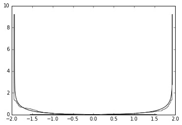
Refer to caption
Figure 3: The graph of a normalized random concave composition, with central part c=0c=0, of a large positive integer in the order of 10410^{4} along with the proposed limit shape given by Theorem 5.1. The sampling was done with respect to QqnQ_{q_{n}}.

6 Future work

We conclude with some open questions and possible threads of future work. First of all, we have assumed c=0c=0 throughout this paper but it would be interesting to derive the distribution of cc or allow c=α​nc=\alpha\sqrt{n} for some small α∈(0,1)\alpha\in(0,1), close to 00. In addition, the questions we have answered about concave compositions can also be asked of other compositions, such as strongly concave compositions (which was mentioned in [4]) or convex compositions. Another interesting direction would be to consider different measures on concave compositions, such as the Plancherel measure or the Ewens measure which have both been defined on partitions. Specifically, see if the asymptotic bounds for the perimeter, tilt and length are tighter under these and other measures.

Acknowledgements.
The authors would like to thank George Andrews, Paweł Hitczenko and Anatoly Vershik for their wonderful insights and helpful comments.

References

  • (1) Andrews, G.E.: The Theory of Partitions. Cambridge Mathematical Library. Cambridge University Press, Cambridge (1998). Reprint of the 1976 original
  • (2) Andrews, G.E.: Concave compositions. Electron. J. Combin. 18(2), Paper 6, 13 (2011)
  • (3) Andrews, G.E.: Concave and convex compositions. Ramanujan J. 31(1-2), 67–82 (2013). DOI 10.1007/s11139-012-9394-6. URL http://dx.doi.org.ezproxy.lib.uwf.edu/10.1007/s11139-012-9394-6
  • (4) Andrews, G.E., Rhoades, R.C., Zwegers, S.P.: Modularity of the concave composition generating function. Algebra Number Theory 7(9), 2103–2139 (2013). DOI 10.2140/ant.2013.7.2103. URL http://dx.doi.org/10.2140/ant.2013.7.2103
  • (5) Bender, E.A., Canfield, E.R.: Locally restricted compositions. I. Restricted adjacent differences. Electron. J. Combin. 12, Research Paper 57, 27 pp. (electronic) (2005). URL http://www.combinatorics.org/Volume_12/Abstracts/v12i1r57.html
  • (6) Bryson, J., Ono, K., Pitman, S., Rhoades, R.C.: Unimodal sequences and quantum and mock modular forms. Proc. Natl. Acad. Sci. USA 109(40), 16063–16067 (2012). DOI 10.1073/pnas.1211964109. URL http://dx.doi.org/10.1073/pnas.1211964109
  • (7) Chaganty, N.R., Sethuraman, J.: Strong large deviation and local limit theorems. Ann. Probab. 21(3), 1671–1690 (1993). URL http://links.jstor.org/sici?sici=0091-1798(199307)21:3<1671:SLDALL>2.0.CO;2-2&origin=MSN
  • (8) Corteel, S., Pittel, B., Savage, C.D., Wilf, H.S.: On the multiplicity of parts in a random partition. Random Structures Algorithms 14(2), 185–197 (1999). DOI 10.1002/(SICI)1098-2418(199903)14:2<185::AID-RSA4>3.3.CO;2-6. URL http://dx.doi.org/10.1002/(SICI)1098-2418(199903)14:2<185::AID-RSA4>3.3.CO;2-6
  • (9) Fristedt, B.: The structure of random partitions of large integers. Trans. Amer. Math. Soc. 337(2), 703–735 (1993). DOI 10.2307/2154239. URL http://dx.doi.org/10.2307/2154239
  • (10) Goh, W.M.Y., Hitczenko, P.: Average number of distinct part sizes in a random Carlitz composition. European J. Combin. 23(6), 647–657 (2002). DOI 10.1006/eujc.2002.0435. URL http://dx.doi.org/10.1006/eujc.2002.0435
  • (11) Goh, W.M.Y., Hitczenko, P.: Random partitions with restricted part sizes. Random Structures Algorithms 32(4), 440–462 (2008). DOI 10.1002/rsa.20191. URL http://dx.doi.org/10.1002/rsa.20191
  • (12) Grabner, P., Knopfmacher, A., Wagner, S.: A general asymptotic scheme for moments of partition statistics. preprint (2010)
  • (13) Heubach, S., Mansour, T.: Combinatorics of Compositions and Words. Discrete Mathematics and its Applications (Boca Raton). CRC Press, Boca Raton, FL (2010)
  • (14) Loève, M.: Probability Theory. Third edition. D. Van Nostrand Co., Inc., Princeton, N.J.-Toronto, Ont.-London (1963)
  • (15) MacMahon, P.A.: Combinatory Analysis. Vol. I, II (bound in one volume). Dover Phoenix Editions. Dover Publications, Inc., Mineola, NY (2004). Reprint of ıt An introduction to combinatory analysis (1920) and ıt Combinatory analysis. Vol. I, II (1915, 1916)
  • (16) Ngo, T.H., Rhoades, R.C.: Integer partitions, probabilities and quantum modular forms. preprint (2014)
  • (17) Petrov, F.: Two elementary approaches to the limit shapes of Young diagrams. Zap. Nauchn. Sem. S.-Peterburg. Otdel. Mat. Inst. Steklov. (POMI) 370(Kraevye Zadachi Matematicheskoi Fiziki i Smezhnye Voprosy Teorii Funktsii. 40), 111–131, 221 (2009). DOI 10.1007/s10958-010-9845-9. URL http://dx.doi.org.ezproxy.lib.uwf.edu/10.1007/s10958-010-9845-9
  • (18) Szalay, M., Turán, P.: On some problems of the statistical theory of partitions with application to characters of the symmetric group. I. Acta Math. Acad. Sci. Hungar. 29(3-4), 361–379 (1977)
  • (19) Temperley, H.N.V.: Statistical mechanics and the partition of numbers. II. The form of crystal surfaces. Proc. Cambridge Philos. Soc. 48, 683–697 (1952)
  • (20) Vershik, A.M.: Asymptotic combinatorics and algebraic analysis. In: Proceedings of the International Congress of Mathematicians, Vol. 1, 2 (Zürich, 1994), pp. 1384–1394. Birkhäuser, Basel (1995)
  • (21) Vershik, A.M.: Statistical mechanics of combinatorial partitions, and their limit configurations. Funktsional. Anal. i Prilozhen. 30(2), 19–39, 96 (1996). DOI 10.1007/BF02509449. URL http://dx.doi.org.ezproxy.lib.uwf.edu/10.1007/BF02509449
  • (22) Vershik, A.M., Kerov, S.V.: Asymptotic of the largest and the typical dimensions of irreducible representations of a symmetric group. Funktsional. Anal. i Prilozhen. 19(1), 25–36, 96 (1985)
  • (23) Wright, E.M.: Stacks. Quart. J. Math. Oxford Ser. (2) 19, 313–320 (1968)
  • (24) Wright, E.M.: Stacks. II. Quart. J. Math. Oxford Ser. (2) 22, 107–116 (1971)
  • (25) Wright, E.M.: Stacks. III. Quart. J. Math. Oxford Ser. (2) 23, 153–158 (1972)
  • (26) Yakubovich, Y.: Ergodicity of multiplicative statistics. J. Combin. Theory Ser. A 119(6), 1250–1279 (2012). DOI 10.1016/j.jcta.2012.03.002. URL http://dx.doi.org/10.1016/j.jcta.2012.03.002