Some Insights into the Geometry and Training of Neural Networks
Abstract
Neural networks have been successfully used for classification tasks in a rapidly growing number of practical applications. Despite their popularity and widespread use, there are still many aspects of training and classification that are not well understood. In this paper we aim to provide some new insights into training and classification by analyzing neural networks from a feature-space perspective. We review and explain the formation of decision regions and study some of their combinatorial aspects. We place a particular emphasis on the connections between the neural network weight and bias terms and properties of decision boundaries and other regions that exhibit varying levels of classification confidence. We show how the error backpropagates in these regions and emphasize the important role they have in the formation of gradients. These findings expose the connections between scaling of the weight parameters and the density of the training samples. This sheds more light on the vanishing gradient problem, explains the need for regularization, and suggests an approach for subsampling training data to improve performance.
1 Introduction
Neural networks have been successfully used for classification tasks in applications such as pattern recognition [2], speech recognition [10], and numerous others [25]. Despite their widespread use, the understanding of neural networks is still incomplete, and they often remain treated as black boxes. In this paper we provide new insights into training and classification by analyzing neural networks from a feature-space perspective. We consider feedforward neural networks in which input vectors are propagated through successive layers, each of the form
| (1) |
where is a nonlinear activation function that acts on an affine transformation of the output from the previous layer, with weight matrix and bias vector . Neural networks are often represented as graphs and the entries in vectors are therefore often referred to as nodes or units. There are three main design parameters in a feedforward neural network architecture: the number of layers or depth the network, the number of nodes in each layer, and the choice of activation function. Once these are fixed, neural networks are training by adjusting only the weight and bias terms.
Although most of the results and principles in this paper apply more generally, we predominantly consider neural networks with sigmoidal activation functions that are convex-concave and differentiable. To keep the discussion concrete we focus on a symmetrized version of the logistic function that acts elementwise on its input as
| (2) |
This function can be seen as a generalization of the hyperbolic tangent, with . We omit the subscript when , or when its exact value does not matter. For simplicity, and with some abuse of terminology we refer to as the sigmoid function, irrespective of the value of , and use the term logistic function for . Examples of several instances of and their first-order derivatives are plotted in Figure 1.
| (a) | (b) |
The activation function in the last layer has the special purpose of ensuring that the output of the neural network has a meaningful interpretation. The softmax function is widely used and generates an output vector whose entries are defined as
| (3) |
Exponentiation and normalization ensures that all output values are nonnegative and sum up to one, and the output of node can therefore be interpreted as an estimate of the posterior probability . That is, we can define the estimated probabilities as , where is a vector containing of network weight and bias parameters, and is the output at layer corresponding to input . The network parameters are typically learned from domain-specific training data. In supervised training for multiclass classification this training data comes in the form of a set of tuples , each consisting of a sample feature vector and its associated class label . Training is done by minimizing a suitably chosen loss function, such as
| (4) |
with the cross-entropy function
which we shall use throughout the paper. We denote the class corresponding to feature vector as , which, in practice, is known only for all points in the training set. For notational convenience we also write to mean . The loss function is highly nonconvex in making (4) particularly challenging to solve. However, even if it could be solved, care needs to be taken not to overfit the data to ensure that the network generalizes to unseen data. This can be achieved, for example, through regularization, early termination, or by limiting the model capacity of the network.
The outline of the paper is as follows. In Section 2 we review the definition of halfspaces and the formation of decision regions. In Section 3 we look at combinatorial properties of the decision regions, their ability to separate or approximate different classes, and possible generalizations. Section 4 analyzes the connection between the decision regions and the gradient with respect to the different network parameters. Topics related to the training of neural networks including backpropagation, regularization, the contribution of individual training samples to the gradient, and importance sampling are discussed in Section 5. We conclude the paper with a discussion and future work in Section 6.
Throughout the paper we use the following notational conventions. Matrices are indicated by capitals, such as for the weight matrices; vectors are denoted by lower-case roman letters. Sets are denoted by calligraphic capitals. Subscripted square brackets denote indexing, with , , and denoting respectively the -th entry of vector , the -th row of as a column vector, and the -th entry of matrix . Square brackets are also used to denote vector or matrix instances with commas separating entries within one row, and semicolon separating rows in in-line notation. When not exponentiated denotes the vector of all ones. The largest singular value of is denoted , from the context it will be clear that this is not a particular instance of the sigmoidal function . The vector , and norms refer to the one- and two norms; that is, the sum of absolute values and the Euclidean norm, respectively. There should be no confusion between this and the logistic function.
2 Formation of decision regions
Decision regions can be described as those regions or sets of points in the feature space that are classified as a certain class. Classification in neural networks is soft in the sense that it comes as a vector of posterior probabilities and, in case that is desirable, it is therefore not immediately obvious how to assign points to one class or another. Two possible definitions of decision regions for class are the set of points where the posterior probability is highest among the classes:
or exceeds a given threshold:
| (5) |
Although this section discusses the formation and role of decision regions and its boundaries, we will not use any formal definition of decision regions. However, the intuitive notion used closely follows definition (5).
As we will see in this section, decision regions are formed as input is propagated through the network. Even though the form (1) of all the layers is identical, we can nevertheless identify two distinct stages in region formation. The first stage defines a collection of halfspaces and takes place in the first layer of the network. The second stage takes place over the remaining layers in which intermediate regions are successively combined to form the final decision regions, starting with the initial set of halfspaces. The generation of halfspaces or hyperplanes in the first layer of the neural network and their combination in subsequent layers is well known (see for example [2, 16]). The formation of soft decision boundaries and some of their properties does not appear to have been studied widely. Some of the notions discussed next form the basis for subsequent sections, and we therefore review the two separate stages mentioned above in some detail, with a particular emphasis on the role of the sigmoidal activation function.
2.1 Definition of halfspaces
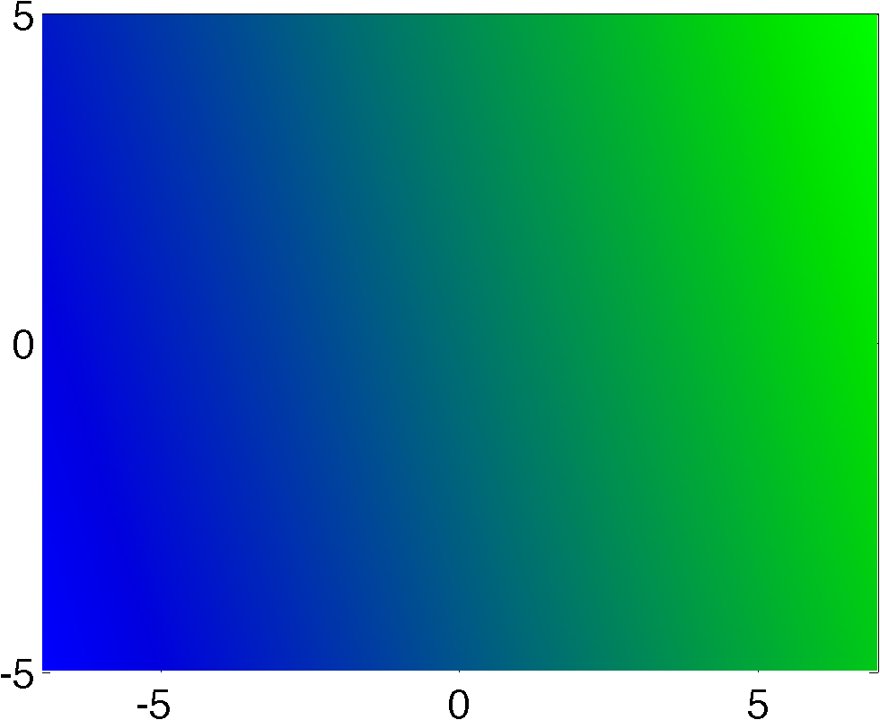
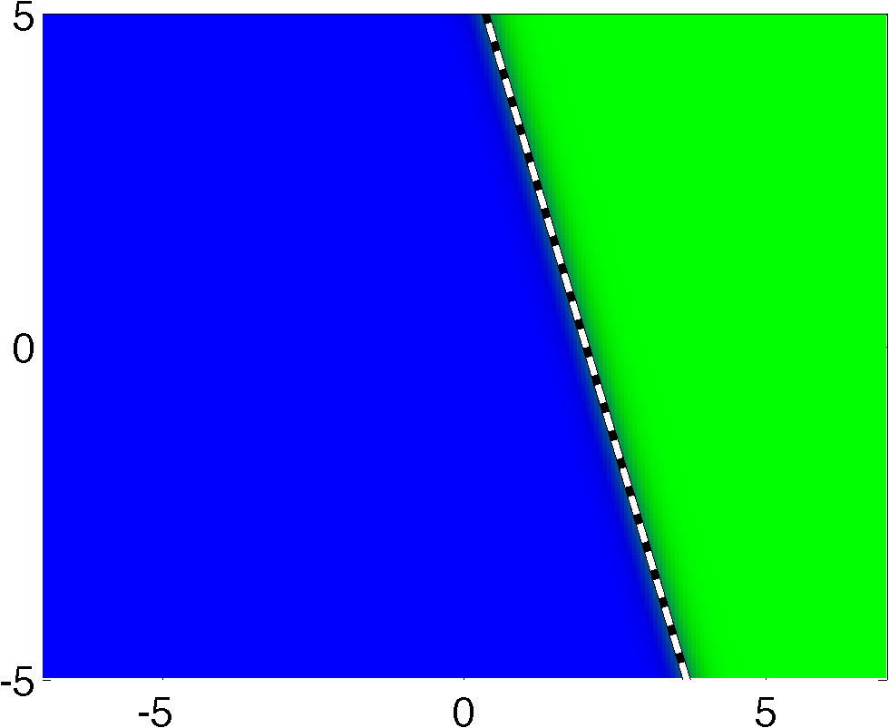
The output of the first layer in the network can be written as with . For an individual unit this reduces to , where corresponds to , the -th row of , and . When applied over all points of the feature space, the affine mapping generates a linear gradient, as shown in Figure 2(a). The output of a unit is then obtained by applying the sigmoid function to these intermediate values. When doing so, assuming throughout that , two prominent regions form: one with values close to and one with values close to . In between the two regions there is a smooth transition region, as illustrated in Figure 2(b). The center of the transition region consists of all feature points whose output value equal zero. It can be verified that this set is given by all points such that , and therefore describes a hyperplane. The normal direction of the hyperplane is given by , and the exact location of the hyperplane is determined by a shift along this normal, controlled by both and . The region of all points that map to nonnegative values forms a halfspace, and because the linear functions can be chosen independently for each unit, we can define as many halfspaces are there are units in the first layer. As the transition between the regions on either side of the hyperplane is gradual it is convenient to work with soft boundaries and interpret the output values as a confidence level of set membership with values close to indicating strong membership, those close to indicating strong non-membership, and with decreasing confidence levels in between. For simplicity we use the term halfspace for both the soft and sharp versions of the region.
 |
 |
 |
| (a) | (b) | (c) |
In addition to normal direction and location, halfspaces are characterized by the sharpness of the transition region. This property can be controlled in two similar ways (see also Section 5.2). The first is to scale both and by a positive scalar . Doing so does not affect the location or orientation of the hyperplane but does scale the input to the sigmoid by the same quantity. As a consequence, choosing shrinks the transition region, whereas choosing causes it to widen. The second way is to replace the activation function by . Scaling only affects the sharpness of the transition in the same way, but also results in a shift of the hyperplane along the normal direction whenever . Note however that the activation functions are typically fixed and the properties of the halfspaces are therefore controlled only by the weight and bias terms. Figure 2(c) illustrates the sharpening of the halfspace and the use of to change its location.
2.2 Combination of intermediate regions
The second layer combines the halfspace regions defined in the first layer resulting in new regions in each of the output nodes. In case step-function activation functions are used, the operations used to combine the regions correspond to set operations including complements (c), intersection (), and unions (). The same operations are used in subsequent layers, thereby enabling the formation of increasingly complex regions. The use of a sigmoidal function instead of the step function does not significantly change the types of operations, although some care needs to be taken.
Some operations are best explained when working with input coming from the logistic function (with values ranging from 0 to 1) rather than from the sigmoid function (ranging from -1 to 1). Note however that output from a sigmoid function can easily be mapped to the output from a logistic function, and vice versa, by appropriately scaling the weight and bias terms in the next layer. Any linear operation on the logistic output then becomes with and . In other words, with appropriate changes in and we can always choose which of the two activation functions the input comes from, regardless of which function was actually used.
2.2.1 Elementary Boolean operations
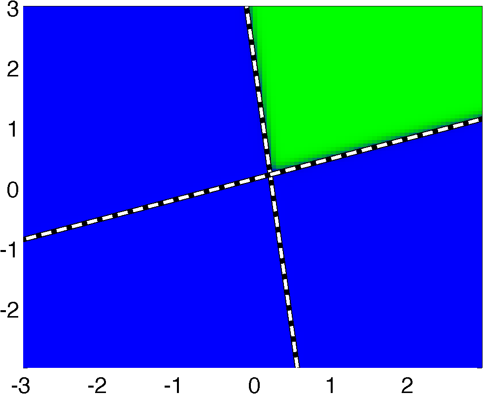
To make the operations discussed in this section more concrete we apply them to input generated by a first layer with the following parameters:
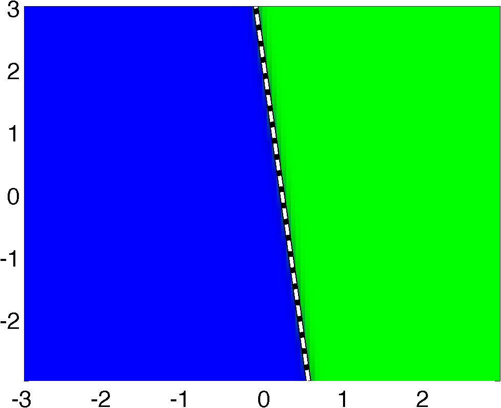
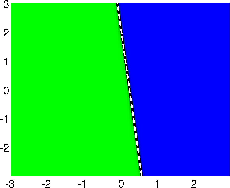
The two resulting halfspace regions and are illustrated in Figures 3(a) and 3(b). For simplicity we denote the parameters for the second layer by and , omitting the subscripts. In addition, we omit all entries that are not relevant to the operation and apply appropriate padding with zeros where needed is implied.
 |
 |
 |
| (a) Region | (b) Region | (c) Complement: |
 |
 |
 |
| (d) | (e) | (f) |
| ( xor ) |
Constants
Constants can be generated by choosing and choosing a sufficiently large positive or negative offset values. For example, choosing gives a region that spans the entire domain (representing the logical true), whereas choosing results in the empty set (or logical false).
Unary operations
The simplest unary operation, the (Boolean) identity function, can be defined as
This function works well when used in conjunction with a step function, but has an undesirable damping effect when used with the sigmoid function: input values up to 1 are mapped to output values up to , and likewise for negative values. While such scaling may be desirable in certain cases, we would like to preserve the clear distinction between high and low confidence regions. We can do this by scaling up , which amplifies the input to the sigmoid function and therefore its output. Choosing , for example, would increase the maximum confidence level to . As noted towards the end of Section 2.1, the same can be achieved by working with the activation function , and to avoid getting distracted by scaling issues like these we will work with throughout this section. We note that the identity function can be approximated very well by scaling down the input and taking advantage of the near-linear part of the sigmoid function around zero. The output can then be scaled up again in the next layer to achieve the desired result. Similar to the identity function, we define the complement of a set as
The application of this operator to is illustrated in Figure 3(c). Just to be clear, note that in this case the full parameters to the second layer would be and .
Binary operations
When taking the intersection of regions and we require that the output values of the corresponding units in the network sum up to a value close to two. This is equivalent to saying that when we subtract a relatively high value, say , from the sum, the outcome should remain positive. This suggests the following parameters for binary intersection:
We now combine the intersection and complement operations to derive the union of two sets, and to illustrate how complements of sets can be applied during computations. By De Morgan’s law, the union operator can be written as . Evaluation of this expression is done in three steps: taking the individual complements of and , applying the intersection, and taking the complement of the result. This can be written in linear form as
Substituting the weight and bias terms and simplifying yields parameters for the union:
2.2.2 General -ary operations
We now consider general operations that combine regions from more than two units. It suffices to look at a single output unit with weight vector and bias term . Any negative entry in mean that the corresponding input region is negated and that its complement is used, whereas zero valued entries indicate that the corresponding region is not used. Without loss of generality we assume that all input regions are used and normalized such that all entries in can be taken strictly positive. We again start by looking at the idealized situation where inputs are generated using a step function with outputs -1 or 1. When is the vector of all ones, and out of inputs are positive we have . Choosing activation level therefore ensures that the output of the unit is positive whenever at least out of inputs are positive. As extreme cases of this we obtain the -ary intersection with , and the -ary union by choosing . Weights can be adjusted to indicate how many times each region gets counted.
 |
 |
 |
| (a) | (b) | (c) |
 |
 |
 |
| (d) | (e) | (f) |
It was noted by Huang and Littmann [13] that complicated and highly non-intuitive regions can be formed with the general -ary operations, even in the second layer. As an example, consider the eight hyperplane boundaries plotted in Figure 4(a). The weight assigned to each hyperplane determines the contribution to each cell that lies within the enclosed halfspace. The total contributions for each cell shown in Figure 4(a) represent the total weight obtained when using weight two to the outer hyperplanes and a unit weight for the inner hyperplanes, combined with step function input from 0 to 1. Adding up values for so many regions in a single step worsens the scaling issue mentioned for the unitary operator: In this case choosing a threshold of leads to values ranging from to before application of the sigmoid function. Using and for amplification with different weight vectors and threshold values we obtain the regions shown in Figures 4(b) to 4(d).
Removing the large amplification factor in the second layer can lead to regions with low or varying confidence levels. For the mixed weights example, using and threshold causes the intended region to have four distinct confidence levels, as shown in Figure 4(e). Low weights can also be leveraged to obtain a parsimonious representation of smooth regions that would otherwise require the many more halfspaces. An example of this is shown in Figure 4(f) in which the four outer halfspaces with soft boundaries are combined to form a smooth circular region.
2.3 Boolean function representation using two layers
As seen from Section 2.2.1 neural networks can be used to take the union of intersections of (possibly negated) sets. In Boolean logic this form is called disjunctive normal form (DNF), and it is well known that any Boolean function can be expressed in this form (see also [1]). Likewise we could reverse the order of the union and intersection operators and arrive at conjunctive normal form (CNF), which is equally powerful. Two-layer networks are, in fact, far stronger than this and can be used to approximate general smooth functions. More information on this can be found in [2, Sec. 4.3.2].
2.4 Boundary regions and amplification

The use of sigmoidal nonlinearity functions leads to continuous transitions between different regions. The center of the transition regions for a node can be defined as the set of feature points for which the output of that node is zero. Given input for some node at depth we first form , then subtract the bias , and apply the sigmoid function. The output is zero if and only if , and the transition center therefore corresponds to the level set of at . For a fixed we can thus control the location of the transition by changing . As an example consider a two-level neural network with the first layer parameterized by , , and the second layer by , . Writing the input vector as it can be seen that , as illustrated in Figure 5. All values greater than will be mapped to positive values and, as discussed in Section 2.2.1, we again see that choosing approximates the intersection of the regions and , whereas choosing approximates the union (indicated in the figure by the lines at ). What we are interested in here is the location of the transition center. Clearly, making the intersection more stringent by increasing causes the boundary to shift and the resulting region to become smaller. Another side effect is that the output range of the second layer, which is given by , changes. Choosing close to , the supremum of the input signal, means that the supremum of the output is close to zero, whereas the infimum nearly reaches -1. To obtain larger positive confidence levels in the output, without shifting the transition center, we need to amplify the input by scaling and by some . In Figure 6 we study several aspects of the boundary region corresponding to the setting used for Figure 5, with the addition of scaling parameter . For a given we choose such that the maximum output of is . Figures 6(a)–(c) show the transition region with values ranging from and along with the center of the transition with value and the region with values exceeding . Figure 6(d) shows the required scaling factors.
The ideal intersection of the two regions coincides with the positive orthant and we define the shift in the transition boundary as the limit of the -coordinate of the zero crossing as goes to infinity, giving
The resulting shift values are show in Figure 6(e). Another property of interest is the width of the transition region. Similar to the shift we quantify this as the difference between the asymptotic -coordinates of the and level set contours as goes to infinity. We plot the results for several multiples of in Figure 6(f). As expected, we can see that larger amplification reduces the size of the transition intervals. The vertical dashed line indicates the critical value of at which the contour becomes diagonal () causing the transition width to become infinite. The same phenomenon happens at smaller when the multiplication factor is higher. Note that this break down is due only to the definition of the transition width; the transition region itself remains perfectly well defined throughout.
| (a) | (b) | (c) |
| (d) | (e) | (f) |
2.5 Continuous to discrete
The level-set nature of applying the nonlinearity as illustrated in Figure 5 allows the generation of decision boundaries that look very different from any one of those used for its input. One example of this was shown in Figure 4(f) in which a circular region was generated by four axis-aligned hyperplanes, and we now describe another. Consider the two hyperplanes in Figures 7(a,b), generated in the first layer with respectively , , and , . The small weights and the limited domain size cause the input values to the nonlinearity to be small. As a result, the sigmoid operates in its near-linear region around the origin and therefore resembles scalar multiplication. Consequently, because the normals of the first layers form a basis, we can use the second layer to approximate any operation that would normally occur in the first layer. For example we can choose and to generate a close approximation of a hyperplane at angle (up to a scaling factor this weight matrix is formed by multiplying the desired normal vector by the rotation on the inverse of the weight matrix of the first layer). The resulting regions of the second layer are shown in Figures 7(c,d) for and , respectively. This illustrates that, although somewhat contrived, it is technically possible, at least locally, to change hyperplane orientation after the first layer.
As decision regions propagate and form through one or more layers with modest or large weights, their boundaries become sharper and we see a gradual transition from continuous to discrete network behavior. In the continuous regime, where the transitions are still gradual, the decision boundaries emerge as level sets of slowly varying smooth functions and therefore change continuously and considerably with the choice of bias term. As the boundary regions become sharper the functions tend to piecewise constant causing the level sets to change abruptly only at several critical values while remaining fairly constant otherwise, thus giving more discrete behavior. In Figures 7(e,f) we show intermediate stages in which we scale the weights in the first layer Figures 7(d) by a factor of 10 and 20, respectively. In addition, it can be seen that scaling in this case does not just sharpen the boundaries, but actually severely distorts them. Finally, it can be seen that the resulting region becomes increasingly diagonal (similar to its sharpened input) as the weights increase. This again emphasizes the more discrete nature of region combinations once the boundaries of the underlying regions are sharp.
 |
 |
 |
| (a) | (b) | (c) |
 |
 |
 |
| (d) | (e) | (f) |
2.6 Generalized functions for the first layer
The nodes in the first layer define geometric primitives, which are combined in subsequent layers. Depending on the domain it may be desirable to work with primitives other than halfspaces, or to provide a set of different types. This can be achieved by replacing the inner products in the first layer by more general functions with training examples and (possibly shared) parameters . The traditional hyperplane is given by
For ellipsoidal regions we could then use
More generally, it is possible to redefine the entire unit by replacing both the inner-product and the nonlinearity with a general function to obtain, for example, a radial-basis function unit [15]. In Figure 8 we illustrate how a mixture of two types of geometric primitives can form regions that cannot be expressed concisely with either type alone.
 |
 |
 |
| (a) Linear, | (b) Gaussian, | (c) |
3 Region properties and approximation
The hyperplanes defined by the first layer of the neural network partition the space into different regions. In this section we discuss several combinatorial and approximation theoretic properties of these regions.
3.1 Number of regions
One of the most fundamental properties to consider is the maximum number of regions into which can be partitioned using hyperplanes. The exact maximum is well known to be
| (6) |
and is attained whenever the hyperplanes are in general position [21, p.39]. With the hyperplanes in place, the subsequent logic layers in the neural network can be used to identify each of these regions by taking the union of (complements of) halfspaces. Individual regions can then be combined using the union operator.
3.2 Approximate representation of classes
3.2.1 Polytope representation
When the set of points belonging to a class form a bounded convex set, we can approximate it by a polytope given by the bounded intersection of a finite number of halfspaces. The accuracy of such an approximation can be expressed as the Hausdorff distance between the two sets, defined as:
with
For a given class of convex bodies , denote . We are interested in when , the set of all polytopes in with at most facets (i.e., generated by the intersection of up to halfspaces), and in particular how it behaves as a function of . The following result obtained independently by [4, 8] is given in [5]. For every convex body there exists a constant such that
More interesting perhaps is a lower bound on the approximation distance. For the unit ball we have the following:
Theorem 3.1.
Let denote the unit ball in . Then for sufficiently large there exists a constant such that
Proof.
For large enough there exists a polytope with facets and . Each of the facets in is generated by a halfspace, and we can use each halfspace to generate a point on the unit sphere in such that the surface normal at that point matches the outward normal of the halfspace. We denote the set of these points by , with . Now, take any point on the unit sphere. From the definition of it follows that the maximum distance between and the closest point on one of the hyperplanes bounding the halfspaces is no greater than . From this it can be shown that the distance to the nearest point in is no greater than . Moreover, because the choice of was arbitrary, it follows that defines an -net of the unit sphere. Lemma 3.2 below shows that the cardinality . Substituting gives
∎
Lemma 3.2.
Let be an -net of the unit sphere in with , then
Proof.
By definition of the -net, we obtain a cover for by placing balls of radius at all . The intersection of each ball with the sphere gives a spherical cap. The union of the spherical caps covers the sphere and times the area of each spherical cap must therefore be at least as large as the area of the sphere. A lower bound on the number of points in is therefore obtained by the ratio between the area of the sphere and that of the spherical cap (see also [24, Lemma 2]). Denoting by the half-angle of the spherical cap it follows from [14, Corollary 3.2(iii)] that satisfies
whenever . This bound can be substituted into the second term above to obtain , and it can be verified to hold whenever . It further holds that which, after rewriting, gives the desired result. ∎
3.2.2 More efficient representations
From Theorem 3.1 we see that a large number of supporting hyperplanes is needed to define a polytope that closely approximates the unit -norm ball. Approximating such a ball or any other convex sets by the intersection of a number of halfspaces can be considered wasteful, however, since it uses only a single region out of the maximum given by (6). This fact was recognized by Cheang and Barron [6], and they proposed an alternative representation for unit balls that only requires halfspaces—far fewer than the conventional . The construction is as follows: given a set of suitably chosen halfspaces and the indicator function which is one if and zero otherwise. Typically these halfspaces are used to define polytope , that is, the intersection of all halfspaces. The (non-convex) approximation proposed in [6] is of the form
which consists of all points that are contained in at least halfspaces. This representation is shown to provide far more efficient approximations, especially in high dimensions. As described in Section 2.2.2, this construction can easily be implemented as a neural network. A similar approximation for the Euclidean ball, which also takes advantage of smooth transition boundaries is shown in Figure 4(f).
3.3 Bounds on the number of separating hyperplanes
In many cases, it suffices to simply distinguish between the different classes instead of trying to exactly trace out their boundaries. Doing so may reduce the number of parameters and additionally help reduce overfitting. The bound in Section 3.1 gives the maximum number of regions that can be separated by a given number of hyperplanes. Classes found in practical applications are extremely unlikely to exactly fit these cells, and we can therefore expect that more hyperplanes are needed to separate them. We now look at the maximum number of hyperplanes that is needed.
3.3.1 Convex sets
In this section we assume that the classes are defined by convex sets whose intersection is either empty or of measure zero. We are interested in finding the minimum number of hyperplanes needed such that each pair of classes is separated by at least one of the hyperplanes. In the worst case, a hyperplane is needed between any pair of classes, giving a maximum of hyperplanes, independent of the ambient dimension. That this maximum can be reached was shown by Tverberg [23] who provides a construction due to K.P. Villanger of a set of lines in such that any hyperplane that separates one pair of lines, intersects all others. Here we describe a generalization of this construction for odd dimensions .
Theorem 3.3.
Let be a full-spark[7] matrix with blocks of size , with odd . Let , be vectors in such that is full rank for all . The subspaces
are pairwise disjoint and any hyperplane separating and , , intersects all , .
Proof.
Any pair of subspaces and intersects only if there exist vectors , such that
It follows from the assumption that is full rank, that no such two vectors exist, and therefore that all subspaces are pairwise disjoint.
Any hyperplane separating and is of the form . To avoid intersection with we must have for all , which is satisfied if an only if . It follows that we must also have , and therefore that is a normal vector to the -subspace spanned by . From the full-spark assumption on it follows that for all , which shows that intersects the corresponding . The result follows since the choice of and was arbitrary. ∎
Random matrices and vectors with entries i.i.d. Gaussian satisfy the conditions in Theorem 3.3 with probability one, thereby showing the existence of the desired configurations. A simple extension of the construction to dimension is obtained when generating subspaces by matrices , formed by appending a row of zeros to and adding a column corresponding to the last column of the identify matrix, and vectors . Pach and Tardos [18] further show that the lines in the construction described by Tverberg can be replaced by appropriately chosen unit segments. Adding a sufficiently small ball in the Minkowski sense then results in bounded convex sets with non-empty interior whose separation requires the maximum hyperplanes.
3.3.2 Point sets
When separating a set of points, the maximum number of hyperplanes needed is easily seen to be ; we can cut off a single extremal point of subsequent convex hulls until only a single point is left. This maximum can be reached, for example when all points lie on a straight line. For a set of points in general position, it is shown in [3] that the maximum number of hyperplanes needed satisfies
Based on this we can expect the number of hyperplanes needed to separate a family of unit balls to be much smaller than the maximum possible , whenever .
3.3.3 Non-convex sets
The interface between two non-convex sets can be arbitrarily complex, which means that there are no meaningful bounds on the number of hyperplanes needed to separate general sets.
4 Gradients
Parameters in the neural network are learned by minimizing a loss function over the training set, using for example stochastic gradient descent on the formulation shown in (4). The gradient of such a loss function decouples over the training samples and can be written as
| (7) |
where each term can be evaluated using backpropagation [20]. The idea of the section is to explore how points contribute when they are part of a training set. That is, for a given parameter set , and with the class information assumed to be known, we are interested in ; the behavior of as a function of over the entire feature space. We will see that some points in the training set contribute more to the gradient than others. So, instead of just looking at the total gradient, we look at the contribution to the gradient of each point: points that have a large relative contribution to the gradient can be said to be more informative than those that do not contribute much (the amount of contribution of each point typically changes during optimization). Throughout this and the next section we use the word ‘gradient’ loosely and also use it to refer to blocks of gradient entries corresponding to the parameters a layer, individual entries, or the gradient field of those quantities over the entire feature space. The exact meaning should be clear from the context.
4.1 Motivational example
We illustrate the relative importance of different training samples using a simple one-dimensional example. We define a basic two-layer neural network in which the first layer defines a hyperplane with nonlinearity , and in which the second layer applies the identity function follow by nonlinearity for amplification (for simplicity we look only at one class and use a logistic function instead of the softmax function). Choosing and defines the region shown in Figure 9(a). Now, suppose that all points belong to the same class and should therefore be part of this region. Intuitively, it can be seen that slight changes in the location of the hyperplane or in the steepness of the transition will have very little effect on the output of the neural network for input points , say, since values close to one or zero remain so after the perturbation. As such, we expect that in these regions the gradient with respect to and will be small. For points in the transition region the change will be relatively large, and the gradient at those points will therefore be larger. This suggests that training points away from the transition region provide little information when deciding in which direction to move the hyperplane and how sharp the transition should be; this information predominantly comes from the training points in the transition region.
| (a) | (b) | (c) |
More formally, consider the minimization of the negative log likelihood loss function for this network, given by
For the gradient, we need the derivative of the sigmoid function, with
and the derivative of the negative log of the logistic function:
Combining the above we have
with . The loss function and partial derivatives with respect to and are plotted in Figure 9(b) and (c). The vertical lines in plot (c) indicate where the gradients fall below one percent of their asymptotic value. As expected, points beyond these lines do indeed contribute very little to the gradient, regardless of whether they are on the right or the wrong side of the hyperplane.
4.2 General mechanism
For the contribution of each sample to the gradient in general settings we need to take a detailed look at the backpropagation process. This is best illustrated using a concrete three-layer neural network:
| (8) |
Denoting by the negative log likelihood of , the forward and backward passes through the network can be written as
| (9) |
where the left and right columns respectively denote the stages in the forward and backward pass. The regions formed during the forward pass are shown in Figure 10. With this, the partial differentials with respect to weight matrices and bias vectors are of the following form:
| (10) |
 |
 |
 |
| (a) | (b) | (c) |
 |
 |
 |
| (d) | (e) | (f) |
 |
 |
 |
| (g) | (h) | (i) |
We now analyze each of the backpropagation steps to explain the relationship between the regions of high and low confidence at each of the neural network layers and the gradient values or importance of different points in the feature space. In all plots we only show the absolute values of the quantities of interest because we are mostly interested in the relative magnitudes over the feature space rather than their signs. After a forward pass through the network we can evaluate the loss function and its gradients, shown in Figure 11(a). In this particular example we have , so we only show the former. Given we can use (10) to compute the partial differentials of with respect to the entries in and . The partial differential with respect to simply coincides with , and is therefore not very interesting. On the other hand, we see that the partial differential with respect to is formed by multiplying with the output value . When looking at the feature space representation for the specific case of and using absolute values, this corresponds to the pointwise multiplication of the values in Figure 11(a) with the mask shown Figure 11(b). This multiplication causes the partial differential to be reduced in areas of low confidence in . In addition, it causes the partial differential to vanish at points at the zero crossing of the boundary regions, as illustrated by the white curve in the upper-right corner of Figure 11(c).
 |
 |
 |
| (a) | (b) | (c) |
 |
 |
 |
| (d) | (e) Mask: | (f) |
 |
 |
 |
| (g) | (h) | (i) |
 |
 |
 |
| (j) Mask: | (k) | (l) |
 |
 |
 |
| (a) | ||
 |
 |
 |
| (b) | ||
 |
 |
 |
| (c) | ||
In the next stage of the backpropagation we multiply by the transpose of to obtain , shown in Figure 11(d). As an intermediate value itself is not used, but it is further backpropagated though multiplication by to obtain . As illustrated in Figure 1(a), the gradient of the sigmoid is a kernel around the origin, and when applied to , the preimage of under , it emphasizes the regions of low confidence and suppresses the regions of high confidence. This can be seen when comparing the mask for , shown in Figure 11(e), with the corresponding region shown in Figure 10(d). The result obtained with multiplication by the mask is illustrated in Figure 11(f) and shows that backpropagation of the error is most predominant in the boundary region as well as in some regions where it was large to start with (most notably at the top of the bottom-left quadrant). From here we can compute the partial differential with respect to the entries of though multiplication by , which again damps values around the transition region, and backpropagate further to get , as shown in Figures 11(g)–(i). To obtain , we need to multiply by the mask corresponding to the preimage of the regions in . Unlike all other layers, these values are unbounded in the direction of the hyperplane normal and, as shown in Figure 11(j), result in masks that vanish away from the boundary region. Multiplication by the mask corresponding to gives shown in Figure 11(k). We finally obtain the partial differentials with respect to the entries in by multiplying by the corresponding entries in . For the first layer this stage actually amplifies the gradient entries whenever the corresponding coordinate value exceeds one in absolute value. In subsequent layers the maximum values of lie in the -1 to 1 output range of the sigmoid function and can therefore only reduce the resulting gradient components.
In Figure 12(a) we plot the maximum absolute gradient components for each of the three weight matrices. It is clear that the partial differentials with respect to are predominant in misclassified regions, but also exist outside of this region in areas where the objective function could be minimized further by increasing the confidence levels (scaling up the weight and bias terms). In the second layer, the backpropagated values are damped in the regions of high confidence and concentrate around the decision boundaries, which, in turn, are aligned with the underlying hyperplanes. Finally, in the first layer, we see that gradient values away from the hyperplanes have mostly vanished as a result of multiplication with the sigmoid gradient mask, despite the multiplication with potentially large coordinate values. Overall we see the tendency of the gradients to become increasingly localized in feature space towards the first layer. The boundary shifts we discussed in Section 2.4 can lead to additional damping, as the sigmoid derivative masks no longer align with the peaks in the gradient field. Scaling of the weight and bias is detrimental to the backpropagation of the error (a phenomenon that is also known as saturation of the sigmoids [15]) and can lead to highly localized gradient values. This is illustrated in Figures 12(b) and (c) where we scale all weight and bias terms by a factor of and , respectively. Especially in deep networks it can be seen that a single sharp mask in one of the layers can localize the backpropagating error and thereby affect all preceding layers. These figures also show that the increased scaling of the weights not only leads to localization, but also to attenuation of the gradients. In the first layer this is further aided by the multiplication with the coordinate values. Summarizing, we see that the repeated multiplication by the masks generated by the derivative of the activation function tends to localize gradients. Multiplication with in the back propagation mixes the regions with large gradients, but the location of these regions does not otherwise change. Finally, we note that the above principles are not restricted to the sigmoid or hyperbolic tangent functions. However, for activation functions where the gradient masks as not localized, for example for rectified linear units of the form , the vanishing gradient problem is less of a problem.
5 Optimization
In the previous section we studied how individual training samples contribute to the overall gradient (7) of the loss function. In this section we take a closer look at the dynamic behavior and the changing relevance of training samples during optimization over the network parameter vector . The parameter updates are gradient-descent steps of the form
| (11) |
with learning rate . The goal of this section is to clarify the relationships between the training set and the optimization process of the network parameters. To keep things simple we make no effort to improve the efficiency of the optimization process and, unless noted otherwise, we use a fixed learning rate with a moderate value of . Likewise, we compute the exact gradient using the entire training set instead of using an approximation based on suitably chosen subsets, as is done in practically favored stochastic gradient descent (SGD) methods. Note, however, that the mechanisms exposed in this section are general enough to carry over to these and other methods without substantial changes. Similar findings may moreover apply to other models. Throughout this section we place a particular emphasis on the first layer of the neural network. To illustrate certain mechanisms it often helps to keep parameters of subsequent layers fixed. In this case it is implied that the corresponding entries in the gradient update in (11) are zeroed out.
5.1 Sampling density and transition width
To investigate the roles of sampling density and transition width we start with a very simple example with feature vectors , and two classes: one to the left of the -axis (first entry is negative), and one to the right. Example training sets with samples in each of the two classes are plotted in Figure 13(a) and (b). Given such training sets we want to learn the classification using a neural network with a single hidden layer consisting of one node. To ensure that the classes are well defined we place four training samples—two for each class– near the interface of the two classes and sample the remaining points to the left and right of these points. Unless stated otherwise we keep all network parameters fixed except for the weights and bias terms in the first layer.
5.1.1 Sampling density
In the first experiment we study how the number or density of training points affects the optimization. We initialize the network with parameters
and keep the parameters in the second layer fixed. Parameter is chosen such that the initial hyperplane goes through the point . Training sets consist of samples, including the four at the interface, and are chosen such that the number of points in each class differs by at most one. Figures 13(a) and (b) illustrate such sets for , and , respectively. The hyperplane is indicated by a thick black line, bordered with two dashes lines which indicate the location where the output of the first layer is equal to . Figure 13(c) shows the magnitude of the partial differential with respect to at the initial parameter setting over the entire domain. The gradient is then computed as the average of the gradient values evaluated at the individual training samples. As a measure of progress we can look at the area of the misclassified region, i.e., the region between the -axis and the hyperplane (note this quantity does not include information about the confidence levels of the classification). Figure 13(e) shows this area as a function of iteration for different sampling densities. The shape of the loss function curves are very similar to these and we therefore omit them here. For and the area of the misclassified region steadily goes down to zero, although the rate at which it does so gradually diminishes. Although not apparent from the curves, this phenomenon happens for all the training sets used here and we will explain exactly why this happens in Section 5.2. Progress for and appears much less uniform and exhibits pronounced stages of fast and slow progress. The reason for this is a combination of the sampling density and the localized gradient. From Figure 13(c) we can see that the gradient field is concentrated around the hyperplane, with peak values slightly to the left of the hyperplane. When the sampling density is low it may happen that none of the training samples is close to the hyperplane. When this happens, the gradient will be small, and consequently progress will be slow. When one or more points are close to the hyperplane, the gradient will be larger and progress is faster. Figure 13(f) shows the rate of change in the area of the misclassified region along with the distance between the hyperplane and its nearest training sample for . It can be seen that the rate increases as the hyperplane moves towards the training sample, with the peak rate happening just before the hyperplane reaches the point. After that the rate gradually drops again as the hyperplane slowly moves further away from the sample. This is precisely the state at 300,000 iterations, which is illustrated in Figure 13(d). For , we find ourselves in the same situation right at the start. Initially we move away from a single training point, but as a consequence of the low sampling density, no other sampling points are nearby, causing a prolonged period of very slow progress. The discrete nature of training samples is less pronounced when the overall sampling density is high, or when the transition widths are large.
| (a) | (b) |
 |
|
| (c) | (d) |
| (e) | (f) |
5.1.2 Transition width
To illustrate the effect of transition widths, we used the setting with 3,200 samples as described above, but scaled the row vector of the initial to have Euclidean norm ranging from 1 to 100. In each case we adjust such that the initial hyperplane goes through the point . As shown in Figure 14(a), the misclassified area reaches zero almost immediately when is scaled to have unit norm. In other words, the hyperplane is placed correctly in this case after only 3,260 iterations. As the norm of the initial increases, it takes longer to reach this point: for an initial norm of it takes some 72,580 iterations, whereas for an initial norm of it takes over 300,000. Accordingly, we see from Figure 14(b) that the loss also drops much faster for small weights than it does for large weights. However, once the hyperplane is in place, the only way to decrease the loss is by scaling the weights to improve the confidence. This process can be somewhat slow when the weights are small and the hyperplane placement is finalized (as is the case when we start with small initial weights). As a result, the setup with initial weight of 25 eventually catches up with the earlier two, simply because it has a much sharper transition at the boundary as the hyperplane finally closes in to the right location.
| (a) | (b) |
| (c) | (d) |
The reason why the hyperplane moves faster for small initial weights is twofold. First, the transition width and support of the gradient field are larger. As a result, more sample points contribute to the gradient, leading to a larger overall gradient value. This is shown in Figures 14(c) and (d) in which we plot the norm of the gradients with respect to and when choosing , and such that the hyperplane goes through the given location on the -axis. The gradients with respect to either parameters are larger for smaller . (Unlike in Figure 12, the localization of the gradient here is due only to scaling of the weights in the first layer; the intensity of the gradient field therefore remains unaffected.) As the value of increases, the curves in Figures 14(c) become more linear. For those values the gradient is highly localized and, aside from the scaling by the training point coordinates, largely independent of the hyperplane location. The gradient with respect to does not include this scaling and therefore remains nearly constant as long as the overlap between the transition width and the class boundary is negligible. As the hyperplane moves into the right place, the gradient vanishes due to the cancellation of the contributions from the training points from the classes on either side of it. The curves for and, to a lesser extent for , show minor aberrations due to a relatively low sampling density compared to the transition width. Second, having larger gradient values for smaller weights means that the relative changes in weights are amplified, thereby allowing the hyperplane to move faster.
5.2 Controlling the parameter scale
In this section we work with a modified version of the domain shown in Figure 13(a). In particular, we change the horizontal extent from to , and randomly select 250 training samples uniformly at random for each of the two classes (thus leaving the sampling density unaffected compare to the original ). As a first experiment we optimize a three-layer network with initial parameters:
| (12) |
When we look at the row-norms of the weight matrices, plotted in Figure 15(a), we can see that all of them are growing. This growth can help improve the final confidence levels, but can be detrimental during the optimization process, especially when it occurs in the layers between the first and the last. Indeed, we can see from Figure 15(b) that the hyperplane never quite reaches the origin, despite the large number of iterations. As illustrated in Figure 12, scaling of the weight and bias terms leads to increasingly localized gradients. When the training sample density is low compared to the size of the regions where the gradient values are significant, it can easily happen that no significant values from the gradient field are sampled into the gradient. This applies in particular to the first several layers (depending on the network depth) where the gradient fields become increasingly localized (though not necessarily small) as a result of the sigmoidal gradient masks that are applied during back propagation, along with shifts in the boundary regions. This ‘vanishing gradient’ phenomenon can prematurely bring the training process to a halt; not because a local minimum is reached, but simply because the sampled gradient values are excessively small11 1 Small gradients can also be due to cancellations in the various contributions. In practice, and especially when classes mix in a boundary zone, the small gradient can be expected to be due to a combination of the two effects.. Scaling of the parameters in any layer except the last can cause the gradient field to become highly localized for the current and all preceding layers. This can cause a cascading effect in which suboptimal parameters in a stalled first layer lead to further parameter scaling in later layers, eventually causing the second layer to stall, and so on. To avoid this, we need to control the parameter scale during optimization.
Parameter growth can be controlled by adding a regularization or penalty term to the loss function, or by imposing explicit constraints. Extending (4) we could use
| (13) |
where is a regularization function, and are constraint functions. The discussions so far suggest some natural choices of functions for different layers. The function in the first layer should generally be based on the (Euclidean) norm of each of the rows in , such as their sum, maximum, or norm. The reason for this is that each row in defines the normal of a hyperplane, and using any function other than an norm may introduce a bias in the hyperplane directions due to a lack of rotational invariance. For subsequent layers (except possibly the last layer) we may want to ensure that the output cannot be too large. In the worst case, each input from the previous layer is close to or , and we can limit the output value by ensuring that the sum of absolute values, i.e., the norm, of each row in is sufficiently small. Of course, the corresponding value in could still be large, which may suggest adding a constraint that for each row . However, this constraint is non-convex and may impede sign changes in . The use of an norm-based penalty or constraint on intermediate layers has the additional benefit that it leads to sparse weight matrices, which can help reduce model complexity as well as evaluation cost.
| (a) | (b) |
As an illustration of the effect of regularization on the first layer we consider the setting as given in (12), but with the second layer removed. We optimize the weight and bias terms in the first layer using the standard formulation (4), as well as those in (13) with or . For simplicity we keep all other network parameters fixed. Optimization in the constrained setting is done using a basic gradient projection method with step size fixed to 0.01, as before. The results are show in Figure 16. When using the standard formulation we see from Figure 16(a) that, like above and in Figures 13(a,d), the norm of the row in keeps growing. This is explained as follows: suppose the hyperplane is vertical with of the form , and . Then the area of the misclassified region is . We can therefore reduce the misclassified area (and in this case the loss function) by increasing and decreasing , which is exactly what happens. However, from Figure 16(b) we can see that the rate at which the misclassified area is reduced decreases. The reason for this is a combination of three factors. First, the speed at which goes towards zero slows down as gets larger. Second, the peak of the gradient field lies along the hyperplane and shifts towards the origin with it. Because the gradient in the first layer is formed by a multiplication of the backpropagated error with the feature vectors (coordinates), the gradient gets smaller too. Third, because of the growing norm of , the transition width shrinks and causes the gradient to become more localized. As a result, fewer training points sample the gradient field at significant values, leading to smaller overall gradients with respect to both and .
| (a) | (b) |
| (c) | (d) |
There is not much we can be do about the first two causes, but adding a regularization term or imposing constraints, certainly does help with the third, and we can see from Figure 16(a) that the norm of indeed does not grow as much as in the standard approach. At first glance, this seems to hamper the reduction of the misclassified area, shown in Figure 16(b). This is true initially when most of the progress is due to the scaling of , however, the moderate growth in also prevents strong localization of the gradient and therefore results in much steadier reduction of , as shown in Figure 16(c). The overall effect is that the constrained and regularized methods catch up with the standard method and reduce the misclassified area to zero first. Even so, when looking at the values of the loss function without the penalty term, as plotted in Figure 16(d), we see that the standard method still reaches the lowest loss value, even though all methods have zero misclassification. As before, this is because the two classes are disjoint and are best separated with a very sharp transition. The order in which the lines in Figure 16(d) appear at the end, is therefore related to the norms in Figure 16(a). This suggests the use of cooling or continuation strategies in which norms are gradually allowed to increase. The initial small weights ensure that many of the training samples are informative and contribute to the gradients of all layers, thereby allowing the network to find a coarse class alignment. From there the weights can be allowed to increase slowly to fine tune the classification and increase confidence levels. Of course, while doing so, care needs to be taken not to allow excessive scaling of the weights, as this can lead to overfitting.
Instead of scaling weight and bias terms we could also consider scaling sigmoid parameters , or learn them [22]. One interesting observation here is that even though all networks with parameters , , and are equivalent for , their training certainly is not. The reason is the term that applies to the gradients with respect to and . Choosing means larger parameter values and smaller gradients. This reduces both the absolute and relative change in parameter values and is equivalent to having a stepsize that is smaller. Instead of doing joint optimization over both the layer and nonlinearity parameters, it is also possible to learn the nonlinearity parameters as a separate stage after optimization of the weight and bias terms.
5.3 Subsampling and partial backpropagation
Consider the scenario shown in Figure 13(a) and suppose we double the number of training samples by adding additional points to the left and right of the current domain. In the original setting, the gradient with respect to the weights in the first layer is obtained by sampling the gradient field shown in Figure 13(c). In the updated setting, all newly added points are located away from the decision boundary. As a result, their contribution to the gradient is relatively small and the overall gradient may be very similar to the original setting. However, because the loss function in (4) is defined as the average of the individual loss-function components, we now need to divide by rather than , thereby effectively scaling down the gradient by a factor of approximately two. Another way to say this is that the stepsize is almost halved by adding the new points. This example is of course somewhat contrived, since additional training samples can typically be expected to follow the same distribution as existing points and therefore increase sampling density. Nevertheless, this example makes one wonder whether the training samples on the left and right-most side of the original domain are really needed; after all, using only the most informative samples in the gradient essentially amounts to larger stepsize and possibly a reduction in computation.
For sufficiently deep networks with even moderate weights, the hyperplane learning is already rather myopic in the sense that only the training points close enough to the hyperplane provide information on where to move it. This suggests a scheme in which we subsample the training set and for one or more iterations work with only those points that are relevant. We could for example evaluate for each input sample , and proceed with the forward and backward pass only if the minimum absolute entry in is sufficiently small (i.e., the point lies close enough to at least one of the hyperplanes). This approach works to some extend for the first layer when the remaining layers are kept fixed, however, it does not generalize because the informative gradient regions can differ substantially between layers (see e.g., Figure 12). Instead of forming a single subsampled set of training points for all layers we can also form a series of sets—one for each layer—such that all points in a set contribute significantly to the gradient for the corresponding and subsequent layers. This allows us to appropriately scale the gradients for each layer. It also facilitates partial backpropagation in which the error is backpropagated only up to the relevant layer, thereby reducing the number of matrix-vector products. Given a batch of points, we could determine the appropriate set by evaluating the gradient contribution to each layer and finding the lowest layer for which the contribution is above some threshold. Alternatively, we could use the following partial backpropagation approach, which may be beneficial in its own right, especially for deep networks.
 |
 |
 |
| (a) 100%, 51% | (b) 28%, 16% | (c) 9%, 7% |
 |
 |
 |
| (d) 100%, 40% | (e) 28%, 14% | (f) 9%, 6% |
In order to do partial backpropagation, we need to determine at which layer to stop. If this information is not given a priori, we need a conservative and efficient mechanism that determines if further backpropagation is warranted. One such method is to determine an upper bound on the gradient components of all layers up to the current layer and decide if this is sufficiently small. We now derive bounds on and as well as on and . It easily follows from (10) that these quantities are equal to and , respectively and . Since is known explicitly from the forward pass, it suffices to bound the norms of . In fact, what we are really after is to bound the norms of for all given , since we can stop backpropagation only if all of them are sufficiently small. For the norm we have
| (14) |
where , and is the largest singular values of . Once we have a bound on we can apply (14) with to bound . Although computation of needs to be done only once per batch but may still be prohibitively expensive. In practice, however, it may suffice to work with an approximate value, or use an alternative bound instead. For we find
| (15) |
where the second, looser bound can be used if we want to avoid evaluating for all entries in ; the infinity norm of this vector can be evaluated as above.
We applied the second bound in (14) and the first bound in (15) to the setting for Figure 12 as follows. We first compute and evaluate the bound the gradients with respect to the weight and bias terms in the first and second layer. If these bounds are smaller than and , respectively, we stop backpropagation. Otherwise, we evaluate and update the bound on the gradient with respect to the parameters of the first layer. If this is less than we stop backpropagation, otherwise we evaluate and complete the backpropagation process. In Figure 17 we show the regions of the feature space where backpropagation reaches the second, respectively first layer. These regions closely match the predominant regions of the gradient fields shown in Figure 12. In practical applications the threshold values could be based on previously computed (partial) gradient values, and may be adjusted when the number of training samples that backpropagate to a given layer falls below some threshold.
6 Conclusions
We reviewed and studied the decision region formation in feedforward neural networks with sigmoidal nonlinearities. Although the definition of hyperplanes and their subsequent combination is well known, very little attention has so far been given to transitions regions at the boundaries of classes and other regions with varying levels of classification confidence. We clarified the relation between the scaling of the weight matrices, the increase in confidence and sharpening of the transition regions, and the corresponding localization of the gradient field. The degree of localization differs per layer and is one of the main factors that determine how much progress can be made at each step of the training process: a high level of localization combined with a relatively coarse sampling density or small batch size leads to the vanishing gradient problem where updates to one or more layers become excessively small. The gradient field tends to become increasingly localized towards the first layer, and the parameters in this layer are therefore most likely to get stuck prematurely. When this happens, subsequent layers must form classifications regions based on suboptimal hyperplane locations. It is often possible to slightly decrease the loss function by increasing confidence levels by scaling parameters in later layers. This can lead to a cascading effect in which layers successively get stuck. The use of regularized or constrained optimization can help control the scaling of the weights, thereby limiting the amount of gradient localization and thus avoiding or reducing these problems. By gradually allowing the weights to increase it is possible to balance progress in the learning process and attaining decision regions with sufficiently high confidence levels. In addition, regularized and constrained optimization can help prevent overfitting. Analysis of the gradient field also shows that at any given iteration, the contributions of different training points to the gradient can vary substantially. Localization of the gradient towards the first layer also means that some points are informative only from a certain layer onwards. Together this suggests dynamic subset selection and partial backpropagation, or adaptive selection of the step size for each layer depending on the number of relevant points.
We hope that some of the results presented in this paper will contribute to a better understanding of neural networks and eventually lead to new or improved algorithms. There remain several topics that are interesting but beyond the scope of the present paper. For example, it would be interesting to see what the hyperplanes generated during pre-training using restricted Boltzmann machines [11] look like, and if there are better choices. One possible option is to select random training samples from each class and generate randomly oriented hyperplanes through these points by appropriate choice of . Likewise, given a hyperplane orientation and a desired class, it is also possible to place the hyperplane at the class boundary by choosing to coincide with the largest or smallest inner product of the normal with points from that class. Another interesting topic is an extension of this work to other nonlinearities such as the currently popular rectified linear unit given by . The advantage of these units is that gradient masks is one for all all positive inputs and are not localized, thereby avoiding gradient localization and thus allowing the error to backpropagate more easily. It would be interesting to look at the mechanisms involved in the formation of decision regions, which differ from those of sigmoidal units. For example, it is not entirely clear how the logical and should be implemented: summing inverted regions and thresholding may work in some cases, but more generally it should consist of the minimum of all input regions. In terms of combinatorial properties, bounds on the number of regions generated using neural networks with rectified and piecewise linear functions were recently obtained in [17, 19]. The main problem with rectified linear units is that it maps all negative inputs to zero, thereby creating a zero gradient mask at those locations. The softplus nonlinearity [9], which is a smooth alternative in which the gradient mask never vanishes, would also be of interest. Finally it would be good to get a better understanding of dropout [12] and second-order methods from a feature-space perspective.
References
- [1] Martin Anthony. Boolean functions and artificial neural networks. Technical Report CDAM research report series, LSE-CDAM-2003-01, Centre for Discrete and Applicable Mathematics, London School of Economics and Political Science, London, UK, 2003.
- [2] Christopher M. Bishop. Neural Networks for Pattern Recognition. Oxford University Press, Inc., New York, NY, USA, 1995.
- [3] Ralph P. Boland and Jorge Urrutia. Separating collections of points in Euclidean spaces. Information Processing Letters, 53(4):177–183, February 1995.
- [4] Efim M. Bronshteyn and L. D. Ivanov. The approximation of convex sets by polyhedra. Sibirian Mathematical Journal, 16(5):852–853, 1975.
- [5] Efim M. Bronstein. Approximation of convex sets by polytopes. Journal of Mathematical Sciences, 153(6):727–762, 2008.
- [6] Gerald H. L. Cheang and Andrew R. Barron. A better approximation for balls. Journal of Approximation Theory, 104(2):183–203, 2000.
- [7] David L. Donoho and Michael Elad. Optimally sparse representation in general (nonorthogonal) dictionaries via minimization. Proceedings of the National Academy of Sciences, 100(5):2197–2202, March 2003.
- [8] Richard M. Dudley. Metric entropy of some classes of sets with differentiable boundaries. Journal of Approximation Theory, 10(3):227–236, 1974.
- [9] Xavier Glorot, Antoine Bordes, and Yoshua Bengio. Deep sparse rectifier networks. In Proceedings of the 14th International Conference on Artificial Intelligence and Statistics, volume 15, pages 315–323. JMLR W&CP, 2011.
- [10] Geoffrey Hinton, Li Deng, Dong Yu, George E. Dahl, Abdel-rahman Mohamed, Navdeep Jaitly, Andrew Senior, Vincent Vanhoucke, Patrick Nguyen, Tara N. Sainath, and Brian Kingsbury. Deep neural networks for acoustic modeling in speech recognition. IEEE Signal Processing Magazine, 29(6):82–97, November 2012.
- [11] Geoffrey E. Hinton, Simon Osindero, and Yee-Whye Teh. A fast learning algorithm for deep belief nets. Neural Computation, 18:1527–1554, 2006.
- [12] Geoffrey E. Hinton, Nitish Srivastava, Alex Krizhevsky, Ilya Sutskever, and Ruslan R. Salakhutdinov. Improving neural networks by preventing co-adaptation of feature detectors. The Computing Resarch Repository (CoRR), abs/1207.0580, 2012.
- [13] William Y. Huang and Richard P. Lippmann. Neural net and traditional classifiers. In D. Z. Anderson, editor, Neural Information Processing Systems, pages 387–396, 1988.
- [14] Károly Böröczky Jr. and Gergely Wintsche. Covering the sphere by equal spherical balls. In B. Aronov, S. Bazú, M. Sharir, and J. Pach, editors, Discrete and Computational Geometry – The Goldman-Pollak Festschrift, pages 237–253. Springer, 2003.
- [15] Yann LeCun, Lean Bottou, Genevieve B. Orr, and Klaus-Robert Müller. Efficient backprop. In Genevieve B. Orr and Klaus-Robert Müller, editors, Neural Networks: Tricks of the Trade, volume 1524 of Lecture notes in computer science, pages 9–50. Springer, 1998.
- [16] John Makhoul, Richard Schwartz, and Amro El-Jaroudi. Classification capabilities of two-layer neural nets. In 14th International Conference on Acoustics, Speech and Signal Processing (ICASSP), pages 635–638, 1989.
- [17] Guido Montúfar, Razvan Pascanu, Kyunghyun Cho, and Yoshua Bengio. On the number of linear regions of deep neural networks. arXiv 1402.1869, February 2014.
- [18] János Pach and Gábor Tardos. Separating convex sets by straight lines. Discrete Mathematics, 241(1–3):427–433, 2001.
- [19] Razvan Pascanu, Guido Montúfar, and Yoshua Bengio. On the number of response regions of deep feed forward networks with piece-wise linear activations. arXiv 1312.6098, December 2013.
- [20] David E. Rumelhart, Geoffrey E. Hinton, and Ronald J. Williams. Learning representations by back-propagating errors. Nature, 323:533–536, 1986.
- [21] Ludwig Schläfli. Theorie der Vielfachen Kontinuität, volume 38 of Neue Denkschriften der allgemeinen schweizerischen Gesellschaft für die gesamten Naturwissenschaften. 1901.
- [22] Alessandro Sperduti and Antonia Starita. Speed up learning and network optimization with extended back propagation. Neural Networks, 6(3):365–383, 1993.
- [23] Helge Tverberg. A separation property of plane convex sets. Mathematica Scandinavica, 45:255–260, 1979.
- [24] Aaron D. Wyner. Random packings and coverings of the unit -sphere. Bell Labs Technical Journal, 46(9):2111–2118, November 1967.
- [25] Guoqiang Peter Zhang. Neural networks for classification: a survey. IEEE Transactions on Systems, Man, and Cybernetics–Part C: Applications and Reviews, 30(4):451–462, 2000.