On Effective Holographic Mott Insulators

Playing with a non linear charge sector we need to be careful and ensure that the system is consistent and healthy. In order to do so we first of all impose that:

$$K(0)\,=\,0\,,\,\,\,\,\,\,K^{\prime}(0)\,=\,1\,.$$

(7)

which essentially means that for small field strengths we recover the standard Maxwell theory which is encoded in a linear $K$ function $K(z)=z$.

Non linearities in the charged sector in the form of eq.(1) may additionally give rise to issues of consistency in the form of ghosty perturbations and/or gradient instabilities. We discuss in details the possible problems appearing because of that choice in appendix A. For the sake of clarity, we summarize here the results of the appendix A. All in all, the minimal constraints for the model (1) read:

$\displaystyle K(0)\,=\,0\,,\,\,\,\,\,\,K^{\prime}(0)\,=\,1\,,\,\,\,\,\,\,K^{\prime}(z)\,>\,0\,,\,\,\,\,\,\,\left(\sqrt{z}\,K^{\prime}(z)\right)^{\prime}\,>\,0\,$

(8)

and will be fully satisfied by the models considered throughout this paper. The last condition in (8) arises from the absence of gradient instabilities in the scalar modes of the gauge-field perturbations. Since the analysis of these modes is rather lengthy we restricted it to the decoupling limit, that is, to the cases where the mixing with scalar modes in the metric can be neglected. This corresponds to $q\ell\ll 1$, but one does not expect major differences to appear at larger values of $q$ . These constraints are less simple to express in full generality but translate into an upper bound on the strength of the gauge-field nonlinearities in the sub-class of models where $K^{\prime}(z)<1$, which will affect the models of insulating type below.

Note that the form of $K(z)$ that is on the verge of violating the last condition is $\sqrt{z}$. An interesting subclass of models that is close to this behaviour is the DBI-like choice $\sim\sqrt{1+z}$, where one gets close to this behaviour at large $z$. We will indeed concentrate on this kind of models, which is where more dramatic effects arise and some analytic results can be obtained.

Along with the previous constraints we remind the ones for the non linear translational symmetry breaking sector which were extracted in [10] and which take the following structure:

$\displaystyle V(0)\,=\,0\qquad V^{\prime}(0)\,=\,1\qquad\,V^{\prime}(X)\,>0\,,\qquad\,V^{\prime}(X)\,+\,{X\,V^{\prime\prime}(X)}\,>0\,.$

As mentioned above, we consider generic non-linear electrodynamics (NED) models where we replace the usual Maxwell term by

$$-\frac{F_{\mu\nu}F^{\mu\nu}}{2}\,\,\,\,\longrightarrow\,\,\,\,K\left(-\frac{F_{\mu\nu}F^{\mu\nu}}{2}\right)$$

(9)

where for the sake of simplicity we assume dependence on $F_{\mu\nu}F^{\mu\nu}$ only.

One simple class of models that interpolates between $K=z$ at small $z$ and a generic power at large $z$ takes the following form

$$K(z)\,=\,\frac{1}{\Theta\,p}\left(1+\Theta\,z\right)^{p}-\frac{1}{\Theta\,p}$$

(10)

In the limit $\Theta\rightarrow 0$ the model (10) reduces to the Maxwell case (for every choice of p), while increasing $\Theta$ in the positive and negative directions we depart consistently from it. The choice (10) represents a higher order deformation of the usual Maxwell action:

$$K\left({-F^{2}\over 2}\right)=-\frac{F^{2}}{2}+\,\Theta\,\frac{(p-1)}{8\,}F^{4}-\,\Theta^{2}\,\frac{(p-2)(p-1)}{48}\,F^{6}+\,\dots$$

(11)

From this expression is clear that $\Theta$ encodes the non-linearity scale (the ‘critical field’ where nonlinearities are important being $\propto\sqrt{|\Theta|}$). Since this choice complies with $K^{\prime}(0)=1$ and $F^{2}\to 0$ in the UV region, then in all of our charged black brane solutions the nonlinearities are going to be noticeable only close to the horizon.

The properties of these models differ a lot depending on the sign of $p-1$ and of $\Theta$. For the rest of the paper we will focus our attention on the DBI-like models (with power $p=1/2$) but we will allow $\Theta$ both positive and negative. Therefore, we shall refer to these models as

	$\displaystyle{\rm DBI}\,\,\,\,\,\,$	$\displaystyle\longrightarrow\,\,\,\,\,p\,=\,1/2,\;\;\Theta<0\,\,\,\,$
	$\displaystyle{\rm iDBI}\,\,\,\,$	$\displaystyle\longrightarrow\,\,\,\,\,p\,=\,1/2,\;\;\Theta>0.$		(12)

and ‘iDBI’ is meant to remind that for $\Theta>0$ we will obtain insulating behavior. For both signs of $\Theta$, the constraints (8) are satisfied⁵⁵ 5 One can see the attractive/repulsive nature of these self interactions for $\Theta>0$ or $\Theta<0$ respectively from Eq. (11). At low fields, the scattering of electromagnetic waves is dominated by this the quartic term, which is proportional to $\Theta$. Clearly, the effect of the interaction (whether the waves tend to attract or to repel) is dictated by the sign of $\Theta$. Therefore only one sign can correctly match with the repulsive e-e interactions that we are trying to model. This is going to be $\Theta>0$, which corresponds to the ‘negative tension’ iDBI case. .

Assuming the choice (12) the solution for the ${\cal E}$ function reads:

$${\cal E}(u)\,=\,\frac{u^{2}\,\rho}{\sqrt{1-u^{4}\,\rho^{2}\,\Theta}}$$

(13)

The solution satisfies ${\cal E}>0$ and ${\cal E}^{\prime}>0$ and it is then safe from consistency issues and therefore healthy (see Appendix A). For small $u$ (and large temperature $T$), can be series expanded as:

$${\cal E}(u)\,=\,\underbrace{\rho\,u^{2}}_{\text{Maxwell Term}}\,+\,\Theta\,\frac{\rho^{3}\,u^{6}}{2}\,+\,O\left(u^{7}\right)\,\dots$$

(14)

so it is clear that near the AdS boundary ($u=0$) the gauge field recovers the linear behaviour. Also, from this equation and (4) it is clear that the integration constant $\rho$ still plays the role of the charge density.

Another feature that is obvious from (13) is that for $\Theta>0$ the solution can become complex-valued at large enough $u$, that is sufficiently towards the IR. The condition on the gravitational backreaction will then be that the complex (singular) part of the solution is hidden by a horizon.

Let us sketch the kind of constraints that one gets. For the models (12), the canonical momentum that appears in (5), $K^{\prime}({\cal E}(u))\,{\cal E}(u)$, is a bounded quantity (in the iDBI case, $K^{\prime}\,{\cal E}(u)\leq 1/\sqrt{\Theta}$). Since the equation of motion equates that quantity to $\rho\,u^{2}$ then the solution cannot extend arbitrarily into the infrared region. Therefore in the iDBI models the singularity is not placed at $u\to\infty$ but instead at

$$u_{\star}\,=\,\rho^{-1/2}\,\Theta^{-1/4}$$

where the solution formally becomes complex⁶⁶ 6 Note that this situation arises only for models where $K(z)\sim z^{1/2}$ for large $z$.. Note that $u_{\star}$ is the place where $K^{\prime}(u_{\star})=0$, therefore one is at the verge of violating the ghost-freeness condition. One has to require then that this singularity is always hidden by the horizon, the most stringent constraint arising at extremality, $T=0$. The temperature of the black brane solutions in terms of the model (with $V(z)=z/2m^{2}$ so that now $\alpha$ plays the role of $m$) parameters and the horizon location reads:

$$T\,=\,\frac{6-\alpha^{2}\,u_{h}^{2}-\frac{2\,q^{2}}{\Theta}\left(1-\sqrt{1-\rho^{2}\,u_{h}^{4}\,\Theta}\right)}{8\,\pi\,u_{h}}\,,$$

(15)

For $\Theta>0$, requiring that the singularity is hidden by a horizon gives $u_{h}<u_{\star}$, or

$$\rho^{2}\,u_{h}^{4}\,\Theta<1$$

(16)

That this happens all the way down to zero temperature (i.e. $u_{h}=u_{0}$, with $u_{0}$ the maximum value $u_{h}$ can take) then leads to 2 very distinct cases⁷⁷ 7 This defines the first threshold mentioned above as $\Theta_{1}=q^{2}/3$. :

• •

  $\Theta<q^{2}/3$: there is no problem to satisfy $u_{h}<u_{\star}$ at any $T$ and $\rho$.

• •

  $\Theta>q^{2}/3$: $\rho$ needs to be below a certain maximum density, $\rho_{\star}$, in order that the singularity is hidden by a horizon. At $\rho_{\star}$, one has that $u_{\star}=u_{0}$, so⁸⁸ 8 For $\alpha=0$, the condition $u_{h}\leq u_{\star}$ all the way down to the extremal horizon translates into $\theta\leq q^{2}/3$.

  $$\boxed{\rho_{\star}={\alpha^{2}\sqrt{\Theta}\over 2(3\,\Theta-(q\,\ell)^{2})}}~.$$

  (17)

  Note that for the $V(z)=z/2m^{2}$ choice $\alpha$ is playing exactly the role of the graviton mass, so (17) corresponds precisely the perviously advertised relation between the charge-carrier density upper bound and the density of impurities, (2).

All these features are summarized in Fig.2. In the next Section we will get back to the characterization of the DC conductivity and the charge susceptibility in the different regions of parameter space.

Note that this has a finite limit when the backreaction from the charge sector is small $q\to 0$. Therefore there is an upper bound on, $\rho<\alpha^{2}/6\sqrt{\Theta}$, that applies also in the vector probe limit. Interestingly, the maximal density of charge-carriers is basically set by the amount of disorder ($\alpha$) and the magnitude of the charge-carrier self-interactions ($\Theta$), once these overcome a certain threshold ($\Theta>q^{2}/3$). None of these features arise in the standard DBI case, in which the ‘sign’ of the self-interactions is opposite.

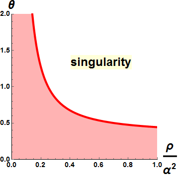
The DBI case (12) corresponding to $\Theta<0$ has been analyzed in depth in the literature and it corresponds to a metallic CFT [48]; the main novelty of our work refers to the iDBI (corresponding to $\Theta>0$) which gives rise to insulating CFTs.

As it is well known, the DBI case is protected by a symmetry, a non-linearly realized higher-dimensional Poincare group, see e.g. [49, 50]. For this reason, the DBI action admits a geometrical interpretation as a brane with a localized gauge field that is embedded in higher dimensional space. The brane realizes the spontaneous breaking of the higher-dimensional Poincare group down to the 3+1 dimensional one. The action then is fixed by this nonlinearly realized symmetry to the familiar Nambu-Goto form $\sim(q^{2}/\Theta){\rm Det}\Big({g_{\mu\nu}+\sqrt{-\Theta}F_{\mu\nu}}\Big)$ at leading order in the derivative expansion (which implies that the action depends also on $\tilde{F}_{\mu\nu}F^{\mu\nu}$, but we are ignoring this here). What we want to highlight now is that the iDBI case is also protected by the same symmetry, as it is quite obvious since the structure of the Lagrangian is the same. In the geometrical realization, the $\Theta>0$ case represents a brane with negative tension yet with a healthy gauge field embedded in it, which corresponds just to the continuation of (10) with $p=1/2$ to $\Theta>0$. The negative tension might raise concerns about the potential problems finding a UV completion of this action. Some of these concerns have been rather sharply articulated previously, e.g., in [51]: EFTs with higher order operators with the ‘wrong’ sign (such as what happens in the iDBI case) are argued to present generically super-luminal modes and therefore to lack a Lorentz invariant UV completion. Let us note only here that it is quite obvious that the UV completion of the low-energy effective scale-invariant field theory that captures strongly coupled materials is inevitably non-relativistic (at least in its first step, which must be phrased in terms of non-relativistic degrees of freedom – atoms). It is at present unclear to us whether or not the iDBI models have superluminal modes (see the Appendix A for some discussion). But even if there were, it is not clear either whether this is directly a problem. In the effective holographic models the light-cone structure of the gravity dual corresponds to an emergent light cone, which in realistic cases has a subluminal limiting velocity (such as what similarly happens in graphene). Therefore, we don’t find that this is an immediate logical obstacle that forces one to disregard the models of iDBI type, even though it is certainly an issue that deserves further study.

In any case, whether or not the choice of NED Lagrangian is protected by a symmetry (and whether or not it admits a Lorentz invariant UV completion) is a secondary issue for our analysis, so we will just continue with a generic $K$ and particularize for the two models (12) and show the results. In the sequel, we analyze the implications of introducing such non linearities in the context of the transport properties of the dual CFTs.

The DC conductivity for this model reads:

$$\boxed{\sigma_{DC}=K^{\prime}({\cal E}^{2}(u_{h}))+\frac{q^{2}\,\rho^{2}\,u_{h}^{2}}{M^{2}(u_{h})}}$$

(18)

where $M^{2}(u_{h})=m^{2}\,\alpha^{2}\,V^{\prime}(\alpha^{2}\,u_{h}^{2})$. The interested reader can find the derivation of this result in Appendix B. For future reference, we will define the first term in (18) as the ‘probe’ conductivity (see Eq. (31)),

$$\sigma_{P}=K^{\prime}({\cal E}^{2}(u_{h}))~.$$

For the benchmark models (12) along with the choice of a linear potential

$$V(z)=z/2m^{2}$$

for the $\phi$ scalars (so that the $\alpha$ parameter encodes the disorder strength), the DC conductivity reads:

$$\sigma_{DC}\,=\,\sqrt{1-\rho^{2}\,u_{h}^{4}\,\Theta}+\frac{2\,q^{2}\,\rho^{2}\,u_{h}^{2}}{\alpha^{2}}\,.$$

(19)

From this and (15), one can straightforwardly obtain how $\sigma_{DC}$ depends on $T$, $\rho$, etc. In this section we focus on the iDBI models (12) with full backreaction, since this gives rise to an insulating behaviour.

It is quite clear upon series expansion around $\rho=0$ that there is a very dramatic change of behaviour for (19) at $T=0$ above a certain threshold for the self-interaction parameter, specifically $\Theta>(2/3)q^{2}$ ⁹⁹ 9 This defines the second threshold mentioned above as $\Theta_{2}=2q^{2}/3$. . Above this threshold, the DC conductivity decreases with increasing $\rho$ (at constant $T$), a feature that is very far from the Drude metal. Instead, this is quite reminiscent of the traffic jam picture of a Mott insulator. Note that this threshold is larger than the threshold $\Theta>q^{2}/3$ that imposes an upper bound on the the charge density $\rho<\rho_{\star}$. The various different bahaviours of the electric conductivity (at zero temperature) that one can have depending $\Theta$ are summarized in Table 1 and in Figs. 3 and 4.

More specifically, for non-zero disorder strength $\alpha$ one can distinguish 4 cases:

• •

  $\Theta<q^{2}/3$ : there is no problem to satisfy $u_{h}<u_{\star}$ at any $T$ and $\rho$. The probe conductivity at $T=0$, $\sigma_{P}^{0}$, (31) is positive and less than 1 ( the Maxwell value in unit of $q^{2}$); the complete one at $T=0$, $\sigma_{DC}^{0}$ is positive too and getting larger and larger than 1 increasing the charge density $\rho$.

• •

  $q^{2}/3<\Theta<2\,q^{2}/3$ : for $\theta>q^{2}/3$ there is always a maximum density, $\rho_{\star}$, such that $u_{\star}=u_{0}$ and $\sigma_{P}^{0}=\chi^{0}=0$ (probe DC conductivity and charge susceptibility at zero temperature), with $\rho_{\star}$ given in (17). The full DC conductivity (given by (19)) at this particular value of the charge density and at zero temperature reads:

  $$\sigma_{DC\star}^{0}=\frac{q^{2}}{3\,\theta-q^{2}}$$

  (20)

  and it is surprisingly independent of the disorder strength $\alpha$. In this regime, $\sigma^{0}_{DC}$ satisfies $\partial\sigma^{0}_{DC}/\partial\rho>0$ (no traffic jam). At $\rho_{\star}$, this is larger than 1, but bounded.

• •

  $\Theta=2\,q^{2}/3$ : At $\rho_{\star}$ we have $\sigma_{P}^{0}=0$ while $\sigma^{0}=1$ (in units of $q^{2}$) for every $\rho_{\star}$.

• •

  $\Theta\geq 2\,q^{2}/3$ : At $\rho_{\star}$ we have again $\sigma_{P}^{0}=0$. Now, though, there is ‘traffic jam’, $\partial\sigma_{DC}^{0}/\partial\rho<0$. The value of $\sigma_{DC}^{0}$ at the maximum density $\rho_{\star}$ goes like $q^{2}/(3\,\Theta)$ for large $\Theta$ and can be therefore arbitrarily low.

We now turn to the study of the ‘optical’ AC conductivity for the iDBI model in different setups and we will come back to the $T=0$ features in the next section 3.2. For the rest of the paper we fix $q=1$ unless explicitly stated.

The first case we present is the linear metric potential case $V(z)=z$ (the model of [9]), which in the absence of non linear electronic interactions has metallic behaviour. On top of this background we switch on the iDBI non-linearities in the electron sector which results in a suppression of the DC conductivity. The results are shown in Fig. 5 for some representative parameters.

The iDBI case with $V(z)=z$ already shows quite remarkable features:

• •

  It suppresses the DC conductivity, leading to insulating behaviour at low T.

• •

  The competition between the linear potential for the bulk phonons $\phi$ and the non linear iDBI for the electrons produces already a metal-insulator crossover upon dialing the temperature of the geometry.

• •

  A pinned response in the optical conductivity appears – it is entirely due to the electron sector. For small $T$, we notice the appearance of a rather broad but certainly visible resonance at nonzero frequencies. This resonance becomes narrower for bigger $\Theta$ and/or $\rho$ closer to $\rho_{\star}$. Given the interpretation that we are proposing here as traffic-jam-like behaviour, it is natural to interpret this resonance as an accordion wave effect.

• •

  Even at temperatures where the Drude peak is present it seems that also additional features appear at higher-frequencies.

One can of course complicate the situation considering also non linear potential in the bulk phonons sector. One interesting case is for example to take the potential of [10]. The results for the iDBI model with non linear potential $V(z)=z+z^{5}$ are shown in figure 6, and can be summarized as:

• •

  The DC conductivity at low temperature is considerably reduced, thus realizing a rather good insulator ($\sigma_{DC}(T=0)\ll 1$) and keeping the metal-insulator crossover already present in the model at finite $T$.

• •

  The mid-infrared peak observed in [10] is still present in the optical conductivity and it seems to be enhanced by the iDBI non linear extension, meaning that electron-electron interactions can contribute to sharpen that resonance.

  Since in this case the resonance is also present at $\Theta=0$, this resonance represents a polaron [10] which, at $\Theta\neq 0$, also includes charge-sector nonlinearities.

• •

  The iDBI non linear interactions provide a second mild peak for larger frequencies which was not present in [10]. It would be interesting to understand further the nature of that peak in relation to the pinned response of real Mott Insulators.

The next interesting question is: can we find out a model where the non-linearities in the electronic sector (e-e interactions) provide a metal-insulator transition? Is there a tunable parameter we can dial to drive a MIT? In other words, can one find a Quantum Phase transition where the two phases (metallic and insulating) are connected dialing an external parameter while keeping the temperature to be zero?

It is then necessary and interesting to find out a tunable parameter whose dialing can induce such a mechanism. Taking into account that the iDBI corresponds to an insulator while the DBI to a metal, it quite obvious that that the parameter connecting those models in a continuous way is none other than the $\Theta$ parameter that controls the strength (and sign) of the e-e interactions in the benchmark models (12). Fixing the charge density and the disorder strentgh (i.e. graviton mass) and dialing the $\Theta$ parameter we can indeed provide in the full backreacted model a nice metal-insulator transition which is clearly driven just by the electronic sector’s non linearities (that is, e-e interactions) and it represents a holographic simple toy example of the so called Mott transition. An example of this result (making use of formulas (19)) is shown in fig.7.

As expected, we can interpolate between the metallic and the insulating behaviour dialing $\Theta$, that is, by changing the non-linear terms in the field strength $F_{\mu\nu}$. We can indeed focus on the $T\approx 0$ value of the DC and see how this goes from a finite (i.e. $\sigma>1$) value to a small and eventually $\approx 0$ one dialing $\Theta$. $\Theta=0$ corresponds to the Maxwell case; once we start increasing the value of $\Theta$ we depart from the Maxwell case and depending if we go towards negative or positive values we run into a metallic or an insulating phase.

From the technical point of view the extremality condition (once fixed the amount of charged density $\rho$ and the disorder strength, i.e. the graviton mass, in an safe way following fig.2) fixes a maximum value for $\Theta=\Theta_{0}$. The DC conductivity at that value can be computed analytically from the expression (19). Depending on the value of $\rho$ and $\alpha$ the DC value at $T=0$ (namely at $\Theta=\Theta_{0}$) can become arbitrarily small (but exactly zero just at $\rho=\rho^{\star}$ and $\Theta=\infty$, see table 1).
This certainly requires a certain tuning of parameters¹⁰¹⁰ 10 The notion of tuning in condensed matter is slightly different than in particle physics. Most of the High $T_{c}$ superconductors are synthetic compounds that present significant amounts of design, and therefore can be considered as tuned systems., as we did in the example of Fig.7. To make things clearer we also plot the value of the DC conductivity at zero temperature in Fig.8, with the same parameters of Fig.7.

Let us emphasize is that at this level, there is no direct link of the $\Theta$ parameter into external control parameters that can be used in real condensed matter, and this question is beyond the scope of this article. One clear statement, though, is that $\Theta$ clearly has to do with the amount (and sign) of non-linearities in the Maxwell sector. Dialing $\Theta$, then, must correspond to increasing/decreasing the strength of electron self-interactions and consequently their mobility. We expect the iDBI case to mimic some sort of strong coulomb interaction between electrons which leads to pinning behaviour à la Mott. Definitely, it would be illuminating to understand better its role and search for a better parameter to dial to compare with real situations.

Let us also mention that these results also imply that same model also exhibits MITs (at fixed $\Theta$) by varying various other external parameters such as $\mu$, $\rho$ or $T$, at least in some region of the parameter space (and with the conductivity decreasing in the insulating phase to a finite but small value).

From the non-linear nature of the charge sector of these models, it it clear that a very generic property of these models is that they should display a strong nonlinear response. Let us initiate here the analysis of the nonlinear response by studying the simplest in principle observable, namely, the static charge susceptibility. See also [52] for similar analyses in the holographic context.
The solution for the gauge field in the general model reads:

$$A_{t}(u)\,=\,\int_{u}^{u_{h}}\frac{{\cal E}(t)}{t^{2}}\,dt$$

(21)

and already implements the regularity condition at the horizon. From (21) we can define the chemical potential and the charge density for instance as

$\displaystyle\mu\,=\,A_{t}(0)-A_{t}(u_{h})\,,\,\,\,\,\,\,\,\,\rho\,=\,-A_{t}^{\prime}(0)\,,$

(22)

which is as much as requiring the gauge field to asymptote close to the boundary to $A_{t}=\mu-\rho\,u$. For the Maxwell theory the solution reads ${\cal E}(u)=\rho\,u^{2}$ such that we recover the usual expression $\mu=\rho\,u_{h}$. Consequently, the static charge susceptibility (at constant entropy density $s\,=\,2\pi/u_{h}^{2}$)

$$\chi_{E}\,=\frac{\partial\rho}{\partial\mu}$$

is just equal to $u_{h}^{-1}$. Instead, in the non-linear models (12) the relation between chemical potential and charge density instead is easily seen to be given by

$$\mu\,=\,\rho\,u_{h}\;{}_{2}F_{1}\left(\frac{1}{4},\frac{1}{2};\frac{5}{4};u_{h}^{4}\,\rho^{2}\,\Theta\right)~,$$

(23)

where ${}_{2}F_{1}\left(a,b;c;z\right)$ is the hypergeometric function. Again we see that at large temperature, which corresponds to small $u_{h}$, these theories are just a small deformation around the linear Maxwell theory:

$$\mu\,=\,\rho\,u_{h}\,+\,\Theta\,\frac{\rho^{3}\,u_{h}^{5}}{10}+O\left(u_{h}^{6}\right)+\dots$$

(24)

An example of susceptibility in function of temperature (at constant charge density) and of the $\rho-\mu$ curve at constant entropy density is shown in figure 9 for different $\Theta$ and zero momentum dissipation.

One can see the two different effects induced by the non linear (12) models are sensitive just in the range of large $u_{h}$ (small $T$), as expected. While the DBI model enhances the response of the charge density to a chemical potential, the iDBI decreases it. More about this quantity is shown in fig.10 where the plots are generalized for finite momentum dissipation and at constant temperature T.

The common feature is that at $\rho=\rho^{\star}$ (and at $\Theta=q^{2}/3$ for zero momentum dissipation) the charge susceptibility $\chi$ is zero at zero temperature and this correlates with the vanishing of the probe conductivity. As already shown in fig.2 for $\Theta>q^{2}/3$ there is a maximum amount of charge density $\rho^{\star}$ (and of relative chemical potential $\mu^{\star}$) which the system can afford, while for $\Theta<q^{2}/3$ there is no such a bound as shown in fig.10.

The equation for a probe vector on top of our geometry (with unspecified $f(u)$) at zero momentum reads:

$$\frac{{\cal E}(u)}{u^{2}}\partial_{u}\left(\frac{u^{2}\,f(u)}{{\cal E}(u)}a^{\prime}(u)\right)+\frac{\omega^{2}}{f(u)}a(u)\,=\,0$$

(30)

In this approximation the DC conductivity is just:

$$\sigma_{DC}^{P}=K^{\prime}({\cal E}^{2}(u_{h}))$$

(31)

As expected in the case of the linear theory (i.e. Maxwell), this quantity is trivially constant and it coincides with the conformal value 1.

We want to study the model (12) and its transport properties; we are particularly interested in the case iDBI cases (12) where the dual CFT exhibits insulating behaviour¹²¹² 12 The DBI case has been extensively studied previously – it shows purely metallic nehaviour [48].. The DC conductivity takes the simple form

$$\sigma_{DC}^{P}\,=\,\sqrt{1-\rho^{2}\,u_{h}^{4}\,\Theta}~.$$

(32)

To discuss the temperature dependence of this one needs to assume something for $f(u)$, and how it is affected by the chemical potential. We start considering the non linearly charged BH geometry with zero momentum dissipation, $\alpha=0$, (probe limit II); we emphasize that in that case we necessitate $\Theta\leq(q\ell)^{2}/3$ to have a well defined extremal black hole. From now on, we set $q\ell=1$. One important feature that determines the nature of the dual CFT is the DC conductivity at zero temperature which within this easy approximation can be computed directly and reads:

$$\sigma_{DC}^{0}\,=\,1-\,3\,\Theta$$

(33)

It is nice to see that there is another clear indication that the model for $\Theta>1/3$ is not safe in the probe limit which is encoded in the fact that the DC conductivity becomes negative.

This formula explicitly shows how for $\Theta\leq 1/3$ the DC value is always less than the linear Maxwell case, which tells us that the iDBI choice (12) somehow obstructs the charge carriers’ mobility, leading to an insulating behaviour.

One also notices that in the limit where $\Theta$ is very close to the maximum value $1/3$ and the corresponding “material” is a very good insulator a peak in the optical conductivity appears and gets sharper, see Fig. 12. An important point to underline is that the optical conductivity (in the probe limit as in the rest of the paper) shows a soft-gapped behaviour, while real Mott-Insulators are defined by an hard-gapped one¹³¹³ 13 It has been recently argued that in ‘many body localized systems’ there could exist a power law $\sigma(\omega)\propto\omega^{\beta}$ behaviour at low frequency with $1<\beta<2$ [56]. It would be nice to check and study further this scaling in our class of models.. Within the present holographic models it appears very difficult to produce such hard gap. To reproduce this feature, it seems that one needs to resort to a dilaton with nontrivial running.

We then go to the ‘probe limit I’, where the background is completely dictated by the momentum dissipation sector, $\alpha\neq 0$. Doing so in order to have a well defined extremal limit for our black hole we need to satisfy the bounds explained before and summarized in Fig. 2. We emphasize that from now on, wherever not explicitly said, we are using the choice (12) with $\Theta=1$.

Figure 13 shows that the non-linear extensions of Maxwell theory modify the DC conductivity (even in the probe vector limit), which now acquires a non trivial temperature dependence. At large temperature we recover the usual Maxwell (constant) result, as it should because large $T$ corresponds to small $F^{2}$ and we are considering only choices of $K(z)$ that go linear $K(z)\simeq z+\dots$ at small $z$. The low temperature behaviour, on the contrary, is very sensitive to the non-linearities and the particular model considered.

The iDBI (12) shows a strong suppresssion of the DC conductivity towards small temperatures and eventually a vanishing DC conductivity at $T=0$ can be obtained (by dialing $\Theta$ and/or $\mu$). This is the main reason to interpret these models as insulators. In a sense, in the iDBI models the electronic interactions are such that the charge carriers conductance is suppressed at small temperature. Conversely, the usual DBI model increases the DC conductivity at small T exhibiting a typical metallic behaviour [48].

We continue with the analysis of the optical conductivity for the choice (12): the results are plotted in figures 14 and 15.

In all the cases the large frequency limit coincides with the usual Maxwell conformal case (which in $2+1$ dimensions acquires the constant value $\sigma_{\infty}=1$); this is again a direct consequence of the fact that non linearities are relevant just in the IR region of the geometry while they dont affect any UV property.

The DBI model exhibits at small temperatures a clear Drude Peak behaviour which is characteristic of metallic materials; decreasing the temperature a smooth crossover drives into an incoherent metallic phase where the AC conductivity is almost constant and no dominating excitation appears. One can easily keep track of this dynamical behaviour studying the motion of the quasinormal modes of the system with temperature as done for a different setup in [58].

The iDBI provides for a completely different phenomenology: there is a strong suppression of the conductivity at small frequencies and a spectral weight transfer to a ‘mid-infrared’ peak. These features classify this model as an insulator. In this case the QNMs spectrum would be more similar to the one shown in [10].
Note that in this section (5) the metric fluctuations are switched off and therefore we lack of a stress tensor in our CFT, this is the reason why we dont see any infinite in the DC conductivity and the reason why we do not need any dissipative mechanism to enter in the game. All the properties in this section just arise from the electron-electron interactions provided by the non-linear electromagnetic extension (although the thermodynamics, at least in the second approximation, is also affected by the dissipative sector).

Let us now discuss the non-linear electrical response. The standard way to describe it is by exhibiting the nonlinear current-voltage ($J-E$) diagram, which encodes a nonlinear version of the electrical conductivity. We shall restrict to the DC case and to the simplest but nontrivial case to analyze, namely the probe vector limit where we neglect any mixing with the vector modes in the metric but still we keep all the nonlinear self-couplings of the gauge field. Similar studies have been done before, see [53, 54, 55].

We introduce an ansatz for the gauge field $A_{t}=A_{t}(u)$ and $A_{x}=E_{x}\,t+\delta A_{x}(u)$¹⁴¹⁴ 14 Note that this ansatz differs from the one in [53, 54] in that we are including the ‘backreaction’ of $\delta A_{x}(u)$ on $A_{t}$, which can be non-trivial starting at order $E^{2}$ for non-canonical kinetic terms. This suggests that at nonlinear level the $\mu-\rho$ curve also depends on $E^{2}$, but we shall not discuss this effect here.. The NED-Maxwell equations in a black brane background with a generic emblackening factor $f(u)$ reduce to

	$\displaystyle K^{\prime}\left({-F^{2}\over 2}\right)\,A_{t}^{\prime}=-\rho$		(34)
	$\displaystyle K^{\prime}\left({-F^{2}\over 2}\right)\,f(u)\,\delta A_{x}^{\prime}=J_{x}\$		(35)

where (since $K^{\prime}(0)=1$) we already identified the integration constants $\rho$ and $J_{x}$ as the charge density and charge current. The field-strength invariant reduces to

$$z\equiv{-F^{2}\over 2}=u^{4}\left(A_{t}^{\prime 2}+{E_{x}^{2}\over f(u)}-f(u)\delta A_{x}^{\prime 2}\right)$$

(36)

Using (34) and demanding $z$ to be regular at the horizon, one quickly obtains that

$$J_{x}=K^{\prime}\left({-F^{2}\over 2}\right)\Big|_{u_{h}}\;E_{x}$$

(37)

which nicely reproduces the linear conductivity result for small fields.

However, (37) is much more informative now, as it holds for any value of $E_{x}$ and, indeed, $K^{\prime}|_{u_{h}}$ depends nonlinearly on $E_{x}^{2}$. Let us make this dependence more manifest.

To illustrate this, let us turn to the DBI/iDBI cases, the computation simplifies a lot. The equations of motion (34) can be brought to the form

$$-{A_{t}^{\prime}\over\rho}={f(u)\delta A_{x}^{\prime}\over J_{x}}=\sqrt{\Theta\,E_{x}^{2}\,u^{4}+f(u)\over\Theta\,J_{x}^{2}\,u^{4}+(1-\Theta\rho^{2}u^{4})\,f(u)}$$

(38)

There is a choice of integration constants that maximizes the regularity of the solution, namely, that the argument of the square-root does not change sign anywhere. This could happen at the point $u_{c}=u_{c}(E_{x}^{2})$ defined by

$${f(u_{c})}+\Theta\,u_{c}^{4}\;E_{x}^{2}=0~.$$

(39)

At the same point one must then require

$$J_{x}^{2}\,u_{c}^{4}+(1-\Theta\rho^{2}u_{c}^{4})\,f(u_{c})=0$$

so that the nonlinear conductivity is

$$\sigma_{NL}\equiv{J_{x}\over E_{x}}=\sqrt{1-\Theta\,\rho^{2}\,u_{c}^{4}}~.$$

(40)

It is easy to check that this indeed coincides with $K^{\prime}|_{u_{h}}$.

Note that for DBI models, $u_{c}<u_{h}$ whereas for iDBI models $u_{c}>u_{h}$. The IR regularity condition in that case originates from behind the horizon, which is certainly a bit intriguing. However, we do not find this to be necessarily a problem from any practical point of view (see Appendix C for more details about it).

We summarize in Fig. 16 the resulting nonlinear $J$-$E$ diagram. For DBI models, one clearly sees that at large $E$ one recovers $\sigma_{NL}=1+O(E^{-2})$. Therefore, even if the $J-E$ curve is entirely above the $J=E$ line, the nonlinear effect is to reduce the conductivity (from $\sqrt{1-\Theta\rho^{2}u_{h}^{4}}$ to $1$). This is welcome since the Coulomb e-e interactions are expected if anything to reduce the conductivity. And as we see this does happen at high field even for the DBI case (which is the one where the linear conductivity is enhanced with respect to the Maxwell case).

For the iDBI models the nonlinear effect is also to reduce the conductivity, but in a more dramatic way. Indeed, $\sigma_{NL}$ vanishes at some finite $E_{x}$. There is both a maximum current and voltage (or applied field $E_{x}$) that the material can withstand. Presumably, the region where the $dJ/dE<0$ signals an instability, akin to the electrical breakdown of insulators. The details of this instability are left for future investigation.

One also notices in Fig. 16 that the curves terminate at a maximal applied field $E_{x}$ in a branch-point fashion. This suggests that at that point one the gauge field becomes complex and therefore a naked singularity should re-appear. For such large applied voltage, then, one needs to do a proper analysis by including the backreaction. We defer this to future work.

Interestingly enough, nonlinear current-voltage curves quite close to the ones for the iDBI models have been measured in some lanthanide and cuprate compounds, [69]. See also [70, 71] for other studies of the nonlinear electric response in strange metals.