Ferromagnetism and d+id superconductivity in 1/2 doped correlated systems on triangular lattice
Abstract
We investigate the quantum phase diagram of t-J model on triangular lattice at 1/2 doping with various lattice sizes by using a combination of density matrix renormalization group (DMRG), variational Monte Carlo and quantum field theories. To sharply distinguish different phases, we calculated the symmetry quantum numbers of the ground state wave functions, and the results are further confirmed by studying correlation functions. Our results show there is a first order phase transition from ferromagnetism to d+id superconductivity, with the transition taking place at .
pacs
Valid PACS appear hereI Introduction
The triangular lattice is the building block of many transition metal oxides [1, 2, 3, 4] and organic salts [5, 6, 7, 8], in which it adds geometric frustration to the interacting electrons. Correlated electronic systems on the triangular lattice have attracted considerable attention[9, 10], and interesting quantum phases have been revealed in a number of materials including unconventional superconductivity [11, 12] and quantum spin liquids [13, 14].
It remains challenging to theoretically understand the quantum phase diagram of such correlated electronic systems, in particular in the presence of doping. It is nevertheless known that the interplay between different competing orders, e.g., superconductivity and magnetism, could play a crucial role [15].
In this work we consider the t-J model on the triangular lattice, which has been an especially useful model to describe many transition metal oxides:
| (1) | ||||
Here is the Gutzwiller projection that projects out the double occupancies in t-J model, labels the annihilation operator, denotes the spin index, and label the spin and density operators on site respectively. We will consider particular commensurate fillings, corresponding to () electrons per site for the positive (negative) nearest neighbor hopping amplitude . Since these two cases are related by a particle-hole transformation and thus can be treated simultaneously, below we focus on the positive case.

At this particular filling, the Fermi surface of the non-interacting nearest neighbor tight-binding model has two obvious features: as shown in Fig.1, the hexagon shaped Fermi surface is nested by three nesting wavevectors , and has three van Hove singularities located at M-points .
Such a Fermi surface is clearly unstable even in the presence of weak interactions. A conventional mean-field analysis leads to spin-density-wave(SDW) orders at the nesting wavevector [16]. Among different kinds of SDW orders, a particularly interesting pattern is the so-called chiral SDW (c-SDW) which features quantized anomalous Hall effect [16, 17]. In addition, a recent renormalization group analysis shows that, at least for weak interactions, the ground state of the system should be a chiral d+id superconductor (SC) due to the scattering processes involving the van Hove singularities [18].
However, the t-J model has no weak coupling limit, so it is unclear whether the weak coupling results apply, although they highlight the competition between superconductivity and magnetism in the 1/2 doped triangular lattice system. In addition, in the strongly coupled, small regime, (adiabatically connected to the large regime of the Hubbard model), it has been argued that ferromagnetism is an important competing phase at least when the doping is small [19]. This motivates us to carefully study the quantum phase diagram of the t-J model in this system.
In order to quantitatively investigate the quantum phase diagram of such a strongly correlated system, we use intensive numerical simulations which can provide the ground states without bias. However, reliably distinguishing competing quantum phases in such simulations has been a long-standing theoretical challenge. This is mainly due to the following conflict. On the one hand, numerical simulations become prohibitively demanding as system size grows. On the other hand, quantum phases are generally defined by their long-range physics, which requires measuring long-range correlation functions. But does one always need long-range physics to distinguish candidate quantum phases? The answer is no, and we take advantage of this fact.
As a trivial example, in order to distinguish a ferromagnetic phase and the spin-singlet superconductor phase, instead of measuring long-range correlators, one could simply look at the ground state spin quantum numbers even on rather small samples. The ferromagnetic phase should feature a large spin quantum number while the spin-singlet superconductor wave function should be in the spin-singlet sector. In more complicated examples, candidate quantum phases may have distinct lattice quantum numbers, which are generally nontrivial to compute yet are accessible numerically.
When two quantum phases are found to host distinct quantum numbers (lattice, spin, or other quantum numbers) on a sequence of finite size samples up to the thermodynamic limit, they are distinct in their short-range physics. We distinguish quantum phases in numerical simulations by comparing quantum numbers in a sequence of smaller system sizes, without having to perform the challenging finite size scaling of correlators in larger system sizes.
In this work, we study the phase diagram of the model systems using a combination of analytical construction of symmetric wave functions, the density matrix renormalization group(DMRG) [20, 21, 22, 23] and the variational Monte Carlo numerical simulations [24, 25, 26, 27]. DMRG has been shown to be a nearly unbiased numerical simulation method and has been successfully applied to strongly correlated electronic systems [28, 29]. The basic strategy of our method is first analytically studying the characteristic symmetry quantum numbers of candidate quantum phases, and then comparing them with numerical ground state wave functions obtained from DMRG. This allows us to distinguish the candidate phases reliably even on limited system sizes. The phase diagram is then further confirmed based on correlation function measurements and a complementary variational Monte Carlo study. Previously, this method has been successfully applied to quarter doped correlated electronic systems on the honeycomb lattice [28].
We perform DMRG simulations on 16-sites, 28-sites, and 36-sites samples, which are shown in Fig.2.

Our calculation reveals that for , the system develops ferromagnetism, while with increasing J a first order phase transition into a d+id superconductor occurs. The main results are summarized in Fig.2(c).
This paper is organized as follows. In Sec. II, we construct the wave functions of c-SDW and d+id SC, and calculate the relevant symmetry quantum numbers for various system sizes, analytically and using variational Monte Carlo simulations. In Sec.III we compare these results with DMRG analysis, including spin-spin and pair-pair correlations, to justify the phase diagram in Fig.2(c).
II Wave functions of c-SDW and d+id SC
We first construct the c-SDW wave functions using the slave-fermion approach [30, 31, 32, 33, 34], where we rewrite the electron annihilation operator as bosonic spinons and fermionic spinless holons:
| (2) |
Rewriting the t-J Hamiltonian Eq.(1) into spinons and holons, the Hamiltonian can be split into two parts at the mean field level: the bosonic part, which describes a bosonic superconductor, and the fermionic part, describing a charge Chern insulator:
| (3) |
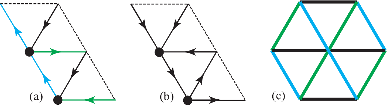
where and are the boson singlet hopping and pairing parameters on bond ij, is the spinless fermion hopping parameter, and are the boson and fermion chemical potential respectively. By gluing the wave functions from these two Hamiltonians, one can obtain the wave function describing the whole Hamiltonian. Changing parameters , , and , and following the projective symmetry group (PSG) [35, 36, 37] analysis (see Appendix B), we find the real space pattern of , and that describes the c-SDW phase, as depicted in Fig.3(a) and Fig.3(b). Analogous states with doubled unit cells are called flux states in quantum spin liquids.
The construction of the wave function that describes d+id SC is simpler: we use the slave boson approach [35, 36], where the electron is split into fermionic spinon and bosonic holon:
| (4) |
If the fermionic spinons form a d+id band structure while the bosons are condensed at point of the Brillouin Zone, then the system gives a d+id superconductor, and the mean field Hamiltonian can be written as:
| (5) |
where is the hopping parameter, are the pairing parameters. The parity of the SC is determined by the symmetry of the pairing parameters. To accommodate d+id SC, we set the relative phases of , as depicted in Fig.3(c), with bonds of different directions being , and .
III Numerical Simulations
To sharply distinguish candidate phases on finite size samples, we analytically computed the symmetry quantum numbers of c-SDW and d+id SC states which are further confirmed by variational Monte Carlo numerics. Let be the many-body state, and be the symmetry operator, then is the transformed state and is the corresponding many-body quantum number. This quantum number can be computed by taking the ratio: , where is state labeled by a real space spin and hole configuration.
We focus on symmetry operators , , and inversion(i.e. ), where is the lattice translation along and is the rotation, as shown in Fig.4. As listed in Table 1, we computed the ground state quantum numbers of c-SDW and d+id SC on various samples. Between the 16-sites and 36-sites samples (see Fig.2(a)) all the considered symmetry quantum numbers are identical, preventing us from distinguishing c-SDW and d+id SC. However, the chosen 28-sites hexagonal sample (see Fig.2(b)) is suitable to sharply distinguish these phases. Note that the d+id SC (or c-SDW) phase breaks the time-reversal symmetry and one can construct two wave functions that are time-reversal images of each other. When quantum numbers are different for these two wave functions, they will form a two-fold irreducible representation of the global symmetry.


| Symmetry | c-SDW or d+id SC |
|---|---|
| Inversion |
(a) 16 or 36 sites sample.
| Symmetry | c-SDW | d+id SC |
|---|---|---|
| Inversion |
(b) 28 sites sample.
| 0.6 | 0.001783 | 0.001287 | 0.001837 | -0.277946 | 0.286516 |
| 0.8 | 0.003922 | 0.002356 | 0.002044 | -0.268602 | 0.340033 |
| 1.0 | 0.003117 | 0.002885 | 0.002801 | -0.354765 | 0.328343 |
| 1.2 | 0.004177 | 0.003216 | 0.003289 | -0.344315 | 0.347355 |
| 1.4 | 0.005628 | 0.004387 | 0.004712 | -0.347967 | 0.358649 |
| 1.6 | 0.008756 | 0.006370 | 0.006951 | -0.348524 | 0.371596 |
| 1.8 | 0.013474 | 0.010153 | 0.009597 | -0.369925 | 0.352528 |
| 2.0 | 0.017143 | 0.012216 | 0.011950 | -0.367776 | 0.366071 |
We perform DMRG simulations for the three samples in Fig.2. First, the ground state energy has already provided useful information, see Fig.5. For 16-sites sample, there is a horizontal plateau in the region of whose energy stays at -1. This is a signature of the ferromagnetic order. Because with spin-polarized electrons, the J term in t-J model vanishes and the ground state energy can be computed based on the non-interacting hopping problem. On this sample, by filling all the 8 electrons in the spin-polarized band, one finds the energy per site to be . For the 36-sites sample with 18 electrons, the situation can be understood as follows. We label the sectors by the total spin quantum number. There are 10 non-negative sectors ranging from 0 to 9, with being fully polarized along the -direction. The fully polarized ferromagnetic state still produces , but it is not the ground state. Instead, the ground states are found to form a total spin representation and one of them is in the sector, producing an energy curve with a slight slope as indicated by the blue curve in Fig.5. We believe that this result is a consequence of the specific energy shell structure on this sample: Let us denote the majority spin flavor to be spin up, then 17 spin-up electrons would fully fill the energy shell for the spinless hopping Hamiltonian (Fig.4(b)), leaving one extra down spin. It is reasonable to expect that this is a finite size artifact and the fully polarized ferromagnetism would be restored in the thermodynamic limit.
To understand the nature of the phase with large , we calculate the symmetry quantum numbers of the DMRG ground states. We find , and for the ground states in this regime on all the three samples, which is consistent with both candidate phases (see Table 1). However, the quantum number of DMRG ground state on the 28-sites sample can be used to sharply distinguish the phases, and we find it to be consistent with the d+id SC phase. Technically, here we take advantage of the fact that the model Hamiltonian is purely real (in the real-space spin configuration basis). Consequently the DMRG simulation gives a purely real ground state wave function . If the ground states of the model form a two-fold irreducible representation as the d+id SC on the 28-sites sample(see Table 1), then the DMRG wave function would be an equal weight superposition of the and states, and the expectation value of the transformation operator: would be . On the other hand, this expectation value would be for the c-SDW state. We have measured this expectation value in the large regime using the standard Monte Carlo technique(see Fig.6), and the result is clearly consistent with . (Here we have projected the to the center of momentum point for better convergence.)


Next we confirm the nature of the DMRG ground state in two more ways: (1) The energy of the d+id SC trial wave function proposed in Section II is calculated using the variational Monte Carlo technique[25] and compared to the DMRG ground state. As can be seen in Fig.7, the optimal d+id SC wave function obtained by tuning only one variational parameter (the nearest neighbor pairing) can already produce of the energy of DMRG ground state energy. (2) The pair-pair correlation function of the DMRG ground state are measured, as shown Table 2. One key signature of the d+id pairing is the relative phase of the pairing on the real space bonds, as depicted in Fig.3(c). We calculated the pair-pair correlation function, defined as , where is the singlet pairing, while and are two nearest neighbor sites forming a bond. The bonds are chosen with farthest distance in the sample, with fixed and in three options varied by directions, as shown in Fig.2(b). We find that the pattern of the relative pairing phases is consistent with the d+id SC.
IV Discussion and Conclusion
Based on the idea of using quantum numbers in finite system sizes to sharply distinguish candidate quantum phases, we investigate the quantum phase diagram of the t-J model on the triangular lattice at 1/2 doping. As shown in Fig.2, ferromagnetic phase is realized in the the small regime, separated from a chiral d+id superconductor phase in the large regime.
The crucial advantage of the method adopted here is the capability to sharply distinguish candidate quantum phases even on small to intermediate size samples. To achieve this goal, we purposely choose samples so that candidate quantum phases have distinct quantum numbers. For instance, the c-SDW phase and the d+id superconductor share the same quantum numbers on the 36-sites sample, but feature different lattice quantum numbers on the 28-sites sample. Such analytical understanding of the symmetry properties provides important guidance in our numerical simulations.
One may wonder about the generality of this method. Indeed, in this study, we are fortunate to be able to only focus on a small number of candidate quantum phases, based on the special shape of the non-interacting Fermi surface and previous weak coupling analysis [18]. But in a general model, in principle one needs to take into account a large number of candidate phases and the present treatment scheme may become intractable. In this regard, hopefully one could develop a theoretical method to systematically diagnose symmetry properties of the quantum wave functions of candidate phases. A recent work based on tensor-network formulation is an attempt to develop such a general method [38].
This work is supported by Alfred P. Sloan fellowship and National Science Foundation under Grant No. DMR-1151440.
References
- [1] Q.-H. Wang, D.-H. Lee, and P. A. Lee, Phys. Rev. B 69, 092504 (2004).
- [2] A. Ralko, J. Merino, and S. Fratini, Phys. Rev. B 91, 165139 (2015).
- [3] M. Becker, M. Hermanns, B. Bauer, M. Garst, and S. Trebst, Phys. Rev. B 91, 155135 (2015).
- [4] H. F. Pen, J. van den Brink, D. I. Khomskii, and G. A. Sawatzky, Phys. Rev. Lett. 78, 1323 (1997).
- [5] Y. Shimizu, K. Miyagawa, K. Kanoda, M. Maesato, and G. Saito, Phys. Rev. Lett. 91, 107001 (2003).
- [6] T. Itou, A. Oyamada, S. Maegawa, M. Tamura, and R. Kato, Phys. Rev. B 77, 104413 (2008).
- [7] S. Yamashita, Y. Nakazawa, M. Oguni, Y. Oshima, H. Nojiri, Y. Shimizu, K. Miyagawa, and K. Kanoda, Nat Phys 4, 459 (2008).
- [8] H. Kino and H. Kontani, Journal of the Physical Society of Japan 67, 3691 (1998).
- [9] T. Kimura, J. C. Lashley, and A. P. Ramirez, Phys. Rev. B 73, 220401 (2006).
- [10] C. H. Chung, J. B. Marston, and R. H. McKenzie, Journal of Physics: Condensed Matter 13, 5159 (2001).
- [11] R. Schaak, T. Klimczuk, M. L. Foo, and R. J. Cava, Nature 424, 527 (2003).
- [12] B. Kumar and B. S. Shastry, Phys. Rev. B 68, 104508 (2003).
- [13] Y. Li, G. Chen, W. Tong, L. Pi, J. Liu, Z. Yang, X. Wang, and Q. Zhang, Phys. Rev. Lett. 115, 167203 (2015).
- [14] M. Yamashita, N. Nakata, Y. Kasahara, T. Sasaki, N. Yoneyama, N. Kobayashi, S. Fujimoto, T. Shibauchi, and Y. Matsuda, Nat Phys 5, 44 (2009).
- [15] H. Eisaki, H. Takagi, R. J. Cava, B. Batlogg, J. J. Krajewski, W. F. Peck, K. Mizuhashi, J. O. Lee, and S. Uchida, Phys. Rev. B 50, 647 (1994).
- [16] K. Jiang, Y. Zhang, S. Zhou, and Z. Wang, Phys. Rev. Lett. 114, 216402 (2015).
- [17] I. Martin and C. D. Batista, Phys. Rev. Lett. 101, 156402 (2008).
- [18] R. Nandkishore, R. Thomale, and A. V. Chubukov, Phys. Rev. B 89, 144501 (2014).
- [19] Y. Nagaoka, Phys. Rev. 147, 392 (1966).
- [20] U. Schollwöck, Rev. Mod. Phys. 77, 259 (2005).
- [21] U. Schollwöck, Annals of Physics 326, 96 (2011).
- [22] S. R. White, Physical Review Letters 69, 2863 (1992).
- [23] K. A. Hallberg, Advances in Physics 55, 477 (2006).
- [24] W. Foulkes, L. Mitas, R. Needs, and G. Rajagopal, Reviews of Modern Physics 73, 33 (2001).
- [25] C. Gros, Annals of Physics 189, 53 (1989).
- [26] D. Ceperley, G. V. Chester, and M. H. Kalos, Phys. Rev. B 16, 3081 (1977).
- [27] A. Harju, B. Barbiellini, S. Siljamäki, R. M. Nieminen, and G. Ortiz, Phys. Rev. Lett. 79, 1173 (1997).
- [28] S. Jiang, A. Mesaros, and Y. Ran, Physical Review X 4, 031040 (2014).
- [29] E. Jeckelmann and S. R. White, Phys. Rev. B 57, 6376 (1998).
- [30] F. Wang and A. Vishwanath, Phys. Rev. B 74, 174423 (2006).
- [31] S. Sachdev, Phys. Rev. B 45, 12377 (1992).
- [32] S. Sachdev and N. Read, International Journal of Modern Physics B 05, 219 (1991).
- [33] N. Read and S. Sachdev, Phys. Rev. Lett. 66, 1773 (1991).
- [34] D. P. Arovas and A. Auerbach, Phys. Rev. B 38, 316 (1988).
- [35] X.-G. Wen, Phys. Rev. B 65, 165113 (2002a).
- [36] X.-G. Wen, Physics Letters A 300, 175 (2002b), ISSN 0375-9601.
- [37] L. Cincio and G. Vidal, Phys. Rev. Lett. 110, 067208 (2013).
- [38] S. Jiang and Y. Ran, Phys. Rev. B 92, 104414 (2015).
Appendix A Symmetry group of triangular lattice
Fig.4(a) shows the coordinate system we used, and the lattice sites can be labeled by where the position of the lattice point , and are the Bravais lattice vectors along . We choose the generator operators of the symmetry group of the triangular lattice as follows: translations along directions by one lattice spacing, a rotation in the 2D lattice plane with the rotation center at (0,0) and a mirror reflection with time reversal operation labeled by . Under symmetry operations, we find that coordinates transform in the following way:
| (6) |
and the multiplication rules of the symmetry group are determined by:
| (7) |
where e represents the identity of the symmetry group.
Appendix B Projective symmetry group (PSG) analysis
The projective symmetry group (PSG) method is used to classify different mean field ansatze. We associate a gauge group element to each lattice symmetry group element . Let the mean field ansatz be invariant under:
| (8) |
caused by PSG operation that transforms and by a phase:
| (9) |
The invariant gauge group (IGG) here is , hence or mod . Considering all the algebraic constraints in Eq.7, the solutions of all the gauge transformations can be found as follows:
| (10) |
where and . Note that there are in total 24 solutions for PSG with . Since we are looking into flux states, , and the PSG can be further simplified as:
| (11) |
where . The number of solutions is reduced to 3 in triangular lattice.


Appendix C DMRG simulation details
In our DMRG simulations, the size of the matrix product state (MPS) is limited due to computing core memory sizes. To obtain better convergence, the precise way of representing the 2D finite size samples with periodic boundary conditions matters. For 16-sites sample, since the size is sufficient small, the sites are labeled in the conventional way, i.e. from top row to bottom row and from left to right in each row by site index , where is the total number of sites in the sample. In this way of labeling, the maximal size, , of MPS matrices saturates at . For 36-sites sample, since the number of sites is much bigger than 16-sites sample, we developed a better way to label the sites, as can be seen in Fig.8(a), which can reduce the size of matrix product operator (MPO) matrix of the Hamiltonian from 282 to 138, and can be increased to 7000. For 28-sites sample, since the symmetry of the sample is quite different from rhombus shape samples, instead of labeling all the sites along the two Bravais lattice vectors , we label them along and , as illustrated in Fig.8(b), thus reducing the size of MPO from 218 to 98. To evaluate how well the DMRG simulations converge, we compare the energy obtained from different values as a function of and perform a linear fit extrapolation towards infinite , see Fig.9. The ground state energies obtained by the highest values approximate the extrapolated ground state energy quite well, with a reasonable offset of compared to the extrapolated values at infinite .