Revisiting the envelope approximation: gravitational waves from bubble collisions

David J. Weir Email: david.weir@uis.no Affiliation: Institute of Mathematics and Natural Sciences, University of Stavanger, 4036 Stavanger, Norway

June 15, 2016

Abstract

We study the envelope approximation and its applicability to first-order phase transitions in the early universe. We demonstrate that the power laws seen in previous studies exist independently of the nucleation rate. We also compare the envelope approximation prediction to results from large-scale phase transition simulations. For phase transitions where the contribution to gravitational waves from scalar fields dominates over that from the coupled plasma of light particles, the envelope approximation is in agreement, giving a power spectrum of the same form and order of magnitude. In all other cases the form and amplitude of the gravitational wave power spectrum is markedly different and new techniques are required.

pacs

64.60.Q-, 04.30.-w, 03.50.-z, 95.30.Lz

I Introduction

With the upgrades of the LIGO and VIRGO gravitational wave observatories [1, 2], it was only a matter of time before an astrophysical source of gravitational waves was detected [3]. Cosmological sources of gravitational waves also exist, and their detection would offer an exciting new tool to study the physics of the early universe. Proposals for several space-based gravitational wave detectors are under development, with sensitivities sufficient to detect cosmological sources of gravitational waves. In particular, eLISA is scheduled for launch in 2034 and offers a realistic prospect of detecting gravitational waves from cosmological sources [4], including first-order phase transitions [5].

There has long been interest in the expected gravitational wave power spectrum produced by a first-order phase transition at, for example, the electroweak scale [6, 7, 8, 9, 10, 11, 12, 13, 14]. There is also a growing body of more recent work aimed at making predictions for other scenarios where a first-order phase transition may be detectable [15, 16, 17].

Early studies modelled the process as the collision of thin shells of stress-energy, initially for vacuum transitions [18, 19] and then later for thermal transitions [6]. Further refinements in Ref. [9] have set the state of the art and produced a robust form of the power spectrum that has been widely adopted in the literature when making predictions. For thermal phase transitions, there is good understanding of how much energy ends up in the plasma of light particles around the bubble wall [20]. The set of simplifying assumptions going into these thin-shell calculations is usually termed the envelope approximation. While the power spectrum must be computed numerically in the envelope approximation, there is some analytical understanding of the process as well [21, 22, 23].

Meanwhile, progress has also been made in understanding other mechanisms giving rise to gravitational waves after first-order phase transitions. These include turbulence [24, 25, 26] and acoustic waves in the plasma of light particles [27, 28, 29]. In particular, the acoustic wave source produces a dramatically different power spectrum form with potentially much greater amplitude than predicted by the envelope approximation. As of yet, no analytic calculation can reproduce the results of Refs. [27, 28, 29], in which the acoustic behaviour was explored primarily through simulations of a coupled field-fluid model.

In Ref. [9], the power spectrum from the envelope approximation was parametrised as

\Omega^{\text{env}}_{\text{GW}}(\omega)=\tilde{\Omega}^{\text{env}}_{\text{GW}}\frac{(a+b)\tilde{\omega}^{b}\omega^{a}}{b\tilde{\omega}^{(a+b)}+a\omega^{(a+b)}},

(1)

with peak frequency $\tilde{\omega}$ , peak amplitude $\tilde{\Omega}^{\text{env}}_{\text{GW}}$ , and two power-law exponents $a\in[2.66,2.82]$ and $b\in[0.90,1.19]$ . The fraction of energy in gravitational waves was found to be

\tilde{\Omega}_{\text{GW}}^{\text{env}}\simeq\frac{0.11v_{\mathrm{w}}^{3}}{0.42+v_{\mathrm{w}}^{2}}\left(\frac{H_{*}}{\beta}\right)^{2}\frac{\kappa^{2}\alpha_{T}^{2}}{(\alpha_{T}+1)^{2}}.

(2)

Here, $v_{\mathrm{w}}$ is the wall velocity, $\kappa$ is the efficiency factor gauging what fraction of vacuum energy ends up contributing to the stress-energy localised at the bubble wall, and $\alpha_{T}$ is the ratio of latent heat to radiation. The ratio $H_{*}/\beta$ determines how quickly the transition proceeds: $\beta$ is the nucleation rate and $H_{*}$ is the Hubble rate at the time of the transition.

Refer to caption — Figure 1: Plot comparing (top) the radial field $\phi(\xi)$ and (bottom) fluid velocity $V(\xi)$ profiles for the ‘weak’ parameters, as a function of $\xi=r/t$ (the parameters can be found in Table 1). A weak deflagration with $v_{\mathrm{w}}\approx 0.44$ is shown. The development of the profiles is illustrated by the red curves (at time intervals of $500/T_{\mathrm{c}}$ up to $2500/T_{\mathrm{c}}$ ), while the profile at $5000/T_{\mathrm{c}}$ is shown in black. The scalar field bubble wall remains of constant width, while the fluid profile approaches a scaling solution, and is of thickness $\sim\left|v_{\mathrm{w}}-c_{\mathrm{s}}\right|R_{*}/v_{\mathrm{w}}$ when bubbles of radius $R_{*}$ collide. The envelope approximation of thin colliding shells might therefore be expected to work for scalar field walls, but plainly cannot for colliding fluid shocks unless $v_{\mathrm{w}}\approx c_{\mathrm{s}}$ .

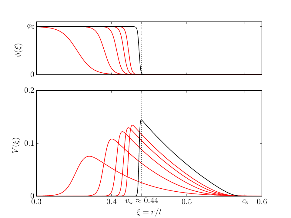
In the calculations leading to the above expressions it was assumed that the fluid kinetic energy was localised near the bubble wall, whereas in reality it reaches a scaling profile proportional to the bubble radius, meaning that the assumption of thin shells instantaneously colliding does not hold (see Fig. 1). Furthermore, the fluid kinetic energy persists as sound waves in the plasma after the transition, until turbulence and expansion attenuate this source.

In Ref. [29], it was argued that the actual energy deposited in gravitational waves by a fluid source is approximately

\tilde{\Omega}_{\text{GW}}^{\text{sound}}\simeq 3\left(\kappa\alpha_{T}\right)^{2}\left(H_{*}(8\pi)^{\frac{1}{3}}\frac{v_{\mathrm{w}}}{\beta}\right)\tilde{\Omega}^{\text{env}}_{\text{GW}}

(3)

– typically a factor $60(\beta/H_{*})$ larger than the envelope approximation result. The power spectrum of gravitational waves was also very different.

Therefore, the envelope approximation should not be used to fully describe phase transitions where a lot of kinetic energy ends up in the fluid. It may still remain valid for gravitational waves sourced by the collision of scalar field bubble walls, which do not scale. It may also model the initial collision of the fluid shells, if they are thin enough, such as in Jouguet detonations.

The various types of sources – scalar field collisions, fluid shell collisions, acoustic waves and turbulence – contribute to different extents, depending on the model.

The principal aim of this paper is to directly test the envelope approximation against a full lattice simulation for the first time, concentrating on the scalar field bubble walls in a thermal phase transition. This is motivated by two observations. First, collisions of the scalar field walls will always source gravitational waves (although the source may well be subdominant for a thermal phase transition). Second, in certain cases, such as where the wall runs away, scalar field collisions may be the dominant source of gravitational waves.

We will also investigate the suitability of the envelope approximation result for modelling the production of gravitational waves by colliding plasma shells. Immediately after the shells have collided, it does get the amplitude of gravitational waves approximately right, but the high-frequency and long-term behaviour of the gravitational wave power spectrum are both incorrect.

In Section II we review the production of gravitational waves by bubble collisions in the formalism of Ref. [30], and the approximations involved. Next, in Section III we give details of our numerical evaluation of the envelope approximation, and present the comparison of our results to those obtained previously.

The techniques used in direct numerical lattice simulations of the phase transition are reprised in Section IV, and comparisons with the envelope approximation are made. We discuss the results in Section V.

II Production of gravitational radiation

The quantity of interest is typically the fraction of energy emitted as gravitational waves per decade,

\Omega_{\text{GW}}=\omega\frac{\mathrm{d}E_{\text{GW}}}{\mathrm{d}\omega}\frac{1}{E_{\text{tot}}}\equiv\frac{\mathrm{d}E_{\text{GW}}}{\mathrm{d}\ln\omega}\frac{1}{E_{\text{tot}}}

(4)

where $E_{\text{tot}}$ is the total energy.

The gravitational wave power radiated in a direction $\hat{\mathbf{k}}$ at a frequency $\omega$ per unit solid angle $\Omega$ is [30]

\frac{\mathrm{d}E_{\text{GW}}}{\mathrm{d}\Omega\mathrm{d}\omega}=2G\omega^{2}\lambda_{ij,lm}(\hat{\mathbf{k}})\tau_{ij}^{*}(\hat{\mathbf{k}},\omega)\tau_{lm}(\hat{\mathbf{k}},\omega),

(5)

where $\Lambda_{ij,lm}$ is the projection tensor

\Lambda_{ij,lm}(\hat{\mathbf{k}})\equiv\delta_{il}\delta_{jm}-2\hat{\mathbf{k}}_{j}\hat{\mathbf{k}}_{m}\delta_{ij}+\frac{1}{2}\hat{\mathbf{k}}_{i}\hat{\mathbf{k}}_{j}\hat{\mathbf{k}}_{l}\hat{\mathbf{k}}_{m}\\ -\frac{1}{2}\delta_{ij}\delta_{lm}+\frac{1}{2}\delta_{ij}\hat{\mathbf{k}}_{l}\hat{\mathbf{k}}_{m}+\frac{1}{2}\delta_{lm}\hat{\mathbf{k}}_{i}\hat{\mathbf{k}}_{j};

(6)

and $\tau_{ij}(\hat{\mathbf{k}},\omega)$ is the Fourier transformed stress-energy tensor

\tau_{ij}(\hat{\mathbf{k}},\omega)=\frac{1}{2\pi}\int\mathrm{d}t\,e^{i\omega t}\int\mathrm{d}^{3}x\,e^{-i\omega\hat{\mathbf{k}}\cdot\mathbf{x}}\tau_{ij}(\mathbf{x},t).

(7)

For a scalar field $\phi$ , the source is given by

\tau^{\phi}_{ij}=\partial_{i}\phi\partial_{j}\phi

(8)

while for a relativistic fluid with energy $\epsilon$ , pressure $p$ , relativistic gamma factor $W$ and 3-velocity $V_{i}$ , the source is

\tau^{\mathrm{f}}_{ij}=W^{2}(\epsilon+p)V_{i}V_{j}

(9)

(the pieces proportional to the metric in the full stress-energy tensor are pure trace and hence do not source gravitational waves).

In addition to the linearised gravity approximation that yields the above expressions, two further simplifications are usually employed when computing the resulting gravitational wave power [19]. First, the collided portions of the bubbles are neglected; this is what is most strictly described as the envelope approximation. Second, the bubble walls are treated as sufficiently thin that the oscillatory part of the integral $e^{-i\omega\hat{\mathbf{k}}\cdot\mathbf{x}}$ is approximately constant in the region where $\tau_{ij}$ is nonzero.

The combination of the above approximations (often collectively referred to simply as the ‘envelope approximation’) has also been applied to thermal phase transitions, where the scalar field is coupled to a number of degrees of freedom that form a plasma [6]. One can compute an efficiency factor $\kappa^{\text{f}}$ for the conversion of vacuum energy into plasma kinetic energy [6, 20], and if one assumes that the shell of fluid is thin then the envelope approximation can be adapted to this case [9].

The resulting simple prediction of a broken power law form for the power spectrum from gravitational waves at a first-order phase transition has been widely adopted in the literature (see for example Refs. [31, 11, 12, 15]): an approximately $\omega^{3}$ dependence at low frequencies, and an approximately $\omega^{-1}$ dependence at high frequencies. The break occurs at a characteristic length scale, believed to be set by ratio of the inverse nucleation rate to the Hubble rate $(H_{*}/\beta)$ . Heuristically, the $\omega^{3}$ dependence can be seen as the absence of structure (‘white noise’) on longer length scales, while it has been argued that the approximate $\omega^{-1}$ dependence at short length scales can be attributed to the size distribution of bubbles. In the following section we will show that both power laws are intrinsic features of the set of approximations outlined above, irrespective of whether the bubbles are nucleated simultaneously or with a physically-motivated exponential rate.

The collision of a pair of scalar field bubbles was treated numerically in Ref. [18]. Since then, there have not been any further attempts to perform direct numerical simulations that compare the envelope approximation with dynamical vacuum scalar fields or field-fluid systems modelling thermal phase transitions. In Refs. [27, 29], a transient $\omega^{-1}$ power law was seen for the gravitational wave power spectrum at early times, which was attributed to the scalar field collisions. This assertion shall be tested in the present work.

III Computations in the envelope approximation

The envelope approximation consists of approximating the stress-energy of the bubble wall with an infinitesimally thin shell, yielding

$\displaystyle\tau_{ij}(\hat{\mathbf{k}},\omega)$	$\displaystyle=\kappa\rho_{\text{vac}}v_{\mathrm{b}}^{3}C_{ij}(\hat{\mathbf{k}},\omega)$	(10)
$\displaystyle C_{ij}(\hat{\mathbf{k}},\omega)$	$\displaystyle=\frac{1}{6\pi}\sum_{n}\int\mathrm{d}t\,e^{i\omega(t-\hat{\mathbf{k}}\cdot\mathbf{x}_{n})(t-t_{n}^{3})}A_{n,ij}(\mathbf{k},\omega)$	(11)
$\displaystyle A_{n,ij}(\hat{\mathbf{k}},\omega)$	$\displaystyle=\int_{S_{n}}\mathrm{d}\Omega\,e^{-i\omega v_{b}(t-t_{n})\hat{\mathbf{k}}\cdot\hat{\mathbf{x}}}\hat{\mathbf{x}}_{i}\hat{\mathbf{x}}_{j}.$	(12)

If the source under study is a system of intersecting fluid shells, then the efficiency factor $\kappa=\kappa^{\mathrm{f}}$ can be computed according the the procedure in Ref. [20]. For scalar field bubble walls, an effective scalar field efficiency factor $\kappa^{\phi}$ can be calculated from the energy density on the bubble walls and the surface area of the bubbles.

We evaluate Eqs. (10-12) using the method given in Ref. [9]. By choosing a system of cylindrical coordinates such that $\hat{\mathbf{k}}$ is aligned with the $z$ -axis, the projected stress-energy tensor becomes

\Lambda_{ij,lm}\tau^{*}_{ij}\tau_{lm}\\ =\frac{1}{2}(\tau^{*}_{xx}-\tau^{*}_{yy})(\tau_{xx}-\tau_{yy})+\tau_{xy}^{*}\tau_{xy}+\tau^{*}_{yx}\tau_{yx},

(13)

and the integrations over $C_{ij}$ and $A_{ij}$ become much simpler. We need simply compute

	$\displaystyle C_{\pm}(\omega)$	$\displaystyle=\frac{1}{6\pi}\,\sum_{n}^{N_{\mathrm{b}}}\int\mathrm{d}t\,e^{i\omega(t-z_{n})}(t-t_{n})^{3}A_{n,\pm}(\omega,t)$		(14)
	$\displaystyle A_{n,\pm}(\omega,t)$	$\displaystyle=\int_{-1}^{1}\mathrm{d}z\,e^{-iv_{\mathrm{b}}\omega(t-t_{n})z}B_{n,\pm}(z,t)$		(15)

where

	$\displaystyle B_{n,+}(z,t)$	$\displaystyle=\frac{(1-z^{2})}{2}\int_{S^{\prime}_{n}}\mathrm{d}\phi\,\cos(2\phi),$		(16)
	$\displaystyle B_{n,-}(z,t)$	$\displaystyle=\frac{(1-z^{2})}{2}\int_{S^{\prime}_{n}}\mathrm{d}\phi\,\sin(2\phi).$		(17)

See the appendix of Ref. [9] for more details. The summation over $n$ is a sum over all $N_{\mathrm{b}}$ bubbles in the simulation volume, and the integration region $S^{\prime}_{n}$ is the area on the surface of the $n$ th bubble that does not intersect with any other bubble.

To compute the envelope approximation for a fixed volume we not only simulate the bubbles within the volume, but also follow the development of bubbles in adjacent boxes (see Fig. 2). We impose periodic boundary conditions on our box, so we nucleate image bubbles in adjacent boxes. These do not contribute to the power but are included in the evaluation of the uncollided bubble regions. This is in contrast to Refs. [9, 19], where a spherical volume is used, but has the advantage that we can make truly direct comparisons with lattice simulations. This means we must consider the interactions of up to $27N_{\mathrm{b}}-1$ other bubbles when determining the contribution of the $n$ th bubble to the total power, although in practice the number of bubbles in range is much smaller.

Our approach to computing the envelope approximation is therefore about an order of magnitude more computationally intensive than previous studies although the number of bubbles participating is around the same. For comparisons with coupled field-fluid simulations, this is not an issue as the dynamic range available there is a more pressing constraint.

The fitted broken power law ansatz for the envelope approximation was given in Eq. (1) – a positive power law with index $a$ at low wavenumber and a negative power law with $b$ at high wavenumber. This also describes our own computations with the envelope approximation and so curves given by fits to Eq. 1 will be shown alongside our simulation results in the following sections.

The theoretical expectation is that the low-frequency rising power law has index $a=3$ , due to causality – there is nothing in the system on length scales larger than the largest bubble, so a cubic power law is anticipated (two powers of $\omega$ from the radial integral, and one additional power). We have confirmed this in our envelope approximation simulations.

For the high-frequency power law, it is widely expected that $b\approx 1$ , either due to the size distribution of bubbles or intrinsic effects. Unfortunately, we cannot reach high enough frequencies $\omega$ to verify that $b$ is exactly unity.

However, we will show that these exponents are intrinsic to the envelope approximation and do not depend on, for example, nucleation rate. Later, we will also show that colliding scalar field bubble walls give the same power laws.

III.1 Testing the envelope approximation: geometry and nucleation rate

It is standard to model the nucleation probability per unit volume and time $P$ by

P=P_{0}e^{\beta(t-t_{0})},

(18)

with $\beta$ computed, in principle, from the bounce action [32, 33, 34, 35]. We instead take $\beta$ to be a constant numerical value throughout our simulations in this section (in some cases we make it effectively infinite: we nucleate bubbles simultaneously).

In this section, we consider the results of simulations with $v_{\text{w}}=1$ , 109 bubbles and $\beta=1$ or $\beta\to\infty$ . For a given bubble distribution, our results are the average of 32 uniformly distributed random choices of the $z$ -axis in Eq. (13).

In Fig. 3, we choose a single spatial distribution of bubbles and nucleate them either over time with rate parametrised by the ‘realistic’ $\beta=1$ , or simultaneously. For this bubble distribution, a bootstrapped fit to Eq. (1) for $\omega\in[0.01,100]$ yields $a=3.05\pm 0.03$ , $b=0.62\pm 0.05$ for the ‘realistic’ case. For the simultaneous case, we obtain $a=2.98\pm 0.02$ and $b=0.65\pm 0.04$ . The power laws at high frequencies in the envelope approximation are therefore not dependent on the size distribution of bubbles at the end of the phase transition.

We have confirmed that these fitted power laws do not change substantially when averaged over eight different bubble distributions.

We can do even more with the simultaneously nucleated simulation. The resulting power spectrum can be rescaled to give the gravitational wave power spectrum for a physical nucleation rate. Given Eq. (5), we can write the rescaled gravitational wave power as

\omega\frac{\mathrm{d}E_{\text{GW}}}{\mathrm{d}\omega}=\omega\sum_{n}^{N_{\mathrm{b}}}\frac{v_{\mathrm{w}}^{3}(t_{\text{end}}-t_{0,n})^{3}}{\mathcal{V}}\\ \times 2G\tilde{\omega}_{n}^{2}\lambda_{ij,lm}(\hat{\mathbf{k}})\tau_{ij}^{*}\left(\hat{\mathbf{k}},\tilde{\omega}_{n}\right)\tau_{lm}\left(\hat{\mathbf{k}},\tilde{\omega}_{n}\right)

(19)

with

\tilde{\omega}_{n}=\frac{v_{\mathrm{w}}(t_{\text{end}}-t_{0,n})}{(\mathcal{V}/N_{\mathrm{b}})^{1/3}}\omega,

(20)

where $\mathcal{V}$ is the volume and the summation is over each bubble, the $n$ th bubble being nucleated at time $t_{0,n}$ , the phase transition ends at around $t_{\text{end}}$ . The numerator is therefore the approximate radius of the $n$ th bubble, while the denominator $(\mathcal{V}/N_{\mathrm{b}})^{1/3}$ is the average bubble radius in the simulation where all bubbles were nucleated simultaneously. For concreteness, we measure the remaining exposed surface area as a function of time and take $t_{\text{end}}$ as the time when the surface area of uncollided bubbles is less than 1% of its peak value.

The result of applying this rescaling is also shown in Fig. 3, with good agreement. A similar rescaling argument would presumably apply to the acoustic source in Ref. [29]. As the bubbles collide at different times, fixing $t_{\text{end}}$ is an oversimplification, but it works surprisingly well.

In summary, then, it is clear that the power laws seen in the envelope approximation are an intrinsic feature of the calculation, rather than the distribution of bubbles. It is also possible to reweight gravitational wave power spectra produced at equal times to more realistic distributions.

IV Direct simulations of the field-fluid system

Having performed some tests of our new envelope approximation code against the existing envelope approximation literature, we now wish to make a comparison against the power spectra provided by lattice simulations.

The equations and parameter choices we use have been discussed extensively elsewhere [36, 37, 38, 39, 40, 41, 27, 29], so we present only a brief summary here. We are working with a coupled system of a relativistic ideal fluid $U^{\mu}$ and scalar field $\phi$ , with energy-momentum tensor

T^{\mu\nu}=\partial^{\mu}\phi\partial^{\nu}\phi-{\textstyle\frac{1}{2}}g^{\mu\nu}(\partial\phi)^{2}+\left[\epsilon+p\right]U^{\mu}U^{\nu}+g^{\mu\nu}p,

(21)

where the metric is $g^{\mu\nu}=\mathrm{diag}(-1,1,1,1)$ . The system has an effective potential

V(\phi,T)=\frac{1}{2}\gamma(T^{2}-T_{0}^{2})\phi^{2}-\frac{1}{3}\alpha T\phi^{3}+\frac{1}{4}\lambda\phi^{4},

(22)

with parameters given in Table 1. The equation of state is

	$\displaystyle\epsilon(T,\phi)$	$\displaystyle=3aT^{4}+V(\phi,T)-T\frac{\partial V}{\partial T},$		(23)
	$\displaystyle p(T,\phi)$	$\displaystyle=aT^{4}-V(\phi,T),$		(24)

$a=(\pi^{2}/90)g_{*}$ ; we take $g_{*}=34.25$ for consistency with previous papers. From the energy-momentum tensor we can derive equations of motion. The system is decomposed into our choice of ‘field’ and ‘fluid’ parts,

$\displaystyle[\partial_{\mu}T^{\mu\nu}]_{\rm field}$	$\displaystyle=(\partial_{\mu}\partial^{\mu}\phi)\partial^{\nu}\phi-\frac{\partial V}{\partial\phi}\partial^{\nu}\phi$
	$\displaystyle\qquad=\eta U^{\mu}\partial_{\mu}\phi\partial^{\nu}\phi,$	(25)
$\displaystyle[\partial_{\mu}T^{\mu\nu}]_{\rm fluid}$	$\displaystyle=\partial_{\mu}[(\epsilon+p)U^{\mu}U^{\nu}]-\partial^{\nu}p+\frac{\partial V}{\partial\phi}\partial^{\nu}\phi$
	$\displaystyle\qquad=-\eta U^{\mu}\partial_{\mu}\phi\partial^{\nu}\phi.$	(26)

The parameter $\eta$ sets the scale of the friction and, hence, the wall velocity.

We simulate the coupled field-fluid system using parameters familiar from Refs. [27, 29], summarised in Table 1 (again, for consistency with previous work, we use units where $G=T_{\mathrm{c}}=1$ ). The ‘weak’ and ‘weak scaled’ parameters give a phase transition strength $\alpha_{T_{\mathrm{N}}}\approx 0.01$ , while the ‘intermediate’ parameters give $\alpha_{T_{\mathrm{N}}}\approx 0.1$ .

	Weak	Weak (scaled)	Intermediate
$T_{0}/T_{\mathrm{c}}$	$1/\sqrt{2}$	$1/\sqrt{2}$	$1/\sqrt{2}$
$\gamma$	$1/18$	$4/18$	$2/18$
$\alpha$	$\sqrt{10}/72$	$\sqrt{10}/9$	$\sqrt{10}/72$
$\lambda$	$10/648$	$160/648$	$5/648$

Table 1: Potential parameters used for this paper. These are the same as for Refs. [27, 29]. The ‘weak scaled’ parameters give the same phase transition strength as the ‘weak’ parameters, but the bubble wall width is halved (see Table 2).

It was hoped that ‘scaled’ forms of the ‘intermediate’ parameters could also be used, to improve the dynamic range of the simulations, but in tests using a spherically symmetric code it was found that the resulting fluid shock at $v_{\mathrm{w}}=0.44$ cannot be resolved well with our current simulation code and available resources.

From the potential (22), we can compute the surface tension $\sigma$

\sigma=\frac{2\sqrt{2}}{81}\frac{\alpha^{3}}{\lambda^{5/2}}T_{\mathrm{c}}^{3}

(27)

and the correlation length in the broken phase $\ell$

\ell^{2}=\frac{9\lambda}{2\alpha^{2}}\frac{1}{T_{\mathrm{c}}^{2}}.

(28)

The latent heat at the critical temperature is

\mathcal{L}=\frac{\alpha^{2}\gamma}{\lambda^{2}}T_{0}^{2}T_{\mathrm{c}}^{2}

(29)

and the ratio of latent heat to radiation $\alpha_{T}$ can then be written as

\alpha_{T}=\frac{\mathcal{L}}{3aT^{4}}.

(30)

These derived quantities, along with other relevant quantities for the simulations, are shown in Table 2.

IV.1 Gravitational waves from colliding scalar field bubbles

In Ref. [29] it was conjectured that the $\omega^{-1}$ power law seen above the peak in the gravitational wave power spectrum was the same as that produced by the envelope approximation. In this section we shall test that hypothesis.

To make the comparison as exact as possible we compare bubbles nucleated in exactly the same positions for both the field-fluid model and the envelope approximation, although we note that even for $N_{\mathrm{b}}=37$ in Ref. [29] there was no noticeable difference between power spectra when bubbles were nucleated in different positions. Again, since the envelope approximation calculation outlined above only gives the power radiated in the specified $\hat{\mathbf{z}}$ -direction, we repeat the envelope approximation simulation for 32 randomly selected directions uniformly distributed on the surface of the sphere. As we are directly comparing lattice simulations and envelope approximation calculations for the same configuration, random errors quoted in this section are those arising from this sampling.

In Fig. 4, we rescale the gravitational wave power spectra for the ‘weak’, ‘weak scaled’ and ‘intermediate’ phase transition parameters by the respective scalar field energy densities. This shows that the ‘weak’ and ‘weak scaled’ cases give broadly similar power spectra, lying systematically about $1\sigma$ below most points in the envelope approximation. Agreement with the ‘intermediate’ parameters is not as good, perhaps because the increased surface tension deforms the bubbles as they collide.

In Fig. 5, we instead scale the envelope approximation and compare with the actual gravitational wave power spectrum for the ‘weak scaled’ parameters. Also shown are the broken-phase correlation length $\ell$ and the simulation box size $L$ , to give an indication of the limitations imposed by dynamic range. For this case, in Fig. 6 we also plot the dimensionless scalar field and fluid kinetic energy quantities:

	$\displaystyle\overline{U}_{\mathrm{f}}$	$\displaystyle=\sqrt{\frac{1}{\mathcal{V}(\overline{\epsilon}+\overline{p})}\int d^{3}x\,\tau_{ii}^{\mathrm{f}}},$		(31)
	$\displaystyle\overline{U}_{\phi}$	$\displaystyle=\sqrt{\frac{1}{\mathcal{V}(\overline{\epsilon}+\overline{p})}\int d^{3}x\,\tau_{ii}^{\phi}}.$		(32)

These are compared to the equivalent quantity $\overline{U}_{\phi,\text{env}}$ computed during a run of the envelope approximation based on the uncollided surface area and the scalar field gradient energy. There is very good agreement between $\overline{U}_{\phi}$ and $\overline{U}_{\phi,\text{env}}$ : the acceleration of the bubbles in the full simulation is seemingly of little importance to the scalar field source.

For the phase transition strengths studied here there is no evidence that the presence of fluid in front of the wall affects the power spectrum. The gravitational wave power spectrum sourced by the scalar field, shown in Figs. 4 and 5, does not change when the fluid part of the simulation is not evolved dynamically but the friction term is retained so that the wall velocity is unchanged.

IV.2 Gravitational waves from colliding fluid shells

We now turn our attention to the form of the fluid power spectrum immediately after the bubbles have collided, and hypothesise that the gravitational wave power produced by the fluid up to this point might still be computed with the envelope approximation. The later contribution due to sound waves must then be computed separately.

The computation proceeds as before, except that in Eq. (10) the energy density is scaled by the fraction $\kappa^{\mathrm{f}}$ of vacuum energy that gets turned into fluid kinetic energy as the bubbles grow. While in the scalar field case in the previous section, the energy density $\rho$ was estimated based on the surface of each bubble at collision, here we can directly measure the total fluid kinetic energy at the end of the transition and use it to compute an efficiency (see Table 2); this can also be computed analytically [20].

	Weak	Weak (scaled)	Intermediate
$\sigma/T_{\mathrm{c}}^{3}$	$1/10$	$1/20$	$4\sqrt{2}/10$
$\ell\,T_{\mathrm{c}}$	$6$	$3$	$6\sqrt{2}$
$\mathcal{L}/T_{\mathrm{c}}^{4}$	$9/40$	$9/40$	$9/5$
$\alpha_{T_{\mathrm{N}}}$	$0.010$	$0.010$	$0.084$
$\mathcal{V}\,T_{\mathrm{c}}^{3}$	$4800^{3}$	$4800^{3}$	$4800^{3}$
$N_{\mathrm{b}}$	$125$	$125$	$125$
$R_{*}$	$960$	$960$	$960$
$\mathcal{S}\,T_{\mathrm{c}}^{2}$	$6.98\times 10^{8}$	$6.98\times 10^{8}$	$6.98\times 10^{8}$
$\eta/T_{\mathrm{c}}$	$0.2$	$0.4$	$0.4$
$v_{\mathrm{w}}$	$0.44$	$0.44$	$0.44$
$\Sigma$	$0.136$	$0.068$	$0.776$
$\kappa^{\phi}\rho^{\text{vac}}/T_{\mathrm{c}}$	$0.000859$	$0.000430$	$0.00490$
$\kappa^{\mathrm{f}}$	$0.0348$	$0.0348$	$0.195$
$\kappa^{\mathrm{f}}\rho^{\text{vac}}/T_{\mathrm{c}}$	$0.000348$	$0.000348$	$0.0164$

Table 2: Table of various derived quantities and simulation parameters. The surface tension

\sigma

, broken phase correlation length

\ell

(approximately the bubble wall thickness) and phase transition strength

\alpha_{T_{\mathrm{N}}}

are computed from the parameters in Table 1 by means of Eqs. (27-30). The simulation volume

\mathcal{V}

and number of bubbles

N_{\mathrm{b}}

are set for each simulation, yielding the typical bubble radius

R_{*}=(\mathcal{V}/N_{b})^{1/3}

. The total collided ‘surface area’

\mathcal{S}

can be computed given the Voronoi partition of the nucleated bubble locations. The friction parameter

\eta

determines the wall velocity

v_{\mathrm{w}}

, chosen in each case to give a fast deflagration (such that

v_{\mathrm{w}}\approx 0.44

would be achieved if the bubbles could expand unimpeded). The scalar field gradient energy per unit area

\Sigma

is approximately proportional to

\sigma

. The scalar field energy density is then

\kappa^{\phi}\rho^{\text{vac}}=\Sigma\mathcal{S}/\mathcal{V}

, since the energy in the scalar field source scales only with the radius of the bubbles, whereas the fluid source scales with the volume and hence

\kappa^{\mathrm{f}}\rho^{\text{vac}}

can be computed analytically for the general case [20].

In Fig. 6 the dimensionless measure of the fluid kinetic energy density $\overline{U}_{\mathrm{f}}$ is shown, and as expected it remains approximately constant after the phase transition completes. Consequently, the acoustic waves present in the fluid continue to source gravitational waves, and in Fig. 7 the amplitude of the gravitational waves from the lattice simulation – shown in red – continues to grow after the phase transition has completed. The envelope approximation result, appropriately scaled by $\kappa^{f}\rho^{\text{vac}}$ , is also shown.

By comparing the fluid kinetic energy at the indicated time intervals of $500/T_{\mathrm{c}}$ in Fig. 6 with the succession of red curves in Fig. 7 – the fourth point and curve in particular – one can see that the envelope approximation gets the amplitude of the gravitational wave power produced by colliding fluid shells correct to within an order of magnitude at the time the fluid kinetic energy has reached its final value. The form of the power spectrum is, however, different; the peak is offset; and the total power continues to grow after this time, sourced by acoustic waves set up in the plasma after collision.

To be specific, up to the time at which the bubbles collide, there are two peaks – one closer to the infrared at $k_{\text{env}}\sim 1/R_{*}$ , and another at higher $k$ around the fluid shell thickness $k_{\text{shell}}\sim v_{\mathrm{w}}/(R_{*}|v_{\mathrm{w}}-c_{s}|)$ . In this case, $k_{\text{shell }}\approx 3k_{\text{env}}$ . The $k_{\text{shell}}$ peak continues to grow, sourced by acoustic waves in the fluid. Note also that the high- $k$ power law associated with this peak is steeper (approximately $k^{-3}$ ) than the envelope approximation. This peak continues to grow until extinguished by expansion on a timescale $1/H_{*}$ [29].

As a final note, in the $v_{\mathrm{w}}\approx 0.44$ , ‘weak parameter’ simulations discussed extensively here, the amplitude of gravitational waves sourced by the scalar field (shown in Fig. 5) and by the fluid (show in Fig. 7) are comparable, at least as the phase transition is ending. However, in a realistic scenario, the scalar field bubble walls would be much thinner than the fluid shell, and in any case, acoustic waves (and possibly turbulence) play a more important role, at least for thermal phase transitions.

V Discussion

We have revisited previous work employing the envelope approximation to compute the gravitational wave power spectrum from colliding bubbles. The observed power laws – which are consistent with what was seen in Ref. [9] – do not depend on the nucleation rate, and it is possible to reweight from simulations with simultaneous nucleation to more physical scenarios. We have no evidence that the hierarchy of bubble sizes affects the power law above the peak – the power laws are an intrinsic feature of the envelope approximation.

In addition, we compared the envelope approximation to large-scale lattice simulations of a thermal phase transition, where a scalar field expands in a plasma of light particles. The envelope approximation is a good model for the gravitational waves produced by the scalar field, although it seems to perform less well at higher surface tensions.

For gravitational waves sourced by the plasma, the envelope approximation gets the peak amplitude approximately correct, but the form of the power spectrum is incorrect. Furthermore, the subsequent acoustic and turbulent behaviour cannot be modelled at all.

This paper focused on fairly fast ( $v_{\mathrm{w}}=0.44$ ) subsonic deflagrations. In such cases the fluid shells are very thick, about a third the radius of the bubble itself. Future work will consider the possibility that the initial transient collision of very thin fluid shells – such as in the fine-tuned Jouguet case where $v_{\mathrm{w}}\approx c_{\mathrm{s}}$ – might be better described by the envelope approximation. At late times, though, the dominant sources will still be sound waves and turbulence.

It is expected that, for a viable first order electroweak-scale phase transition, the sources for which the envelope approximation would be valid – the scalar field bubble collisions, and possibly the initial fluid shell collisions – are subdominant. However, this is not necessarily the case, depending on $\beta/H_{*}$ , or if the bubble wall runs away. Our results are valuable in any case because they represent the first comparison of the envelope approximation with alternative methods of modelling gravitational waves. They also represent an external test of the ‘gravity sector’ of the simulation code in Refs. [27, 29].

We used novel boundary conditions for our envelope approximation calculation. When the ‘spherical cutoff’ approach is used, the number of pairs of bubble interactions that must be checked grows only as $N_{\mathrm{b}}^{2}$ , whereas in our hypercubic case, it grows as $27N_{\mathrm{b}}^{2}$ . Therefore, if we had adopted the standard technique, about five times as many bubbles could be simulated for the same amount of computing time.

There are important consequences for modelling the gravitational wave production from first-order phase transitions: the true peak may be shifted to higher $k$ by up to an order of magnitude, although the amplitude will be higher; and the power laws associated with the peak may well be steeper. These effects mean care must be taken when discussing the prospects for detection at future detectors such as eLISA [5].

We conclude by reaffirming the utility of the envelope approximation for modelling the immediate aftermath of a thermal phase transition, or for situations where the fluid does not contribute (such as vacuum bubbles). For the majority of cases – where the fluid source is dominant – an analytic or at least semi-analytic method is still lacking, and direct numerical simulation is still necessary.

Acknowledgements.

Our simulations made use of ‘gorina1’ at the University of Stavanger as well as the Abel cluster, a Notur facility. We acknowledge PRACE for awarding us access to resource HAZEL HEN based in Germany at the High Performance Computing Center Stuttgart (HLRS). We acknowledge useful discussions with Mark Hindmarsh, Stephan Huber, Kari Rummukainen and Anders Tranberg. Our work was supported by the People Programme (Marie Skłodowska-Curie actions) of the European Union Seventh Framework Programme (FP7/2007-2013) under grant agreement number PIEF-GA-2013-629425.

References

[1] T. Accadia et al., in Proceedings, 12th Marcel Grossmann Meeting on General Relativity, Paris, France, July 12-18, 2009. Vol. 1-3 (2009), pp. 1738–1742.
[2] G. M. Harry (LIGO Scientific), Class.Quant.Grav. 27, 084006 (2010).
[3] B. P. Abbott et al. (Virgo, LIGO Scientific), Phys. Rev. Lett. 116, 061102 (2016), eprint 1602.03837.
[4] P. A. Seoane et al. (eLISA) (2013), eprint 1305.5720.
[5] C. Caprini et al., JCAP 1604, 001 (2016), eprint 1512.06239.
[6] M. Kamionkowski, A. Kosowsky, and M. S. Turner, Phys.Rev. D49, 2837 (1994), eprint astro-ph/9310044.
[7] R. Apreda, M. Maggiore, A. Nicolis, and A. Riotto, Nucl. Phys. B631, 342 (2002), eprint gr-qc/0107033.
[8] C. Grojean and G. Servant, Phys. Rev. D75, 043507 (2007), eprint hep-ph/0607107.
[9] S. J. Huber and T. Konstandin, JCAP 0809, 022 (2008), eprint 0806.1828.
[10] A. Ashoorioon and T. Konstandin, JHEP 07, 086 (2009), eprint 0904.0353.
[11] J. Kozaczuk, S. Profumo, L. S. Haskins, and C. L. Wainwright, JHEP 01, 144 (2015), eprint 1407.4134.
[12] G. C. Dorsch, S. J. Huber, and J. M. No, Phys. Rev. Lett. 113, 121801 (2014), eprint 1403.5583.
[13] M. Kakizaki, S. Kanemura, and T. Matsui, Phys. Rev. D92, 115007 (2015), eprint 1509.08394.
[14] L. Leitao and A. Megevand, JCAP 1605, 037 (2016), eprint 1512.08962.
[15] P. Schwaller, Phys. Rev. Lett. 115, 181101 (2015), eprint 1504.07263.
[16] J. Jaeckel, V. V. Khoze, and M. Spannowsky (2016), eprint 1602.03901.
[17] P. S. B. Dev and A. Mazumdar, Phys. Rev. D93, 104001 (2016), eprint 1602.04203.
[18] A. Kosowsky, M. S. Turner, and R. Watkins, Phys.Rev. D45, 4514 (1992).
[19] A. Kosowsky and M. S. Turner, Phys.Rev. D47, 4372 (1993), eprint astro-ph/9211004.
[20] J. R. Espinosa, T. Konstandin, J. M. No, and G. Servant, JCAP 1006, 028 (2010), eprint 1004.4187.
[21] C. Caprini, R. Durrer, and G. Servant, Phys. Rev. D77, 124015 (2008), eprint 0711.2593.
[22] C. Caprini, R. Durrer, T. Konstandin, and G. Servant, Phys.Rev. D79, 083519 (2009a), eprint 0901.1661.
[23] R. Jinno and M. Takimoto (2016), eprint 1605.01403.
[24] A. Kosowsky, A. Mack, and T. Kahniashvili, Phys. Rev. D66, 024030 (2002), eprint astro-ph/0111483.
[25] T. Kahniashvili, A. Kosowsky, G. Gogoberidze, and Y. Maravin, Phys. Rev. D78, 043003 (2008), eprint 0806.0293.
[26] C. Caprini, R. Durrer, and G. Servant, JCAP 0912, 024 (2009b), eprint 0909.0622.
[27] M. Hindmarsh, S. J. Huber, K. Rummukainen, and D. J. Weir, Phys.Rev.Lett. 112, 041301 (2014), eprint 1304.2433.
[28] J. T. Giblin and J. B. Mertens, Phys.Rev. D90, 023532 (2014), eprint 1405.4005.
[29] M. Hindmarsh, S. J. Huber, K. Rummukainen, and D. J. Weir, Phys. Rev. D92, 123009 (2015), eprint 1504.03291.
[30] S. Weinberg, Gravitation and Cosmology (Wiley, New York, 1972).
[31] C. Caprini, R. Durrer, and X. Siemens, Phys.Rev. D82, 063511 (2010), eprint 1007.1218.
[32] S. R. Coleman, Phys. Rev. D15, 2929 (1977), [Erratum: Phys. Rev.D16,1248(1977)].
[33] C. G. Callan, Jr. and S. R. Coleman, Phys. Rev. D16, 1762 (1977).
[34] A. D. Linde, Nucl. Phys. B216, 421 (1983), [Erratum: Nucl. Phys.B223,544(1983)].
[35] K. Enqvist, J. Ignatius, K. Kajantie, and K. Rummukainen, Phys. Rev. D45, 3415 (1992).
[36] K. Kajantie and H. Kurki-Suonio, Phys.Rev. D34, 1719 (1986).
[37] J. Ignatius, K. Kajantie, H. Kurki-Suonio, and M. Laine, Phys.Rev. D49, 3854 (1994a), eprint astro-ph/9309059.
[38] J. Ignatius, K. Kajantie, H. Kurki-Suonio, and M. Laine, Phys.Rev. D50, 3738 (1994b), eprint hep-ph/9405336.
[39] H. Kurki-Suonio and M. Laine, Phys.Rev. D51, 5431 (1995), eprint hep-ph/9501216.
[40] H. Kurki-Suonio and M. Laine, Phys.Rev. D54, 7163 (1996a), eprint hep-ph/9512202.
[41] H. Kurki-Suonio and M. Laine, Phys.Rev.Lett. 77, 3951 (1996b), eprint hep-ph/9607382.