Balanced Ranking Mechanisms Thanks: We are grateful to Dilip Abreu, Attila Ambrus, Claude d’Aspremont, Sushil Bikhchandani, Rahul Deb, Bhaskar Dutta, Ed Green, Matt Jackson, Eric Maskin, Motty Perrry, Arunava Sen, Ricard Torres, Levent Ulku, Dan Vincent and seminar participants at ITAM, ISI Delhi, and Delhi School of Economics for useful comments.

Debasis Mishra Tridib Sharma ^†^†thanks: Debasis Mishra: Indian Statistical Institute, Delhi, dmishra@isid.ac.in; dmishra@gmail.com; Tridib Sharma: ITAM, Mexico, sharma@itam.mx

August 24, 2026

Abstract

In the private values single object auction model, we construct a satisfactory mechanism - a symmetric, dominant strategy incentive compatible, and budget-balanced mechanism. Our mechanism allocates the object to the highest valued agent with more than 99% probability provided there are at least 14 agents. It is also ex-post individually rational. We show that our mechanism is optimal in a restricted class of satisfactory ranking mechanisms. Since achieving efficiency through a dominant strategy incentive compatible and budget-balanced mechanism is impossible in this model, our results illustrate the limits of this impossibility.

Keywords. budget-balanced mechanisms, Green-Laffont mechanism, Pareto optimal mechanism.

JEL Keywords. D82, D71, D02.

1 Introduction

How should a group of agents allocate a unit of resource among themselves? For instance, consider the problem of allocating a bequest among a group of potential heirs. Many a times, no will exists. Even when a will exists, disputes arise. Designated estate agents are often employed to resolve bequest related problems. A Wall Street Journal article quotes an expert suggesting the following dispute resolution procedure:

In family disputes, Ms. Olsavsky says, one option is to have all the items put up for auction. Family members can bid on what they want. The money goes back to the estate to be divided equally (Coombs, 2013).

There are a number of other examples: a group of firms sharing time slots on a jointly owned supercomputer (Guo et al., 2011); a group of municipalities deciding on the location of a stadium (Cramton et al., 1987). A key feature of these problems is that transfers can be used (either as taxes or subsidies) for resource allocation. However, transfers across agents have to balance - money raised by auctioning a bequest must be redistributed among the heirs. ¹¹ 1 Commenting on the recent controversy surrounding the allocation of soccer World cup venue, Rakesh Vohra in the popular blog The Leisure of the Theory Class writes: Instead of running beauty contests to decide where to hold FIFA events, auction off the right to the highest bidder. This can be done in two ways. Allow each FIFA official with a vote to auction off their vote to the highest bidder. Or, do away with the officials altogether and have countries bid directly for the right to hold FIFA events. Full transparency, no bribery and FIFA may be richer than before! (Vohra, 2015) Just like the bequest settlement case, FIFA must redistribute the transfers collected from the countries among them.

We design mechanisms for such problems with the aim of achieving efficiency. Efficiency requires one to allocate the bequest to the highest valued heir or to allocate the world cup venue to the country which benifits the most from hosting the event. In the standard private values model, where each agent has a value for the unit of resource/object and transfers are allowed with quasilinear utility, the Vickrey auction satisfies three compelling desiderata of a mechanism: (a) dominant strategy incentive compatibility (DSIC), (b) (allocative) efficiency - allocating the object to the highest valuation agent, and (c) ex-post individual rationality. A well-known criticism of the Vickrey auction is that it is not budget-balanced - it collects revenue from the agents, which distorts ex-post efficiency. Green and Laffont (1979) shows that this criticism applies to every DSIC and efficient mechanism: no DSIC and efficient mechanism can be budget-balanced. We look for a second-best solution, where we explore the limits of this impossibility result:

How close to efficiency can we get using a DSIC and budget-balanced mechanism?

We require our solution to satisfy symmetry - agents with identical valuation must get the object with equal probability and pay the same amount. Symmetry is a compelling fairness property - for instance, in the bequest allocation problem, an asymmetric mechanism may either be unacceptable to potential heirs or lead to unpleasant lawsuits later on.

We identify a class of DSIC, budget-balanced, and symmetric mechanisms that we call ranking mechanisms. A ranking mechanism is one that uses a ranking allocation rule, which is specified (for $n$ agents) by $n$ numbers $(\pi_{1},\ldots,\pi_{n})$ between $0$ and $1$ such that they add up to not more than $1$ and $\pi_{j}\geq\pi_{j+1}$ for each $j$ . For every $j$ , the number $\pi_{j}$ is the probability with which an agent with the $j$ -th highest value is allocated the object at any generic profile of values. Our main result is a description of the r-optimal mechanism - a DSIC, budget-balanced, and symmetric ranking mechanism that beats every such mechanism in terms of the allocation probability to the highest valuation agent.

At every profile of values, our r-optimal mechanism allocates the object to the highest valued agent with more than 99% probability, provided there are at least 14 agents. It is also ex-post individually rational. The welfare generated by the r-optimal mechanism converges to efficiency as the number of agents increase. The nature of convergence is shown in Table 1, where we report on the probability with which the highest valued agent gets the object in our mechanism.

No of agents	Probability to the highest valued agent
$9$	$92.3\%$
$10$	$95\%$
$11$	$96.2\%$
$12$	$98.1\%$
$13$	$98.9\%$
$14$	$99.4\%$
$15$	$99.6\%$
$16$	$99.8\%$
$17$	$99.9\%$

Table 1: Convergence in our mechanism

The r-optimal mechanism we identify satisfies ex-post individual rationality. Ex-post individual rationality is a desired property of mechanisms. Consider politicians across municipalities or countries, involved in procuring a public facility or negotiating the venue of an international sporting event. Failure to get the facility or the event would result in criticisms. The criticism would be compounded if in addition to a failure, payments also have to be made. Political opponents could well allege corruption.

Ranking mechanisms contain two familiar DSIC, budget-balanced, and symmetric mechanisms: (i) the mechanism that allocates the object to each agent with equal probability without using any transfers and (ii) the residual claimant mechanism in Green and Laffont (1979). The residual claimant mechanism is defined by choosing an agent uniformly at random as a residual claimant and conducting a Vickrey auction among the other agents. The revenue generated from the auction is then given to the residual claimant. We refer to this mechanism as the Green-Laffont (GL) mechanism, and note that at profiles of distinct values, it allocates the object to the highest valued agent with probability $1-1/n$ and to the second highest valued agent with probability $1/n$ . ²² 2 This mechanism (and its variants) were discussed in the context of public-good provision problem in Green and Laffont (1979). Later, Gary-Bobo and Jaaidane (2000) formally define this mechanism and study its statistical and strategic properties. Our r-optimal mechanism coincides with the GL mechanism if the number of agents is no more than $8$ but differs from it significantly for more than $8$ agents.

Our analysis is prior-free. We use DSIC as our solution concept. As we discuss later in Section 5, Cramton et al. (1987) show that Bayesian incentive compatible, efficient, and budget-balanced mechanisms satisfying a form of individual rationality exists in our model. While the mechanism they propose require information about beliefs of agents (with common prior assumption), our result shows the level of efficiency that can be achieved using DSIC and budget-balanced mechanisms, thus showing the limits of such a prior-free and robust approach in this problem. Inspired by the seminal work of Bergemann and Morris (2005), recent literature in mechanism design has been investigating such questions in other models (Chung and Ely, 2007; Carroll, 2015). ³³ 3 There are two recent papers which also provide foundational results of DSIC mechanisms in the private values single object auction environment. Manelli and Vincent (2010) show that in such models, for every Bayesian incentive compatible mechanism, there is an “equivalent” DSIC mechanism - this equivalence is in terms of interim expected utility of agents. This result is extended to other settings in Gershkov et al. (2013). Unlike our work, these papers do not impose budget-balance as a constraint - indeed, these equivalence results do not hold if budget-balance constraint is imposed.

In view of the Green and Laffont impossibility result, comparing efficiency levels of two DSIC, budget-balanced, and symmetric mechanisms is a natural question. The notion we use here compares ranking mechanisms by the probability with which the highest valued agent gets the object. Formally, we show that this notion coincides with a worst-case measure of efficiency: the worst-case ratio of welfare generated by a ranking mechanism and efficient level of welfare. In a prior-free environment, such worst-case measures give a very robust method of comparing mechanisms. These measures are widely used to compare algorithms in the computer science literature, and in the algorithmic game theory literature (Cavallo, 2006; Guo and Conitzer, 2009). They are also becoming popular in the mechanism design literature (Chung and Ely, 2007; Moulin, 2009; Carroll, 2015; Massó et al., 2015).

From a technical point, our paper extends the Myersonian approach. Recall that Myerson (1981) provides necessary and sufficient conditions for a mechanism to be DSIC. ⁴⁴ 4 His characterization is for Bayesian incentive compatible mechanisms, but can be straightforwardly adapted to DSIC mechanisms. We extend his characterization to give necessary and sufficient conditions for a mechanism to be DSIC, budget-balanced, and symmetric. One of the surprising corollaries of this characterization is that if there is a DSIC, budget-balanced, and symmetric mechanism using an allocation rule, then it is the only such mechanism using this allocation rule. A consequence of this result is that the search over the domain of DSIC, budget-balanced, and symmetric mechanisms can be confined to the domain of allocation rules satisfying our necessary and sufficient conditions - we do not have to worry about payments since they are identified uniquely. Our characterization reveals a rich but complex class of such mechanisms. The ranking mechanisms that we consider in this paper are much simpler to describe. The separation of payment and allocation decisions gives us a lot of tractability in the class of ranking allocation rules, where we derive our mechanism and show its constrained optimality. Though we do not know if we can improve upon our r-optimal mechanism, by considering more complex mechanisms, the overwhelming speed of convergence of our mechanism (as shown in Table 1) implies that we may not be losing out much by restricting attention to ranking mechanisms.

The rest of the paper is organized as follows. We present our model in Section 2. We introduce ranking mechanisms and discuss our main results in Section 3. We give a technical characterization of DSIC, budget-balanced, and symmetric mechanisms in Section 4. We relate our results to the literature in Section 5 and conclude in Section 6. All the omitted proofs are relegated to an Appendix at the end. To keep the proofs of our results lucid, we present them in a different sequence than the sequence in which corresponding results appear in the main text. Hence, we recommend that the proofs be read after reading the main text.

2 The Model

We consider the standard single object independent private values model with $N=\{1,\ldots,n\}$ as the set of agents. Throughout, we assume that $n\geq 3$ - the $n=1$ case is trivial and the $n=2$ case is discussed later. Each agent $i\in N$ has a valuation $v_{i}$ for the object. If he is given $\alpha_{i}\in[0,1]$ of the object, or given the object with probability $\alpha_{i}$ , and he pays $p_{i}$ for it, then his net utility is $\alpha_{i}v_{i}-p_{i}$ . The set of all valuations for any agent is given by $V\equiv[0,\beta]$ , where $\beta\in\mathbb{R}$ . A valuation profile will be denoted by $\mathbf{v}\equiv(v_{1},\ldots,v_{n})$ .

An allocation rule is a map $f:V^{n}\rightarrow[0,1]^{n}$ , where we denote by $f_{i}(\mathbf{v})$ the probability of agent $i$ getting allocated the object at valuation profile $\mathbf{v}$ . We assume that at all $\mathbf{v}\in V^{n}$ , $\sum_{i\in N}f_{i}(\mathbf{v})\leq 1$ .

A payment rule of agent $i$ is a map $p_{i}:V^{n}\rightarrow\mathbb{R}$ . A collection of payment rules of all the agents will be denoted by $\mathbf{p}\equiv(p_{1},\ldots,p_{n})$ . A mechanism is a pair $(f,\mathbf{p})$ . We require our mechanism to satisfy the following three properties:

•

A mechanism $(f,\mathbf{p})$ is dominant strategy incentive compatible (DSIC) if for every $i\in N$ , for every $v_{-i}\in V^{n}$ , and for every $v_{i},v^{\prime}_{i}\in V$ , we have

v_{i}f_{i}(v_{i},v_{-i})-p_{i}(v_{i},v_{-i})\geq v_{i}f_{i}(v^{\prime}_{i},v_{-i})-p_{i}(v^{\prime}_{i},v_{-i}).

•

A mechanism $(f,\mathbf{p})$ is budget-balanced (BB) if for every $\mathbf{v}\in V^{n}$ , we have

$\sum_{i\in N}p_{i}(\mathbf{v})=0.$
•

A mechanism $(f,\mathbf{p})$ is symmetric if for every $\mathbf{v}\in V^{n}$ and for every $i,j\in N$ with $v_{i}=v_{j}$ , we have

$f_{i}(\mathbf{v})=f_{j}(\mathbf{v}),~~~~p_{i}(\mathbf{v})=p_{j}(\mathbf{v}).$

We call a mechanism satisfactory if it is DSIC, BB, and symmetric. ⁵⁵ 5 Green and Laffont (1977) use the terminology satisfactory mechanism to mean something different. Among other things, their satisfactory mechanisms are DSIC and efficient but need not be BB and symmetric. We apologize if this creates a confusion. Symmetry allows us to consider a mild notion of fairness in our mechanism. It also explicitly rules out dictatorial mechanisms, where a dictator agent is given the object for free at all valuation profiles. ⁶⁶ 6 A weaker version of symmetry would be to consider anonymity of the mechanism with respect to net utilities of the agents - see Sprumont (2013) for a formal definition. We will require our stronger version of symmetry for our main result.

An allocation rule $f$ is satisfactorily implementable if there exists a $\mathbf{p}$ such that $(f,\mathbf{p})$ is a satisfactory mechanism. We are interested in finding satisfactory mechanisms that are almost efficient in the following sense.

At any valuation profile $\mathbf{v}$ , denote by $\mathbf{v}[k]$ the set of agents who have the $k$ -th highest valuation at $\mathbf{v}$ . More formally,

\mathbf{v}[1]:=\{i\in N:v_{i}\geq v_{j}~\forall~j\in N\}.

Having defined $\mathbf{v}[k-1]$ , we recursively define $\mathbf{v}[k]$ as

\mathbf{v}[k]:=\{i\in N\setminus(\cup_{k^{\prime}=1}^{k-1}\mathbf{v}[k^{\prime}]):v_{i}\geq v_{j}~\forall~j\in N\setminus(\cup_{k^{\prime}=1}^{k-1}\mathbf{v}[k^{\prime}])\}.

Definition 1

An allocation rule $f$ is efficient at $\mathbf{v}$ if

\sum_{i\in\mathbf{v}[1]}f_{i}(\mathbf{v})=1.

An allocation rule $f$ is efficient if it is efficient at all $\mathbf{v}\in V^{n}$ . A mechanism $(f,\mathbf{p})$ is efficient if $f$ is efficient.

The efficiency of a BB mechanism is equivalent to maximizing the total welfare of agents at every profile of valuations. To see this, note that the total welfare of agents at a valuation profile $\mathbf{v}$ from a mechanism $(f,\mathbf{p})$ is

\sum_{i\in N}\Big[v_{i}f_{i}(\mathbf{v})-p_{i}(\mathbf{v})\Big]=\sum_{i\in N}v_{i}f_{i}(\mathbf{v}),

where the second equality followed from BB. This is clearly maximized by assigning the object to the highest valued agents.

Green and Laffont (1979) show that no DSIC and budget-balanced mechanism can be efficient. Hence, a satisfactory mechanism cannot be efficient. The precise question we are interested in is: what is the “most" efficient satisfactory mechanism?

2.1 A Prior-Free Notion to Measure Efficiency

In view of the Green-Laffont result, we adopt one of the well-known notions to measure efficiency of satisfactory mechanisms. Fix a satisfactory mechanism $\mathcal{M}\equiv(f,\mathbf{p})$ . Note that at any valuation profile $\mathbf{v}$ with $v_{1}\geq\ldots\geq v_{n}$ , the maximum possible (efficient) social welfare is $v_{1}$ , and the social welfare achieved by $\mathcal{M}$ is

\sum_{i\in N}v_{i}f_{i}(\mathbf{v}).

The ratio of these two numbers is a good measure of efficiency at the valuation profile $\mathbf{v}$ . More precisely, the number

f_{1}(\mathbf{v})+\frac{1}{v_{1}}\Big(\sum_{i\neq 1}v_{i}f_{i}(\mathbf{v}))\Big),

is a measure of efficiency at the valuation profile $\mathbf{v}$ . Here, as in the rest of the paper, we assume $\frac{0}{0}=1$ . Note that such a measure only depends on $f$ and not on $\mathbf{p}$ because $(f,\mathbf{p})$ is a budget-balanced mechanism. Now, the worst-case of this ratio happens when we minimize this over all $\mathbf{v}$ . In particular, for a satisfactory mechanism $\mathcal{M}\equiv(f,\mathbf{p})$ , the worst-case efficiency is given by

\mu^{\mathcal{M}}=\inf_{\mathbf{v}}\Bigg[f_{1}(\mathbf{v})+\frac{1}{v_{1}}\Big(\sum_{i\neq 1}v_{i}f_{i}(\mathbf{v}))\Big)\Bigg].

A natural objective is to find a satisfactory mechanism that maximizes this worst-case efficiency. As discussed in the introduction, this is a robust method of comparing efficiency of mechanisms. We apply this notion of comparing efficiency levels of mechanisms in a restricted class of mechanisms that we describe next.

3 Ranking Mechanisms

In most of the paper, we focus attention on the following class of simple allocation rules and the corresponding satisfactory mechanisms that can be constructed using such allocation rules. We call them ranking allocation rules. Each ranking allocation rule is defined by $n$ numbers $(\pi_{1},\ldots,\pi_{n})$ with each $\pi_{i}\in[0,1]$ and $\sum_{i\in N}\pi_{i}\leq 1$ . Informally, at a generic valuation profile $v_{1}>v_{2}>\ldots>v_{n}$ , for every $k$ , $\pi_{k}$ reflects the probability with which agent $k$ (which has rank $k$ at this profile) gets the object. Notice that this probability does not change across valuation profiles as long as the rank of the agent does not change. This feature makes the ranking allocation rules simple, both from the point of view of practical implementation and analysis. Also, we require every ranking allocation rule to be symmetric, and this means that it allocates the object in a particular way when there are ties in valuations. We clarify this tie-breaking by formally defining the ranking allocation rule first.

Definition 2

An allocation rule $f$ is a ranking allocation rule if it is symmetric and there exists numbers $\pi_{i}\in[0,1]$ for all $i\in N$ with $\pi_{1}\geq\ldots\geq\pi_{n}$ and $\sum_{i\in N}\pi_{i}\leq 1$ such that at every valuation profile $\mathbf{v}$ and every $k\in N$ , we have

\sum_{i\in\cup_{j=1}^{k}v[j]}f_{i}(\mathbf{v})=\sum_{i\in\cup_{j=1}^{k}v[j]}\pi_{i}.

A mechanism $(f,\mathbf{p})$ is a ranking mechanism if $f$ is a ranking allocation rule.

To illustrate the tie-breaking, suppose there are seven agents: $N=\{1,\ldots,7\}$ and consider a valuation profile $\mathbf{v}$ such that $v_{1}=v_{2}>v_{3}=v_{4}=v_{5}>v_{6}>v_{7}$ . Consider a ranking allocation rule $(\pi_{1},\ldots,\pi_{7})$ . According to the definition, agents $1$ and $2$ will equally share (due to symmetry) the allocation probabilities $(\pi_{1}+\pi_{2})$ , i.e., each agent gets the good with probability $\frac{\pi_{1}+\pi_{2}}{2}$ . Then, agents $3,4,$ and $5$ will equally share the allocation probabilities $(\pi_{3}+\pi_{4}+\pi_{5})$ . Finally, agents $6$ and $7$ get allocation probabilities $\pi_{6}$ and $\pi_{7}$ respectively.

Note that breaking ties in this manner in a ranking allocation rule maintains continuity of total welfare in terms of valuations of agents. For instance, consider the valuation profile discussed in the above example. Consider any arbitrarily close generic (with distinct valuations for agents) valuation profile to this valuation profile. The total expected value of agents $1$ and $2$ in this profile is arbitrarily close to $v_{1}\pi_{1}+v_{2}\pi_{2}=v_{1}(\pi_{1}+\pi_{2})$ , where the equality follows from the fact that $v_{1}=v_{2}$ . Hence, we can maintain continuity of total welfare by giving a total of $(\pi_{1}+\pi_{2})$ probability to agents $1$ and $2$ . Finally, using symmetry, we equally divide this probability among these two agents. This explains the tie-breaking in the ranking allocation rule.

Even though the ranking allocation rule is a simple class of allocation rules, there is a rich subclass of ranking allocation rules that are satisfactorily implementable. Our focus on this class is purely driven by their tractability and simplicity.

Two well-known ranking allocation rules are satisfactorily implementable. The equal-sharing allocation rule, where each agent gets the object with probability $\frac{1}{n}$ is satisfactorily implementable - no transfers are required for this. The other allocation rule comes from a mechanism proposed by Green and Laffont. Pick an agent $i$ uniformly at random. Run a Vickrey auction among the remaining $N\setminus\{i\}$ agents. Give the revenue from the Vickrey auction to agent $i$ . Since agents are treated symmetrically, the Vickrey auction is DSIC, and by construction, the mechanism is budget-balanced. ⁷⁷ 7 Green and Laffont (1979) discuss an even larger class of satisfactory mechanisms where they take out a coalition of “residual claimant” agents with some probability, run the Vickrey auction on the remaining agents, and allocate the revenue of the Vickrey auction to the residual claimants equally. These mechanisms are also ranking mechanisms.

A closer look at the Green-Laffont mechanism reveals the following. For valuation profiles with a distinct highest valued agent, it allocates the object to him with probability $(1-1/n)$ and shares the remaining probability $1/n$ among the second highest valued agents. For valuation profiles with more than one highest valued agents, it allocates the entire object equally among the highest valued agents. Therefore, given Definition 2, the allocation rule used in the Green-Laffont mechanism is a ranking allocation rule, where

\pi_{1}=1-1/n,\pi_{2}=1/n,\pi_{3}=\ldots=\pi_{n}=0.

To be precise, this is the allocation rule corresponding to the direct mechanism of the Green-Laffont mechanism.

We now characterize the ranking allocation rules that can be satisfactorily implemented.

Notation: For any two non-negative numbers $K$ and $K^{\prime}$ with $K\geq K^{\prime}$ , we denote by $C(K,K^{\prime})$ the number of ways we can choose $K^{\prime}$ agents from a set of $K$ agents.

Proposition 1

A ranking allocation rule with probabilities $(\pi_{1},\ldots,\pi_{n})$ is satisfactorily implementable if and only if

\sum_{k=1}^{n}(-1)^{k}C(n-1,k-1)\pi_{k}=0.

Later, in Theorem 4, we give necessary and sufficient conditions for a general allocation rule $f$ to be satisfactorily implementable. Those necessary and sufficient conditions are complicated - they involve verifying an infinite system of equations. On the other hand, the necessary and sufficient condition for satisfactorily implementing a ranking allocation rule is a single equation given by Proposition 1. This hints that it may be tractable to search over the space of ranking allocation rules.

Now, we adapt our notion of efficiency measure by restricting the class of mechanisms to ranking mechanisms.

Definition 3

A ranking allocation rule $(\pi_{1},\ldots,\pi_{n})$ is r-optimal if it satisfactorily implementable and for any other satisfactorily implementable ranking allocation rule $(\pi_{1}^{\prime},\ldots,\pi^{\prime}_{n})$ , we have

\pi_{1}\geq\pi^{\prime}_{1}.

A ranking mechanism $(f,\mathbf{p})$ is r-optimal if (i) $(f,\mathbf{p})$ is a satisfactory mechanism and (ii) $f$ is r-optimal.

The notion of r-optimality is an indirect way of requiring a mechanism to maximize the value of worst-case efficiency in the class of satisfactory ranking mechanisms. To see this, fix a ranking mechanism $\mathcal{M}\equiv(f,\mathbf{p})$ with allocation probabilities $(\pi_{1},\ldots,\pi_{n})$ . Note that

\mu^{\mathcal{M}}=\inf_{\mathbf{v}}\Big[\pi_{1}+\frac{1}{v_{1}}\big(\sum_{j\neq 1}\pi_{j}v_{j}\big)\Big]=\pi_{1}+\inf_{\mathbf{v}}\frac{1}{v_{1}}\big(\sum_{j\neq 1}\pi_{j}v_{j}\big)=\pi_{1},

where we used the fact that infimum of the above expression occurs when each agent $j\neq 1$ has zero valuation.

Later, in Theorem 4, we shall establish the fact that if $f$ is satisfactorily implementable, then there is a unique $\mathbf{p}$ such that $(f,\mathbf{p})$ is a satisfactory mechanism. As a result, we shall only talk about the r-optimality of an allocation rule - the corresponding r-optimal mechanisms are uniquely defined.

3.1 The Main Result

In this section, we provide our main result, which identifies an r-optimal allocation rule. To do so, we first propose a general class of ranking allocation rules. In this generalization, at a generic valuation profile, the top ranked agent is given the object with some probability $\pi_{1}$ and agents ranked $2$ to $\ell$ are given the object with equal probability $\pi_{2}$ , where $\pi_{1}+(\ell-1)\pi_{2}=1$ . Formally, a two-step allocation rule is defined as follows.

Definition 4

A two-step ranking allocation rule is a ranking allocation rule with probabilities

(\pi_{1},\underbrace{\pi_{2},\ldots,\pi_{2}}_{\ell-1},0,\ldots,0),

where $\pi_{1}>\pi_{2}>0$ and $\pi_{1}+(\ell-1)\pi_{2}=1$ .

Hence, a two-step allocation rule is uniquely defined by $(\pi_{1},\ell)$ - $\ell$ is the number of agents receiving positive probability. The GL allocation rule is a two-step ranking allocation rule with $\pi_{1}=1-1/n$ and $\ell=2$ . In Proposition 5 (see Appendix), we characterize the class of two-step ranking allocation rules that can be satisfactorily implemented - this class requires $\ell$ to be even and $\pi_{1}$ is determined uniquely given an even value of $\ell$ .

We are now ready to state the main result of the paper. It shows that there is a two-step ranking allocation rule that is r-optimal, which has excellent convergence to efficiency.

Theorem 1

There is a two-step ranking allocation rule that is r-optimal. Its allocation probabilities $(\pi_{1}^{*},\ldots,\pi_{n}^{*})$ are defined as follows:

\pi^{*}_{i}=\left\{\begin{array}[]{ll}1-\frac{\ell-1}{C(n-2,\ell-1)+\ell}&\text{if $i=1$}\\ \frac{1}{C(n-2,\ell-1)+\ell}&\text{if $i\in\{2,\ldots,\ell\}$}\\ 0&\text{otherwise,}\end{array}\right.

where

\ell\in\arg\min_{2\leq i\leq(n-1),~i~\text{even}}\frac{(i-1)}{\Big(C(n-2,i-1)+i\Big)}.

Moreover, if $n\neq 8$ , there is a unique r-optimal allocation rule.

Remark 1. Though Theorem 1 requires at least three agents, we can easily identify the r-optimal mechanism in the two-agent case. Proposition 1 continues to hold even if $n=2$ . As a result, the only ranking allocation rule that can be satisfactorily implemented are those where both the agents get the object with equal probability. Hence, the unique r-optimal allocation rule is the equal sharing allocation rule where both the agents get the object with probability $1/2$ - transfers are not needed to make this allocation rule satisfactorily implementable.

Remark 2. All our optimality results rely on the fact that the valuation space $V$ of each agent is rich - an interval with zero as the lowest valuation. We do not know how to extend these results to a setting where $V$ is an arbitrary interval. However, we stress here that the mechanism we derive in Theorem 1 remains valid for any arbitrary interval $V$ . To see this, consider $V:=[L,H]$ , where $0\leq L<H$ . Note that our results along with the mechanism in Theorem 1 hold true if valuation space is $[0,H]$ . Now, consider the restriction of this mechanism to the valuation space $[L,H]$ - such a restriction is well-defined and satisfactory. Thus, our mechanism will have the same efficiency properties when $V:=[L,H]$ . Of course, this mechanism need not satisfy the optimality property claimed in Theorem 1 - though, we have no counter-examples to show this. In fact, we conjecture that our mechanism will remain optimal even in such type spaces.

3.2 Computations

Besides the optimality of the two-step allocation rule identified in Theorem 1, we want to stress the speed with which it converges to efficiency. Because of combinatorial terms in the denominator of the expression for $\pi^{*}_{1}$ , its convergence to $1$ is exponential. We spell out the exact nature of this convergence below.

The exact form of the r-optimal allocation rule will depend on the value of $n$ . Note that the value of $\ell$ is determined by minimizing the following expression over all even $i\leq(n-1)$ :

\min_{2\leq i\leq(n-1),~i~\text{even}}\frac{(i-1)}{\Big(C(n-2,i-1)+i\Big)}.

Routine calculations show that the minimum of this expression occurs when $i=2$ for $n<8$ . Hence, for $n<8$ , the GL allocation rule is the unique r-optimal allocation rule.

If $n=8$ , the minimum of this expression occurs at $i=2$ or $i=4$ . If $n\geq 9$ , the maximum value of $C(n-2,i-1)$ over all even $i$ determines the minimum of this expression - it is possible that two values of $i$ maximizes $C(n-2,i-1)$ , in which case we choose the smaller one to minimize $\frac{i-1}{C(n-2,i-1)+i}$ .

Hence, the choice of $\ell$ in Theorem 1 is unique for all values of $n\neq 8$ . In the proof of Theorem 1, we show that as long as we can choose $\ell$ uniquely, the r-optimal allocation rule is unique.

We now consider the case $n\geq 9$ and give an explicit formula for $\ell$ in this case. Denote by $\lfloor x\rfloor_{e}$ and $\lfloor x\rfloor_{o}$ respectively the largest even number smaller than $x$ and the largest odd number smaller than $x$ . We now consider two cases.

Case 1. If $n$ is odd, then $n-2$ is odd. So, $C(n-2,i-1)$ is maximized at two values of $i-1$ : at $\frac{n-2+1}{2}$ or $\frac{n-2-1}{2}$ , out of which one of them is odd. So, we can say $C(n-2,i-1)$ is maximum when $i-1=\lfloor\frac{n-1}{2}\rfloor_{o}$ or $i=\lfloor\frac{n+1}{2}\rfloor_{e}$ .

Case 2. If $n$ is even, then $C(n-2,i-1)$ is maximum when $i-1=\frac{n-2}{2}$ . Since we require $(i-1)$ to be odd, we can say that $i-1=\lfloor\frac{n-2}{2}\rfloor_{o}$ or $i=\lfloor\frac{n}{2}\rfloor_{e}$ . Since $n$ is even, we can equivalently write this as $i=\lfloor\frac{n+1}{2}\rfloor_{e}$ .

Hence, when $n\geq 9$ , we conclude that $\ell$ in Theorem 1 is $\lfloor\frac{n+1}{2}\rfloor_{e}$ . We document this as a corollary.

Corollary 1

The two-step ranking r-optimal allocation rule identified in Theorem 1 satisfies

	$\displaystyle\ell=2~\text{if}~n<8,$
	$\displaystyle\ell\in\{2,4\}~\text{if}~n=8,$
	$\displaystyle\ell=\lfloor\frac{n+1}{2}\rfloor_{e}~\text{if}~n\geq 9.$

Hence, for $n<8$ , the GL allocation rule is the unique r-optimal allocation rule.

Corollary 1 shows that for $n=8$ , there are many r-optimal allocation rules. For $\ell=2$ and $\ell=4$ , we have two two-step ranking allocation rules that are r-optimal. Any convex combination of these two allocation rules will also be r-optimal. Note that ranking rules generated by such convex combinations need not be two-step ranking allocation rules. In conclusion, for $n\neq 8$ , we have a unique r-optimal allocation rule defined by Theorem 1. But for $n=8$ , the uniqueness is lost and there exists r-optimal allocation rules that are not two-step ranking allocation rule.

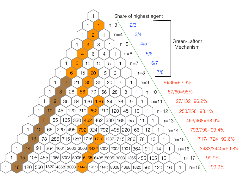
Corollary 1 allows us to compute the allocation probabilities of the highest valuation agent using the Pascal triangle in Figure 1. Each row (starting with the second row) represents a particular value of $n$ , starting with $n=3$ in the second row. By Corollary 1, $\ell=2$ if $n<8$ , $\ell\in\{2,4\}$ if $n=8$ , and $\ell=\lfloor\frac{n+1}{2}\rfloor_{e}$ if $n>9$ . In each row of the Pascal triangle, the entries are $C(n-2,0),C(n-2,1),\ldots,C(n-2,n-2)$ . Now, the value $C(n-2,\ell-1)$ is highlighted in the orange (lighter shaded) cell of each row. ⁸⁸ 8 The values in the brown (darker shaded) cells correspond to the entries of the Green-Laffont allocation rule. The probability of the highest valuation agent is then easily computed from this and the value of $\ell$ as: $\frac{C(n-2,\ell-1)+1}{C(n-2,\ell-1)+\ell}$ , which is shown to the right of the Pascal triangle.

Note that for $n\geq 14$ , the object is allocated to the highest valuation agent with at least 99% probability. The Green-Laffont allocation rule will require at least 100 agents to achieve such probability for the highest valuation agent.

Refer to caption — Figure 1: The r-optimal allocation rule

3.3 Participation Constraints

We now show that a strong form of participation constraint is satisfied by a class of ranking mechanisms, including the r-optimal mechanism in Theorem 1.

Definition 5

A mechanism $(f,\mathbf{p})$ is ex-post individually rational if for every $i\in N$ and for every $\mathbf{v}$ , we have

v_{i}f_{i}(\mathbf{v})-p_{i}(\mathbf{v})\geq 0.

The ex-post notion of participation constraint is appropriate in our prior-free model. Notice that, unlike the model in Cramton et al. (1987), our model does not have any property rights defined for the agents. ⁹⁹ 9 We discuss the results in Cramton et al. (1987) in details in Section 5. Hence, we assume that the outside option of each agent is zero. In that sense, even though our participation constraints are ex-post, they only ensure non-negative payoff from participation. On the other hand, the participation constraints in Cramton et al. (1987) is interim but because of the property rights structure, they ensure larger interim payoffs to agents.

We prove below that a class of mechanisms using two-step ranking allocation rules satisfy ex-post individual rationality. For $n\geq 8$ , the two extremes of this class are the Green-Laffont mechanism and our r-optimal mechanism in Theorem 1.

Theorem 2

Suppose $f$ is a two-step ranking allocation rule defined by $(\pi_{1},\ell)$ , where $2\ell\leq n+1$ . If $(f,\mathbf{p})$ is a satisfactory mechanism, then it is ex-post individually rational.

The r-optimal allocation rule in Theorem 1 satisfies the sufficient condition identified in Theorem 2.

Corollary 2

Suppose $f$ is the r-optimal allocation rule identified in Theorem 1. If $(f,\mathbf{p})$ is a satisfactory mechanism, then it is ex-post individually rational.

Proof: By Corollary 1, the r-optimal allocation rule in Theorem 1 satisfies $2\ell\leq n+1$ . By Theorem 2, the claim follows. $\blacksquare{}$

We compute the payments in the mechanisms discussed in Theorem 2. While the general payment formula for a satisfactory mechanism is quite complicated (see Theorem 4), the payment formula for the mechanisms in Theorem 2 is easier to express.

Notation. For any pair of positive integers, $K,K^{\prime}$ with $K\geq K^{\prime}$ ,

\psi(K^{\prime},K):=K^{\prime}\times(K^{\prime}+1)\times\ldots\times K

Proposition 2

Suppose $(f,\mathbf{p})$ is a satisfactory mechanism, where $f$ is a two-step ranking allocation rule defined by $(\pi_{1},\ell)$ with $\pi_{1}+(\ell-1)\pi_{2}=1$ . For any valuation profile $\mathbf{v}$ with $v_{1}>v_{2}>\ldots>v_{n}>0$ , we have

•

if $i=1$ , then

p_{i}(\mathbf{v})=-\frac{\pi_{2}}{(\ell-1)!}\Big[\sum_{k=1}^{\ell-1}(-1)^{k}(k-1)!\psi(n-\ell,n-k-1)v_{k+1}\Big].

•

if $i\in\{2,\ldots,\ell\}$ , then

p_{i}(\mathbf{v})=-\frac{\pi_{2}}{(\ell-1)!}\Big[\sum_{k=2}^{i-1}(-1)^{k}(k-1)!\psi(n-\ell,n-k-1)v_{k}+\sum_{k=i}^{\ell-1}(-1)^{k}(k-1)!\psi(n-\ell,n-k-1)v_{k+1}\Big].

•

if $i>\ell$ , then

p_{i}(\mathbf{v})=-\frac{\pi_{2}}{(\ell-1)!}\Big[\sum_{k=2}^{\ell-1}(-1)^{k}(k-1)!\psi(n-\ell,n-k-1)v_{k}+(-1)^{\ell}(\ell-1)!v_{\ell}\Big].

In any two step ranking allocation rule $(\pi_{1},\ell)$ , at a valuation profile $\mathbf{v}$ with $v_{1}>v_{2}>\ldots>v_{n}>0$ , an agent $i$ with $i>\ell$ gets the object with zero probability - call such agents losing agents. According to the payment formula computed in Proposition 2, losing agents receive some payments. Theorem 2 shows that losing agents receive non-negative payment if $2\ell\leq n+1$ . Hence, participation constraints are satisfied for losing agents in such class of mechanisms. For two step ranking allocation rules, where $2\ell>n+1$ , it is possible that losing agents may be asked to pay, violating their participation constraint.

3.4 Pareto Optimal Ranking Mechanisms

We now discuss an alternate prior-free notion of comparing mechanisms, where we compare mechanisms at every valuation profile in term of total social welfare. Informally, a satisfactory mechanism $\mathcal{M}$ dominates another satisfactory mechanism $\mathcal{M}^{\prime}$ if $\mathcal{M}$ generates as much total welfare as $\mathcal{M}^{\prime}$ in every profile of valuations and strictly higher in some profile of valuations. A satisfactory mechanism is Pareto optimal if it is not dominated by any other satisfactory mechanism.

It is a relatively weak notion to compare mechanisms - for instance, it may be that a Pareto optimal mechanism is dominated by another satisfactory mechanism at a positive measure of valuation profiles. Two satisfactory mechanisms may not even be comparable using this notion.

We adapt the notion of Pareto optimality to the class of ranking mechanisms.

Definition 6

A ranking allocation rule $f$ is r-Pareto optimal if (i) $f$ is satisfactorily implementable and (ii) there does not exist another ranking allocation rule $f^{\prime}$ such that $f^{\prime}$ is satisfactorily implementable and at every valuation profile $\mathbf{v}$ , we have

\sum_{i\in N}v_{i}f^{\prime}_{i}(\mathbf{v})\geq\sum_{i\in N}v_{i}f_{i}(\mathbf{v}),

with strict inequality holding at some $\mathbf{v}$ .

A ranking mechanism $(f,\mathbf{p})$ is r-Pareto optimal if (i) $(f,\mathbf{p})$ is a satisfactory mechanism and (ii) $f$ is r-Pareto optimal.

We first show that the GL allocation rule is an r-Pareto optimal allocation rule.

Theorem 3

The GL allocation rule is an r-Pareto optimal allocation rule. Moreover, it is the unique r-Pareto optimal allocation rule satisfying $\pi_{3}=\ldots=\pi_{n}=0$ .

Theorem 3 gives a foundation for the GL mechanism. Among all ranking mechanisms that only allocate the object to top-two agents, the GL mechanism is the unique r-Pareto optimal mechanism. As we show in the next result, if $n\leq 8$ , the GL mechanism is the unique r-Pareto optimal mechanism, but there are other r-Pareto optimal mechanisms if the number of agents is greater than $8$ . In particular, our r-optimal mechanism is always r-Pareto optimal.

Proposition 3

For $n\leq 8$ , the GL allocation rule is the unique r-Pareto optimal allocation rule. For $n>8$ , the unique r-optimal allocation rule identified in Theorem 1 is also r-Pareto optimal. Further, for any arbitrary r-Pareto optimal allocation rule $(\pi_{1},\ldots,\pi_{n})$ , we have

1-1/n\leq\pi_{1}\leq\pi_{1}^{*},

where $\pi_{1}^{*}$ is as defined in Theorem 1.

4 Satisfactory Implementability

In this section, we provide a characterization that drives all our main results. In particular, we provide a complete characterization of allocation rules which can be satisfactorily implemented. Besides the technical aspect, there are other reasons why such a characterization is useful: (1) it provides a recipe for carrying out such analysis of satisfactory mechanisms in other models and (2) it showcases the rich but complex class of non-ranking mechanisms that are satisfactory, thus, highlighting the salience of ranking mechanisms.

Before stating the characterization, we remind the reader about the following characterization of DSIC mechanisms by Myerson. ¹⁰¹⁰ 10 The characterization in Myerson is for Bayesian incentive compatible mechanisms. However, it is straightforward to extend it to DSIC mechanisms.

Lemma 1 (Myerson (1981))

A mechanism $(f,\mathbf{p})$ is DSIC if and only if

•

Montonicity of $f$ . for every $i\in N$ , for every $v_{-i}\in V^{n-1}$ , and for every $v_{i},v^{\prime}_{i}\in V$ with $v_{i}>v^{\prime}_{i}$ , we have

$f_{i}(v_{i},v_{-i})\geq f_{i}(v^{\prime}_{i},v_{-i}).$
•

Revenue Equivalence. for every $i\in N$ , for every $v_{-i}\in V^{n-1}$ , and for every $v_{i}\in V$ , we have

$p_{i}(v_{i},v_{-i})=p_{i}(0,v_{-i})+v_{i}f_{i}(v_{i},v_{-i})-\int_{0}^{v_{i}}f_{i}(x_{i},v_{-i})dx_{i}.$

For any mechanism $M\equiv(f,\mathbf{p})$ , we define $\mathcal{U}^{M}_{i}(\mathbf{v})$ as the net utility of agent $i$ at valuation profile $\mathbf{v}$ :

\mathcal{U}^{M}_{i}(\mathbf{v})=v_{i}f_{i}(\mathbf{v})-p_{i}(\mathbf{v}).

A consequence of the Myersonian characterization of DSIC is the following characterization of DSIC and budget-balanced mechanisms.

Proposition 4

A mechanism $M\equiv(f,\mathbf{p})$ is DSIC and budget-balanced if and only if

1.

for every $i\in N$ , for every $v_{-i}\in V^{n-1}$ , and for every $v_{i},v^{\prime}_{i}\in V$ with $v_{i}>v^{\prime}_{i}$ we have

$\displaystyle f_{i}(v_{i},v_{-i})\geq f_{i}(v^{\prime}_{i},v_{-i}).$

for every $i\in N$ , for every $v_{-i}\in V^{n-1}$ , for every $v_{i}\in V$ , we have

\displaystyle\mathcal{U}_{i}^{M}(v_{i},v_{-i})

\displaystyle=\mathcal{U}_{i}^{M}(0,v_{-i})+\int_{0}^{v_{i}}f_{i}(x_{i},v_{-i})dx_{i}.

for every $\mathbf{v}\equiv(v_{1},\ldots,v_{n})\in V^{n}$ ,

\displaystyle\sum_{i\in N}\mathcal{U}_{i}^{M}(0,v_{-i})

\displaystyle=\sum_{i\in N}\big[v_{i}f_{i}(\mathbf{v})-\int_{0}^{v_{i}}f_{i}(x_{i},v_{-i})dx_{i}\big].

Proof: From Lemma 1, (1) and (2) are equivalent to DSIC. For (3), note that budget-balance of a mechanism $M\equiv(f,\mathbf{p})$ requires that for all $\mathbf{v}\equiv(v_{1},\ldots,v_{n})\in V^{n}$ , we must have

\displaystyle\sum_{i\in N}\mathcal{U}^{M}_{i}(\mathbf{v})

\displaystyle=\sum_{i\in N}v_{i}f_{i}(\mathbf{v}).

Using (2), we conclude that a DSIC mechanism is budget-balanced if and only if for all $\mathbf{v}\equiv(v_{1},\ldots,v_{n})\in V^{n}$ ,

\displaystyle\sum_{i\in N}\mathcal{U}_{i}^{M}(0,v_{-i})+\sum_{i\in N}\int_{0}^{v_{i}}f_{i}(x_{i},v_{-i})dx_{i}

\displaystyle=\sum_{i\in N}v_{i}f_{i}(\mathbf{v}).

Equivalently, a DSIC mechanism $M\equiv(f,\mathbf{p})$ is budget-balanced if and only if for all $\mathbf{v}\equiv(v_{1},\ldots,v_{n})\in V^{n}$ ,

\displaystyle\sum_{i\in N}\mathcal{U}_{i}^{M}(0,v_{-i})

\displaystyle=\sum_{i\in N}\big[v_{i}f_{i}(\mathbf{v})-\int_{0}^{v_{i}}f_{i}(x_{i},v_{-i})dx_{i}\big].

$\blacksquare{}$

Our main characterization, like Myerson’s characterization, provides a way to separate out the allocation rule and the payment rule in a satisfactory mechanism. While Myerson does not impose budget-balance, our result shows that this separation continues to hold even if we impose budget-balance.

Fix an allocation rule $f$ . If $f$ is monotone (in the sense of Lemma 1), then we can immediately define a payment scheme $\mathbf{p}$ that makes $(f,\mathbf{p})$ DSIC as follows: for every $i\in N$ and for every $\mathbf{v}$ , set

p_{i}(\mathbf{v})=v_{i}f_{i}(\mathbf{v})-\int_{0}^{v_{i}}f_{i}(x_{i},v_{-i})dx_{i}.

Note that $p_{i}(0,v_{-i})=0$ for all $i$ and for all $v_{-i}$ in this mechanism. We call a mechanism defined from such a payment scheme as the elementary mechanism corresponding to a monotone $f$ . It can be easily verified that if $f$ is the efficient allocation rule, then the corresponding elementary mechanism is the Vickrey auction.

For every valuation profile $\mathbf{v}$ , define for every $i\in N$ , the payment of agent $i$ in the elementary mechanism corresponding to a monotone $f$ as:

R^{f}_{i}(\mathbf{v}):=v_{i}f_{i}(\mathbf{v})-\int_{0}^{v_{i}}f_{i}(x_{i},v_{-i})dx_{i}.

Then,

R^{f}(\mathbf{v}):=\sum_{i\in N}R^{f}_{i}(\mathbf{v}),

denotes the total revenue collected at valuation profile $\mathbf{v}$ in the elementary mechanism corresponding to $f$ .

We will provide necessary and sufficient conditions on $f$ for it to be satisfactorily implementable. These conditions are given in terms of revenue collected from the elementary mechanism corresponding to $f$ at various valuation profiles.

At any valuation profile $\mathbf{v}$ , define $N^{0}_{\mathbf{v}}:=\{i\in N:v_{i}=0\}$ . Given any valuation profile $\mathbf{v}$ , for any $T\subseteq N$ , we denote by $(0_{T},v_{-T})$ the valuation profile where all the agents in $T$ have zero valuation and each agent $i\notin T$ has valuation $v_{i}$ .

Definition 7

An allocation rule $f$ is residually balanced if for every $\mathbf{v}$ such that $N^{0}_{\mathbf{v}}=\emptyset$ , we have

\displaystyle\sum_{T\subseteq N}(-1)^{|T|}~R^{f}(0_{T},v_{-T})

\displaystyle=0.

(1)

Residual balancedness is a technical combinatorial condition on an allocation rule. We show that for a symmetric and monotone allocation rule residual balancedness is necessary and sufficient for satisfactory implementability.

Theorem 4

A symmetric allocation rule $f$ is satisfactorily implementable if and only if it is (a) monotone and (b) residually balanced.

Further, if $f$ is satisfactorily implementable, then there is a unique $\mathbf{p}$ such that $(f,\mathbf{p})$ is a satisfactory mechanism. Such a unique $\mathbf{p}$ is defined as follows: for all $\mathbf{v}\in V^{n}$ , for all $i\in N$ ,

	$\displaystyle p_{i}(\mathbf{v})$	$\displaystyle=-\frac{1}{\|N^{0}_{\mathbf{v}}\|}\sum_{T\subseteq N:N^{0}_{\mathbf{v}}\subseteq T}\frac{(-1)^{\|T\setminus N^{0}_{\mathbf{v}}\|}}{C(\|T\|,\|N^{0}_{\mathbf{v}}\|)}R^{f}(0_{T},v_{-T})~\qquad~\text{if $i\in N^{0}_{\mathbf{v}}$}$
	$\displaystyle p_{i}(\mathbf{v})$	$\displaystyle=R^{f}_{i}(\mathbf{v})-\frac{1}{\|N^{0}_{\mathbf{v}}\|+1}\sum_{T\subseteq N:(N^{0}_{\mathbf{v}}\cup\{i\})\subseteq T}\frac{(-1)^{\|T\setminus N^{0}_{\mathbf{v}}\|-1}}{C(\|T\|,(\|N^{0}_{\mathbf{v}}\|+1))}R^{f}(0_{T},v_{-T})~\qquad~\text{if $i\notin N^{0}_{\mathbf{v}}$}$

The condition in Theorem 4 looks very similar to the cubical array lemma in Walker (1980). While the cubical array lemma applies to only efficient allocation rule, our characterization is for any allocation rule. Theorem 2 in Yenmez (2015) characterizes ex-post incentive compatible and budget-balanced mechanisms. ¹¹¹¹ 11 His solution concept is ex-post incentive compatibility because he looks at a setting that can potentially allow for interdependent valuations. His characterization is a characterization of DSIC and budget-balanced mechanisms, and hence, still uses transfers. On the other hand, the advantage of our characterization is that it gives necessary and sufficient condition on the allocation rule to be satisfactorily implementable. Thus, we are able to separate out allocation rule and payments for analyzing budget-balanced mechanisms.

The proof of Theorem 4 is in the Appendix. It is notationally quite complex. Here, we illustrate the idea of the necessity part with an example of three agents: $N=\{1,2,3\}$ . Let $f$ be a symmetric, monotone, and satisfactorily implementable allocation rule. Then, there is a $\mathbf{p}$ such that $(f,\mathbf{p})$ is a satisfactory mechanism. Consider a valuation profile $\mathbf{v}\equiv(0,0,0)$ . By BB and symmetry, we get $p_{1}(\mathbf{v})=p_{2}(\mathbf{v})=p_{3}(\mathbf{v})=0$ . Now, consider a valuation profile $\mathbf{v}\equiv(v_{1},0,0)$ . By Lemma 1,

p_{1}(\mathbf{v})=p_{1}(0,0,0)+R_{1}^{f}(\mathbf{v})=R_{1}^{f}(\mathbf{v}).

Note that $R^{f}(\mathbf{v})=R^{f}_{1}(\mathbf{v})$ . By symmetry $p_{2}(\mathbf{v})=p_{3}(\mathbf{v})$ . Hence, by BB and symmetry,

0=p_{1}(\mathbf{v})+2p_{2}(\mathbf{v})=2p_{2}(\mathbf{v})+R^{f}(\mathbf{v}).

This implies that

p_{2}(v_{1},0,0)=-\frac{1}{2}R^{f}(v_{1},0,0).

Now, consider a valuation profile $\mathbf{v}\equiv(v_{1},v_{2},0)$ . Using BB and Lemma 1, and following the above arguments, we get

	$\displaystyle p_{1}(\mathbf{v})=p_{1}(0,v_{2},0)+R^{f}_{1}(\mathbf{v})=-\frac{1}{2}R^{f}(0,v_{2},0)+R^{f}_{1}(\mathbf{v})$
	$\displaystyle p_{2}(\mathbf{v})=p_{2}(v_{1},0,0)+R^{f}_{2}(\mathbf{v})=-\frac{1}{2}R^{f}(v_{1},0,0)+R^{f}_{2}(\mathbf{v})$

Adding these two with $p_{3}(\mathbf{v})$ and using BB, we get

p_{3}(v_{1},v_{2},0)=\frac{1}{2}\Big(R^{f}(v_{1},0,0)+R^{f}(0,v_{2},0)\Big)-R^{f}(v_{1},v_{2},0).

Finally, consider the valuation profile $(v_{1},v_{2},v_{3})$ with $v_{1},v_{2},v_{3}>0$ . Again, using Lemma 1, we get

	$\displaystyle p_{1}(\mathbf{v})=p_{1}(0,v_{2},v_{3})+R^{f}_{1}(\mathbf{v})=\frac{1}{2}\Big(R^{f}(0,v_{2},0)+R^{f}(0,0,v_{3})\Big)-R^{f}(0,v_{2},v_{3})+R^{f}_{1}(\mathbf{v})$
	$\displaystyle p_{2}(\mathbf{v})=p_{2}(v_{1},0,v_{3})+R^{f}_{2}(\mathbf{v})=\frac{1}{2}\Big(R^{f}(v_{1},0,0)+R^{f}(0,0,v_{3})\Big)-R^{f}(v_{1},0,v_{3})+R^{f}_{2}(\mathbf{v})$
	$\displaystyle p_{3}(\mathbf{v})=p_{3}(v_{1},v_{2},0)+R^{f}_{2}(\mathbf{v})=\frac{1}{2}\Big(R^{f}(0,v_{2},0)+R^{f}(v_{1},0,0)\Big)-R^{f}(v_{1},v_{2},0)+R^{f}_{3}(\mathbf{v})$

Adding and using BB, we get

R^{f}(v_{1},v_{2},v_{3})-R^{f}(v_{1},v_{2},0)-R^{f}(0,v_{2},v_{3})-R^{f}(v_{1},0,v_{3})+R^{f}(v_{1},0,0)+R^{f}(0,v_{2},0)+R^{f}(0,0,v_{3})=0,

which is the residual balancedness condition. The sufficiency can be shown using the explicit form of payment functions hidden in these calculations. In summary, residual balancedness allows a recursive calculation of payments at all valuation profiles so that budget-balance holds.

5 Relation to the Literature

The impossibility of achieving efficiency, dominant strategy incentive compatibility, and budget-balance was first shown by Green and Laffont (1979), which also contains a lot of discussions on achieving second-best using non-efficient but DSIC and budget-balanced mechanisms. This includes the Green-Laffont mechanism that we discuss. Though, they focussed attention on public good problems and gave sketches of the Green-Laffont mechanism we discuss, they clearly anticipated the mechanism as well as many environments beyond the public good problem where the impossibility result would hold. Gary-Bobo and Jaaidane (2000) contains an extensive discussion on this - they also formally define the Green-Laffont mechanism and study its statistical and strategic properties in the public good problem.

This impossibility result started a long literature on how to overcome it. We classify them in several categories and discuss some relevant ones. Most of the literature we discuss concern with private good allocation among several buyers. There are parallel literature on bilateral trading and public good provision that we do not discuss.

Domain identification. Classic revenue equivalence results imply that every efficient and DSIC mechanism must be a Groves mechanism (Green and Laffont, 1977; Holmström, 1979). The Green-Laffont impossibility result essentially implies that no Groves mechanism can balance budget in many settings - though their focus is mainly of public good problems. In the public good context, Laffont and Maskin (1980) consider differentiable mechanisms and show that existence of a DSIC, BB, and efficient mechanism is equivalent to solving a system of differential equations. In the same model, Walker (1980) identifies domains (of utility functions of agents) where impossibilities exist - he restricts attention to continuous mechanisms. As corollary of their results, they identify form of utility functions of agents where possibility or impossibility result exists. Hurwicz and Walker (1990) extend the Green-Laffont impossibility to pure exchange economies. These papers are mainly focused on identifying domains where the negative result of Green and Laffont persists.

But there are settings where DSIC, BB, and efficient mechanisms exist. Suijs (1996) is a good example of a domain where Groves mechanisms that balance the budget exists - he discusses a sequencing problem. In the context of multi-object assignment, a recent contribution is Mitra and Sen (2010). This paper identifies domains of multi-object auctions where the Green-Laffont impossibility can be overcome.

Bayesian incentive compatibility. One way to get around the Green-Laffont impossibility is to consider the weaker solution concept of Bayesian incentive compatibility. Arrow (1979); d’Aspremont and Gérard-Varet (1979) construct Bayesian incentive compatible, efficient, and budget-balanced mechanism, now known as the dAGV mechanism, that work in a variety of settings. The dAGV mechanisms fail to be interim individually rational in many settings. In an unpublished paper, Fudenberg et al. (1995) extend this result in the following sense - for every Bayes-Nash implementable allocation rule, there exists a Bayesian incentive compatible and budget-balanced mechanism using this allocation rule. Like in the dAGV mechanism, such budget-balanced mechanisms need not satisfy interim individual rationality. Rahman (2011) gives a characterization of Bayesian (and ex-post) incentive compatible and budget-balanced mechanisms in a very general framework.

In a seminal paper, Cramton et al. (1987) show that efficient, Bayesian incentive compatible, budget-balanced mechanisms satisfying interim individual rationality is possible in a single object allocation problem. ¹²¹² 12 They consider a problem where agents have property rights over the object, and stronger form of interim individual rationality is satisfied by their mechanism. However, their results can still be applied to our problem if we assume equal property rights to all the agents. The possibility result in our problem using Bayesian incentive compatibility is in sharp contrast to the impossibility results known in bilateral trading problems like in Myerson and Satterthwaite (1983).

Unlike Cramton et al. (1987), we focus on DSIC mechanisms, and our mechanism is not efficient. Naturally, the mechanism in Cramton et al. (1987) require a lot of prior information. Our mechanism is prior-free and satisfies ex-post individually rationality. Thus, we illustrate a prior-free way of approximately achieving the possibility result in Cramton et al. (1987).

Redistribution mechanisms. The prior-free approach of mechanism design using DSIC mechanisms have been popular in algorithmic game theory literature in computer science. Restricting attention to efficient mechanisms, which means restricting attention to Groves mechanisms, several papers relax budget-balance and show how best to redistribute the surplus revenue. The measure of efficiency of redistribution is worst-case in these papers. One of the earliest papers to do this is Cavallo (2006), who studied this problem in our setting (single object allocation). He showed that remarkable Groves mechanisms exist that can redistribute large fraction of Vickrey auction payments using Groves mechanisms. Moulin (2009) and Guo and Conitzer (2009) derive optimal redistribution mechanisms in the multi-unit allocation setting where agents demand exactly one unit - their mechanisms are identical and discovered independently. ¹³¹³ 13 Several papers related to this theme have also appeared - see for instance, Apt et al. (2008) and Moulin (2010). As the number of agents increase, like our mechanism, their Groves mechanisms can redistribute large fraction of Vickrey auction revenue among agents. The main difference from these papers and ours is budget-balance. Since these papers do not impose budget-balance, the actual budget imbalance in these mechanisms can be high in various valuation profiles. On the other hand, like in Cramton et al. (1987), budget-balance is a constraint in our problem. Hence, unlike these papers, we work with mechanisms outside the Groves class. Our results show that we can achieve excellent levels of efficiency (99% with at least 14 agents) using DSIC and budget-balanced mechanisms.

Beyond Groves mechanisms. While most of the literature seems to have either weakened DSIC to Bayesian incentive compatibility or relaxed the budget-balanced criteria while working with efficient and DSIC mechanisms (Groves mechanisms), there is very little literature on exploring the limits of DSIC and budget-balanced mechanisms. We do this for the case of single object allocation problem. One of the problems with exploring non-Groves mechanisms is that we search over the space of allocation rules and payment rules - Groves mechanisms pin down the allocation rule to be the efficient allocation rule. A non-efficient allocation rule can achieve better social welfare redistribution is well known - see for instance examples in Laffont and Maskin (1980) and a more computational analysis in de Clippel et al. (2009). Sprumont (2013) consider Pareto-undominated mechanisms by considering DSIC and non-efficient mechanisms, though his mechanisms are not budget-balanced. Faltings (2005) and Guo et al. (2011) consider variants of Green-Laffont mechanisms discussed in Green and Laffont (1979) and show some worst-case results, but they do not consider the general class of DSIC and budget-balanced mechanisms that we analyze. Hashimoto (2015) discusses a non-ranking satisfactory mechanism and provides several axiomatization his mechanism.

Another possibility is to consider priors and design the expected welfare maximizing DSIC and budget-balanced mechanism for allocating an object. This is similar to the expected revenue maximizing question in Myerson (1981), but significantly more complicated. Restricting attention to the case of two agents and deterministic mechanisms, Drexl and Kleiner (2015) derive the optimal expected welfare maximizing DSIC and budget-balanced mechanism. Shao and Zhou (2013) do the same analysis for two agents but without requiring budget-balance. These papers illustrate difficulty in extending such analysis to more than two agents. In that sense, we provide a prior-free method of measuring welfare of mechanisms which turns out to be tractable for any number of agents.

6 Conclusion

This paper provides a novel DSIC, budget-balanced, symmetric, and ex-post individually rational mechanism to allocate a single unit of a resource. The mechanism converges to efficiency with moderately high number of agents. Further, the mechanism can be viewed as a generalization of the Green-Laffont mechanism. From a methodological standpoint, we provide several key insights on how to analyze DSIC and budget-balanced mechanisms, and propose a tractable class of mechanisms that we call ranking mechanisms.

While we carry out this analysis for allocating a single unit of resource, we feel that the ideas in this paper can be pushed in other models of mechanism design where budget-balance is a constraint. Further, an indirect implementation of our mechanism will significantly improve the practicality of our proposed mechanism.

From a broader perspective, our results quantify the impossibility on designing DSIC, budget-balanced, and efficient mechanisms in the single object allocation problem. It shows that even though impossibility exists, it is really thin. Thus, the possibility results with Bayesian incentive compatibility (Cramton et al., 1987) or approximate possibility results with relaxed budget-balanced constraints (Guo and Conitzer, 2009; Moulin, 2009) can also be approximately achieved with DSIC and budget-balanced mechanisms.

Appendix: Omitted Proofs

This section contains all the missing proofs. We first prove our workhorse result - Theorem 4. Once this result is proved, we use it to prove Proposition 1. Then, we proceed to prove our two main results - Theorem 3 and Theorem 1. Then, we prove our individual rationality result - Theorem 2.

Notations. We will need some extra notations. At every valuation profile $\mathbf{v}$ and for every $k\in N$ , we denote by $v_{(k)}$ the valuation of every agent in $\mathbf{v}[k]$ . Note that for some $k\in N$ , it is possible that $\mathbf{v}[k]=\emptyset$ , in which case $v_{(k)}$ is defined to be $0$ . For any $j\in N$ , let the cardinality of the set $\cup_{h=1}^{j}\mathbf{v}[h]$ be $L_{j}$ .

We illustrate these notations with an example. Suppose $N=\{1,\ldots,8\}$ . Consider a valuation profile $\mathbf{v}$ such that $\mathbf{v}[1]=\{1,2\}$ , $\mathbf{v}[2]=\{3,4,5,6\}$ , and $\mathbf{v}[3]=\{7,8\}$ . Then, $L_{1}=2,L_{2}=6,L_{3}=8$ . According to a ranking allocation rule with probabilities $(\pi_{1},\ldots,\pi_{8})$ , agents $1$ and $2$ share $\pi_{1}+\pi_{2}$ equally, agents $3,4,5,6$ share $\pi_{3}+\pi_{4}+\pi_{5}+\pi_{6}$ equally and agents $7$ and $8$ share $\pi_{7}+\pi_{8}$ equally. In other words, for every $j\in N$ , agents in $\mathbf{v}[j]$ share equally the probabilities

\pi_{L_{j-1}+1}+\ldots+\pi_{L_{j}},

where $L_{0}\equiv 0$ .

We begin by a lemma, which will be useful to all our proofs.

Lemma 2

Suppose $f$ is a ranking allocation rule. Then, $R^{f}$ is continuous.

Proof: For any $\mathbf{v}$ , we know that

R^{f}(\mathbf{v})=\sum_{i\in N}v_{i}f_{i}(\mathbf{v})-\sum_{i\in N}\int_{0}^{v_{i}}f_{i}(x_{i},v_{-i})dx_{i}.

We now do the proof in two steps. Assume that the allocation probabilities of the ranking allocation rule are $\pi_{1}\geq\pi_{2}\geq\ldots\geq\pi_{n}$ .

Step 1. In this step, we show that for every $i\in N$ , the expression $\int_{0}^{v_{i}}f_{i}(x_{i},v_{-i})dx_{i}$ is continuous in $\mathbf{v}$ . Fix a valuation profile $\mathbf{v}$ . Consider agent $i$ and suppose $i\in\mathbf{v}[j]$ . Hence, $v_{i}\equiv v_{(j)}$ for some $j$ . Then, using the definition of the ranking allocation rule, we note that

	$\displaystyle\int_{0}^{v_{i}}f_{i}(x_{i},v_{-i})dx_{i}$	$\displaystyle=\int_{0}^{v_{(j)}}f_{i}(x_{i},v_{-i})dx_{i}$
		$\displaystyle=\pi_{L_{j}}(v_{(j)}-v_{(j+1)})+\pi_{L_{j+1}}(v_{(j+1)}-v_{(j+2)})+\ldots$
		$\displaystyle=\sum_{h\geq j}\pi_{L_{h}}(v_{(h)}-v_{(h+1)}).$

To establish continuity, we look at a valuation profile $\mathbf{v}^{\prime}$ which is arbitrarily close to $\mathbf{v}$ , and $\mathbf{v}^{\prime}$ and $\mathbf{v}$ differ in valuation of only agent $k$ - it is enough to look at valuation profiles that differ in one component. Suppose $k\in\mathbf{v}[\ell]$ . If $\ell<j$ , then there is nothing to prove since the above summation is unchanged from $\mathbf{v}$ to $\mathbf{v}^{\prime}$ . Hence, assume $\ell\geq j$ . Since $\mathbf{v}^{\prime}$ is arbitrarily close to $\mathbf{v}$ , it must be that $k\in\mathbf{v}^{\prime}[\ell]$ (this happens if $v_{k}^{\prime}>v_{k}$ ) or $k\in\mathbf{v}^{\prime}[\ell+1]$ (this happens if $v_{k}^{\prime}<v_{k}$ ). Indeed, since $\mathbf{v}^{\prime}$ is arbitrarily close to $\mathbf{v}$ , it must be that $\{k\}=\mathbf{v}^{\prime}[\ell+1]$ or $\{k\}=\mathbf{v}^{\prime}[\ell]$ . We consider both the cases separately. We denote the cardinality of the set $\cup_{h=1}^{r}\mathbf{v}^{\prime}[h]$ by $L_{r}^{\prime}$ for all $r$ . Note that if $\{k\}=\mathbf{v}[\ell]$ (i.e., if $k$ is the only element in $\mathbf{v}[\ell]$ ), then $L_{r}=L_{r}^{\prime}$ for all $r$ . As a result,

	$\displaystyle\int_{0}^{v_{i}^{\prime}}f_{i}(x_{i},v_{-i}^{\prime})dx_{i}$	$\displaystyle=\sum_{h\geq j}\pi_{L_{h}^{\prime}}(v_{(h)}^{\prime}-v_{(h+1)}^{\prime})$
		$\displaystyle\rightarrow\sum_{h\geq j}\pi_{L_{h}}(v_{(h)}-v_{(h+1)})$
		$\displaystyle=\int_{0}^{v_{i}}f_{i}(x_{i},v_{-i})dx_{i}$

So, the claim is true. Hence, we assume $|\mathbf{v}[\ell]|>1$ . Now, consider the following two cases.

Case 1-a. Suppose $\{k\}=\mathbf{v}^{\prime}[\ell]$ . Since $|\mathbf{v}[\ell]|>1$ , $v^{\prime}_{(\ell)}=v^{\prime}_{k}\rightarrow v_{k}=v_{(\ell)}=v^{\prime}_{(\ell+1)}$ . Then, $L^{\prime}_{r}=L_{r}$ for all $r<\ell$ and $L^{\prime}_{r}=L_{r-1}$ for all $r>\ell$ . Further, $v^{\prime}_{(r)}=v_{(r)}$ for all $r<\ell$ and $v^{\prime}_{(r)}=v_{(r-1)}$ for all $r>\ell$ . As a result,

	$\displaystyle\int_{0}^{v^{\prime}_{i}}f_{i}(x_{i},v^{\prime}_{-i})dx_{i}$	$\displaystyle=\sum_{h\geq j}\pi_{L^{\prime}_{h}}(v^{\prime}_{(h)}-v^{\prime}_{(h+1)})$
		$\displaystyle=\sum_{h=j}^{\ell-1}\pi_{L^{\prime}_{h}}(v^{\prime}_{(h)}-v^{\prime}_{(h+1)})+\pi_{L^{\prime}_{\ell}}(v^{\prime}_{(\ell)}-v^{\prime}_{(\ell+1)})+\sum_{h\geq\ell+1}\pi_{L^{\prime}_{h}}(v^{\prime}_{(h)}-v^{\prime}_{(h+1)})$
		$\displaystyle\rightarrow\sum_{h=j}^{\ell-1}\pi_{L_{h}}(v_{(h)}-v_{(h+1)})+\sum_{h\geq\ell+1}\pi_{L_{h-1}}(v_{(h-1)}-v_{(h)})$
		$\displaystyle=\sum_{h=j}^{\ell-1}\pi_{L_{h}}(v_{(h)}-v_{(h+1)})+\sum_{h\geq\ell}\pi_{L_{h}}(v_{(h)}-v_{(h+1)})$
		$\displaystyle=\int_{0}^{v_{i}}f_{i}(x_{i},v_{-i})dx_{i}.$

This shows that $\int_{0}^{v_{i}}f_{i}(x_{i},v^{\prime}_{-i})dx_{i}\rightarrow\int_{0}^{v_{i}}f_{i}(x_{i},v_{-i})dx_{i}$ as $v^{\prime}_{k}\rightarrow v_{k}$ .

Case 1-b. Suppose $\{k\}=\mathbf{v}^{\prime}[\ell+1]$ . Since $|\mathbf{v}[\ell]|>1$ , we have $v^{\prime}_{(\ell)}=v_{(\ell)}$ . This implies that $v^{\prime}_{(\ell+1)}=v^{\prime}_{k}\rightarrow v_{k}=v_{(\ell)}=v^{\prime}_{(\ell)}$ .

Here, we need to worry about the case $k=i$ . If $k=i$ , then $i\in\mathbf{v}^{\prime}[\ell+1]$ . Further, for every $r\geq\ell+1$ , we have $L^{\prime}_{r}=L_{r-1}$ and for every $r>\ell+1$ , we have $v^{\prime}_{(r)}=v_{(r-1)}$ .

	$\displaystyle\int_{0}^{v^{\prime}_{i}}f_{i}(x_{i},v^{\prime}_{-i})dx_{i}$	$\displaystyle=\sum_{h\geq\ell+1}\pi_{L^{\prime}_{h}}(v^{\prime}_{(h)}-v^{\prime}_{(h+1)})$
		$\displaystyle=\pi_{L^{\prime}_{\ell+1}}(v^{\prime}_{(\ell+1)}-v^{\prime}_{(\ell+2)})+\sum_{h>\ell+1}\pi_{L^{\prime}_{h}}(v^{\prime}_{(h)}-v^{\prime}_{(h+1)})$
		$\displaystyle\rightarrow\pi_{L_{\ell}}(v_{(\ell)}-v_{(\ell+1)})+\sum_{h>\ell+1}\pi_{L_{h-1}}(v_{(h-1)}-v_{(h)})$
		$\displaystyle=\sum_{h\geq\ell+1}\pi_{L_{h-1}}(v_{(h-1)}-v_{(h)})$
		$\displaystyle=\sum_{h\geq\ell}\pi_{L_{h}}(v_{(h)}-v_{(h+1)})$
		$\displaystyle=\int_{0}^{v_{i}}f_{i}(x_{i},v_{-i})dx_{i}.$

This shows that $\int_{0}^{v_{i}}f_{i}(x_{i},v^{\prime}_{-i})dx_{i}\rightarrow\int_{0}^{v_{i}}f_{i}(x_{i},v_{-i})dx_{i}$ as $v^{\prime}_{i}\rightarrow v_{i}$ .

A similar proof works if $k\neq i$ . Then, $L^{\prime}_{r}=L_{r}$ for all $j<\ell$ and $L^{\prime}_{r}=L_{r-1}$ for all $r>\ell$ . Further, $v^{\prime}_{(r)}=v_{(r)}$ for all $r<\ell$ and $v^{\prime}_{(r)}=v_{(r-1)}$ for all $r>\ell$ . As a result,

	$\displaystyle\int_{0}^{v^{\prime}_{i}}f_{i}(x_{i},v^{\prime}_{-i})dx_{i}$	$\displaystyle=\sum_{h\geq j}\pi_{L^{\prime}_{h}}(v^{\prime}_{(h)}-v^{\prime}_{(h+1)})$
		$\displaystyle=\sum_{h=j}^{\ell-1}\pi_{L^{\prime}_{h}}(v^{\prime}_{(h)}-v^{\prime}_{(h+1)})+\pi_{L^{\prime}_{\ell}}(v^{\prime}_{(\ell)}-v^{\prime}_{(\ell+1)})+\sum_{h\geq\ell+1}\pi_{L^{\prime}_{h}}(v^{\prime}_{(h)}-v^{\prime}_{(h+1)})$
		$\displaystyle\rightarrow\sum_{h=j}^{\ell-1}\pi_{L_{h}}(v_{(h)}-v_{(h+1)})+\sum_{h\geq\ell+1}\pi_{L_{h-1}}(v_{(h-1)}-v_{(h)})$
		$\displaystyle=\sum_{h=j}^{\ell-1}\pi_{L_{h}}(v_{(h)}-v_{(h+1)})+\sum_{h\geq\ell}\pi_{L_{h}}(v_{(h)}-v_{(h+1)})$
		$\displaystyle=\int_{0}^{v_{i}}f_{i}(x_{i},v_{-i})dx_{i}.$

This again shows that $\int_{0}^{v_{i}}f_{i}(x_{i},v^{\prime}_{-i})dx_{i}\rightarrow\int_{0}^{v_{i}}f_{i}(x_{i},v_{-i})dx_{i}$ as $v^{\prime}_{k}\rightarrow v_{k}$ .

Step 2. Now, we argue that the summation $\sum_{i\in N}v_{i}f_{i}(\mathbf{v})$ is continuous. Fix a valuation profile $\mathbf{v}$ . Consider all the $j$ -th ranked valuation agents, $\mathbf{v}[j]$ , for some $j$ . Note that the total sum of welfare of agents in $\mathbf{v}[j]$ is

v_{(j)}\big(\pi_{L_{j-1}+1}+\ldots+\pi_{L_{j}}\big),

where $L_{0}\equiv 0$ . Hence, the total welfare of all agents is

\sum_{j=1}^{n}v_{(j)}\big(\pi_{L_{j-1}+1}+\ldots+\pi_{L_{j}}\big).

For any other valuation profile arbitrarily close to $\mathbf{v}$ , agents in $\mathbf{v}[j]$ will (a) have valuations arbitrarily close to $v_{(j)}$ and (b) their ranks (in the valuation profile) will be from $L_{j-1}+1$ to $L_{j}$ . As a result, their total welfare is arbitrarily close to

v_{(j)}\big(\pi_{L_{j-1}+1}+\ldots+\pi_{L_{j}}\big).

Applying this argument to every $j$ , we get that for any valuation arbitrarily close to $\mathbf{v}$ , the total welfare of agents is arbitrarily close to

\sum_{j=1}^{n}v_{(j)}\big(\pi_{L_{j-1}+1}+\ldots+\pi_{L_{j}}\big)=\sum_{i\in N}v_{i}f_{i}(\mathbf{v}).

Steps 1 and 2 show that $R^{f}$ is continuous in $\mathbf{v}$ . $\blacksquare{}$

Proof of Theorem 4

Proof: Suppose $f$ is a symmetric allocation rule which is satisfactorily implementable. This implies that there exists a symmetric $\mathbf{p}$ such that the mechanism $M\equiv(f,\mathbf{p})$ is satisfactory. By Proposition 4, $f$ is monotone. The remainder of the claims we do in steps.

Step 1. In this step, we show that for every $\mathbf{v}\in V^{n}$ such that $N^{0}_{\mathbf{v}}\neq\emptyset$ , we have for every $i\in N^{0}_{\mathbf{v}}$ ,

\displaystyle\mathcal{U}^{M}_{i}(\mathbf{v})

\displaystyle=\frac{1}{|N^{0}_{\mathbf{v}}|}\sum_{T\subseteq N:N^{0}_{\mathbf{v}}\subseteq T}\frac{(-1)^{|T\setminus N^{0}_{\mathbf{v}}|}}{C(|T|,|N^{0}_{\mathbf{v}}|)}R^{f}(0_{T},v_{-T}).

We show this using induction. If $|N^{0}_{\mathbf{v}}|=n$ , then budget-balance implies that $\sum_{i\in N}\mathcal{U}^{M}_{i}(\mathbf{v})=0$ . Symmetry implies that $\mathcal{U}^{M}_{j}(\mathbf{v})=\mathcal{U}^{M}_{k}(\mathbf{v})$ for all $j,k\in N$ at this valuation profile. Hence, $\mathcal{U}^{M}_{i}(\mathbf{v})=0$ for all $i\in N$ . Since $\mathbf{v}\equiv 0_{N}$ , we have $R^{f}(\mathbf{v})=0$ . Hence, the claim is true for $N^{0}=N$ .

Suppose the claim is true for all valuation profiles $\mathbf{\bar{v}}$ such that $|N^{0}_{\mathbf{\bar{v}}}|>|N^{0}_{\mathbf{v}}|$ . Let $K\equiv N^{0}_{\mathbf{v}}$ . Since $M$ is DSIC and budget-balanced, by Proposition 4, we get

	$\displaystyle R^{f}(\mathbf{v})$	$\displaystyle=\sum_{i\in N}\mathcal{U}^{M}_{i}(0,v_{-i})=\sum_{i\in K}\mathcal{U}^{M}_{i}(0,v_{-i})+\sum_{i\notin K}\mathcal{U}^{M}_{i}(0,v_{-i})$
		$\displaystyle=\sum_{i\in K}\mathcal{U}^{M}_{i}(0_{K},v_{-K})+\sum_{i\notin K}\mathcal{U}^{M}_{i}(0_{K\cup\{i\}},v_{-(K\cup\{i\})})$
		$\displaystyle=\|K\|\mathcal{U}^{M}_{j}(0_{K},v_{-K})+\sum_{i\notin K}\mathcal{U}^{M}_{i}(0_{K\cup\{i\}},v_{-(K\cup\{i\})})\qquad~\text{ (where $j$ is some agent in $K$)}$
		$\displaystyle=\|K\|\mathcal{U}^{M}_{j}(0_{K},v_{-K})+\frac{1}{\|K\|+1}\sum_{i\notin K}\sum_{T\subseteq N:(K\cup\{i\})\subseteq T}\frac{(-1)^{\|T\setminus K\|-1}}{C(\|T\|,(\|K\|+1))}R^{f}(0_{T},v_{-T}),$

where the third equality followed from symmetry and the final equality followed from the induction hypothesis. The summation in the last line of the above sequence of expressions can be simplified as follows:

		$\displaystyle\sum_{i\notin K}\sum_{T\subseteq N:(K\cup\{i\})\subseteq T}\frac{(-1)^{\|T\setminus K\|-1}}{C(\|T\|,(\|K\|+1))}R^{f}(0_{T},v_{-T})$
		$\displaystyle=\sum_{T\subseteq N:K\subsetneq T}\frac{(-1)^{\|T\setminus K\|-1}}{C(\|T\|,(\|K\|+1))}(\|T\setminus K\|)~R^{f}(0_{T},v_{-T})$
		$\displaystyle=\sum_{T\subseteq N:K\subsetneq T}\frac{(-1)^{\|T\setminus K\|-1}}{C(\|T\|,\|K\|)}(\|K\|+1)~R^{f}(0_{T},v_{-T}).$

To understand why the first equality works, note that for every $T\subseteq N$ such that $K\subseteq T$ , the summation will come for all $i\in T\setminus K$ . Hence, it will appear $(|T\setminus K|)$ times.

Using the above equations in the earlier expression, we get that for all $j\in K$ ,

	$\displaystyle\mathcal{U}^{M}_{j}(0_{K},v_{-K})$	$\displaystyle=\frac{1}{\|K\|}R^{f}(\mathbf{v})+\frac{1}{\|K\|}\sum_{T\subseteq N:K\subsetneq T}\frac{(-1)^{\|T\setminus K\|}}{C(\|T\|,\|K\|)}~R^{f}(0_{T},v_{-T})$
		$\displaystyle=\frac{1}{\|K\|}R^{f}(0_{K},v_{-K})+\frac{1}{\|K\|}\sum_{T\subseteq N:K\subsetneq T}\frac{(-1)^{\|T\setminus K\|}}{C(\|T\|,\|K\|)}~R^{f}(0_{T},v_{-T})$
		$\displaystyle=\frac{1}{\|K\|}\sum_{T\subseteq N:K\subseteq T}\frac{(-1)^{\|T\setminus K\|}}{C(\|T\|,\|K\|)}~R^{f}(0_{T},v_{-T})$

This proves the claim.

Step 2. Now consider any valuation profile $\mathbf{v}$ . By Proposition 4, we see that for every agent $i\in N$ ,

\displaystyle p_{i}(\mathbf{v})

\displaystyle=R^{f}_{i}(\mathbf{v})-\mathcal{U}^{M}_{i}(0,v_{-i}).

Using Step 1 in this equation gives us the desired expression for $p_{i}(\mathbf{v})$ .

Step 3. Finally, we show that $f$ is residually balanced. Consider any type profile $\mathbf{v}$ such that $N^{0}_{\mathbf{v}}=\emptyset$ . Then, using Step 2, for every $i\in N$ ,

\displaystyle p_{i}(\mathbf{v})

\displaystyle=R^{f}_{i}(\mathbf{v})-\sum_{T\subseteq N:i\in T}\frac{(-1)^{|T|-1}}{|T|}R^{f}(0_{T},v_{-T}).

Hence, we get

	$\displaystyle 0=\sum_{i\in N}p_{i}(\mathbf{v})$	$\displaystyle=R^{f}(\mathbf{v})+\sum_{i\in N}\sum_{T\subseteq N:i\in T}\frac{(-1)^{\|T\|}}{\|T\|}R^{f}(0_{T},v_{-T})$
		$\displaystyle=R^{f}(\mathbf{v})+\sum_{T\subseteq N:T\neq\emptyset}(-1)^{\|T\|}R^{f}(0_{T},v_{-T})$
		$\displaystyle=\sum_{T\subseteq N}(-1)^{\|T\|}R^{f}(0_{T},v_{-T}).$

This shows that $f$ is residually balanced. This concludes one direction of our proof.

For the other direction, suppose $f$ is a symmetric allocation rule that is monotone and residually balanced. Consider $\mathbf{p}$ defined in the statement of this theorem. Clearly, $\mathbf{p}$ is symmetric since $f$ is symmetric. Hence, $M\equiv(f,\mathbf{p})$ is a symmetric mechanism. Further, for every agent $i\in N$ and every valuation profile $\mathbf{v}$ , we get

\mathcal{U}^{M}_{i}(v_{i},v_{-i})=v_{i}f_{i}(v_{i},v_{-i})-R^{f}_{i}(v_{i},v_{-i})+\mathcal{U}^{M}_{i}(0,v_{-i}),

where we have used the expression for $p_{i}(\mathbf{v})$ to substitute it with $R^{f}_{i}(\mathbf{v})-\mathcal{U}^{M}_{i}(0,v_{-i})$ in the above expression. This gives us

\mathcal{U}^{M}_{i}(v_{i},v_{-i})=\mathcal{U}^{M}_{i}(0,v_{-i})+\int_{0}^{v_{i}}f_{i}(x_{i},v_{-i})dx_{i}.

This along with the monotonicity of $f$ implies $M$ is DSIC (Proposition 4).

Finally, we show that $M$ is budget-balanced. To do so, consider a valuation profile $\mathbf{v}$ . We consider two cases.

Case 1. $N^{0}_{\mathbf{v}}\neq\emptyset$ . Let $K\equiv N^{0}_{\mathbf{v}}$ . Now,

	$\displaystyle\sum_{i\in N}p_{i}(\mathbf{v})$	$\displaystyle=\sum_{i\in K}p_{i}(\mathbf{v})+\sum_{i\notin K}p_{i}(\mathbf{v})$
		$\displaystyle=\sum_{i\in K}\bigg[R^{f}_{i}(\mathbf{v})-\frac{1}{\|K\|}\sum_{T\subseteq N:K\subseteq T}\frac{(-1)^{\|T\setminus K\|}}{C(\|T\|,\|K\|)}R^{f}(0_{T},v_{-T})\bigg]$
		$\displaystyle+\sum_{i\notin K}\bigg[R^{f}_{i}(\mathbf{v})-\frac{1}{\|K\|+1}\sum_{T\subseteq N:(K\cup\{i\})\subseteq T}\frac{(-1)^{\|T\setminus K\|-1}}{C(\|T\|,(\|K\|+1))}R^{f}(0_{T},v_{-T})\bigg]$
		$\displaystyle=R^{f}(\mathbf{v})-\sum_{T\subseteq N:K\subseteq T}\frac{(-1)^{\|T\setminus K\|}}{C(\|T\|,\|K\|)}R^{f}(0_{T},v_{-T})$
		$\displaystyle-\sum_{i\notin K}\bigg[\frac{1}{\|K\|+1}\sum_{T\subseteq N:(K\cup\{i\})\subseteq T}\frac{(-1)^{\|T\setminus K\|-1}}{C(\|T\|,(\|K\|+1))}R^{f}(0_{T},v_{-T})\bigg]$
		$\displaystyle=R^{f}(\mathbf{v})-\sum_{T\subseteq N:K\subseteq T}\frac{(-1)^{\|T\setminus K\|}}{C(\|T\|,\|K\|)}R^{f}(0_{T},v_{-T})$
		$\displaystyle+\bigg[\sum_{T\subseteq N:K\subsetneq T}\frac{(-1)^{\|T\setminus K\|}}{C(\|T\|,\|K\|)}R^{f}(0_{T},v_{-T})\bigg]$
		$\displaystyle=R^{f}(\mathbf{v})-R^{f}(0_{K},v_{-K})$
		$\displaystyle=0.$

Note that budget-balance followed without any extra conditions in this case.

Case 2. $N^{0}_{\mathbf{v}}=\emptyset$ . In that case,

	$\displaystyle\sum_{i\in N}p_{i}(\mathbf{v})$	$\displaystyle=R^{f}(\mathbf{v})+\sum_{i\in N}\sum_{T\subseteq N:i\in T}\frac{(-1)^{\|T\|}}{\|T\|}R^{f}(0_{T},v_{-T})$
		$\displaystyle=R^{f}(\mathbf{v})+\sum_{T\subseteq N:T\neq\emptyset}(-1)^{\|T\|}~R^{f}(0_{T},v_{-T})$
		$\displaystyle=\sum_{T\subseteq N}(-1)^{\|T\|}~R^{f}(0_{T},v_{-T})$
		$\displaystyle=0,$

where the last equality follows from the fact that $f$ is residually balanced.

This completes the proof. $\blacksquare{}$

Proof of Proposition 1

In this section, we give a proof of Proposition 1. We extensively use Theorem 4 to prove our result. Before starting our proofs, we explicitly compute the $R^{f}$ values for any ranking allocation rule $f$ . A valuation profile $\mathbf{v}$ is called 0-generic if for all $i\neq j$ with $v_{i}=v_{j}$ we have $v_{i}=v_{j}=0$ .

We start off with the following claim.

Lemma 3

Suppose $f$ is a ranking allocation rule with allocation probabilities $\pi\equiv(\pi_{1},\ldots,\pi_{n})$ . Then, for every 0-generic valuation profile $\mathbf{v}$ , we have

\displaystyle R^{f}(\mathbf{v})

\displaystyle=\sum_{j=1}^{n-1}jv_{(j+1)}(\pi_{j}-\pi_{j+1}),

where $v_{(k)}=0$ if $\mathbf{v}[k]=\emptyset$ for any $k$ .

Proof: Choose a 0-generic valuation profile $\mathbf{v}$ . Consider agent $i\in N$ with $v_{i}>0$ . Since $\mathbf{v}$ is a 0-generic valuation profile, $\{i\}=\mathbf{v}[j]$ for some $j$ . If $j=n$ , then $v_{i}f_{i}(\mathbf{v})-\int_{0}^{v_{i}}f_{i}(x_{i},v_{-i})dx_{i}=0$ . So, consider $j<n$ . As a result

	$\displaystyle v_{i}f_{i}(\mathbf{v})-\int_{0}^{v_{i}}f_{i}(x_{i},v_{-i})dx_{i}$	$\displaystyle=\pi_{j}v_{(j)}-\int_{0}^{v_{(j)}}f_{i}(x_{i},v_{-i})dx_{i}$
		$\displaystyle=\pi_{j}v_{(j)}-\sum_{h=j}^{n}\pi_{h}(v_{(h)}-v_{(h+1)})\qquad~\text{(Note: $v_{(n+1)}\equiv 0$.)}$
		$\displaystyle=\sum_{h=j+1}^{n}v_{(h)}(\pi_{h-1}-\pi_{h}).$

This implies that

	$\displaystyle R^{f}(\mathbf{v})$	$\displaystyle=\sum_{j=1}^{n-1}\sum_{h=j+1}^{n}v_{(h)}(\pi_{h-1}-\pi_{h})$
		$\displaystyle=\sum_{j=1}^{n-1}jv_{(j+1)}(\pi_{j}-\pi_{j+1}).$

$\blacksquare{}$

Using Lemma 3, we will now give a proof of Proposition 1.

Proof of Proposition 1.

Proof: Let $f$ be a ranking allocation rule with allocation probabilities $(\pi_{1},\ldots,\pi_{n})$ . Note that $f$ is monotone in the sense of Myerson. By Theorem 4, we know that $f$ is satisfactorily implementable if and only if for every $\mathbf{v}$ with $v_{1}\geq v_{2}\geq\ldots\geq v_{n}>0$ , we have

\displaystyle\sum_{T\subseteq N}(-1)^{|T|}R^{f}(0_{T},v_{-T})=\sum_{k=0}^{n}\sum_{T\subseteq N:|T|=n-k}(-1)^{n-k}R^{f}(0_{T},v_{-T})=0.

Since $R^{f}$ is continuous (Lemma 2), it is enough to show the above equality for 0-generic valuation profiles. In other words, continuity of $R^{f}$ implies that $f$ is satisfactorily implementable if and only if for every $\mathbf{v}$ with $v_{1}>v_{2}>\ldots>v_{n}>0$ , we have

\displaystyle\sum_{T\subseteq N}(-1)^{|T|}R^{f}(0_{T},v_{-T})=\sum_{k=0}^{n}\sum_{T\subseteq N:|T|=k}(-1)^{k}R^{f}(0_{T},v_{-T})=0.

Note that for every $T\subseteq N$ , the profile $(0_{T},v_{-T})$ is a 0-generic valuation profile. We can divide this sum into two parts.

\displaystyle\sum_{T\subseteq N}(-1)^{|T|}R^{f}(0_{T},v_{-T})=\sum_{T\subseteq N:n\in T}(-1)^{|T|}R^{f}(0_{T},v_{-T})+\sum_{T\subseteq N:n\notin T}(-1)^{|T|}R^{f}(0_{T},v_{-T})

Hence, we can write the residual balancedness condition as

\displaystyle\sum_{T\subseteq N}(-1)^{|T|}R^{f}(0_{T},v_{-T})=\sum_{T\subseteq N:n\notin T}(-1)^{|T|}\Big[R^{f}(0_{T},v_{-T})-R^{f}(0_{T\cup\{n\}},v_{-(T\cup\{n\})})\Big]=0.

Now, fix a $T\subseteq N$ with $n\notin T$ and $|T|=n-k$ . Since $\mathbf{v}$ is a 0-generic valuation profile, the rank of agent $n$ in $(0_{T},v_{-T})$ is $k$ . Without loss of generality, we denote $(0_{T},v_{-T})\equiv\mathbf{v}^{\prime}$ . Note that $v^{\prime}_{(k)}=v_{n}$ . Using Lemma 3,

R^{f}(0_{T},v_{-T})=\sum_{j=1}^{k-1}jv^{\prime}_{(j+1)}(\pi_{j}-\pi_{j+1})

and

R^{f}(0_{(T\cup\{n\})},v_{-(T\cup\{n\})})=\sum_{j=1}^{k-2}jv^{\prime}_{(j+1)}(\pi_{j}-\pi_{j+1}).

Hence, we can write

R^{f}(0_{T},v_{-T})-R^{f}(0_{T\cup\{n\}},v_{-(T\cup\{n\})})=(k-1)v^{\prime}_{(k)}(\pi_{k-1}-\pi_{k})=(k-1)v_{n}(\pi_{k-1}-\pi_{k}),

where the last equality follows because $v^{\prime}_{(k)}=v_{n}$ . Note that the RHS only depends on the size of $T$ but not on which elements are present in $T$ . As a result, we can write the residual balancedness condition as

	$\displaystyle 0=\sum_{T\subseteq N}(-1)^{\|T\|}R^{f}(0_{T},v_{-T})$	$\displaystyle=\sum_{T\subseteq N:n\notin T}(-1)^{\|T\|}\Big[R^{f}(0_{T},v_{-T})-R^{f}(0_{T\cup\{n\}},v_{-(T\cup\{n\})})\Big]$
		$\displaystyle=\sum_{k=1}^{n}\sum_{T\subseteq N:n\notin T,\|T\|=n-k}(-1)^{n-k}(k-1)v_{n}(\pi_{k-1}-\pi_{k})$
		$\displaystyle=\sum_{k=2}^{n}(-1)^{n-k}C(n-1,k-1)(k-1)(\pi_{k-1}-\pi_{k})v_{n}.$

The last inequality follows because we can form a subset of size $n-k$ from $n-1$ elements in $C(n-1,k-1)$ ways. Now, we simplify this expression to get our desired result. Since $v_{n}>0$ , residual balancedness is equivalent to:

	$\displaystyle 0$	$\displaystyle=\sum_{k=2}^{n}(-1)^{n-k}C(n-1,k-1)(k-1)(\pi_{k-1}-\pi_{k})$
		$\displaystyle=\sum_{k=2}^{n}(-1)^{n-k}C(n-1,k-1)(k-1)\pi_{k-1}-\sum_{k=2}^{n}(-1)^{n-k}C(n-1,k-1)(k-1)\pi_{k}$
		$\displaystyle=-\sum_{\ell=1}^{n-1}(-1)^{n-\ell}C(n-1,\ell)\ell\pi_{\ell}-\sum_{\ell=1}^{n}(-1)^{n-\ell}C(n-1,\ell-1)(\ell-1)\pi_{\ell}$
		$\displaystyle=-\sum_{\ell=1}^{n-1}(-1)^{n-\ell}\pi_{\ell}\big[\ell C(n-1,\ell)+(\ell-1)C(n-1,\ell-1)\big]-(-1)^{0}(n-1)C(n-1,n-1)\pi_{n}$
		$\displaystyle=-\sum_{\ell=1}^{n-1}(-1)^{n-\ell}(n-1)C(n-1,\ell-1)\pi_{\ell}-(-1)^{0}(n-1)C(n-1,n-1)\pi_{n}$
		(Here, we used the fact that $\ell C(n-1,\ell)+(\ell-1)C(n-1,\ell-1)=(n-1)C(n-1,\ell-1)$ .)
		$\displaystyle=-\sum_{\ell=1}^{n}(-1)^{n-\ell}(n-1)C(n-1,\ell-1)\pi_{\ell}$

Since $n>1$ , we get that residual balancedness is equivalent to

0=\sum_{\ell=1}^{n}(-1)^{n-\ell}C(n-1,\ell-1)\pi_{\ell}.

This can be equivalently written as

0=\sum_{\ell=1}^{n}(-1)^{\ell}C(n-1,\ell-1)\pi_{\ell},

which is the desired claim. $\blacksquare{}$

Proofs of Theorem 1

In this section, we give a proof of Theorem 1. We start by characterizing the two-step ranking allocation rules that can be satisfactorily implemented.

Proposition 5

A two-step ranking allocation rule is satisfactorily implementable if and only if $2\leq\ell\leq n-1$ , $\ell$ is even, and

\pi_{1}=\frac{C(n-2,\ell-1)+1}{C(n-2,\ell-1)+\ell}.

Proof: In this and subsequent proofs, we use the following combinatorial fact.

Fact 1

For any $r\in\{0,\ldots,n-1\}$ ,

\sum_{j=0}^{r}(-1)^{j}C(n,j)=(-1)^{r}C(n-1,r)

and

\sum_{j=0}^{n}(-1)^{j}C(n,j)=0.

By Proposition 1, we know that for any two-step ranking allocation rule defined by $(\pi_{1},\ell)$ , satisfactorily implementability is equivalent to

\displaystyle-\pi_{1}+\sum_{k=2}^{\ell}(-1)^{k}C(n-1,k-1)\pi_{2}

\displaystyle=0.

(2)

This immediately implies that $\ell\neq 1$ . Further, if $\ell=n$ , then we must have $\pi_{1}=\sum_{k=2}^{n}(-1)^{k}C(n-1,k-1)\pi_{2}=\pi_{2}$ . But, by definition of a two-step allocation rule $\pi_{1}>\pi_{2}$ . So, we have $1<\ell<n$ .

Now, using Fact 1,

	$\displaystyle\sum_{k=2}^{\ell}(-1)^{k}C(n-1,k-1)$	$\displaystyle=-\sum_{k=1}^{\ell-1}(-1)^{k}C(n-1,k)$
		$\displaystyle=1-\Big[\sum_{k=0}^{\ell-1}(-1)^{k}C(n-1,k)\Big]$
		$\displaystyle=1-(-1)^{\ell-1}C(n-2,\ell-1)$
		$\displaystyle=1+(-1)^{\ell}C(n-2,\ell-1).$

Using this and the fact that $\pi_{2}=\frac{1}{\ell-1}(1-\pi_{1})$ , we simplify Equation 2 as

\displaystyle-\pi_{1}+\frac{1}{\ell-1}(1-\pi_{1})\Big(1+(-1)^{\ell}C(n-2,\ell-1)\Big)

\displaystyle=0.

For this to hold, we must have $\ell$ even and

\pi_{1}=\frac{C(n-2,\ell-1)+1}{C(n-2,\ell-1)+\ell}.

$\blacksquare{}$

We now provide a proof of Theorem 1.

Proof of Theorem 1.

Proof: We do the proof in several steps.

Step 1 - The Primal Problem. In this step, we formulate the problem of finding an r-optimal allocation rule as a linear program.

Pick $\epsilon\in\mathbb{R}^{n}$ sufficiently close to the zero vector. Note that $\epsilon$ may be the $n$ -dimensional zero vector or a vector with negative components. We formulate a linear program (in terms of $\epsilon$ ) as follows.

	$\displaystyle\max_{(\pi_{1},\ldots,\pi_{n})}\pi_{1}+\sum_{j=1}^{n}\epsilon_{j}\pi_{j}$
	s.t.	$\displaystyle~~~~~~~~~~~~\mathbf{(LP-RANK)}$
	$\displaystyle\pi_{i+1}-\pi_{i}$	$\displaystyle\leq 0~~~\qquad~\forall~i\in\{1,\ldots,n-1\}$
	$\displaystyle\sum_{i=1}^{n}(-1)^{i}C(n-1,i-1)\pi_{i}$	$\displaystyle=0$
	$\displaystyle\sum_{i=1}^{n}\pi_{i}$	$\displaystyle=1$
	$\displaystyle\pi_{i}$	$\displaystyle\geq 0~~~\qquad~\forall~i\in\{1,\ldots,n\}.$

By Proposition 1, a feasible solution to the linear program (LP-RANK) is a satisfactorily implementable ranking allocation rule. Note that we have imposed $\sum_{i=1}^{n}\pi_{i}=1$ instead of weak inequality. Since we are interested in finding an r-optimal allocation rule, by Lemma 7, this is without loss of generality. Also, if $\epsilon$ is the zero vector, then the optimal solution of this linear program will give us an r-optimal allocation rule. We will find an optimal solution of (LP-RANK) for all $\epsilon$ sufficiently close to the zero vector. This will ensure that such an optimal solution is the unique r-optimal allocation rule.

Step 2 - The Dual Problem We first consider the dual of (LP-RANK) and construct a dual feasible solution. For formulating the dual, we associate a variable $\theta_{i}$ for each of the constraint in the first set of constraints corresponding to $i\in\{1,\ldots,n-1\}$ . We also associate variables $y$ and $z$ for the second and third constraints respectively.

This leads us to the dual of the linear program (LP-RANK).

	$\displaystyle\min_{(y,z,(\theta_{1},\ldots,\theta_{n-1}))}z$
	s.t.	$\displaystyle~~~~~~\mathbf{(DP-RANK)}$
	$\displaystyle-\theta_{1}-y+z$	$\displaystyle\geq 1+\epsilon_{1}$
	$\displaystyle\theta_{i-1}-\theta_{i}+(-1)^{i}C(n-1,i-1)y+z$	$\displaystyle\geq\epsilon_{i}\qquad~\forall~i\in\{2,\ldots,n-1\}$
	$\displaystyle\theta_{n-1}+(-1)^{n}y+z$	$\displaystyle\geq\epsilon_{n}$
	$\displaystyle\theta_{i}$	$\displaystyle\geq 0~\qquad~\forall~i\in\{1,\ldots,n-1\}.$

We construct a dual feasible solution as follows. Set $\theta_{1}=0$ and we will choose $y$ and $z$ such that $z-y=1+\epsilon_{1}$ . This will imply that the first constraint is automatically satisfied. The rest of the constraints are satisfied by successively computing $\theta_{i}$ for $i\in\{2,\ldots,n-1\}$ . First, we set

\theta_{2}=\theta_{1}+(-1)^{2}C(n-1,1)y+z-\epsilon_{2}=(-1)^{2}C(n-1,1)y+z-\epsilon_{2}.

Then,

\theta_{3}=\theta_{2}+(-1)^{3}C(n-1,2)y+z-\epsilon_{3}=\Big((-1)^{2}C(n-1,1)+(-1)^{3}C(n-1,2)\Big)y+2z-\epsilon_{2}-\epsilon_{3}.

Continuing in this manner, we have for all $i\in\{2,\ldots,n-1\}$ ,

	$\displaystyle\theta_{i}$	$\displaystyle=\Big(\sum_{j=1}^{i-1}(-1)^{j+1}C(n-1,j)\Big)y+(i-1)z-\sum_{j=2}^{i}\epsilon_{j}$
		$\displaystyle=(i-1)z-\sum_{j=2}^{i}\epsilon_{j}-\Big(\sum_{j=1}^{i-1}(-1)^{j}C(n-1,j)\Big)y$
		$\displaystyle=(i-1)z-\sum_{j=2}^{i}\epsilon_{j}-\Big((-1)^{i-1}C(n-2,i-1)-1\Big)y\qquad~\text{(Using Fact \ref{fact:f1})}$
		$\displaystyle=(i-1)z-\sum_{j=2}^{i}\epsilon_{j}-\Big((-1)^{i-1}C(n-2,i-1)-1\Big)(z-1)$
		$\displaystyle+\epsilon_{1}\Big((-1)^{i-1}C(n-2,i-1)-1\Big)\qquad~\text{(Using $y=z-1-\epsilon_{1}$)}$
		$\displaystyle=(1+\epsilon_{1})\Big((-1)^{i-1}C(n-2,i-1)-1\Big)-z\Big((-1)^{i-1}C(n-2,i-1)-i\Big)-\sum_{j=2}^{i}\epsilon_{j}.$

This choice of $\theta_{i}$ ensures that the second set of inequalities in DP-RANK are satisfied. However, we need to make sure that (a) $\theta_{i}$ s are non-negative and (b) the last inequality is satisfied. These are ensured by choosing $y$ and $z$ appropriately.

For every $i\in\{2,\ldots,n-1\}$ , let

H(n,i):=(-1)^{i-1}C(n-2,i-1).

First, for non-negativity of $\theta_{i}$ , we will choose $z$ appropriately. Note that $(1+\epsilon_{1})>0$ since $\epsilon_{1}$ is sufficiently close to zero. Further, $\theta_{i}\geq 0$ if and only if

\displaystyle(1+\epsilon_{1})\Big(H(n,i)-1\Big)-z\Big(H(n,i)-i\Big)-\sum_{j=2}^{i}\epsilon_{j}

\displaystyle\geq 0.

(3)

We consider two cases.

Case a. If $i$ is even, we have $H(n,i)=-C(n-2,i-1)<0$ . Simplifying, we get

	$\displaystyle z$	$\displaystyle\geq(1+\epsilon_{1})\frac{\Big(C(n-2,i-1)+1\Big)}{\Big(C(n-2,i-1)+i\Big)}+\frac{1}{\Big(C(n-2,i-1)+i\Big)}\sum_{j=2}^{i}\epsilon_{j}$
		$\displaystyle=(1+\epsilon_{1})\Bigg(1-\frac{(i-1)}{\Big(C(n-2,i-1)+i\Big)}\Bigg)+\frac{1}{\Big(C(n-2,i-1)+i\Big)}\sum_{j=2}^{i}\epsilon_{j}.$		(4)

Note that if $i=2$ , we need

z\geq(1+\epsilon_{1})(1-\frac{1}{n})+\frac{1}{n}\epsilon_{2}

Now, choose $\ell$ as follows:

\displaystyle\ell\in\arg\min_{n-1\geq i\geq 2,i~\text{even}}\frac{(i-1)}{\Big(C(n-2,i-1)+i\Big)}.

(5)

Observe that as $\epsilon$ is sufficiently close to the zero vector, the second term on the RHS of Inequality 4 is very small (close to zero) for all $i$ . Hence, this choice of $\ell$ maximizes the RHS of Inequality 4 if (a) $\epsilon$ is the zero vector or (b) there is a unique $\ell$ that minimizes the expression in (5) - if there are more than one $\ell$ which minimizes the expression in (5), then the RHS of Inequality (4) is minimized by looking at the second term. By Corollary 1, if $n\neq 8$ , then there is a unique $\ell$ that minimizes the expression in (5). For $n=8$ , there are two possible values of $\ell$ that minimize this the expression in (5). As a result, which choice of $\ell$ maximizes the RHS of Inequality 4 will depend on the value of $\epsilon$ - if $\epsilon$ is the zero vector, then either choice will work.

This implies that for $\epsilon$ sufficiently close to the zero vector and $n\neq 8$ , Inequality 4 can be satisfied by choosing $z=z^{*}$ , where

z^{*}:=(1+\epsilon_{1})\Bigg(1-\frac{(\ell-1)}{\Big(C(n-2,\ell-1)+\ell\Big)}\Bigg)+\frac{1}{\Big(C(n-2,\ell-1)+\ell\Big)}\sum_{j=2}^{i}\epsilon_{j}.

For $n=8$ , choice of $z=z^{*}$ , where $z^{*}$ is defined by choosing any $\ell$ that minimizes the expression in (5), satisfies Inequality 4 if $\epsilon$ is the zero vector.

As argued earlier, $z^{*}\geq(1+\epsilon_{1})(1-\frac{1}{n})+\frac{1}{n}\epsilon_{2}$ .

Case b. If $i$ is odd, then $H(n,i)=C(n-2,i-1)$ . If $i=n-1$ , then Inequality 3 reduces to $z(n-2)-\sum_{j=2}^{n-1}\epsilon_{j}\geq 0$ . Since $n\geq 3$ and $\epsilon$ is sufficiently close to the zero vector, by choosing $z=z^{*}$ , it is satisfied. Hence, we assume $i<n-1$ . In that case $H(n,i)\geq i$ . If $H(n,i)-i=0$ , then the desired Inequality (3) is satisfied for any choice of $z$ since $\epsilon$ is sufficiently close to the zero vector. Assume that $H(n,i)>i$ . Then, Inequality 3 holds if

	$\displaystyle z$	$\displaystyle\leq(1+\epsilon_{1})\frac{\Big(C(n-2,i-1)-1\Big)}{\Big(C(n-2,i-1)-i\Big)}-\frac{1}{\Big(C(n-2,i-1)-i\Big)}\sum_{j=2}^{i}\epsilon_{j}$
		$\displaystyle=(1+\epsilon_{1})\Bigg(1+\frac{(i-1)}{\Big(C(n-2,i-1)-i\Big)}\Bigg)-\frac{1}{\Big(C(n-2,i-1)-i\Big)}\sum_{j=2}^{i}\epsilon_{j}.$

Since $\epsilon$ is arbitrarily close to the zero vector, by setting $z=z^{*}$ , this inequality is trivially satisfied.

Hence, we choose $z=z^{*}$ , where

\displaystyle z^{*}

\displaystyle=(1+\epsilon_{1})\Bigg(1-\frac{(\ell-1)}{\Big(C(n-2,\ell-1)+\ell\Big)}\Bigg)+\frac{1}{\Big(C(n-2,\ell-1)+\ell\Big)}\sum_{j=2}^{i}\epsilon_{j}.

(6)

Hence, we satisfy the non-negativity constraints by this choice of $z$ . Let $y^{*}=z^{*}-1-\epsilon_{1}$ . Finally, we show that the last inequality in DP-RANK is satisfied. To see this, if $n$ is odd, then the inequality reduces to

\theta_{n-1}-y^{*}+z^{*}=\theta_{n-1}+1+\epsilon_{1}\geq\epsilon_{n},

where the inequality follows since we have chosen $\theta_{n-1}\geq 0$ and $\epsilon$ is arbitrarily close to the zero vector.

If $n$ is even, we note that $\theta_{n-1}=z(n-2)-\sum_{j=2}^{n-1}\epsilon_{j}$ by definition. Then the inequality reduces to

	$\displaystyle\theta_{n-1}+y^{}+z^{}$	$\displaystyle=z^{}(n-2)+2z^{}-1-\sum_{j=1}^{n-1}\epsilon_{j}$
		$\displaystyle=z^{*}n-1-\sum_{j=1}^{n-1}\epsilon_{j}$
		$\displaystyle\geq n(1+\epsilon_{1})(1-\frac{1}{n})+\epsilon_{2}-1-\sum_{j=1}^{n-1}\epsilon_{j}$
		$\displaystyle=n-2+\epsilon_{1}(n-1)+\epsilon_{2}-\sum_{j=1}^{n-1}\epsilon_{j}$
		$\displaystyle\geq\epsilon_{n},$

where we used the fact that $z^{*}\geq(1+\epsilon_{1})(1-\frac{1}{n})+\frac{1}{n}\epsilon_{2}$ , $n\geq 3$ , and $\epsilon$ is sufficiently close to the zero vector in the above inequalities.

This completes the proof that there is a feasible solution of (DP-RANK) with $z^{*}$ defined by Equation 6.

Step 3 - Optimality. In this step, we construct a feasible solution of (LP-RANK) by constructing the probabilities of a two-step ranking allocation rule as follows:

	$\displaystyle\pi_{1}^{*}$	$\displaystyle=1-\frac{\ell-1}{\Big(C(n-2,\ell-1)+\ell\Big)}.$
	$\displaystyle\pi_{i}^{*}$	$\displaystyle=\frac{1}{\Big(C(n-2,\ell-1)+\ell\Big)}\qquad~\forall~i\in\{2,\ldots,\ell\}$
	$\displaystyle\pi_{i}^{*}$	$\displaystyle=0\qquad~\forall~i\in\{\ell+1,\ldots,n\}.$

By construction, $\sum_{j\in N}\pi^{*}_{j}=1$ and $\pi^{*}_{1}\geq\pi^{*}_{i}$ for all $i\in\{2,\ldots,\ell\}$ . By Proposition 5, $(\pi_{1}^{*},\ldots,\pi_{n}^{*})$ is a feasible solution of (LP-RANK). Further, we see that the objective function value of (LP-RANK) with this feasible solution is

(1+\epsilon_{1})\Bigg(1-\frac{\ell-1}{\Big(C(n-2,\ell-1)+\ell\Big)}\Bigg)+\sum_{j=2}^{\ell}\epsilon_{j}\frac{1}{\Big(C(n-2,\ell-1)+\ell\Big)}=z^{*},

which is the objective function value of (DP-RANK) for the dual feasible solution we found in Step 2. Hence, by the strong duality theorem of linear programming, $(\pi_{1}^{*},\ldots,\pi_{n}^{*})$ is an optimal solution of (LP-RANK). For all $n\geq 3$ , this is an optimal solution when $\epsilon$ is the zero vector. Hence, it describes an r-optimal allocation rule. For $n\neq 8$ , this is an optimal solution for all $\epsilon$ arbitrarily close to the zero vector, and hence, it is the unique optimal solution when $\epsilon$ is equal to the zero vector - this follows from a result by Mangasarian (1979), who showed that an optimal solution of a linear program is unique if and only if it remains the optimal solution for sufficiently small perturbation of the objective function. $\blacksquare{}$

Proof of Theorem 2

In this section, we provide a proof of individual rationality of a class of two-step ranking mechanisms. First, we remind the following elementary fact from Myerson (1981).

Fact 2

A mechanism $(f,\mathbf{p})$ is ex-post individually rational if and only if for every $i\in N$ and for every $v_{-i}$ , we have $p_{i}(0,v_{-i})\leq 0$ .

Note that the above fact is a necessary and sufficient condition for IR. We now present two useful lemmas that will help us prove Theorem 2.

Lemma 4

Suppose $f$ is a satisfactorily implementable two-step ranking allocation rule defined by $(\pi_{1},\ell)$ . Then, for every 0-generic valuation profile $\mathbf{v}$ , we have

R^{f}(\mathbf{v})=(\pi_{1}-\pi_{2})v_{(2)}+\ell\pi_{2}v_{(\ell+1)},

where $\pi_{2}=\frac{1}{\ell-1}(1-\pi_{1})$ .

Proof: The proof of the formula for $R^{f}$ follows from the formula derived for any satisfactorily implementable ranking allocation rule in Lemma 3. $\blacksquare{}$

Notation. For any two positive integers $K,K^{\prime}$ with $K\geq K^{\prime}$ , we denote the consecutive product of integers from $K^{\prime}$ to $K$ as

\psi(K^{\prime},K)=K^{\prime}\times(K^{\prime}+1)\times\cdots\times K.

Lemma 5

Suppose $(f,\mathbf{p})$ is a satisfactory mechanism, where $f$ is a two-step ranking allocation rule defined by $(\pi_{1},\ell)$ . Then, for every $\mathbf{v}$ with $|N^{0}_{\mathbf{v}}|=n-K$ , $K\leq\ell$ , and $v_{1}>\ldots>v_{K}>0$ , we have for every $i\in N^{0}_{\mathbf{v}}$ ,

\displaystyle p_{i}(\mathbf{v})

\displaystyle=-\frac{(\pi_{1}-\pi_{2})}{\psi(n-K,n-2)}\Big[\sum_{j=2}^{K-1}(-1)^{j}(j-1)!\psi(n-K,n-j-1)v_{j}+(-1)^{K}(K-1)!v_{K}\Big],~\text{if $K\geq 2$},

and $p_{i}(\mathbf{v})=0$ if $K\in\{0,1\}$ .

Proof: Pick a satisfactory mechanism $(f,\mathbf{p})$ , where $f$ is a two-step ranking allocation rule defined by $(\pi_{1},\ell)$ . Suppose $\mathbf{v}$ is such that $|N^{0}_{\mathbf{v}}|=n-K$ , $K\leq\ell$ . If $K=0$ , then by symmetry and budget-balance, we get $p_{i}(\mathbf{v})=0$ for all $i\in N$ . Else, suppose $v_{1}>\ldots>v_{K}>0$ . If $K=1$ , then, by budget-balance and symmetry we get $p_{1}(\mathbf{v})+(n-1)p_{i}(\mathbf{v})=0$ for any $i\in N^{0}_{\mathbf{v}}$ . But $p_{1}(\mathbf{v})=p_{1}(0,v_{-1})+v_{1}\pi_{1}-v_{1}\pi_{1}=p_{1}(0,v_{-1})=0$ , where we used revenue equivalence formula for the first equality and $p_{1}(0,v_{-1})=0$ for the last equality. Hence, we get $p_{1}(\mathbf{v})=0$ , and hence, $p_{i}(\mathbf{v})=0$ for all $i\neq 1$ . Now, suppose $K=2$ . Then, budget-balance requires

p_{1}(\mathbf{v})+p_{2}(\mathbf{v})+\sum_{i\notin\{1,2\}}p_{i}(\mathbf{v})=0.

But using revenue equivalence and the fact that $p_{1}(0,v_{-1})=0$ , we get that

p_{1}(\mathbf{v})=p_{1}(0,v_{-1})+v_{1}\pi_{1}-(v_{1}-v_{2})\pi_{1}-v_{2}\pi_{2}=v_{2}(\pi_{1}-\pi_{2}).

Similarly, we get $p_{2}(\mathbf{v})=p_{2}(0,v_{-2})+v_{2}\pi_{2}-v_{2}\pi_{2}=0$ . Hence, by choosing some $i\notin\{1,2\}$ , we can simplify the budget-balance equation as $v_{2}(\pi_{1}-\pi_{2})+(n-2)p_{i}(\mathbf{v})=0$ . This implies that

p_{i}(\mathbf{v})=-\frac{(\pi_{1}-\pi_{2})}{(n-2)}v_{2},

which is the required expression.

Next, suppose $K>2$ and use induction. Suppose the claim is true for all $k<K$ . Then, by revenue equivalence and symmetry we get

\sum_{j\in N}p_{j}(\mathbf{v})=\sum_{j\in N}p_{j}(0,v_{-j})+R^{f}(\mathbf{v})=(n-K)p_{i}(\mathbf{v})+\sum_{j=1}^{K}p_{j}(0,v_{-j})+R^{f}(\mathbf{v}),

where $i$ is some agent in $N^{0}_{\mathbf{v}}$ . By budget-balance, the above summation is zero, and $R^{f}(\mathbf{v})=(\pi_{1}-\pi_{2})v_{2}$ since $K\leq\ell$ (by Lemma 4). Using this, we get

\displaystyle 0

\displaystyle=(n-K)p_{i}(\mathbf{v})+\sum_{j=1}^{K}p_{j}(0,v_{-j})+(\pi_{1}-\pi_{2})v_{2}.

(7)

Now, for every $j\in\{1,\ldots,K\}$ , the profile $(0,v_{-j})$ has one more zero-valued agent than the profile $\mathbf{v}$ , and hence, we can apply our induction hypothesis. We refer to $(0,v_{-j})$ for each $j\in\{1,\ldots,K\}$ as a marginal profile having an additional zero-valuation agent than $\mathbf{v}$ , and denote this as $\mathbf{v}^{j}$ with the valuation of the $k$ -th ranked agent in this valuation profile denoted as $v^{j}_{(k)}$ . Note that a marginal profile contains $(K-1)$ non-zero valuation agents. Thus, using our induction hypothesis, Equation 7 can be rewritten as

		$\displaystyle(n-K)p_{i}(\mathbf{v})$
		$\displaystyle=\sum_{j=1}^{K}\frac{(\pi_{1}-\pi_{2})}{\psi(n-K+1,n-2)}\Big[\sum_{k=2}^{K-2}(-1)^{k}(k-1)!\psi(n-K+1,n-k-1)v^{j}_{(k)}+(-1)^{K-1}(K-2)!v^{j}_{(K-1)}\Big]$
		$\displaystyle-(\pi_{1}-\pi_{2})v_{2}$
		$\displaystyle=\frac{(\pi_{1}-\pi_{2})}{\psi(n-K+1,n-2)}\sum_{j=1}^{K}\Big[\sum_{k=2}^{K-2}(-1)^{k}(k-1)!\psi(n-K+1,n-k-1)v^{j}_{(k)}+(-1)^{K-1}(K-2)!v^{j}_{(K-1)}\Big]$
		$\displaystyle-(\pi_{1}-\pi_{2})v_{2}$

We write this equivalently as

	$\displaystyle\frac{\psi(n-K,n-2)}{\pi_{1}-\pi_{2}}p_{i}(\mathbf{v})$	$\displaystyle=\sum_{j=1}^{K}\Big[\sum_{k=2}^{K-2}(-1)^{k}(k-1)!\psi(n-K+1,n-k-1)v^{j}_{(k)}+(-1)^{K-1}(K-2)!v^{j}_{(K-1)}\Big]$
		$\displaystyle-\psi(n-K+1,n-2)v_{2}.$		(8)

Now, we remind that $\mathbf{v}$ is a valuation profile of the form $v_{1}>v_{2}>\ldots>v_{K}>0$ and $v_{j}=0$ for all $j>K$ . We now simplify the RHS of Equation 8 in terms of $v_{1},\ldots,v_{K}$ . To do so, we explicitly compute the coefficients of $v_{k}$ for each $k\in\{1,\ldots,K\}$ in the RHS of Equation 8.

Case 1. Note that $v_{1}$ does not appear in the summation, and hence, its coefficient is always zero. Next, $v_{2}=v^{j}_{(2)}$ for all $j\neq\{1,2\}$ . Hence, it has a rank $2$ in $(K-2)$ marginal profiles, and in each such case, its coefficient in the first summation is

(-1)^{2}(1)!\psi(n-K+1,n-3).

Adding this with $-\psi(n-K+1,n-2)v_{2}$ , we get the coefficient of $v_{2}$ as

\displaystyle(K-2)\psi(n-K+1,n-3)-\psi(n-K+1,n-2)=-\psi(n-K,n-3)=-(-1)^{2}(1!)\psi(n-K,n-3).

Case 2. Now, consider $K>k>2$ . Note that $v_{k}=v^{j}_{(k^{\prime})}$ where $k^{\prime}\in\{k,k-1\}$ . In particular, $k^{\prime}=k$ if $j\in\{k+1,\ldots,K\}$ and $k^{\prime}=k-1$ if $j\in\{1,\ldots,k-1\}$ . Hence, it has rank $k$ in $(K-k)$ marginal profiles and rank $(k-1)$ in $(k-1)$ marginal profiles. When it has rank $k$ in a marginal profiles, its coefficient in the RHS of Equation 8 is

(-1)^{k}(k-1)!\psi(n-K+1,n-k-1),

and when it has rank $(k-1)$ , its coefficient is

(-1)^{k-1}(k-2)!\psi(n-K+1,n-k).

Hence, collecting the coefficient of $v_{k}$ , we get

		$\displaystyle(-1)^{k}(K-k)(k-1)!\psi(n-K+1,n-k-1)+(-1)^{k-1}(k-1)(k-2)!\psi(n-K+1,n-k)$
		$\displaystyle=(-1)^{k}(k-1)!\psi(n-K+1,n-k-1)\Big((K-k)-(n-k)\Big)$
		$\displaystyle=-(-1)^{k}(k-1)!\psi(n-K,n-k-1).$

Case 3. Finally, $v_{K}=v^{j}{(k^{\prime})}$ where $k^{\prime}=K-1$ when $j\in\{1,\ldots,K-1\}$ . Hence, $v_{K}$ has rank $(K-1)$ in $(K-1)$ marginal profiles. Whenever it has rank $(K-1)$ its coefficient in the RHS of Equation 8 is $(-1)^{K-1}(K-2)!$ . Hence, the coefficient of $v_{K}$ in the RHS of Equation 8 is

-(-1)^{K}(K-1)(K-2)!=-(-1)^{K}(K-1)!

Aggregating the findings from all the three cases, we can rewrite Equation 8 as

\displaystyle\frac{\psi(n-K,n-2)}{\pi_{1}-\pi_{2}}p_{i}(\mathbf{v})

\displaystyle=\Big[\sum_{k=2}^{K-1}(-1)^{k}(k-1)!\psi(n-K,n-k-1)v_{k}+(-1)^{K}(K-1)!v_{K}\Big].

(9)

This simplifies to the desire expression:

p_{i}(\mathbf{v})=-\frac{(\pi_{1}-\pi_{2})}{\psi(n-K,n-2)}\Big[\sum_{k=2}^{K-1}(-1)^{k}(k-1)!\psi(n-K,n-k-1)v_{k}+(-1)^{K}(K-1)!v_{K}\Big]

$\blacksquare{}$

Lemma 6

Suppose $(f,\mathbf{p})$ is a satisfactory mechanism, where $f$ is a two-step ranking allocation rule defined by $(\pi_{1},\ell)$ . Then, for every $\mathbf{v}$ with $|N^{0}_{\mathbf{v}}|=n-K$ , $K\geq\ell+1$ , and $v_{1}>\ldots>v_{K}>0$ , we have for every $i\in N^{0}_{\mathbf{v}}$ ,

\displaystyle p_{i}(\mathbf{v})

\displaystyle=-\frac{(\pi_{1}-\pi_{2})}{\psi(n-\ell,n-2)}\Big[\sum_{k=2}^{\ell-1}(-1)^{k}(k-1)!\psi(n-\ell,n-k-1)v_{k}+(-1)^{\ell}(\ell-1)!v_{\ell}\Big].

Proof: We follow a similar line of proof as Lemma 5. Consider a valuation profile $\mathbf{v}$ with $|N^{0}_{\mathbf{v}}|=n-K$ , $K\geq\ell+1$ , $v_{1}>\ldots>v_{K}>0$ and $v_{j}=0$ for all $j>K$ .

We now modify Equation 7 by using $R^{f}(\mathbf{v})=(\pi_{1}-\pi_{2})v_{2}+\ell\pi_{2}v_{\ell+1}$ (by Lemma 4) as follows:

\displaystyle 0

\displaystyle=(n-K)p_{i}(\mathbf{v})+\sum_{j=1}^{K}p_{j}(0,v_{-j})+(\pi_{1}-\pi_{2})v_{2}+\ell\pi_{2}v_{\ell+1}.

(10)

Now, for every $j\in\{1,\ldots,K\}$ , the profile $\mathbf{v}^{j}$ has one more zero-valued agent than the profile $\mathbf{v}$ , and hence, we can apply our induction argument - the base case of $K=\ell$ is solved in Lemma 5 where we computed $p_{i}(\mathbf{v})$ with $K\leq\ell$ agents having non-zero valuations. Using induction hypothesis, we simplify Equation 10 as follows:

	$\displaystyle-(n-K)p_{i}(\mathbf{v})$	$\displaystyle=\sum_{j=1}^{K}-\frac{(\pi_{1}-\pi_{2})}{\psi(n-\ell,n-2)}\Big[\sum_{k=2}^{\ell-1}(-1)^{k}(k-1)!\psi(n-\ell,n-k-1)v^{j}_{(k)}+(-1)^{\ell}(\ell-1)!v^{j}_{(\ell)}\Big]$
		$\displaystyle+(\pi_{1}-\pi_{2})v_{2}+\ell\pi_{2}v_{\ell+1}.$

This can be rewritten as follows:

	$\displaystyle\frac{(n-K)\psi(n-\ell,n-2)}{\pi_{1}-\pi_{2}}p_{i}(\mathbf{v})$	$\displaystyle=\sum_{j=1}^{K}\Big[\sum_{k=2}^{\ell-1}(-1)^{k}(k-1)!\psi(n-\ell,n-k-1)v^{j}_{(k)}+(-1)^{\ell}(\ell-1)!v^{j}_{(\ell)}\Big]$
		$\displaystyle-\psi(n-\ell,n-2)v_{2}-\frac{\ell\pi_{2}\psi(n-\ell,n-2)}{\pi_{1}-\pi_{2}}v_{\ell+1}.$		(11)

By Proposition 5,

$\displaystyle\pi_{1}-\pi_{2}$	$\displaystyle=1-\frac{(\ell-1)}{C(n-2,\ell-1)+\ell}-\frac{1}{C(n-2,\ell-1)+\ell}$
	$\displaystyle=\frac{C(n-2,\ell-1)}{C(n-2,\ell-1)+\ell}$
	$\displaystyle=C(n-2,\ell-1)\pi_{2}$
	$\displaystyle=\frac{\psi(n-\ell,n-2)}{(\ell-1)!}\pi_{2}.$	(12)

Hence, Equation 11 can be rewritten as

	$\displaystyle\frac{(n-K)\psi(n-\ell,n-2)}{\pi_{1}-\pi_{2}}p_{i}(\mathbf{v})$	$\displaystyle=\sum_{j=1}^{K}\Big[\sum_{k=2}^{\ell-1}(-1)^{k}(k-1)!\psi(n-\ell,n-k-1)v^{j}_{(k)}+(-1)^{\ell}(\ell-1)!v^{j}_{(\ell)}\Big]$
		$\displaystyle-\psi(n-\ell,n-2)v_{2}-\ell!v_{\ell+1}$		(13)

Like in Lemma 5, we will rewrite the RHS of Equation 14 in terms of $v_{1},\ldots,v_{K}$ . For this, observe that for any $k$ , $v_{k}$ will appear on the RHS of Equation 14 if there is some $j\in\{1,\ldots,K\}$ and some $k^{\prime}\in\{2,\ldots,\ell\}$ such that $v^{j}_{(k^{\prime})}=v_{k}$ . Hence, $v_{1}$ and $v_{\ell+2},\ldots,v_{n}$ do not appear on the RHS of Equation 14. We compute the coefficients of $v_{k}$ for $k\in\{2,\ldots,\ell+1\}$ . We consider three cases.

Case 1. For $v_{2}$ , we note that $v_{2}=v^{j}_{(2)}$ for all $j\neq\{1,2\}$ . Hence, it has a rank $2$ in $(K-2)$ marginal profiles, and in each such case, its coefficient in the first summation is

(-1)^{2}(1)!\psi(n-\ell,n-3).

Adding this with $-\psi(n-\ell,n-2)$ , we get the coefficient of $v_{2}$ in the RHS of Equation 14 as

		$\displaystyle(K-2)\psi(n-\ell,n-3)-\psi(n-\ell,n-2)=-\psi(n-\ell,n-3)(n-K)$
		$\displaystyle=-(-1)^{2}(1!)\psi(n-\ell,n-3)(n-K).$

Case 2. Now, consider $2<k<\ell$ . For $v_{k}$ , note that $v_{k}=v^{j}_{(k^{\prime})}$ where $k^{\prime}\in\{k,k-1\}$ . In particular, $k^{\prime}=k$ if $j\in\{k+1,\ldots,K\}$ and $k^{\prime}=k-1$ if $j\in\{1,\ldots,k-1\}$ . Hence, it has rank $k$ in $(K-k)$ marginal profiles and rank $(k-1)$ in $(k-1)$ marginal profiles. In the RHS of Equation 14, the coefficient of $v_{k}$ is $(-1)^{k-1}(k-2)!\psi(n-\ell,n-k)$ if its rank is $k-1$ and the coefficient is $(-1)^{k}(k-1)!\psi(n-\ell,n-k-1)$ if its rank is $k$ . Adding them, we get the coefficient of $v_{k}$ in the RHS of Equation 14 as

		$\displaystyle(-1)^{k}(K-k)(k-1)!\psi(n-\ell,n-k-1)+(-1)^{k-1}(k-1)(k-2)!\psi(n-\ell,n-k)$
		$\displaystyle=(-1)^{k}(k-1)!\psi(n-\ell,n-k-1)\Big((K-k)-(n-k)\Big)$
		$\displaystyle=-(-1)^{k}(n-K)(k-1)!\psi(n-\ell,n-k-1).$

Case 3. For $v_{\ell}$ , note that $v_{\ell}=v^{j}_{(k^{\prime})}$ where $k^{\prime}\in\{\ell,\ell-1\}$ . In particular, $k^{\prime}=\ell$ if $j\in\{\ell+1,\ldots,K\}$ and $k^{\prime}=\ell-1$ if $j\in\{1,\ldots,\ell-1\}$ . Hence, it has rank $\ell$ in $(K-\ell)$ marginal profiles and rank $(\ell-1)$ in $(\ell-1)$ marginal profiles. In the RHS of Equation 14, the coefficient of $v_{\ell}$ is $(-1)^{\ell-1}(\ell-2)!\psi(n-\ell,n-\ell)$ if its rank is $\ell-1$ and the coefficient is $(-1)^{\ell}(\ell-1)!$ if its rank is $\ell$ . Adding them, we get the coefficient of $v_{\ell}$ in the RHS of Equation 14 as

		$\displaystyle(-1)^{\ell-1}(\ell-1)(\ell-2)!\psi(n-\ell,n-\ell)+(-1)^{\ell}(K-\ell)(\ell-1)!$
		$\displaystyle=(-1)^{\ell}(\ell-1)!\big((K-\ell)-(n-\ell)\big)$
		$\displaystyle=-(-1)^{\ell}(n-K)(\ell-1)!$

Case 4. Now, consider $k=\ell+1$ . Note that $v_{\ell+1}=v^{j}_{(k^{\prime})}$ if $k^{\prime}=\ell$ and $j\in\{1,\ldots,\ell\}$ . Hence, it has a rank $\ell$ in $\ell$ marginal economies, where its coefficient in the summation of the RHS of Equation 14 is

(-1)^{\ell}(\ell-1)!=(\ell-1)!,

since $\ell$ is even. Hence, the coefficient of $v_{\ell+1}$ in the RHS of Equation 14 is $\ell(\ell-1)!-\ell!=0$ .

Aggregating the findings from all the four cases, we can rewrite Equation 14 as

\displaystyle\frac{(n-K)\psi(n-\ell,n-2)}{\pi_{1}-\pi_{2}}p_{i}(\mathbf{v})

\displaystyle=-\sum_{k=1}^{\ell-1}(-1)^{k}(n-K)(k-1)!\psi(n-\ell,n-k-1)-(-1)^{\ell}(n-K)(\ell-1)!

(14)

This simplifies to the desired expression:

p_{i}(\mathbf{v})=-\frac{(\pi_{1}-\pi_{2})}{\psi(n-\ell,n-2)}\Big[\sum_{k=2}^{\ell-1}(-1)^{k}(k-1)!\psi(n-\ell,n-k-1)v_{k}+(-1)^{\ell}(\ell-1)!v_{\ell}\Big]

$\blacksquare{}$

With the help of these two lemmas, we can now present the proof of Theorem 2.

Proof of Theorem 2.

Proof: Consider a two-step allocation rule $(\pi_{1},\ell)$ such that $2\ell\leq n+1$ . Proposition 5 characterizes the two-step allocation rules that are satisfactorily implementable. If $\mathbf{p}$ is such that $(f,\mathbf{p})$ is a satisfactory mechanism, then it is ex-post individually rational (by Fact 2) if and only if for every $i\in N$ and for every $\mathbf{v}$ , we have $p_{i}(0,v_{-i})\leq 0$ .

Fix $i\in N$ and choose a profile $(0,v_{-i})$ . By Lemma 2, $R^{f}$ is continuous in $\mathbf{v}$ . Hence, by the expression of $p_{i}(0,v_{-i})$ in Theorem 4, $p_{i}(0,v_{-i})$ is continuous in $v_{-i}$ . Hence, we only consider $v_{-i}$ such that $(0,v_{-i})$ is $0$ -generic. Thus, we can apply Lemma 5 and 6 to compute $p_{i}(0,v_{-i})$ and show that it is non-positive.

Suppose $v_{1}>v_{2}>\ldots>v_{K}>0$ and $v_{j}=0$ for all $j>K$ . By Lemmas 5 and 6, $p_{i}(0,v_{-i})\leq 0$ if and only if for every $K\leq\ell$ , the following summation is non-negative:

\displaystyle\Big[\sum_{j=2}^{K-1}(-1)^{j}(j-1)!\psi(n-K,n-j-1)v_{j}+(-1)^{K}(K-1)!v_{K}\Big].

Expanding this, we get

\displaystyle 1!\psi(n-K,n-3)v_{2}-2!\psi(n-K,n-4)v_{3}+\ldots+(-1)^{K}(K-1)!\psi(n-K,n-K-1)v_{K},

(15)

where we abused notation to define $\psi(n-K,n-K-1)\equiv 1$ . Note that if $K$ is even the last term of Expression 15 is positive. In that case, it is sufficient to show that this summation is non-negative till $K-1$ (i.e., the last negative term in the expression). This idea is captured by considering the summation till $\lfloor K\rfloor_{o}$ (the largest odd number less than or equal to $K$ ). Hence, we need to show the following expression is non-negative:

		$\displaystyle\sum_{j=2}^{\lfloor K\rfloor_{o}}(-1)^{j}(j-1)!\psi(n-K,n-j-1)v_{j}$
		$\displaystyle=\sum_{2\leq j\leq\lfloor K\rfloor_{o}:j~\text{even}}\Big[(j-1)!\psi(n-K,n-j-1)v_{j}-(j!)\psi(n-K,n-j-2)v_{j+1}\Big]$
		$\displaystyle=\sum_{2\leq j\leq\lfloor K\rfloor_{o}:j~\text{even}}(j-1)!\psi(n-K,n-j-2)\Big[(n-j-1)v_{j}-jv_{j+1}\Big].$
		$\displaystyle\geq\sum_{2\leq j\leq\lfloor K\rfloor_{o}:j~\text{even}}(j-1)!\psi(n-K,n-j-2)(n-2j-1)v_{j}.$

Note that we are consider a 2-step allocation rule $(\pi,\ell)$ such that $2\ell\leq n+1$ . Since $K\leq\ell$ , for every $2\leq j\leq\lfloor K\rfloor_{o}:j~\text{even}$ , we have $j+1\leq\ell$ . Hence, for every $2\leq j\leq\lfloor K\rfloor_{o}:j~\text{even}$ , we have $2(j+1)\leq n+1$ or $n-2j-1\geq 0$ . This implies that the above expression is non-negative, which completes the proof. $\blacksquare{}$

Proof of Proposition 2

Proof: Consider a valuation profile $\mathbf{v}$ with $v_{1}>v_{2}>\ldots>v_{n}>0$ . By Proposition 5,

$\displaystyle\pi_{1}-\pi_{2}$	$\displaystyle=1-\frac{(\ell-1)}{C(n-2,\ell-1)+\ell}-\frac{1}{C(n-2,\ell-1)+\ell}$
	$\displaystyle=\frac{C(n-2,\ell-1)}{C(n-2,\ell-1)+\ell}$
	$\displaystyle=C(n-2,\ell-1)\pi_{2}$
	$\displaystyle=\frac{\psi(n-\ell,n-2)}{(\ell-1)!}\pi_{2}.$	(16)

Then, the payments are computed using Lemma 6 as follows.

	$\displaystyle p_{1}(\mathbf{v})$	$\displaystyle=p_{1}(0,v_{-1})+v_{1}\pi_{1}-\int_{0}^{v_{1}}f_{1}(x_{1},v_{-1})dx_{1}$
		$\displaystyle=p_{1}(0,v_{-1})+v_{1}\pi_{1}-(v_{1}-v_{2})\pi_{1}-(v_{2}-v_{\ell+1})\pi_{2}$
		$\displaystyle=p_{1}(0,v_{-1})+v_{2}(\pi_{1}-\pi_{2})+v_{\ell+1}\pi_{2}$
		$\displaystyle=-\frac{\pi_{2}}{(\ell-1)!}\Big[\sum_{k=2}^{\ell-1}(-1)^{k}(k-1)!\psi(n-\ell,n-k-1)v_{k+1}\Big]-v_{\ell+1}\pi_{2}+v_{2}(\pi_{1}-\pi_{2})+v_{\ell+1}\pi_{2}$
		(The above simplification uses Lemma 6 along with Equation 16 and the fact that $\ell$ is even.)
		$\displaystyle=-\frac{\pi_{2}}{(\ell-1)!}\Big[\sum_{k=2}^{\ell-1}(-1)^{k}(k-1)!\psi(n-\ell,n-k-1)v_{k+1}\Big]+\frac{\psi(n-\ell,n-2)}{(\ell-1)!}v_{2}\pi_{2}$
		$\displaystyle=-\frac{\pi_{2}}{(\ell-1)!}\Big[\sum_{k=1}^{\ell-1}(-1)^{k}(k-1)!\psi(n-\ell,n-k-1)v_{k+1}\Big]$

For every $i\in\{2,\ldots,\ell\}$ ,

	$\displaystyle p_{i}(\mathbf{v})$	$\displaystyle=p_{i}(0,v_{-i})+v_{i}\pi_{2}-\int_{0}^{v_{i}}f_{i}(x_{i},v_{-i})dx_{i}$
		$\displaystyle=p_{i}(0,v_{-i})+v_{i}\pi_{2}-(v_{i}-v_{\ell+1})\pi_{2}$
		$\displaystyle=p_{i}(0,v_{-i})+v_{\ell+1}\pi_{2}$
		$\displaystyle=-\frac{\pi_{2}}{(\ell-1)!}\Big[\sum_{k=2}^{i-1}(-1)^{k}(k-1)!\psi(n-\ell,n-k-1)v_{k}+\sum_{k=i}^{\ell-1}(-1)^{k}(k-1)!\psi(n-\ell,n-k-1)v_{k+1}\Big]$
		$\displaystyle-v_{\ell+1}\pi_{2}+v_{\ell+1}\pi_{2}$
		(The above simplification uses Lemma 6 along with Equation 16 and the fact that $\ell$ is even.)
		$\displaystyle=-\frac{\pi_{2}}{(\ell-1)!}\Big[\sum_{k=2}^{i-1}(-1)^{k}(k-1)!\psi(n-\ell,n-k-1)v_{k}+\sum_{k=i}^{\ell-1}(-1)^{k}(k-1)!\psi(n-\ell,n-k-1)v_{k+1}\Big]$

For every $i>\ell$ , we directly use Lemma 6 along with Equation (16) to get

\displaystyle p_{i}(\mathbf{v})

\displaystyle=p_{i}(0,v_{-i})=-\frac{\pi_{2}}{(\ell-1)!}\Big[\sum_{k=2}^{\ell-1}(-1)^{k}(k-1)!\psi(n-\ell,n-k-1)v_{k}+(-1)^{\ell}(\ell-1)!v_{\ell}\Big]

$\blacksquare{}$

Proof of Theorem 3 and Proposition 3

In this section, we give proofs of Theorem 3 and Proposition 3. We first show that every r-Pareto optimal allocation rule satisfies the fact that probabilities add up to $1$ , i.e., the good is never wasted.

Lemma 7

If $f$ is an r-Pareto optimal or an r-optimal ranking allocation rule with probabilities $(\pi_{1},\ldots,\pi_{n})$ , then

\sum_{i\in N}\pi_{i}=1.

Proof: Suppose $f$ is a ranking allocation rule with probabilities $(\pi_{1},\ldots,\pi_{n})$ . Assume for contradiction $f$ is r-optimal but $\sum_{i=1}^{n}\pi_{i}<1$ . Let $\delta=1-\sum_{i\in N}\pi_{i}>0$ . We construct another ranking allocation rule $f^{\prime}$ with probabilities $\pi^{\prime}_{i}\equiv\pi_{i}+\frac{\delta}{n}$ for all $i\in N$ . Note that $\sum_{i\in N}\pi^{\prime}_{i}=1$ and

	$\displaystyle\sum_{k=1}^{n}(-1)^{k}C(n-1,k-1)\pi^{\prime}_{k}$	$\displaystyle=\sum_{k=1}^{n}(-1)^{k}C(n-1,k-1)\pi_{k}+\frac{\delta}{n}\sum_{k=1}^{n}(-1)^{k}C(n-1,k-1)$
		$\displaystyle=\sum_{k=1}^{n}(-1)^{k}C(n-1,k-1)\pi_{k}$
		$\displaystyle=0,$

where the first equality is from the definition of $(\pi^{\prime}_{1},\ldots,\pi^{\prime}_{n})$ , the second equality follows from the fact that $\sum_{k=1}^{n}(-1)^{k}C(n-1,k-1)=0$ , and the third equality follows from Proposition 1 and the fact that $(\pi_{1},\ldots,\pi_{n})$ is a satisfactorily implementable ranking allocation rule. Hence, by Proposition 1, $f^{\prime}$ is satisfactorily implementable. But this contradicts the r-optimality of $f$ .

Now, suppose $f$ is r-Pareto optimal. The above argument also implies that at every valuation profile $\mathbf{v}$ , we have

\sum_{i\in N}v_{i}f^{\prime}_{i}(\mathbf{v})\geq\sum_{i\in N}v_{i}f_{i}(\mathbf{v}),

with strict inequality holding at almost everywhere. This contradicts the fact that $f$ is r-Pareto optimal. $\blacksquare{}$

This leads to a simplification of r-Pareto optimality in terms of first-order stochastic-dominance.

Definition 8

A ranking allocation rule $f$ with probabilities $(\pi_{1},\ldots,\pi_{n})$ first-order stochastic-dominates (FOSD) a ranking allocation rule $f^{\prime}$ with probabilities $(\pi^{\prime}_{1},\ldots,\pi^{\prime}_{n})$ if for every $j\in N$ , we have

\sum_{i\leq j}\pi_{i}\geq\sum_{i\leq j}\pi^{\prime}_{i},

with strict inequality holding at least once. In this case, we write $f\succ_{FOSD}f^{\prime}$ .

Lemma 8

Suppose $f$ is a ranking allocation rule with probabilities $(\pi_{1},\ldots,\pi_{n})$ such that it is satisfactorily implementable. Then, $f$ is r-Pareto optimal if and only if

1.

$\sum_{i\in N}\pi_{i}=1$ and
2.

if there exists no ranking allocation rule $f^{\prime}$ with probabilities $(\pi^{\prime}_{1},\ldots,\pi^{\prime}_{n})$ such that
- •
  
  $\sum_{i\in N}\pi^{\prime}_{i}=1$ ,
- •
  
  $f^{\prime}$ is satisfactorily implementable, and
- •
  
  $f^{\prime}\succ_{FOSD}f$ .

Proof: Suppose a ranking rule $f$ with probabilities $(\pi_{1},\ldots,\pi_{n})$ is r-Pareto optimal. By Lemma 7, we know that $\sum_{i\in N}\pi_{i}=1$ . Now, assume for contradiction that there exists a ranking allocation rule $f^{\prime}$ with probabilities $(\pi^{\prime}_{1},\ldots,\pi^{\prime}_{n})$ such that $f$ ’ is satisfactorily implementable, $\sum_{i\in N}\pi^{\prime}_{i}=1$ , and $f^{\prime}\succ_{FOSD}f$ . Since $f^{\prime}\succ_{FOSD}f$ , for any profile of generic valuations $\mathbf{v}$ with $v_{1}>v_{2}>\ldots>v_{n}$ , we have

\sum_{i\in N}v_{i}\pi^{\prime}_{i}\geq\sum_{i\in N}v_{i}\pi_{i}.

The strict inequality must hold for some generic valuation profile by the definition of first-order stochastic dominance. Now, take any arbitrary valuation profile $\mathbf{v}$ . Note that the total welfare of a ranking allocation rule is continuous in the valuations of the agents. Hence, it can be written as a limit point of generic valuation profiles like above. This implies that for every valuation profile $\mathbf{v}$ , we have

\sum_{i\in N}v_{i}f^{\prime}_{i}(\mathbf{v})\geq\sum_{i\in N}v_{i}f_{i}(\mathbf{v}),

with strict inequality holding for some $\mathbf{v}$ . This implies that $f$ is not r-Pareto optimal, a contradiction.

Now, for the other direction suppose $f$ is a ranking allocation with probabilities $(\pi_{1},\ldots,\pi_{n})$ satisfying the properties in the claim. Assume for contradiction that $f$ is not Pareto optimal. Then, there exists a satisfactorily implementable ranking allocation rule $f^{\prime}$ with probabilities $(\pi^{\prime}_{1},\ldots,\pi^{\prime}_{n})$ such that for valuation profiles $\mathbf{v}$ , we have

\sum_{i\in N}v_{i}f^{\prime}_{i}(\mathbf{v})\geq\sum_{i\in N}v_{i}f_{i}(\mathbf{v}),

with strict inequality holding for some $\mathbf{v}$ . By Lemma 7, we can assume $\sum_{i\in N}\pi^{\prime}_{i}=1$ without loss of generality. For generic valuation profiles $\mathbf{v}$ with $v_{1}>\ldots>v_{n}$ , we have $\sum_{i\in N}v_{i}\pi^{\prime}_{i}\geq\sum_{i\in N}v_{i}\pi_{i}.$ As in the previous paragraph, continuity of the total welfare of agents in a ranking allocation rule implies that $f^{\prime}\succ_{FOSD}f$ . This is a contradiction. $\blacksquare{}$

We now provide a proof of Theorem 3.

Proof of Theorem 3.

Proof: We denote the GL allocation rule as $f^{G}$ . Assume for contradiction that $f^{G}$ is not r-Pareto optimal. By Lemma 8, there is another ranking allocation rule $f$ such that $f$ is satisfactorily implementable and $f\succ_{FOSD}f^{G}$ . Suppose the allocation probabilities of $f$ are $(\pi_{1},\ldots,\pi_{n})$ . We know that the allocation probabilities of $f^{G}$ are $(1-1/n,1/n,0,0,\ldots,0)$ . Since $f\succ_{FOSD}f^{G}$ , $\pi_{1}+\pi_{2}=1$ , and hence, $\pi_{3}=\ldots=\pi_{n}=0$ . Since $f$ is satisfactorily implementable, by Proposition 1, we get

\pi_{1}-(n-1)\pi_{2}=0.

Using $\pi_{1}+\pi_{2}=1$ and simplifying, we get $\pi_{1}=1-1/n$ . Hence, $f$ is the Green-Laffont allocation rule, which is a contradiction.

The above proof along with Lemma 7 also makes it clear that among all ranking allocation rules which allocates probability to only $\pi_{1}$ and $\pi_{2}$ , the GL allocation rule is the unique r-Pareto optimal allocation rule. $\blacksquare{}$

We now provide a proof of Proposition 3.

Proof of Proposition 3.

Proof: Suppose $n\leq 8$ . Then, the GL allocation rule is an r-optimal allocation rule by Corollary 1. Since $\pi_{1}+\pi_{2}=1$ in the GL allocation rule, this implies that the GL allocation rule dominates every other satisfactorily implementable ranking allocation rule an FOSD sense. By Lemma 8, the GL allocation rule is the unique r-Pareto optimal allocation rule.

Suppose $n>8$ . Then, Theorem 1 implies that there is a unique r-optimal allocation rule. Hence, no other satisfactorily implementable ranking allocation rule can dominate this unique r-optimal allocation rule in an FOSD sense. By Lemma 8, this unique r-optimal allocation rule is then r-Pareto optimal.

Finally choose an r-Pareto optimal allocation rule $(\pi_{1},\ldots,\pi_{n})$ . By definition of $\pi_{1}^{*}$ , we have $\pi_{1}\leq\pi_{1}^{*}$ . Further, if $\pi_{1}<1-1/n$ , the GL allocation rule dominates this allocation rule in an FOSD sense, and by Lemma 8, it is not r-Pareto optimal. Hence, $\pi_{1}\geq 1-1/n$ . $\blacksquare{}$

References

Apt et al. (2008) Apt, K., V. Conitzer, M. Guo, and E. Markakis (2008): “Welfare undominated Groves mechanisms,” in Internet and Network Economics, 426–437.
Arrow (1979) Arrow, K. (1979): “The property rights doctrine and demand revelation under incomplete information,” in Economics and human welfare, ed. by M. Boskin, New York Academic Press, 23–39.
Bergemann and Morris (2005) Bergemann, D. and S. Morris (2005): “Robust mechanism design,” Econometrica, 73, 1771–1813.
Carroll (2015) Carroll, G. (2015): “Robustness and linear contracts,” The American Economic Review, 105, 536–563.
Cavallo (2006) Cavallo, R. (2006): “Optimal decision-making with minimal waste: Strategyproof redistribution of VCG payments,” in Proceedings of the fifth international joint conference on Autonomous agents and multiagent systems, 882–889.
Chung and Ely (2007) Chung, K.-S. and J. C. Ely (2007): “Foundations of dominant-strategy mechanisms,” The Review of Economic Studies, 74, 447–476.
Coombs (2013) Coombs, A. (2013): “How to Avoid Estate Fight Among Your Heirs,” Wall Street Journal, December, 2013, Online; accessed 3-April-2016, http://www.wsj.com/articles/SB10001424052702303932504579252593886768168.
Cramton et al. (1987) Cramton, P., R. Gibbons, and P. Klemperer (1987): “Dissolving a partnership efficiently,” Econometrica, 615–632.
d’Aspremont and Gérard-Varet (1979) d’Aspremont, C. and L.-A. Gérard-Varet (1979): “Incentives and incomplete information,” Journal of Public economics, 11, 25–45.
de Clippel et al. (2009) de Clippel, G., V. Naroditskiy, and A. Greenwald (2009): “Destroy to save,” in Proceedings of the 10th ACM conference on Electronic commerce, 207–214.
Drexl and Kleiner (2015) Drexl, M. and A. Kleiner (2015): “Optimal private good allocation: The case for a balanced budget,” Games and Economic Behavior, 94, 169–181.
Faltings (2005) Faltings, B. (2005): “A budget-balanced, incentive-compatible scheme for social choice,” in Agent-Mediated Electronic Commerce VI. Theories for and Engineering of Distributed Mechanisms and Systems, 30–43.
Fudenberg et al. (1995) Fudenberg, D., D. K. Levine, and E. Maskin (1995): “Balanced-budget mechanisms with incomplete information,” UCLA Department of Economics, DK Levine’s Working Papers Archive.
Gary-Bobo and Jaaidane (2000) Gary-Bobo, R. J. and T. Jaaidane (2000): “Polling mechanisms and the demand revelation problem,” Journal of Public Economics, 76, 203–238.
Gershkov et al. (2013) Gershkov, A., J. K. Goeree, A. Kushnir, B. Moldovanu, and X. Shi (2013): “On the equivalence of Bayesian and dominant strategy implementation,” Econometrica, 81, 197–220.
Green and Laffont (1977) Green, J. and J.-J. Laffont (1977): “Characterization of satisfactory mechanisms for the revelation of preferences for public goods,” Econometrica, 427–438.
Green and Laffont (1979) Green, J. R. and J.-J. Laffont (1979): Incentives in public decision making, North-Holland.
Guo and Conitzer (2009) Guo, M. and V. Conitzer (2009): “Worst-case optimal redistribution of VCG payments in multi-unit auctions,” Games and Economic Behavior, 67, 69–98.
Guo et al. (2011) Guo, M., V. Naroditskiy, V. Conitzer, A. Greenwald, and N. R. Jennings (2011): “Budget-balanced and nearly efficient randomized mechanisms: Public goods and beyond,” in Internet and Network Economics, 158–169.
Hashimoto (2015) Hashimoto, K. (2015): “Strategy-Proof Rule in Probabilistic Allocation Problem of an Indivisible Good and Money,” Working Paper, Osaka University.
Holmström (1979) Holmström, B. (1979): “Groves’ scheme on restricted domains,” Econometrica, 1137–1144.
Hurwicz and Walker (1990) Hurwicz, L. and M. Walker (1990): “On the generic nonoptimality of dominant-strategy allocation mechanisms: A general theorem that includes pure exchange economies,” Econometrica, 683–704.
Laffont and Maskin (1980) Laffont, J.-J. and E. Maskin (1980): “A differential approach to dominant strategy mechanisms,” Econometrica, 1507–1520.
Manelli and Vincent (2010) Manelli, A. M. and D. R. Vincent (2010): “Bayesian and Dominant-Strategy Implementation in the Independent Private-Values Model,” Econometrica, 78, 1905–1938.
Mangasarian (1979) Mangasarian, O. L. (1979): “Uniqueness of solution in linear programming,” Linear algebra and its applications, 25, 151–162.
Massó et al. (2015) Massó, J., A. Nicolò, A. Sen, T. Sharma, and L. Ülkü (2015): “On cost sharing in the provision of a binary and excludable public good,” Journal of economic theory, 155, 30–49.
Mitra and Sen (2010) Mitra, M. and A. Sen (2010): “Efficient allocation of heterogenous commodities with balanced transfers,” Social Choice and Welfare, 35, 29–48.
Moulin (2009) Moulin, H. (2009): “Almost budget-balanced VCG mechanisms to assign multiple objects,” Journal of Economic theory, 144, 96–119.
Moulin (2010) ——— (2010): “Auctioning or assigning an object: some remarkable VCG mechanisms,” Social Choice and Welfare, 34, 193–216.
Myerson (1981) Myerson, R. B. (1981): “Optimal auction design,” Mathematics of operations research, 6, 58–73.
Myerson and Satterthwaite (1983) Myerson, R. B. and M. A. Satterthwaite (1983): “Efficient mechanisms for bilateral trading,” Journal of economic theory, 29, 265–281.
Rahman (2011) Rahman, D. (2011): “Detecting profitable deviations,” Unpublished paper, University of Minnesota.
Shao and Zhou (2013) Shao, R. and L. Zhou (2013): “Optimal allocation of an indivisible good,” Available at SSRN 2258500.
Sprumont (2013) Sprumont, Y. (2013): “Constrained-optimal strategy-proof assignment: Beyond the Groves mechanisms,” Journal of Economic Theory, 148, 1102–1121.
Suijs (1996) Suijs, J. (1996): “On incentive compatibility and budget balancedness in public decision making,” Economic Design, 2, 193–209.
Vohra (2015) Vohra, R. (2015): “Let FIFA be,” Blog: The Leisure of the Theory Class, June, 2015, Online; accessed 3-April-2016, https://theoryclass.wordpress.com/2015/06/02/let-fifa-be/.
Walker (1980) Walker, M. (1980): “On the nonexistence of a dominant strategy mechanism for making optimal public decisions,” Econometrica, 1521–1540.
Yenmez (2015) Yenmez, M. B. (2015): “Incentive compatible market design with applications,” International Journal of Game Theory, 44, 543–569.

	$\displaystyle\mathcal{U}^{M}_{j}(0_{K},v_{-K})$	$\displaystyle=\frac{1}{\|K\|}R^{f}(\mathbf{v})+\frac{1}{\|K\|}\sum_{T\subseteq N:K\subsetneq T}\frac{(-1)^{\|T\setminus K\|}}{C(\|T\|,\|K\|)}~R^{f}(0_{T},v_{-T})$
		$\displaystyle=\frac{1}{\|K\|}R^{f}(0_{K},v_{-K})+\frac{1}{\|K\|}\sum_{T\subseteq N:K\subsetneq T}\frac{(-1)^{\|T\setminus K\|}}{C(\|T\|,\|K\|)}~R^{f}(0_{T},v_{-T})$
		$\displaystyle=\frac{1}{\|K\|}\sum_{T\subseteq N:K\subseteq T}\frac{(-1)^{\|T\setminus K\|}}{C(\|T\|,\|K\|)}~R^{f}(0_{T},v_{-T})$

	$\displaystyle 0=\sum_{i\in N}p_{i}(\mathbf{v})$	$\displaystyle=R^{f}(\mathbf{v})+\sum_{i\in N}\sum_{T\subseteq N:i\in T}\frac{(-1)^{\|T\|}}{\|T\|}R^{f}(0_{T},v_{-T})$
		$\displaystyle=R^{f}(\mathbf{v})+\sum_{T\subseteq N:T\neq\emptyset}(-1)^{\|T\|}R^{f}(0_{T},v_{-T})$
		$\displaystyle=\sum_{T\subseteq N}(-1)^{\|T\|}R^{f}(0_{T},v_{-T}).$

	$\displaystyle\sum_{i\in N}p_{i}(\mathbf{v})$	$\displaystyle=\sum_{i\in K}p_{i}(\mathbf{v})+\sum_{i\notin K}p_{i}(\mathbf{v})$
		$\displaystyle=\sum_{i\in K}\bigg[R^{f}_{i}(\mathbf{v})-\frac{1}{\|K\|}\sum_{T\subseteq N:K\subseteq T}\frac{(-1)^{\|T\setminus K\|}}{C(\|T\|,\|K\|)}R^{f}(0_{T},v_{-T})\bigg]$
		$\displaystyle+\sum_{i\notin K}\bigg[R^{f}_{i}(\mathbf{v})-\frac{1}{\|K\|+1}\sum_{T\subseteq N:(K\cup\{i\})\subseteq T}\frac{(-1)^{\|T\setminus K\|-1}}{C(\|T\|,(\|K\|+1))}R^{f}(0_{T},v_{-T})\bigg]$
		$\displaystyle=R^{f}(\mathbf{v})-\sum_{T\subseteq N:K\subseteq T}\frac{(-1)^{\|T\setminus K\|}}{C(\|T\|,\|K\|)}R^{f}(0_{T},v_{-T})$
		$\displaystyle-\sum_{i\notin K}\bigg[\frac{1}{\|K\|+1}\sum_{T\subseteq N:(K\cup\{i\})\subseteq T}\frac{(-1)^{\|T\setminus K\|-1}}{C(\|T\|,(\|K\|+1))}R^{f}(0_{T},v_{-T})\bigg]$
		$\displaystyle=R^{f}(\mathbf{v})-\sum_{T\subseteq N:K\subseteq T}\frac{(-1)^{\|T\setminus K\|}}{C(\|T\|,\|K\|)}R^{f}(0_{T},v_{-T})$
		$\displaystyle+\bigg[\sum_{T\subseteq N:K\subsetneq T}\frac{(-1)^{\|T\setminus K\|}}{C(\|T\|,\|K\|)}R^{f}(0_{T},v_{-T})\bigg]$
		$\displaystyle=R^{f}(\mathbf{v})-R^{f}(0_{K},v_{-K})$
		$\displaystyle=0.$

	$\displaystyle\sum_{i\in N}p_{i}(\mathbf{v})$	$\displaystyle=R^{f}(\mathbf{v})+\sum_{i\in N}\sum_{T\subseteq N:i\in T}\frac{(-1)^{\|T\|}}{\|T\|}R^{f}(0_{T},v_{-T})$
		$\displaystyle=R^{f}(\mathbf{v})+\sum_{T\subseteq N:T\neq\emptyset}(-1)^{\|T\|}~R^{f}(0_{T},v_{-T})$
		$\displaystyle=\sum_{T\subseteq N}(-1)^{\|T\|}~R^{f}(0_{T},v_{-T})$
		$\displaystyle=0,$

	$\displaystyle 0=\sum_{T\subseteq N}(-1)^{\|T\|}R^{f}(0_{T},v_{-T})$	$\displaystyle=\sum_{T\subseteq N:n\notin T}(-1)^{\|T\|}\Big[R^{f}(0_{T},v_{-T})-R^{f}(0_{T\cup\{n\}},v_{-(T\cup\{n\})})\Big]$
		$\displaystyle=\sum_{k=1}^{n}\sum_{T\subseteq N:n\notin T,\|T\|=n-k}(-1)^{n-k}(k-1)v_{n}(\pi_{k-1}-\pi_{k})$
		$\displaystyle=\sum_{k=2}^{n}(-1)^{n-k}C(n-1,k-1)(k-1)(\pi_{k-1}-\pi_{k})v_{n}.$