Energy repartition in the nonequilibrium steady state
Abstract
The concept of temperature in non-equilibrium thermodynamcis is an outstanding theoretical issue. We propose an energy repartition principle that leads to a spectral (mode-dependent) temperature in steady state non-equilibrium systems. The general concepts are illustrated by analytic solutions of the classical Heisenberg spin chain connected to Langevin heat reservoirs with arbitrary temperature profiles. Gradients of external magnetic fields are shown to localize spin waves in a Wannier-Zeemann fashion, while magnon interactions renormalize the spectral temperature. Our generic results are applicable to other thermodynamic systems such as Newtonian liquids, elastic solids, and Josephson junctions.
pacs
75.30.Ds, 85.75.-d, 05.70.LnI Introduction
Equilibrium thermodynamics provides a unified description of the macroscopic properties of matter and its response to weak stimuli without referring to microscopic mechanisms. Statistical mechanics, on the other hand, proceeds from quantum mechanics and describes macroscopic observables in terms of probabilities and averages. The combination of both fields leads to an understanding of many physical and chemical phenomena from first principles. Temperature is a principal quantity in the study of equilibrium physics. Energy equipartition in classical equilibrium thermodynamics implies that every quadratic normal mode [1] carries on average an energy (quantum statistics can be diregarded when mode energies are small compared to ) [2]. Here is the Boltzmann constant and is the absolute temperature. The system temperature of a given system can be obtained by, e.g., the kinetic approach [1], the entropy method [3], and dynamical systems theory [4].
In recent years the physics of nonequilibrium systems has attracted attention from widely different disciplines, such as stochastic thermodynamics [5], many-body localizations [6], and spin caloritronics [7]. One outstanding issue is the concept and proper definition of the temperature of a nonequilibrium system. Most common is the local thermal equilibrium approximation, assuming that spatially separated components of a system thermalize with their immediate surroundings, while the global state of the system is out of equilibrium. The spatially distributed local temperature forms a spatial field that gives a good impression of the nonequilibrium dynamics of the full system. This approach, however, often leads to contradictions: the kinetic temperature has been found to differ from the entropic temperature [8]. This is no issue in equilibrium systems, in which the temperature is constant and all modes in momentum space share the same temperature.
Recently, the (equilibrium) thermodynamic entropy has been identified as a Noether invariant associated with an infinitesimal nonuniform time translation [9]. In nonequilibrium systems, however, the translational symmetry is broken, so the entropy appears to be not well defined either.
In this work, we propose the principle of energy repartition in nonequilibrium systems. It provides partial answers to these fundamental questions by enabling us to define a spectral (mode-dependent) temperature [10]. We illustrate the principle for magnons in a classical Heisenberg spin chain connected to Langevin heat reservoirs with arbitrary temperature profiles. We analytically solve the non-Markovian Landau-Lifshitz-Miyazaki-Seki (LLMS) equation [11] [Eq. (1) below], and find that the steady-state non-equilibrium properties are governed by a set of normal-mode temperatures that depend on the bath temperature profile, the boundary conditions, and the ratio between the field gradient and the exchange coupling between spins. We show that gradients of external magnetic fields localize spin waves in the Wannier-Zeeman fashion, while weak many-body interactions (nonlinearities) lead to a mode-temperature renormalization. The LLMS equation encompasses all standard equations for classical spin dynamics, reducing to the (stochastic) Landau-Lifshitz-Gilbert (LLG) equation [12, 13, 14, 15] and the Bloch equation [16] in respective limits. Our generic results should be widely applicable to describe the semiclassical dynamics of other thermodynamic systems such as Newtonian liquids, elastic solids, and Josephson junctions.
This paper is organized as follows: In Sec. II, the theoretical model is presented. Section III gives the results and discussions: we derive the the analytical solution of non-Markovian spin waves and propose the principle of energy repartition in Sec. III A; temperature and chemical potential of nonequilibrium magnons are calculated in Sec. III B; spin pumping and spin Seebeck effects are analyzed in Sec. III C; Wannier-Zeeman localization due to inhomogeneous magnetic fields and its effect on magnon transport are predicted in Sec. III D; magnon-magnon interactions are perturbatively treated in Sec. III E. Section IV is the summary.

II Model
We consider a classical monatomic spin chain along the -direction, consisting of local magnetic moments where the unit-vector is the local spin direction, the total spin per site, and . Each spin is in contact with a local Langevin bath at temperature , as shown in Fig. 1. Long wave-length excitations of complex magnets such as yttrium iron garnet (YIG) can be treated by such a model by coarse graining, i.e., letting each spin represents the magnetization of a unit cell. Artificially fabricated exchange-coupled atomic spins on a substrate [17] is another physical realization of this model. The magnetization dynamics can be described by the so-called Landau-Lifshitz-Miyazaki-Seki (LLMS) equations [11]
| (1) |
where is the fluctuating magnetic field, is the effective field consisting of the external magnetic field and uniaxial anisotropy field with constant along the same (here -) direction, and the exchange constant initially taken to be ferromagnetic, i.e., is caused by by long-range dipolar fields, but is disregarded in the following. is the random force with zero average and a time-correlation function that satisfies the fluctuation-dissipation theorem (FDT) [18]:
| (2) |
where , the parameter describes the spin-bath coupling, and is the relaxation time. In the following , , , , , and are all measured in Hz. Equation (1) has been very successful in atomistic simulations of ultrafast spin dynamics for constant bath temperatures [19] and can be derived from microscopic spin-lattice or spin-electron couplings [19, 20]. Here we introduce a spatially inhomogeneous thermal bath with arbitrary temperature profiles. We assume statistical independence of neigboring baths, i.e., a correlation length between reservoirs is shorter than the (course-grained) lattice constant. By eliminating the fluctuating field in Eq. (1), we arrive at the following stochastic LLMS with non-Markovian damping,
| (3) |
and a new stochastic field
| (4) |
that is correlated as
| (5) |
with memory kernel Equation (3) is genuinely non-Markovian and has been believed to be analytically intractable [11, 19]. Nevertheless, here we present an analytical solution for non-Markovian spin waves, to the best of our knowledge for the first time.
III RESULTS AND DISCUSSIONS
III.1 Linear spin-wave theory
For small-angle dynamics with the stochastic LLMS equation reduces to
| (6) |
for the complex scalar-fields and which are correlated as
| (7) |
where ∗ is the complex conjugate. The extra factor 2 reflects energy equipartition since incorporates two degrees of freedom. is a symmetric quasi-uniform tridiagonal canonical matrix that does not depend on material parameters (see Appendix A). In models external or anisotropy field gradients [21, 22]. Since in general, matrices and diag cannot be diagonalized simultaneously, we introduce a new matrix that satisfies We remove the integral in Eq. (6) by taking the time-derivative
| (8) |
where is correlated as
| (9) |
In the limit of the above equation reduces to the Markovian LLG:
| (10) |
with correlator
| (11) |
expressed in terms of the Gilbert damping constat The mathematical structure is identical to that of fluctuating heat [23] and/or mass [24] transport and the widely studied macroscopic fluctuation theory of fluids [25], where the scalar field represents temperature [23] or number density fluctuations [24], while is the divergence of a heat or particle current.
The symmetric tridiagonal matrix can be diagonalized by a linear transformation with an orthogonal matrix which solely depends on the ratio . This is equivalent to an expansion of the field into normal magnon modes that obey
| (12) |
where is the eigenfrequency of the -th mode, is the -th eigenvalue of and . The structure of Eq. (12) is reminiscent of the thermal acoustic wave equations [1] and the dynamic equations of fluctuating superconducting Josephson junctions [26]. The boundary conditions affect the dispersion relation . The modes interact via the transformed stochastic variable with non-local correlator
| (13) |
introducing the temperature matrix
| (14) |
is diagonal in the absence of temperature gradients, i.e., when
We now show that the diagonal terms encode the energy distribution over the different magnon modes in the nonequilibrium steady state. The average energy of the -th magnon mode is where the expectation value is taken over different realizations of the thermal noise and is the magnon number. Equation (12) can be solved exactly by introducing the Green function corresponding to the left-hand side and integrating over the noise source term:
| (15) |
with two complex numbers
| (16) |
We thus arrive at the central result of this work that the energy stored in mode is nothing but the thermal energy as defined by the diagonal elements of :
| (17) |
The entropy of the nonequilibrium steady system then can be expressed as with the probability distribution Interestingly, for homogeneous external magnetic fields is parameter-free, depending only on the bath temperature profile and the boundary conditions. A magnetic field gradient modifies the mode temperature only via the ratio The memory kernel with relaxation time does not affect the repartition. Although we consider an exponential memory kernel here, we envision that the obtained energy repartition principle (17) should be robust to the specific form of the kernels. The generalization to two spins in the unit cell leads to acoustic and optical magnon branches and can be used to study ferrimagnets and antiferromagnets [27]. In the following, we limit ourselves to the temperature distribution of non-equilibrium ferromagnetic magnons. Off-diagonal terms encode the magnonic spin current which can be obtained from the spin continuity equation [28, 29]
| (18) |
Its DC component can be expanded into normal modes as
| (19) |
where denotes the imaginary part. The associated real space magnon density distribution [30] is conjugate to the magnon number in reciprocal space These quantities are expressed in terms of spectral temperatures in Appendix A.
III.2 Temperature and chemical potential of non-equilibrium magnons under uniform magnetic field
We first consider a simple case with a vanishing field gradient Under free boundaries (no pinning), we derive (Appendix A)
| (20) |
where is the average bath temperature. The energy stored in mode emerges as a correction to the average temperature but never exceeds is an average over the bath temperature profile weighted by a cosine function. We study the spectrally resolved temperature for five different model baths, all with and [see Fig. 2(a)] (in arbitrary temperature units): (i) a linear temperature profile, i.e., , (ii) a quadratic profile, i.e., , (iii) a “subduplicate” profile, i.e., , (iv) a Sanders-Walton profile, i.e.,
| (21) |
with adjustable parameters and [31, 32, 33] chosen to be and , and (v) an asymmetric Heaviside step function [34] at . While a linear and sinh profiles can make physical sense being solutions of a simple heat diffusion equation, arbitrary temperature profiles can be engineered in terms of a string of heat sources such as Peltier cells placed along the spin chain.

Figure 2(b) shows the resulting for free boundary conditions. The magnon temperature does not deviate from the average temperature for both the linear and the Sanders-Walton profile. The correction terms in Eq. (14) vanish for all temperature profiles that are odd around For free boundary conditions the equipartition at equilibrium persists for temperature profiles with odd symmetry. For quadratic (subduplicate) profiles, on the other hand, low- (high-) magnons are heated and high- (low-) magnons cooled. In general, pinning can reduce the magnon amplitude at the sample boundaries, which obviously affects transport. However, boundary conditions also modify the energy repartition of non-equilibrium magnons, as demonstrated in Fig. 2(c) for fixed (pinned) boundary conditions (the analytical expression of are given in Appendix A). Notably, long-wavelength magnons are strongly affected by the boundary conditions, which leads to the inverted temperature profile when magnons are pinned and thereby do not sense the temperature at the edges. Figure 2(d) shows as a function of under boundary conditions with a pinned left and a free right terminal. Since the boundaries now break symmetry, even for the antisymmetric profiles the magnon temperature become distributed; the low- magnons are getting hotter. We find that a higher asymmetry of either the bath temperature profile or the boundary condition leads to a smaller decay length in the reciprocal space ( space). Figure 2(e) shows oscillations of the mode-dependent temperatures for a non-symmetric and non-adiabatic thermal bath profile, i.e., with a Heaviside step function displaced from the midpoint. Though calculated for free boundary conditions this feature is robust with respect to other choices.

For free boundary conditions and bath temperature profiles with odd symmetry with respect to all magnons share the same temperature cf. Eq. (20). One might therefore naively conclude that the magnon distribution is then not modified by the temperature gradient. However, the local temperature differences between bath and magnon would make the steady state unsustainable since we find a heat current-induced magnon accumulation with (Appendix A). Figure 3(a) shows the calculated spatial distribution for different heat baths and free boundary conditions. For lattice temperatures with odd-symmetry, the magnon accumulation around the center increases linearly with site [the lower-left-corner inset of Fig. 3(a) zooms in on the details] with a slope that depends on the shape of the temperature profile. The magnon accumulation is distributed in space, in spite of the uniform magnon temperature at all sites Therefore, the magnon distribution cannot be parameterized by temperature alone. The solution is provided by introducing a distributed magnon chemical potential. A finite magnon chemical potential is the precursor of the magnon Bose-Einstein (or Rayleigh-Jeans) condensation that has been observed in magnetic insulators parametrically pumped by microwaves [20].
The semiclassical nonequilibrium distribution function of magnons can be described by Bose-Einstein statistics
| (22) |
in phase space spanned by coordinate and momentum, which in the high-temperature limit approaches the Rayleigh-Jeans distribution The magnon chemical potential profile can therefore be determined by equating
| (23) |
with .
The calculated for different heat baths under free boundary conditions are shown in Fig. 3(b). At equilibrium vanishes and the local magnon density is governed by the magnon temperature only. For quadratic, subduplicate, and Heaviside profiles, the magnon accumulation is non-monotonic. In a subduplicate bath, it first increases and then decreases with , opposite to the cases of quadratic and Heaviside profiles. We therefore conclude that heat-bath temperature profiles can strongly affect the magnon accumulation. In Fig. 3(c), by tuning the damping parameter we find that a larger dissipation causes a spatially steeper magnon accumulation (a smaller diffusion length) under free boundary conditions. Using other boundary conditions does not change the results qualitatively.

III.3 Spin pumping and spin Seebeck effects
Thermal spin currents can be detected by heavy normal metal contacts that convert them into a transverse voltage by the inverse spin Hall effect [35]. We can model this situation by contacting the spin chain either at the two ends or at some intermediate site. The former configuration corresponds to the “longitudinal” spin Seebeck effect [36, 37, 38, 39, 40, 41], while the latter one is referred to as “transverse” [35, 42, 43, 44, 45, 46] or “non-local” [47]. The spin dynamics at the interface pumps a spin current into the contact at site given by
| (24) |
where is the effective spin-mixing conductance including a back-flow correction [48] and/or spin-orbit coupling at the interface [49]. Its averaged DC component reads
| (25) |
In the small dissipation/Markovian limit, the pumped DC spin current can be expressed as
| (26) |
where
| (27) |
Experimentally, this spin current can be detected by the inverse spin Hall voltage in attached heavy metal contacts. Here we include the Johnson-Nyquist noise generated in the metal that is proportional to the electron temperature , usually assumed to be in equilibrium with its phonon temperature. Disregarding the Kapitza interface heat resistance, the phonon temperature is continuous over the interface and . For small damping, in YIG, the cross correlations between modes become unimportant and
| (28) |
as found in conventional spin Seebeck theory [32] for uniform magnon temperature . According to this theory, the spin Seebeck effect vanishes when magnon and electron temperatures are the same. However, the full Eq. (26) reveals the limitations of this approximation: the off-diagonal terms generate an SSE even in the absence of a temperature difference between magnons and electrons. Figure 4 shows the spatial distribution of the pumped spin current (26) for i.e., the contribution to the SSE driven by the chemical potential alone, for different bath temperature profiles and mixed boundary conditions. The details of the bath profile strongly affect the distribution and magnitude of the spin current and spin Seebeck effect.
III.4 Wannier-Zeeman localization
It follows from Eq. (6) that magnetic field gradients act on magnons like electric fields act on electrons. Sufficiently strong electric potential gradients in crystals can cause Wannier-Stark electron localization [50]. We may therefore expect an analogous Wannier-Zeeman magnon localization in strongly inhomogeneous magnetic fields, which may modify the mode temperature of magnons. The matrix generally can in that limit not be diagonalized analytically anymore, but small or a large magnetic-field gradient can be treated perturbatively. In the limit of large magnetic field gradients and free boundary conditions: for and The spectrum then becomes a Wannier-Zeeman ladder. The temperature matrix is then diagonal even at nonequilibrium, i.e., the localization length is of the order of the lattice constant. The magnon density becomes thereby recovering the classical Rayleigh-Jeans distribution with zero chemical potential, i.e. local thermal equilibrium. Strong magnon localizations renders the spin chain insulating since . In the limit of small damping, the pumped spin current becomes the spin Seebeck effect becomes local and vanishes when electrons on the metal side of the contact are at the same temperature as the thermal bath (phonons) on the magnetic side.
Numerical calculations describe the transition from extended Bloch states for small field-gradients to localized Wannier-Zeeman ladder states under large magnetic field gradients (referring to Appendix A for details and figures). The localization length (in units of the lattice constant) shrinks with increasing gradient, down to unity in the limit of high field-gradients. The localized magnon states shift from the low- to the high-field region with increasing energy. For a long chain we find an asymptotic for Magnon localization suppresses the transverse or non-local spin Seebeck effect. However, most experiments are carried out on YIG films with very small anisotropy, which makes observation difficult. On the other hand, strong perpendicular anisotropies can be induced by alloying and doping (but preserving high magnetic quality) [51, 52, 53]. In (YBi)3(FeGa)5O12 this is reflected by domain wall widths of lattice constants [54]. The material parameters at low temperatures are [55, 56, 54] an exchange coupling K and crystalline magnetic anisotropy K, and lattice constant nm. An upper bound for the field gradient generated by a position dependent magnetic anisotropy in a temperature gradient can be obtained assuming its low temperature value on the cold side and a vanishing one at the hot side, or K and This leads to a magnon localization length mm. When the magnons are localized on the scale of the metal contact widths (typically 0.1 mm, see e.g. Ref. 46, and references therein) we predict a suppressed spin Seebeck signal. Magnon localization can also be induced by applying magnetic field gradients, for example by the stray fields of proximity ferromagnets or by the Oersted fields due to current-carrying wires close to the magnon conduits. Magnetic write heads generate local field gradients of up to 20 MT/m. Analogous to electronic Wannier-Stark localizations in semiconductor superlattices [57], magnonic crystals with tunable lattice periods can display magnon localization at possibly much weaker inhomogeneous magnetic fields.
III.5 Magnon-magnon interactions
Results above assume the presence of magnon-phonon thermalization, but absence of magnon-magnon interactions that modify the equations of motion for higher magnon densities. Anisotropy-mediated magnon interactions dominate in the long-wave lengths regime considered here [58, 59, 60]. Adopting the Markov approximation and to leading order in the magnon density, we arrive at a dissipative discrete nonlinear Schrödinger (DNLS) equation with stochastic sources and a local interaction
| (29) |
where is the interaction strength governed by the anisotropy constant but treated here as a free parameter. For eigenstates are affected by magnetic field gradients as discussed above. The mode frequency splitting while for large , The nonlinearity in Eq. (29) for the uniaxial anisotropy considered () corresponds to an attractive interaction and a frequency red shift The interaction is assumed short range, which is allowed when dipolar coupling between spins is small in our coarse grained model. We may then expect three qualitatively different regimes: (i) (ii) (iii) where the band width In case (i), the local frequency shift is smaller than the spacing . Therefore, the long-time dynamics is not modified from the limit . For (ii) non-linearities become important since the mode frequencies overlap. In the limit (iii) the interaction is stronger than the non-interacting band width, drastically transforming the spectrum. Discrete bound states may develop at the band edges, leading to interaction induced self-trapping [26].
We may expand (29) into normal modes as before to obtain
| (30) |
where the matrix elements
| (31) |
describe four-magnon scattering events and the stochastic variables are correlated as
| (32) |
For arbitrary field gradients, we obtain the analytical formula of the nonlinearity correction to the energy repartition up to the first-order of as follows (Appendix B)
| (33) |
where we introduce the renormalized thermal energy It reduces to in the strongly localized limit in leading order of the small parameter The interaction generates a red-shift of the spectrum and corresponding higher thermal occupation, as confirmed by numerical simulations for few-spin systems (Aappendixes C, D, and E) for both strong and relatively weak localizations. The nonlinearity is therefore acting like an additional heat source leading to mode-dependent corrections to the temperature that are observable in the spin Seebeck effect, e.g. by tuning the anisotropy while keeping other material parameters approximately constant.
IV Summary
To conclude, we report here a principle of energy repartition for nonequilibrium system. We illustrate the general principle at the hand of analytical solutions of the non-Markovian Landau-Lifshitz-Miyazaki-Seki equations. We find that fluctuations are governed by a set of normal-mode temperatures without strong effect of the non-Markovian memory kernel. The mode temperatures strongly depend on the temperature profile of the heat bath and the boundary conditions, while the non-equilibrium magnon density distribution can be described only by introducing a chemical potential. Gradients of magnetic fields cause Wannier-Zeeman magnon localization that should be observable in the transverse or non-local spin Seebeck effect on magnetic insulators with strong magnetocrystalline anisotropies such as (YBi)3(FeGa)5O12. Magnon-magnon interactions can to leading order be captured by increased mode temperatures. Our generic results shed light on the fundamental concept of temperature and are applicable to many disciplines beyond spintronics.
ACKNOWLEDGMENTS
This work is supported by the National Natural Science Foundation of China (NSFC) under Grant No. 11604041, the National Key Research Development Program under Contract No. 2016YFA0300801, the National Thousand-Young-Talent Program of China, the DFG Priority Programme 1538 “Spin-Caloric Transport”, the NWO, EU FP7 ICT Grant No. 612759 InSpin, and Grant-in-Aid for Scientific Research (Grant Nos. 25247056, 25220910, and 26103006).
Appendix A Symmetric tridiagonal matrix Q̌
Here we consider the effect of boundary conditions on the canonical matrix diag for the spin chain with nearest-neighbor exchange coupling . is diagonalized by a matrix i.e., which must be orthogonal: We first consider the case of homogeneous magnetic fields for different boundary conditions
Case I: For free boundaries at the ends
| (34) |
has eigenvalues
| (35) |
with and eigenvectors
| (36) |
that can be normalized as
| (37) |
leading to the orthogonal matrix
| (38) |
The temperature matrix defined as
| (39) |
has diagonal elements
| (40) |
with At equilibrium, we recover since and
In the limit of very small Gilbert damping, e.g., in YIG, the magnon density can be approximated as , which becomes exact for constant temperatures. is the Rayleigh–Jeans distribution function and the probability to find a -magnon at site . At equilibrium, i.e., all magnons share the temperature of the heat bath () and with This agrees with the low-temperature expansion of the Watson-Blume-Vineyard formula by introducing with the Curie temperature We thereby derive expressions for a site-dependent critical exponent . becomes a constant in the thermodynamic limit as shown in the upper-middle inset of Fig. 3(a). In the present 1D model, we have
| (41) |
where Its thermodynamic limit is
| (42) |
We therefore obtain
Case II: For fixed (pinned) boundaries at the two ends, the number of spins is effectively reduced to and
| (43) |
has eigenvalues
| (44) |
with and eigenvectors
| (45) |
normalized as
| (46) |
and the matrix elements of
| (47) |
Now
| (48) |
with Since we again recover at equilibrium.
Case III: For fixed amplitude at site and free amplitude at site the number of spins is . The matrix
| (49) |
has eigenvalues
| (50) |
with and eigenvectors
| (51) |
that can be normalized as and matrix elements
| (52) |
Now
| (53) |
with In this case and again we recover at equilibrium.

In the presence of finite field gradients, the matrix generally cannot be diagonalized analytically. Here, we are interested in the limit of large magnetic field gradients, i.e., With free boundary conditions, we obtain by perturbation theory
| (54) | ||||
and
| (55) |
Correspondingly, the eigenfrequency of the -th mode is
| (56) | ||||
The spectrum is no longer a trigonometric function of wave number but forms a Wannier-Zeeman ladder. The temperature matrix
| (57) |
is now diagonal. The mangons are now Wannier-Zeeman localized to the unit cell rendering the spin chain insulating for spin and energy currents. This can be illustrated in small damping/Markovian limit with magnonic spin-current
| (58) |
where is an anti-symmetric Lorentzian, that vanishes for a diagonal temperature matrix. The associated magnon density
| (59) |
indicates local equilibrium.

In the following, we present numerical calculations for different field gradients in order to illustrate the transition from propagation Bloch to localized Wannier-Zeeman states by increasing Here we adopt , (its value only shifts the magnon band gap), and consider free boundary conditions.

Figure 5 shows the results without field gradients. The magnon dispersion is a cosine function. The magnon wave functions are spreading Bloch states.
Figure 6 shows the results at . The magnon dispersion is starting to deviate from the cosine function. The magnon wave functions are localized.
Figure 7 shows the results at . The magnon dispersion becomes linear. The magnon wave functions are more localized.

Figure 8 shows the results at . The magnon dispersion is linear with strongly localized wave functions. The localization length is close to a lattice constant. Figures 6-8 show that in the valleys of an inhomogeneous magnetic field distribution only low-energy magnons contribute, since high-energy magnons are localized to the hills. The case is opposite in the high-field side that only high-energy magnons contribute, since low-energy magnons are localized in the low-field side.
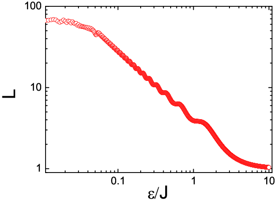
The magnon localization length
| (60) |
is plotted in Figure 9 as a function of the field-gradient.
Appendix B Perturbation Theory
In this section, we present a perturbative solution of the stochastic nonlinear equation including the interaction term for arbitrary field gradients. We expand the normal modes as
| (61) |
and
| (62) |
Keeping only only first-order terms,
We therefore obtain
| zero-order | (63) | |||
| first-order | (64) |
The stationary solution of the zero-order equation is
| (65) |
and that for the first-order one is
| (66) |
The quantity we aim to evaluate is
| (67) |
The first term in the right-hand side of the above equation is simply while the second term is
where correlation
By Isserlis’ (or Wick’s) theorem, we have
where we only keep the non-zero terms. After straightforward substitutions
The perturbative mode temperature (67) is thus given by
| (68) |
In the limit of a very strong Wannier-Zeeman localization, i.e., and ,
| (69) |
which implies absence of mode coupling. The above mode temperature (68) is then modified to
In the limit of a very weak Gilbert damping, only the trivial resonance terms, i.e., and in Eq. (68) survive. We thus have
Higher-order perturbation calculations are straightforward if necessary.
Appendix C Spin Monomer
We implement numerical calculations for a single spin (spin monomer) in contact with a thermal bath corresponding to either an isolated classical atomic moment or a strongly localized normal mode in space. The equation of motion including the magnon interaction is simplified to
| (70) |
where we omitted subscripts. Here source term is the complex noise defined in the main text, with two real-valued Gaussian white noise sources (Wiener process) and .

Figure 10 shows the dynamics of the function We simulate steps with a time step for the time evolution. In numerical calculations, we use parameters and . The Ito interpretation is adopted when integrating the above stochastic differential equation.

The time-average of represents the temperature of the (single) normal mode. Numerical simulations for every are repeated times in order to suppress the statistical error (Figure 10 is just one of them at ). Figure 11 shows the renormalized temperature of the normal mode as a function of the nonlinearity strength . It demonstrates that an increasing nonlinearity increases the temperature of the mode. In the regime of weak nonlinearity the numerical results compare very well with the analytical formula.
Appendix D Spin Dimer
We implement numerical calculations on a spin dimer model contacting with two thermal baths with different temperatures. Under free boundary conditions, the matrix is
| (71) |
In the following, we set The corresponding diagonal matrix
| (72) |
has the eigenvalues
| (73) | ||||
| (74) |
For the equations of motions for the normal modes in the main text become
| (75) | ||||
| (76) |
with
| (77) | ||||
| (78) |
in which source terms and with Gaussian white noises (Wiener process) and .
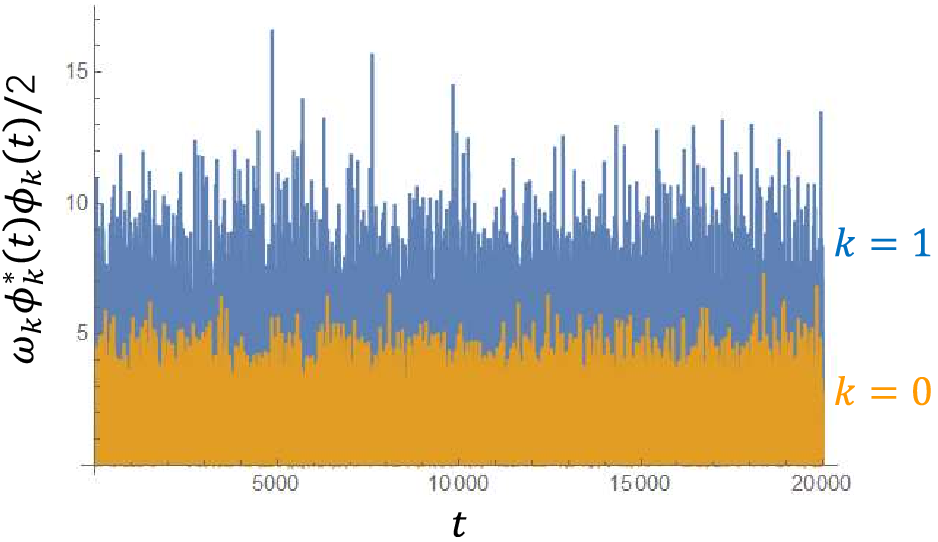
Figure 12 shows the dynamics of function for and We simulate steps with a time step for the time evolution. Parameters used in the numerical calculations are and . Ito interpretation is adopted to integrate the above stochastic differential equations.

The time-average of represents the temperature of the normal mode. Numerical simulations for every are repeated times (Figure 12 is just one of them when ). Figure 13 shows the renormalized temperatures of normal modes as a function of the nonlinearity strength . It demonstrates that an increasing nonlinearity increases the temperature of all modes.
Appendix E Spin Trimer
Numerical calculations of a spin trimer model are presented here. Under free boundary conditions, the matrix is
| (79) |
where we assume Because the analytical form of the eigenvalues and eigenvector of the above matrix is too complicated, we assign a specific number to e.g., The corresponding diagonal matrix then reads
and the eigen values of three normal modes are
| (80) | ||||
| (81) | ||||
| (82) |
In the following numerical calculations, we use parameters The three eigenfrequencies are then and The equations of motions for normal modes become
| (83) | ||||
| (84) | ||||
| (85) |
with
| (86) | ||||
| (87) | ||||
| (88) |
in which source terms and with Gaussian white noises (Wiener process) and .
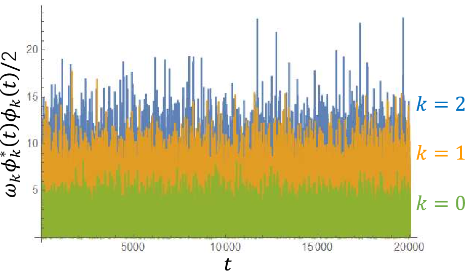
Figure 14 shows the dynamics of function with and We simulate steps with a time step for the time evolution. Ito interpretation is adopted to integrate the above stochastic differential equations.

The time-average of represents the temperature of the normal mode. Numerical simulations for every are repeated times in order to diminish the sample deviation (Figure 14 is one example of them at ). Figure 15 shows the renormalized temperatures of normal modes as a function of the nonlinearity strength . It demonstrates similar red-shift behavior as that in spin dimers.
References
- [1] M. Born and K. Huang, Dynamical Theory of Crystal Lattices (Clarendon Press, Oxford, 1998).
- [2] R.C. Tolman, A General Theory of Energy Partition with Applications to Quantum Theory, Phys. Rev. 11, 261 (1918).
- [3] T. Callen, Thermodynamics 2nd ed. (Wiley, New York, 1985).
- [4] H.H. Rugh, Dynamical Approach to Temperature, Phys. Rev. Lett. 78, 772 (1997).
- [5] T. Speck and U. Seifert, Restoring a fluctuation-dissipation theorem in a nonequilibrium steady state, Europhys. Lett. 74, 391 (2006).
- [6] R. Nandkishore and D.A. Huse, Many-body Localization and Thermalization in Quantum Statistical Mechanics, Annu. Rev. Condens. Matter Phys. 6, 15 (2015).
- [7] G.E.W. Bauer, E. Saitoh, and B.J. van Wees, Spin caloritronics, Nat. Mater. 11, 391 (2012).
- [8] K.R. Narayanan and A.R. Srinivasa, Shannon-entropy-based nonequilibrium “entropic” temperature of a general distribution, Phys. Rev. E 85, 031151 (2012).
- [9] S.-ichi Sasa and Y. Yokokura, Thermodynamic Entropy as a Noether Invariant, Phys. Rev. Lett. 116, 140601 (2016).
- [10] R. Alicki, D. Gelbwaser-Klimovsky, and A. Jenkins, A thermodynamic cycle for the solar cell, arXiv:1606.03819; R. Alicki and D. Gelbwaser-Klimovsky, Non-equilibrium quantum heat machines, New J. Phys. 17, 115012 (2015); P. Calabrese, F.H.L. Essler, and M. Fagotti, Quantum Quench in the Transverse-Field Ising Chain, Phys. Rev. Lett. 106, 227203 (2011).
- [11] K. Miyazaki and K. Seki, Brownian motion of spins revisited, J. Chem. Phys. 108, 7052 (1998).
- [12] W.F. Brown, Jr., Thermal Fluctuations of a Single-Domain Particle, Phys. Rev. 130, 1677 (1963).
- [13] R. Kubo and N. Hashitsume, Brownian Motion of Spins, Prog. Theor. Phys. Suppl. 46, 210 (1970).
- [14] J.L. García-Palacios and F.J. Lázaro, Langevin-dynamics study of the dynamical properties of small magnetic particles, Phys. Rev. B 58, 14937 (1998).
- [15] T.L. Gilbert, A phenomenological theory of damping in ferromagnetic materials, IEEE Trans. Magn. 40, 3443 (2004).
- [16] A. Kawabata, Brownian Motion of a Classical Spin, Prog. Theor. Phys. 48, 2237 (1972).
- [17] A.A. Khajetoorians, B. Baxevanis, C. Hübner, T. Schlenk, S. Krause, T.O. Wehling, S. Lounis, A. Lichtenstein, D. Pfannkuche, J. Wiebe, and R. Wiesendanger, Current-Driven Spin Dynamics of Artificially Constructed Quantum Magnets, Science 339, 55 (2013).
- [18] H.B. Callen and T.A. Welton, Irreversibility and Generalized Noise, Phys. Rev. 83, 34 (1951).
- [19] U. Atxitia, O. Chubykalo-Fesenko, R.W. Chantrell, U. Nowak, and A. Rebei, Ultrafast Spin Dynamics: The Effect of Colored Noise, Phys. Rev. Lett. 102, 057203 (2009).
- [20] A. Rückriegel and P. Kopietz, Rayleigh-Jeans Condensation of Pumped Magnons in Thin-Film Ferromagnets, Phys. Rev. Lett. 115, 157203 (2015).
- [21] V.P. Antropov, V.N. Antonov, L.V. Bekenov, A. Kutepov, and G. Kotliar, Magnetic anisotropic effects and electronic correlations in MnBi ferromagnet, Phys. Rev. B 90, 054404 (2014).
- [22] A. Sukhov, L. Chotorlishvili, A. Ernst, X. Zubizarreta, S. Ostanin, I. Mertig, E.K.U. Gross, and J. Berakdar, Swift thermal steering of domain walls in ferromagnetic MnBi stripes, Sci. Rep. 6, 24411 (2016).
- [23] J.M. Ortiz de Zárate and J.V. Sengers, On the Physical Origin of Long-Ranged Fluctuations in Fuids in Thermal Nonequilibrium States, J. Stat. Phys. 115, 1341 (2004).
- [24] A.-M.S. Tremblay, M. Arai, and E.D. Siggia, Fluctuations about simple nonequilibrium steady states, Phys. Rev. A 23, 1451 (1981).
- [25] L. Bertini, A. De Sole, D. Gabrielli, G. Jona-Lasinio, and C. Landim, Macroscopic fluctuation theory, Rev. Mod. Phys. 87, 593 (2015).
- [26] S. Raghavan, A. Smerzi, S. Fantoni, and S.R. Shenoy, Coherent oscillations between two weakly coupled Bose-Einstein condensates: Josephson effects, oscillations, and macroscopic quantum selft-trapping, Phys. Rev. A 59, 620 (1999).
- [27] S. Geprägs, A. Kehlberger, F.D. Coletta, Z. Qiu, E.-J. Guo, T. Schulz, C. Mix, S. Meyer, A. Kamra, M. Althammer, H. Huebl, G. Jakob, Y. Ohnuma, H. Adachi, J. Barker, S. Maekawa, G.E.W. Bauer, E. Saitoh, R. Gross, S.T.B. Goennenwein, and M. Kläui, Origin of the spin Seebeck effect in compensated ferrimagnets, Nature Commun. 7, 10452 (2016); J. Barker and G.E.W. Bauer, Thermal Spin Dynamics of Yttrium Iron Garnet, Phys. Rev. Lett. 117, 217201 (2016).
- [28] A.V. Savin, G.P. Tsironis, and X. Zotos, Thermal conductivity of a classical one-dimensional spin-phonon system, Phys. Rev. B 75, 214305 (2007).
- [29] B. Jenčič and P. Prelovšek, Spin and thermal conductivity in a classical disordered spin chain, Phys. Rev. B 92, 134305 (2015).
- [30] S.S.-L. Zhang and S. Zhang, Magnon Mediated Electric Current Drag Across a Ferromagnetic Insulator Layer, Phys. Rev. Lett. 109, 096603 (2012).
- [31] D.J. Sanders and D. Walton, Effect of magnon-phonon thermal relaxation on heat transport by magnons, Phys. Rev. B 15, 1489 (1977).
- [32] J. Xiao, G.E.W. Bauer, K. Uchida, E. Saitoh, and S. Maekawa, Theory of magnon-driven spin Seebeck effect, Phys. Rev. B 81, 214418 (2010).
- [33] K.S. Tikhonov, J. Sinova, and A.M. Finkel’stein, Spectral non-uniform temperature and non-local heat transfer in the spin Seebeck effect, Nat. Commun. 4, 1945 (2013).
- [34] U. Ritzmann, D. Hinzke, and U. Nowak, Propagation of thermally induced magnonic spin currents, Phys. Rev. B 89, 024409 (2014).
- [35] K. Uchida, J. Xiao, H. Adachi, J. Ohe, S. Takahashi, J. Ieda, T. Ota, Y. Kajiwara, H. Umezawa, H. Kawai, G.E.W. Bauer, S. Maekawa, and E. Saitoh, Spin Seebeck insulator, Nat. Mater. 9, 894 (2010).
- [36] K. Uchida, H. Adachi, T. Ota, H. Nakayama, S. Maekawa, and E. Saitoh, Observation of longitudinal spin-Seebeck effect in magnetic insulators, Appl. Phys. Lett. 97, 172505 (2010).
- [37] S.Y. Huang, X. Fan, D. Qu, Y.P. Chen, W.G. Wang, J. Wu, T.Y. Chen, J.Q. Xiao, and C.L. Chien, Transport Magnetic Proximity Effects in Platinum, Phys. Rev. Lett. 109, 107204 (2012).
- [38] D. Qu, S.Y. Huang, J. Hu, R. Wu, and C.L. Chien, Intrinsic Spin Seebeck Effect in Au/YIG, Phys. Rev. Lett. 110, 067206 (2013).
- [39] M. Weiler, M. Althammer, F.D. Czeschka, H. Huebl, M.S. Wagner, M. Opel, I.-M. Imort, G. Reiss, A. Thomas, R. Gross, and S.T.B. Goennenwein, Local Charge and Spin Currents in Magnetothermal Landscapes, Phys. Rev. Lett. 108, 106602 (2012).
- [40] K. Uchida, T Kikkawa, A Miura, J Shiomi, and E. Saitoh, Quantitative Temperature Dependence of Longitudinal Spin Seebeck Effect at High Temperatures, Phys. Rev. X 4, 041023 (2014).
- [41] A. Kehlberger, U. Ritzmann, D. Hinzke, E.-J. Guo, J. Cramer, G. Jakob, M.C. Onbasli, D.H. Kim, C.A. Ross, M.B. Jungfleisch, B. Hillebrands, U. Nowak, and M. Kläui, Length Scale of the Spin Seebeck Effect, Phys. Rev. Lett. 115, 096602 (2015).
- [42] C.M. Jaworski, J. Yang, S. Mack, D.D. Awschalom, J.P. Heremans, and R.C. Myers, Observation of the spin-Seebeck effect in a ferromagnetic semiconductor, Nat. Mater. 9, 898 (2010).
- [43] C.M. Jaworski, R.C. Myers, E. Johnston-Halperin, and J.P. Heremans, Giant spin Seebeck effect in a non-magnetic material, Nature (London) 487, 210 (2012).
- [44] A.D. Avery, M.R. Pufall, and B.L. Zink, Observation of the Planar Nernst Effect in Permalloy and Nickel Thin Films with In-Plane Thermal Gradients, Phys. Rev. Lett. 109, 196602 (2012).
- [45] M. Schmid, S. Srichandan, D. Meier, T. Kusche, J.-M. Schmalhorst, M. Vogel, G. Reiss, C. Strunk, and C.H. Back, Transverse Spin Seebeck Effect versus Anomalous and Planar Nernst Effects in Permalloy Thin Films, Phys. Rev. Lett. 111, 187201 (2013).
- [46] D. Meier, D. Reinhardt, M. van Straaten, C. Klewe, M. Althammer, M. Schreier, S.T.B. Goennenwein, A. Gupta, M. Schmid, C.H. Back, J.-M. Schmalhorst, T. Kuschel, and G. Reiss, Longitudinal spin Seebeck effect contribution in transverse spin Seebeck effect experiments in Pt/YIG and Pt/NFO, Nat. Commun. 6, 8211 (2015).
- [47] J. Shan, L.J. Cornelissen, N. Vlietstra, J.B. Youssef, T. Kuschel, R.A. Duine, and B.J. van Wees, Influence of yttrium iron garnet thickness and heater opacity on the nonlocal transport of electrically and thermally excited magnons, Phys. Rev. B 94, 174437 (2016).
- [48] H. Jiao and G.E.W. Bauer, Spin Backflow and ac Voltage Generation by Spin Pumping and the Inverse Spin Hall Effect, Phys. Rev. Lett. 110, 217602 (2013).
- [49] K. Chen and S. Zhang, Spin Pumping in the Presence of Spin-Orbit Coupling, Phys. Rev. Lett. 114, 126602 (2015).
- [50] D. Emin and C.F. Hart, Existence of Wannier-Stark localization, Phys. Rev. B 36, 7353 (1987).
- [51] F.H. de Leeuw, Wall velocity in garnet films at high drive fields, IEEE Trans. Magn. 13, 1172 (1977).
- [52] C. Tsang, C. Bonhote, Q. Dai, H. Do, B. Knigge, Y. Ikeda, Q. Le, B. Lengsfield, J. Lille, J. Li, S. MacDonald, A. Moser, V. Nayak, R. Payne, N. Robertson, M. Schabes, N. Smith, K. Takano, P. van der Heijden, W. Weresin, M. Williams, and M. Xiao, Head challenges for perpendicular recording at high areal density, IEEE Trans. Magn. 42, 145 (2006).
- [53] J.M.D. Coey, New permanent magnets; mangnese compounds, J. Phys.: Condens. Matter 26, 064211 (2014).
- [54] K.S. Novoselov, A.K. Geim, S.V. Dubonos, E.W. Hill, and I.V. Grigorieva, Subatomic movements of a domain wall in the Peierls potential, Nature (London) 426, 812 (2003).
- [55] V. Cherepanov, I. Kolokolov, and V. L’vov, The saga of YIG: spectra, thermodynamics, interaction and relaxation of magnons in a complex magnet, Phys. Rep. 229, 81 (1993).
- [56] A. Kreisel, F. Saulo, L. Bartosch, and P. Kopietz, Microscopic spin-wave theory for yttrium-iron garnet films, Eur. Phys. J. B 71, 59 (2009).
- [57] F. Rossi, Bloch oscillations and Wannier-Stark localization in semiconductor superlattices, in: Theory of Transport Properties of Semiconductor Nanostructures, edited by E. Schöll, (Spinger, Boston, 1998), pp. 283–320.
- [58] A.M. Kosevich, B.A. Ivanov, and A.S. Kovalev, Magnetic Solitons, Phys. Rep. 194, 117 (1990).
- [59] A. Slavin and V. Tiberkevich, Nonlinear Auto-Oscillator Theory of Microwave Generation by Spin-Polarized Current, IEEE Trans. Magn. 45, 1875 (2009).
- [60] S. Borlenghi, S. Iubini, S. Lepri, J. Chico, L. Bergqvist, A. Delin, and J. Fransson, Energy and magnetization transport in nonequilibrium macrospin systems, Phys. Rev. E 92, 012116 (2015).