跳到论文正文
W Papers独立论文阅读器 arXiv:1604.08086 论文正文 计算阅读时间 · 0%
引用这篇论文根据当前论文元数据生成,正式投稿前建议核对。


License: arXiv.org perpetual non-exclusive license
arXiv:1604.08086v2 [eess.SY] 23 Jun 2016

Balanced model order reduction for systems depending on a parameter1

Carles Batlle Affiliation: Carles Batlle is with Departament de Matemàtiques, EPSEVG and IOC, Universitat Politècnica de Catalunya — BarcelonaTech, Vilanova i la Geltrú, Spain: carles.batlle@upc.edu, ORCID:0000-0002-6088-6187    Néstor Roqueiro Affiliation:  Néstor Roqueiro is with Departamento de Automação e Sistemas, Universidade Federal de Santa Catarina, Florianópolis, Brasil: nestor.roqueiro@ufsc.br Affiliation:  This paper is a preprint of a paper submitted to IET Control Theory and Applications, and is subject to Institution of Engineering and Technology Copyright. If accepted, the copy of record will be available at IET Digital Library.
Abstract

We provide an analytical framework for balanced realization model order reduction of linear control systems which depend on an unknown parameter. Besides recovering known results for the first order corrections, we obtain explicit novel expressions for the form of second order corrections for singular values and singular vectors. The final result of our procedure is an order reduced model which incorporates the uncertain parameter. We apply our algorithm to the model order reduction of a linear system of masses and springs with parameter dependent coefficients.

I INTRODUCTION

Order reduced models [14] are useful to simulate very large models using less computational resources, allowing, for instance, the exploration of parameter regions. The lower order model should have some desirable properties, such as being easily computable, preserving some of the structural properties of the full model and, more importantly, yielding an error with respect to the original model that can be bounded in terms of the complexity of the approximating model. In particular, for linear time-invariant MIMO systems, model order reduction (MOR) based on the truncation of balanced realizations preserves the stability, controllability and observability of the full model, and furthermore provides bounds for the norm of the error system [1].

The computation of a balanced realization for a linear system relies on numerical linear algebra algorithms, and does not allow for the presence of symbolic parameters in the model. Hence, if a system contains an uncertain parameter, appearing, for instance, due to a physical coefficient which is only known to belong to a given interval, or due to the specification of a working point in a nonlinear system, the balancing procedure must be carried out for each numerical value of the parameter. This results in a set of reduced order models, which are difficult to work with if they are to be used to design a controller and, in any case, the explicit dependence on the original parameter is lost in the reduced system.

In this paper we work out an algorithm to obtain a reduced order model which incorporates the original, symbolical parameter through a polynomial of arbitrary degree. To this end, we solve each step of the balanced realization procedure in powers of the symbolical parameter, although for the last step, which involves a singular value decomposition (SVD), we only provide explicit expressions up to second order corrections. Up to our knowledge, the second order correction to the singular subspaces that we obtain has not been reported in the literature, and it may be useful in other applications of SVD.

The paper is organized as follows. Section II reviews the steps of the computation of the balanced realization for linear systems, and how a reduced order model can be constructed from it. Section III develops a power series expansion for each of the above steps. We give explicit algorithms for each step, except for the singular value decomposition, which we develop only to second order. Section IV applies the procedure to a system of masses and springs with parameter dependent coefficients, and, finally, we discuss our results and point to possible improvements in Section V.

II REVIEW OF THE BALANCED REALIZATION PROCEDURE

Consider the nonlinear control system

x˙\displaystyle\dot{x} =\displaystyle= f⁡(x)+g⁡(x)​u,\displaystyle f(x)+g(x)u, (1)
y\displaystyle y =\displaystyle= h⁡(x),\displaystyle h(x), (2)

with x∈ℝNx\in\mathbb{R}^{N}, u∈ℝMu\in\mathbb{R}^{M}, y∈ℝPy\in\mathbb{R}^{P} and f⁡(0)=0f(0)=0.

The controllability function Lc​(x)L_{c}(x) is the solution of the optimal control problem

Lc​(x)=infu∈L2​((−∞,0),ℝM)12​∫−∞0‖u⁡(t)‖2​d​tL_{c}(x)=\inf_{u\in L^{2}((-\infty,0),\mathbb{R}^{M})}\frac{1}{2}\int_{-\infty}^{0}||u(t)||^{2}\text{d}t (3)

subject to the boundary conditions x⁡(−∞)=0x(-\infty)=0, x⁡(0)=xx(0)=x and the system (1). Roughly speaking, Lc​(x)L_{c}(x) measures the minimum 2-norm of the input signal necessary to bring the system to the state xx from the origin.

As shown in [13], LcL_{c} obeys the Hamilton-Jacobi-Bellman PDE

∂xLc​f+12​∂xLc​g​gT​∂xTLc=0,Lc​(0)=0,\partial_{x}L_{c}f+\frac{1}{2}\partial_{x}L_{c}gg^{T}\partial_{x}^{T}L_{c}=0,\quad L_{c}(0)=0, (4)

in a domain Uc⊂ℝNU_{c}\subset\mathbb{R}^{N} which contains the origin and where the vector field −(f+g​gT​∂xTLc)-(f+gg^{T}\partial_{x}^{T}L_{c}) is asymptotically stable.

The observability function Lo​(x)L_{o}(x) is the 2-norm of the output signal obtained when the system is relaxed from the state xx

Lo​(x)=12​∫0∞‖y⁡(t)‖2​d​t=12​∫0∞‖h⁡(x⁡(t))‖2​d​t,L_{o}(x)=\frac{1}{2}\int_{0}^{\infty}||y(t)||^{2}\text{d}t=\frac{1}{2}\int_{0}^{\infty}||h(x(t))||^{2}\text{d}t, (5)

with x⁡(0)=xx(0)=x and subjected to (1) with u=0u=0, that is, x˙=f⁡(x)\dot{x}=f(x). It obeys the Lyapunov PDE

∂xLo​f+12​hT​h=0,Lo​(0)=0,\partial_{x}L_{o}f+\frac{1}{2}h^{T}h=0,\quad L_{o}(0)=0, (6)

in a domain Uo⊂ℝNU_{o}\subset\mathbb{R}^{N} around the origin where f⁡(x)f(x) is asymptotically stable.

For linear control systems,

x˙\displaystyle\dot{x} =\displaystyle= A​x+B​u,\displaystyle Ax+Bu, (7)
y\displaystyle y =\displaystyle= C​x,\displaystyle Cx, (8)

assumed to be observable, controllable and Hurwitz, both Lc​(x)L_{c}(x) and Lo​(x)L_{o}(x) are quadratic functions

Lc​(x)\displaystyle L_{c}(x) =\displaystyle= 12​xT​Wc−1​x,\displaystyle\frac{1}{2}x^{T}W_{c}^{-1}x, (9)
L0​(x)\displaystyle L_{0}(x) =\displaystyle= 12​xT​Wo​x,\displaystyle\frac{1}{2}x^{T}W_{o}x, (10)

where Wc>0W_{c}>0 and Wo>0W_{o}>0, the controllability and observability Gramians, are the solutions to the matrix Lyapunov equations

A​Wc+Wc​AT+B​BT\displaystyle AW_{c}+W_{c}A^{T}+BB^{T} =\displaystyle= 0,\displaystyle 0, (11)
AT​Wo+Wo​A+CT​C\displaystyle A^{T}W_{o}+W_{o}A+C^{T}C =\displaystyle= 0.\displaystyle 0. (12)

As shown by Moore ([10]; see also [7], [17] and [16]), the matrix WcW_{c} provides information about the states that are easy to control (in the sense that signals uu of small norm can be used to reach them), while WoW_{o} allows to find the states that are easily observable (in the sense that they produce outputs of large norm). From the point of view of the input-output map given by (7) (8), one would like to select the states that score well on both counts, and this leads to the concept of balanced realization, for which Wc=WoW_{c}=W_{o}.

The balanced realization is obtained by means of a linear transformation x=T​zx=Tz, with TT computed as follows:

  1. 1.

    Solve the Lyapunov equations

    A​Wc+Wc​AT+B​BT\displaystyle AW_{c}+W_{c}A^{T}+BB^{T} =\displaystyle= 0,\displaystyle 0, (13)
    AT​Wo+Wo​A+CT​C\displaystyle A^{T}W_{o}+W_{o}A+C^{T}C =\displaystyle= 0,\displaystyle 0, (14)

    with solutions Wc>0W_{c}>0, Wo>0W_{o}>0.

  2. 2.

    Perform Cholesky factorizations of the Gramians:

    Wc=X​XT,Wo=Y​YT.W_{c}=XX^{T},\quad W_{o}=YY^{T}. (15)

    Notice that X>0X>0 and Y>0Y>0.

  3. 3.

    Compute the SVD of YT​XY^{T}X:

    YT​X=U​Σ​VT,Y^{T}X=U\Sigma V^{T}, (16)

    with UU and VV orthogonal and

    Σ=diag​(σ1,σ2,…,σN),with​σ1>σ2>⋯>σN>0.\Sigma=\text{diag}(\sigma_{1},\sigma_{2},\ldots,\sigma_{N}),\quad\text{with}\ \sigma_{1}>\sigma_{2}>\cdots>\sigma_{N}>0. (17)

    The σi\sigma_{i} are the Hankel singular values, and their squares τi=σi2\tau_{i}=\sigma_{i}^{2} are often referred to as the squared singular values of the control system.

  4. 4.

    The balancing transformation is given then by

    T=XVΣ−1/2,withT−1=Σ−1/2UTYT.T=XV\Sigma^{-1/2},\quad\text{with}\ T^{-1}=\Sigma^{-1/2}U^{T}Y^{T}. (18)
  5. 5.

    The balanced realization is given by the linear system

    A~=T−1​A​T,B~=T−1​B,C~=C​T,\tilde{A}=T^{-1}AT,\quad\tilde{B}=T^{-1}B,\quad\tilde{C}=CT, (19)

    and in the new coordinates

    W~c\displaystyle\tilde{W}_{c} =\displaystyle= T−1​Wc​T−T=Σ,\displaystyle T^{-1}W_{c}T^{-T}=\Sigma, (20)
    W~o\displaystyle\tilde{W}_{o} =\displaystyle= TT​Wo​T=Σ.\displaystyle T^{T}W_{o}T=\Sigma. (21)

Notice that, in the balanced realization,

L~c​(z)\displaystyle\tilde{L}_{c}(z) =\displaystyle= 12​∑i=1Nzi2σi=12​zT​Σ−1​z,\displaystyle\frac{1}{2}\sum_{i=1}^{N}\frac{z_{i}^{2}}{\sigma_{i}}=\frac{1}{2}z^{T}\Sigma^{-1}z, (22)
L~o​(z)\displaystyle\tilde{L}_{o}(z) =\displaystyle= 12​∑i=1Nσi​zi2=12​zT​Σ​z,\displaystyle\frac{1}{2}\sum_{i=1}^{N}\sigma_{i}z_{i}^{2}=\frac{1}{2}z^{T}\Sigma z, (23)

so that the state with only nonzero coordinate ziz_{i} is both easier to control and easier to observe than the state corresponding to zi+1z_{i+1}, for i=1,2,…,N−1i=1,2,\ldots,N-1. If, for a given rr, 1≤r<N1\leq r<N, one has σr≫σr+1\sigma_{r}\gg\sigma_{r+1}, it may be sensible, from the point of view of the map between uu and yy, to keep just the states corresponding to the coordinates z1,z2,…,zrz_{1},z_{2},\ldots,z_{r}, and this is what is known as balanced realization model order reduction.

ℋ∞\mathcal{H}_{\infty}-norm lower and upper error bounds of the balanced truncation method are given by

σr+1≤‖G⁡(s)−Gr​(s)‖ℋ∞≤2​∑i=r+1nσi,\sigma_{r+1}\leq\|G(s)-G_{r}(s)\|_{\mathcal{H}_{\infty}}\leq 2\sum_{i=r+1}^{n}\sigma_{i}, (24)

where σi,i=1,…,n\sigma_{i},i=1,\dots,n, are the Hankel singular values of the system [6][5] (see [1] for a thorough review, and references therein). From these inequalities it follows that, in order to get the smallest error for the truncated system, one should disregard the states associated with the smallest Hankel singular values (but see [9][11] for a tighter lower bound that sometimes might yield a better approximation).

If we denote by A~r\tilde{A}_{r} the upper-left square block of A~\tilde{A} formed by the first rr rows and columns, and by B~r\tilde{B}_{r} and C~r\tilde{C}_{r} the matrices obtained from the first rr rows or columns of B~\tilde{B} or C~\tilde{C}, respectively, the reduced system of order rr obtained by balanced truncation is given by

Z˙r\displaystyle\dot{Z}_{r} =\displaystyle= A~r​Zr+B~r​u,\displaystyle\tilde{A}_{r}Z_{r}+\tilde{B}_{r}u, (25)
y\displaystyle y =\displaystyle= C~r​Zr,\displaystyle\tilde{C}_{r}Z_{r}, (26)

with Zr=(z1,…,zr)Z_{r}=(z_{1},\ldots,z_{r}).

One of the problems of the above procedure is that it does not allow for the presence of symbolic parameters in the problem, since the solution of the matrix equations involved relies on numerical methods. In this paper we address this issue, assuming that the linear system is given by matrices A⁡(m)A(m), B⁡(m)B(m) and C⁡(m)C(m) which depend analytically on the parameter mm. This may represent an uncertain physical coefficient (this is the case of the example in Section IV), or it may appear by considering an unspecified working point in the linearization of a nonlinear system. Indeed, assume that (1) has a curve of fixed points x=x⁡(ξ)x=x(\xi), u=u⁡(x⁡(ξ))u=u(x(\xi)), with ξ∈ℝ\xi\in\mathbb{R} the parameter of the curve, i.e. such that

f⁡(x⁡(ξ))+g⁡(x⁡(ξ))​u​(x⁡(ξ))=0,for all ξ in an open set.f(x(\xi))+g(x(\xi))u(x(\xi))=0,\quad\text{for all $\xi$ in an open set.}

Consider now a given value ξ0\xi_{0} of ξ\xi, and let z=x−x0z=x-x_{0}, with x0=x⁡(ξ0)x_{0}=x(\xi_{0}), and v=u−u⁡(x⁡(ξ0))v=u-u(x(\xi_{0})). One obtains immediately that the corresponding linearization of (1) is given by

z˙=F⁡(ξ0)​z+G⁡(ξ0)​v,\dot{z}=F(\xi_{0})z+G(\xi_{0})v, (27)

where FF, GG are, respectively, N×NN\times N and N×MN\times M matrices with elements

Fi​j​(ξ0)\displaystyle F_{ij}(\xi_{0}) =\displaystyle= ∂jfi​(x0)+∑k=1M∂jgi​k​(x0)​u0​k​(x0),i,j=1,…​N,\displaystyle\partial_{j}f_{i}(x_{0})+\sum_{k=1}^{M}\partial_{j}g_{ik}(x_{0})u_{0k}(x_{0}),\quad i,j=1,\ldots N, (28)
Gi​j​(ξ0)\displaystyle G_{ij}(\xi_{0}) =\displaystyle= gi​j​(x0),i=1,…​N,j=1,…​M.\displaystyle g_{ij}(x_{0}),\quad i=1,\ldots N,\ j=1,\ldots M. (29)

Furthermore, writing w=y−h⁡(x0)w=y-h(x_{0}), the linearization of (2) yields

w=H(ξ0)z,Hi​j(ξ0)=∂jhi(x0),i=1,…,P,j=1,…,N.w=H(\xi_{0})z,\quad H_{ij}(\xi_{0})=\partial_{j}h_{i}(x_{0}),\ i=1,\ldots,P,\ j=1,\ldots,N. (30)

Let ξ^0\hat{\xi}_{0} be an specific, i.e. numeric, value of ξ0\xi_{0} that we take as a reference working point, and let m=ξ0−ξ^0m=\xi_{0}-\hat{\xi}_{0}, and define

A⁡(m)=F⁡(ξ^0+m),B⁡(m)=G⁡(ξ^0+m),C⁡(m)=H⁡(ξ^0+m).A(m)=F(\hat{\xi}_{0}+m),\ B(m)=G(\hat{\xi}_{0}+m),\ C(m)=H(\hat{\xi}_{0}+m).

Our goal is to develop a power series expansion in mm of the balanced model order reduction algorithm for the linear input/output system given by A⁡(m)A(m), B⁡(m)B(m), C⁡(m)C(m). This will facilitate the analysis of how much the important degrees of freedom vary when mm is changed and, more importantly, will yield a reduced order model, suitable for control design, which incorporates the dependence on mm in an explicit way. A survey of other approaches to this problem is presented in [4].

III POWER SERIES EXPANSION FOR THE BALANCED REALIZATION

Following the previous discussion, consider the control system

x˙\displaystyle\dot{x} =\displaystyle= A⁡(m)​x+B⁡(m)​u,\displaystyle A(m)x+B(m)u, (31)
y\displaystyle y =\displaystyle= C⁡(m)​x,\displaystyle C(m)x, (32)

with mm a symbolic parameter. The controllability Gramian will depend also on mm, and will be given by the solution Wc​(m)W^{c}(m) to the Lyapunov equation

A⁡(m)​Wc​(m)+Wc​(m)​AT​(m)+B⁡(m)​BT​(m)=0.A(m)W^{c}(m)+W^{c}(m)A^{T}(m)+B(m)B^{T}(m)=0. (33)

Assume that A⁡(m)A(m), B⁡(m)B(m) and C⁡(m)C(m) are analytic in mm,

A⁡(m)\displaystyle A(m) =\displaystyle= ∑k=0∞Ak​mk,\displaystyle\sum_{k=0}^{\infty}A_{k}m^{k}, (34)
B⁡(m)\displaystyle B(m) =\displaystyle= ∑k=0∞Bk​mk,\displaystyle\sum_{k=0}^{\infty}B_{k}m^{k}, (35)
C⁡(m)\displaystyle C(m) =\displaystyle= ∑k=0∞Ck​mk,\displaystyle\sum_{k=0}^{\infty}C_{k}m^{k}, (36)

and let us look for likewise solutions of the form

Wc​(m)=∑k=0∞Wkc​mk.W^{c}(m)=\sum_{k=0}^{\infty}W^{c}_{k}m^{k}. (37)

Using the formal identities

∑k=0∞ak​tk​∑j=0∞bj​tj=∑r=0∞(∑s=0rar−s​bs)​tr=∑r=0∞(∑s=0ras​br−s)​tr,\sum_{k=0}^{\infty}a_{k}t^{k}\ \sum_{j=0}^{\infty}b_{j}t^{j}=\sum_{r=0}^{\infty}\left(\sum_{s=0}^{r}a_{r-s}b_{s}\right)t^{r}=\sum_{r=0}^{\infty}\left(\sum_{s=0}^{r}a_{s}b_{r-s}\right)t^{r}, (38)

and substituting the above expansions into (33) one immediately obtains

∑s=0r(Ar−s​Wsc+Wsc​Ar−sT+Br−s​BsT)=0,for r=0,1,2,….\sum_{s=0}^{r}\left(A_{r-s}W^{c}_{s}+W^{c}_{s}A_{r-s}^{T}+B_{r-s}B_{s}^{T}\right)=0,\quad\text{for $r=0,1,2,\ldots$}. (39)

These are equivalent to the set of Lyapunov equations

A0​W0c+W0c​A0T+B0​B0T\displaystyle A_{0}W^{c}_{0}+W^{c}_{0}A_{0}^{T}+B_{0}B_{0}^{T} =\displaystyle= 0,\displaystyle 0, (40)
A0​Wrc+Wrc​A0T+Pr\displaystyle A_{0}W^{c}_{r}+W^{c}_{r}A_{0}^{T}+P_{r} =\displaystyle= 0,r=1,2,…,\displaystyle 0,\ r=1,2,\ldots, (41)

with

Pr=B0BrT+∑s=0r−1(Ar−sWsc+WscAr−sT+Br−sBsT),r=1,2,…P_{r}=B_{0}B_{r}^{T}+\sum_{s=0}^{r-1}\left(A_{r-s}W^{c}_{s}+W^{c}_{s}A_{r-s}^{T}+B_{r-s}B_{s}^{T}\right),\quad r=1,2,\ldots (42)

These equations can be solved recursively to the desired order, starting with the zeroth order Lyapunov equation (40). Observe that the internal dynamics is always given by A0A_{0}, and that it is only the effective control term PrP_{r} the one that changes with the order.

Similarly, the observability Gramian Wo​(m)W^{o}(m) satisfies

AT​(m)​Wo​(m)+Wo​(m)​A​(m)+CT​(m)​C​(m)=0,A^{T}(m)W^{o}(m)+W^{o}(m)A(m)+C^{T}(m)C(m)=0, (43)

and its power series solution

Wo​(m)=∑k=0∞Wko​mk,W^{o}(m)=\sum_{k=0}^{\infty}W^{o}_{k}m^{k}, (44)

can be obtained recursively from

A0T​W0o+W0o​A0+C0T​C0\displaystyle A^{T}_{0}W^{o}_{0}+W^{o}_{0}A_{0}+C^{T}_{0}C_{0} =\displaystyle= 0,\displaystyle 0, (45)
A0T​Wro+Wro​A0+Qr\displaystyle A^{T}_{0}W^{o}_{r}+W^{o}_{r}A_{0}+Q_{r} =\displaystyle= 0,r=1,2,…,\displaystyle 0,\ r=1,2,\ldots, (46)

with

Qr=C0TCr+∑s=0r−1(Ar−sTWso+WsoAr−s+Cr−sTCs),r=1,2,…Q_{r}=C^{T}_{0}C_{r}+\sum_{s=0}^{r-1}\left(A^{T}_{r-s}W^{o}_{s}+W^{o}_{s}A_{r-s}+C^{T}_{r-s}C_{s}\right),\quad r=1,2,\ldots (47)

After computing Wc​(m)W^{c}(m) and Wo​(m)W^{o}(m) at the desired order, the next step in the balancing transformation procedure is to compute their “square roots”, X⁡(m)X(m) and Y⁡(m)Y(m), such that

Wc​(m)\displaystyle W^{c}(m) =\displaystyle= X⁡(m)​XT​(m),\displaystyle X(m)X^{T}(m), (48)
Wo​(m)\displaystyle W^{o}(m) =\displaystyle= Y⁡(m)​YT​(m).\displaystyle Y(m)Y^{T}(m). (49)

If

X⁡(m)=∑k=0∞Xk​mk,X(m)=\sum_{k=0}^{\infty}X_{k}m^{k}, (50)

one gets

Wkc=∑s=0kXk−s​XsT,W^{c}_{k}=\sum_{s=0}^{k}X_{k-s}X^{T}_{s}, (51)

which, again, are solved recursively as

X0​X0T\displaystyle X_{0}X_{0}^{T} =\displaystyle= W0c,\displaystyle W_{0}^{c}, (52)
Xk​X0T+X0​XkT\displaystyle X_{k}X_{0}^{T}+X_{0}X_{k}^{T} =\displaystyle= Wkc−∑s=1k−1Xk−s​XsT.\displaystyle W_{k}^{c}-\sum_{s=1}^{k-1}X_{k-s}X_{s}^{T}. (53)

Similarly, for

Y⁡(m)=∑k=0∞Yk​mk,Y(m)=\sum_{k=0}^{\infty}Y_{k}m^{k}, (54)

one arrives at

Y0​Y0T\displaystyle Y_{0}Y_{0}^{T} =\displaystyle= W0o,\displaystyle W_{0}^{o}, (55)
Yk​Y0T+Y0​YkT\displaystyle Y_{k}Y_{0}^{T}+Y_{0}Y_{k}^{T} =\displaystyle= Wko−∑s=1k−1Yk−s​YsT.\displaystyle W_{k}^{o}-\sum_{s=1}^{k-1}Y_{k-s}Y_{s}^{T}. (56)

Equations (52) and (55) are standard Cholesky equations, but (53) and (56) are not Lyapunov (or Sylvester) equations for XkX_{k} or YkY_{k} because of the presence of XkTX_{k}^{T} and YkTY_{k}^{T}, respectively.

Equations of the form A​X+XT​B=CAX+X^{T}B=C for XX have been studied in [18], where the problem is reduced to a sequence of low-order linear systems for the entries of XX. However, the conditions for the uniqueness of the solution stated in [18] are not satisfied by equations of the form of (53). Indeed, in order to solve (53) one has to consider det(X0+λ​(X0T)T)=(1+λ)N​detX0\det(X_{0}+\lambda(X_{0}^{T})^{T})=(1+\lambda)^{N}\det X_{0}, which vanishes for λ=−1\lambda=-1 and thus violates condition (2) of Theorem 3 in [18]. Notice, however, that the right-hand side of (53) is a symmetric matrix. If one splits XkX_{k} into symmetric, SkS_{k}, and skew-symmetric, TkT_{k}, parts, one gets, after some calculations, that they obey

Sk​X0T+X0​Sk\displaystyle S_{k}X_{0}^{T}+X_{0}S_{k} =\displaystyle= Wkc−∑s=1k−1Xk−s​XsT,\displaystyle W_{k}^{c}-\sum_{s=1}^{k-1}X_{k-s}X_{s}^{T}, (57)
Tk​X0T+X0​Tk\displaystyle T_{k}X_{0}^{T}+X_{0}T_{k} =\displaystyle= 0.\displaystyle 0. (58)

Equations (57) and (58) are Lyapunov equations, and in fact the generic solution to (58) is Tk=0T_{k}=0. Hence, we have that the solution to (53) is given by

Xk=Sk,X_{k}=S_{k}, (59)

with SkS_{k} the solution to the Lyapunov equation (57), and an analogous reasoning applies to the solution of (56).

The last nontrivial step in the balancing algorithm is the singular value decomposition (SVD) of the product YT​(m)​X​(m)Y^{T}(m)X(m),

YT​(m)​X​(m)=U⁡(m)​Σ​(m)​VT​(m),Y^{T}(m)X(m)=U(m)\Sigma(m)V^{T}(m), (60)

where

Σ⁡(m)=diag​(σ1​(m)≥σ2​(m)≥…≥σn​(m)>0),\Sigma(m)=\text{diag}(\sigma_{1}(m)\geq\sigma_{2}(m)\geq\ldots\geq\sigma_{n}(m)>0), (61)

and U⁡(m)U(m) and V⁡(m)V(m) are N×NN\times N orthogonal matrices, depending also on the parameter mm.

Let us denote by RkR_{k} the coefficients of the power series of YT​(m)​X​(m)Y^{T}(m)X(m),

YT​(m)​X​(m)=∑k=0∞Rk​mk,Y^{T}(m)X(m)=\sum_{k=0}^{\infty}R_{k}m^{k}, (62)

with

Rk=∑s=0kYk−sT​Xs=∑s=0kYsT​Xk−s.R_{k}=\sum_{s=0}^{k}Y_{k-s}^{T}X_{s}=\sum_{s=0}^{k}Y_{s}^{T}X_{k-s}. (63)

Let also

U⁡(m)\displaystyle U(m) =\displaystyle= ∑k=0∞Uk​mk,\displaystyle\sum_{k=0}^{\infty}U_{k}m^{k}, (64)
V⁡(m)\displaystyle V(m) =\displaystyle= ∑k=0∞Vk​mk,\displaystyle\sum_{k=0}^{\infty}V_{k}m^{k}, (65)
Σ⁡(m)\displaystyle\Sigma(m) =\displaystyle= ∑k=0∞Σk​mk.\displaystyle\sum_{k=0}^{\infty}\Sigma_{k}m^{k}. (66)

Notice that the coefficients of the power series for V−1​(m)V^{-1}(m),

V−1​(m)=∑k=0∞V^k​mk,V^{-1}(m)=\sum_{k=0}^{\infty}\hat{V}_{k}m^{k}, (67)

can be computed recursively from those of V⁡(m)V(m) as

V^0\displaystyle\hat{V}_{0} =\displaystyle= V0−1,\displaystyle V_{0}^{-1}, (68)
V^k\displaystyle\hat{V}_{k} =\displaystyle= −V0−1∑s=1kVsV^k−s,k=1,2,…\displaystyle-V_{0}^{-1}\sum_{s=1}^{k}V_{s}\hat{V}_{k-s},\quad k=1,2,\ldots (69)

provided that V0V_{0} is invertible, which is the case since we are assuming that V⁡(m)V(m) is orthogonal for all mm, and in particular for m=0m=0. For k=1k=1 and k=2k=2 one has, explicitly,

V^1\displaystyle\hat{V}_{1} =\displaystyle= −V0−1​V1​V0−1,\displaystyle-V_{0}^{-1}V_{1}V_{0}^{-1}, (70)
V^2\displaystyle\hat{V}_{2} =\displaystyle= −V0−1​V2​V0−1+V0−1​V1​V0−1​V1​V0−1.\displaystyle-V_{0}^{-1}V_{2}V_{0}^{-1}+V_{0}^{-1}V_{1}V_{0}^{-1}V_{1}V_{0}^{-1}. (71)

However, we will not need to compute the coefficients of V−1​(m)V^{-1}(m), as we will presently see. From now on we will consider approximations only up to second order. As it will be clear from our presentation, obtaining higher order approximations is immediate but involves expressions that become quite cumbersome. We will write

R⁡(m)\displaystyle R(m) =\displaystyle= R0+m​R1+m2​R2,\displaystyle R_{0}+mR_{1}+m^{2}R_{2}, (72)
U⁡(m)\displaystyle U(m) =\displaystyle= U0+m​U1+m2​U2,\displaystyle U_{0}+mU_{1}+m^{2}U_{2}, (73)
V⁡(m)\displaystyle V(m) =\displaystyle= V0+m​V1+m2​V2,\displaystyle V_{0}+mV_{1}+m^{2}V_{2}, (74)
Σ⁡(m)\displaystyle\Sigma(m) =\displaystyle= Σ0+m​Σ1+m2​Σ2,\displaystyle\Sigma_{0}+m\Sigma_{1}+m^{2}\Sigma_{2}, (75)

with the understanding that any higher order contribution is neglected. From R=U​Σ​VTR=U\Sigma V^{T} one gets the identities

R​V\displaystyle RV =\displaystyle= U​Σ,\displaystyle U\Sigma, (76)
RT​U\displaystyle R^{T}U =\displaystyle= V​Σ,\displaystyle V\Sigma, (77)

which in turn inply

RT​R​V\displaystyle R^{T}RV =\displaystyle= V​Σ2,\displaystyle V\Sigma^{2}, (78)
R​RT​U\displaystyle RR^{T}U =\displaystyle= U​Σ2.\displaystyle U\Sigma^{2}. (79)

If we denote by uj(k)u_{j}^{(k)} the jjth column vector of UkU_{k}, and by vj(k)v_{j}^{(k)} the one of VkV_{k}, equations (76) and (77) imply

(R0+m​R1+m2​R2)​(vj(0)+m​vj(1)+m2​vj(2))\displaystyle(R_{0}+mR_{1}+m^{2}R_{2})(v_{j}^{(0)}+mv_{j}^{(1)}+m^{2}v_{j}^{(2)})
=\displaystyle= (σj(0)+m​σj(1)+m2​σj(2))​(uj(0)+m​uj(1)+m2​uj(2)),\displaystyle(\sigma_{j}^{(0)}+m\sigma_{j}^{(1)}+m^{2}\sigma_{j}^{(2)})(u_{j}^{(0)}+mu_{j}^{(1)}+m^{2}u_{j}^{(2)}),
(R0T+m​R1T+m2​R2T)​(uj(0)+m​uj(1)+m2​uj(2))\displaystyle(R_{0}^{T}+mR_{1}^{T}+m^{2}R_{2}^{T})(u_{j}^{(0)}+mu_{j}^{(1)}+m^{2}u_{j}^{(2)})
=\displaystyle= (σj(0)+m​σj(1)+m2​σj(2))​(vj(0)+m​vj(1)+m2​vj(2)),\displaystyle(\sigma_{j}^{(0)}+m\sigma_{j}^{(1)}+m^{2}\sigma_{j}^{(2)})(v_{j}^{(0)}+mv_{j}^{(1)}+m^{2}v_{j}^{(2)}),

with σj(k)\sigma_{j}^{(k)} the jjth element of the diagonal matrix Σk\Sigma_{k}. At zeroth, first and second order in mm these equations boil down to

R0​vj(0)\displaystyle R_{0}v_{j}^{(0)} =\displaystyle= σj(0)​uj(0),\displaystyle\sigma_{j}^{(0)}u_{j}^{(0)}, (80)
R0T​uj(0)\displaystyle R_{0}^{T}u_{j}^{(0)} =\displaystyle= σj(0)​vj(0),\displaystyle\sigma_{j}^{(0)}v_{j}^{(0)}, (81)
R1​vj(0)+R0​vj(1)\displaystyle R_{1}v_{j}^{(0)}+R_{0}v_{j}^{(1)} =\displaystyle= σj(0)​uj(1)+σj(1)​uj(0),\displaystyle\sigma_{j}^{(0)}u_{j}^{(1)}+\sigma_{j}^{(1)}u_{j}^{(0)}, (82)
R1T​uj(0)+R0T​uj(1)\displaystyle R_{1}^{T}u_{j}^{(0)}+R_{0}^{T}u_{j}^{(1)} =\displaystyle= σj(0)​vj(1)+σj(1)​vj(0),\displaystyle\sigma_{j}^{(0)}v_{j}^{(1)}+\sigma_{j}^{(1)}v_{j}^{(0)}, (83)
R0​vj(2)+R1​vj(1)+R2​vj(0)\displaystyle R_{0}v_{j}^{(2)}+R_{1}v_{j}^{(1)}+R_{2}v_{j}^{(0)} =\displaystyle= σj(0)​uj(2)+σj(1)​uj(1)+σj(2)​uj(0),\displaystyle\sigma_{j}^{(0)}u_{j}^{(2)}+\sigma_{j}^{(1)}u_{j}^{(1)}+\sigma_{j}^{(2)}u_{j}^{(0)}, (84)
R0T​uj(2)+R1T​uj(1)+R2T​uj(0)\displaystyle R_{0}^{T}u_{j}^{(2)}+R_{1}^{T}u_{j}^{(1)}+R_{2}^{T}u_{j}^{(0)} =\displaystyle= σj(0)​vj(2)+σj(1)​vj(1)+σj(2)​vj(0).\displaystyle\sigma_{j}^{(0)}v_{j}^{(2)}+\sigma_{j}^{(1)}v_{j}^{(1)}+\sigma_{j}^{(2)}v_{j}^{(0)}. (85)

Furthermore, the orthogonality condition UT​(m)​U​(m)=𝕀U^{T}(m)U(m)=\mathbb{I} implies

U0T​U0\displaystyle U_{0}^{T}U_{0} =\displaystyle= 𝕀,\displaystyle\mathbb{I},
U1T​U0+U0T​U1\displaystyle U_{1}^{T}U_{0}+U_{0}^{T}U_{1} =\displaystyle= 0,\displaystyle 0,
U2T​U0+U1T​U1+U0T​U2\displaystyle U_{2}^{T}U_{0}+U_{1}^{T}U_{1}+U_{0}^{T}U_{2} =\displaystyle= 0,\displaystyle 0,

which, in terms of the column vectors, are

⟨ui(0),uj(0)⟩\displaystyle\left\langle u_{i}^{(0)},u_{j}^{(0)}\right\rangle =\displaystyle= δi​j,\displaystyle\delta_{ij}, (86)
⟨ui(1),uj(0)⟩+⟨ui(0),uj(1)⟩\displaystyle\left\langle u_{i}^{(1)},u_{j}^{(0)}\right\rangle+\left\langle u_{i}^{(0)},u_{j}^{(1)}\right\rangle =\displaystyle= 0,\displaystyle 0, (87)
⟨ui(2),uj(0)⟩+⟨ui(1),uj(1)⟩+⟨ui(0),uj(2)⟩\displaystyle\left\langle u_{i}^{(2)},u_{j}^{(0)}\right\rangle+\left\langle u_{i}^{(1)},u_{j}^{(1)}\right\rangle+\left\langle u_{i}^{(0)},u_{j}^{(2)}\right\rangle =\displaystyle= 0,\displaystyle 0, (88)

where ⟨a,b⟩=aT​b\left\langle a,b\right\rangle=a^{T}b is the standard Euclidean inner product in ℝn\mathbb{R}^{n}. In particular, for i=ji=j one gets, besides ‖uj(0)‖2=1||u_{j}^{(0)}||^{2}=1,

⟨ui(1),ui(0)⟩\displaystyle\left\langle u_{i}^{(1)},u_{i}^{(0)}\right\rangle =\displaystyle= 0,\displaystyle 0, (89)
⟨ui(2),ui(0)⟩\displaystyle\left\langle u_{i}^{(2)},u_{i}^{(0)}\right\rangle =\displaystyle= −12​‖uj(1)‖2,\displaystyle-\frac{1}{2}||u_{j}^{(1)}||^{2}, (90)

and similarly for the vj(k)v_{j}^{(k)},

⟨vi(1),vi(0)⟩\displaystyle\left\langle v_{i}^{(1)},v_{i}^{(0)}\right\rangle =\displaystyle= 0,\displaystyle 0, (91)
⟨vi(2),vi(0)⟩\displaystyle\left\langle v_{i}^{(2)},v_{i}^{(0)}\right\rangle =\displaystyle= −12​‖vj(1)‖2.\displaystyle-\frac{1}{2}||v_{j}^{(1)}||^{2}. (92)

The inner product of ui(0)u_{i}^{(0)} with (82) yields

⟨ui(0),R1​vi(0)⟩+⟨ui(0),R0​vi(1)⟩\displaystyle\left\langle u_{i}^{(0)},R_{1}v_{i}^{(0)}\right\rangle+\left\langle u_{i}^{(0)},R_{0}v_{i}^{(1)}\right\rangle
=\displaystyle= σi(0)​⟨ui(0),ui(1)⟩+σi(1)​⟨ui(0),ui(0)⟩=σi(0)⋅0+σi(1)⋅1,\displaystyle\sigma_{i}^{(0)}\left\langle u_{i}^{(0)},u_{i}^{(1)}\right\rangle+\sigma_{i}^{(1)}\left\langle u_{i}^{(0)},u_{i}^{(0)}\right\rangle=\sigma_{i}^{(0)}\cdot 0+\sigma_{i}^{(1)}\cdot 1,

from which

σi(1)\displaystyle\sigma_{i}^{(1)} =\displaystyle= ⟨ui(0),R1​vi(0)⟩+⟨ui(0),R0​vi(1)⟩=⟨ui(0),R1​vi(0)⟩+⟨R0T​ui(0),vi(1)⟩\displaystyle\left\langle u_{i}^{(0)},R_{1}v_{i}^{(0)}\right\rangle+\left\langle u_{i}^{(0)},R_{0}v_{i}^{(1)}\right\rangle=\left\langle u_{i}^{(0)},R_{1}v_{i}^{(0)}\right\rangle+\left\langle R_{0}^{T}u_{i}^{(0)},v_{i}^{(1)}\right\rangle
=\displaystyle= ⟨ui(0),R1​vi(0)⟩+σi(0)​⟨vi(0),vi(1)⟩\displaystyle\left\langle u_{i}^{(0)},R_{1}v_{i}^{(0)}\right\rangle+\sigma_{i}^{(0)}\left\langle v_{i}^{(0)},v_{i}^{(1)}\right\rangle
=\displaystyle= ⟨ui(0),R1​vi(0)⟩+σi(0)⋅0=⟨ui(0),R1​vi(0)⟩.\displaystyle\left\langle u_{i}^{(0)},R_{1}v_{i}^{(0)}\right\rangle+\sigma_{i}^{(0)}\cdot 0=\left\langle u_{i}^{(0)},R_{1}v_{i}^{(0)}\right\rangle.

Hence, the first-order correction to the singular values is given by [15]

σi(1)=⟨ui(0),R1​vi(0)⟩=⟨vi(0),R1T​ui(0)⟩,\sigma_{i}^{(1)}=\left\langle u_{i}^{(0)},R_{1}v_{i}^{(0)}\right\rangle=\left\langle v_{i}^{(0)},R_{1}^{T}u_{i}^{(0)}\right\rangle, (93)

where the second form can also be obtained operating from (83). In order to complete the first order correction one needs to compute the corrections to the singular subspaces, i.e. the vectors ui(1)u_{i}^{(1)} and vi(1)v_{i}^{(1)}. To compute ui(1)u_{i}^{(1)}, we act on (83) with R0R_{0} and then use (82) to get rid of vi(1)v_{i}^{(1)}:

R0​R0T​ui(1)+R0​R1T​ui(0)=σi(1)​R0​vi(0)+σi(0)​(−R1​vi(0)+σi(1)​ui(0)+σi(0)​ui(1)).R_{0}R_{0}^{T}u_{i}^{(1)}+R_{0}R_{1}^{T}u_{i}^{(0)}=\sigma_{i}^{(1)}R_{0}v_{i}^{(0)}+\sigma_{i}^{(0)}\left(-R_{1}v_{i}^{(0)}+\sigma_{i}^{(1)}u_{i}^{(0)}+\sigma_{i}^{(0)}u_{i}^{(1)}\right).

One obtains thus

(R0​R0T−(σi(0))2​𝕀)​ui(1)\displaystyle\left(R_{0}R_{0}^{T}-(\sigma_{i}^{(0)})^{2}\mathbb{I}\right)u_{i}^{(1)} (94)
=\displaystyle= −R0​R1T​ui(0)+σi(1)​R0​vi(0)−σi(0)​R1​vi(0)+σi(0)​σi(1)​ui(0)\displaystyle-R_{0}R_{1}^{T}u_{i}^{(0)}+\sigma_{i}^{(1)}R_{0}v_{i}^{(0)}-\sigma_{i}^{(0)}R_{1}v_{i}^{(0)}+\sigma_{i}^{(0)}\sigma_{i}^{(1)}u_{i}^{(0)}
=\displaystyle= 2​σi(0)​σi(1)​ui(0)−R0​R1T​ui(0)−σi(0)​R1​vi(0).\displaystyle 2\sigma_{i}^{(0)}\sigma_{i}^{(1)}u_{i}^{(0)}-R_{0}R_{1}^{T}u_{i}^{(0)}-\sigma_{i}^{(0)}R_{1}v_{i}^{(0)}.

This is a system of NN equations for the NN components of ui(1)u_{i}^{(1)}, but the equations are not independent. Indeed, from (79) one has, to zeroth order,

R0​R0T​ui(0)=(σi(0))2​ui(0),R_{0}R_{0}^{T}u_{i}^{(0)}=(\sigma_{i}^{(0)})^{2}u_{i}^{(0)}, (95)

so that (σi(0))2(\sigma_{i}^{(0)})^{2} is an eigenvalue of R0​R0TR_{0}R_{0}^{T} and R0​R0T−(σi(0))2​𝕀R_{0}R_{0}^{T}-(\sigma_{i}^{(0)})^{2}\mathbb{I} is not invertible. Assuming that the eigenvalues are simple, one must find an extra equation in order to be able to obtain ui(1)u_{i}^{(1)}, and this is provided by (89). Denoting by Qi(1)Q_{i}^{(1)} the vector in the right-hand side of (94),

Qi(1)=2​σi(0)​σi(1)​ui(0)−R0​R1T​ui(0)−σi(0)​R1​vi(0),Q_{i}^{(1)}=2\sigma_{i}^{(0)}\sigma_{i}^{(1)}u_{i}^{(0)}-R_{0}R_{1}^{T}u_{i}^{(0)}-\sigma_{i}^{(0)}R_{1}v_{i}^{(0)}, (96)

it turns out that each ui(1)u_{i}^{(1)} can be uniquely computed as the solution to the system

(R0​R0T−(σi(0))2​𝕀(ui(0))T)​ui(1)=(Qi(1)0).\left(\begin{array}[]{c}R_{0}R_{0}^{T}-(\sigma_{i}^{(0)})^{2}\mathbb{I}\\ (u_{i}^{(0)})^{T}\end{array}\right)u_{i}^{(1)}=\left(\begin{array}[]{c}Q_{i}^{(1)}\\ 0\end{array}\right). (97)

An explicit form of the solution to (97) for the more general case of non-square matrices is given in [8]. Similarly, for vi(1)v_{i}^{(1)} one has

(R0T​R0−(σi(0))2​𝕀(vi(0))T)​vi(1)=(Pi(1)0),\left(\begin{array}[]{c}R_{0}^{T}R_{0}-(\sigma_{i}^{(0)})^{2}\mathbb{I}\\ (v_{i}^{(0)})^{T}\end{array}\right)v_{i}^{(1)}=\left(\begin{array}[]{c}P_{i}^{(1)}\\ 0\end{array}\right), (98)

with

Pi(1)=2​σi(0)​σi(1)​vi(0)−R0T​R1​vi(0)−σi(0)​R1T​ui(0).P_{i}^{(1)}=2\sigma_{i}^{(0)}\sigma_{i}^{(1)}v_{i}^{(0)}-R_{0}^{T}R_{1}v_{i}^{(0)}-\sigma_{i}^{(0)}R_{1}^{T}u_{i}^{(0)}. (99)

Under the assumption that the singular values σi(0)\sigma_{i}^{(0)} are non-degenerate, i.e. the solution spaces of equations (78) and (79) are one-dimensional, the above systems have unique solutions that can be numerically computed. Let us assume, for instance, that there is a vector u≠0u\neq 0 such that

(R0​R0T−(σi(0))2​𝕀(ui(0))T)​u=0.\left(\begin{array}[]{c}R_{0}R_{0}^{T}-(\sigma_{i}^{(0)})^{2}\mathbb{I}\\ (u_{i}^{(0)})^{T}\end{array}\right)u=0.

This implies, in particular, that

(R0​R0T−(σi(0))2​𝕀)​u=0,(R_{0}R_{0}^{T}-(\sigma_{i}^{(0)})^{2}\mathbb{I})u=0,

and hence, due to the non-degeneracy, u=λ​ui(0)u=\lambda u_{i}^{(0)} for some λ\lambda, which contradicts the last relation (ui(0))T​u=0(u_{i}^{(0)})^{T}u=0.

In order to obtain the second order corrections one has to work with (84), (85) and (90). For instance, multiplying (84) with ui(0)u_{i}^{(0)}, using (90) and (89), and taking into account that

⟨ui(0),R0​vi(2)⟩=⟨R0T​ui(0),vi(2)⟩=σi(0)​⟨vi(0),vi(2)⟩=−12​σi(0)​‖vi(1)‖2,\left\langle u_{i}^{(0)},R_{0}v_{i}^{(2)}\right\rangle=\left\langle R_{0}^{T}u_{i}^{(0)},v_{i}^{(2)}\right\rangle=\sigma_{i}^{(0)}\left\langle v_{i}^{(0)},v_{i}^{(2)}\right\rangle=-\frac{1}{2}\sigma_{i}^{(0)}||v_{i}^{(1)}||^{2},

one gets the second order correction to the singular values of RR

σi(2)=12​σi(0)​(‖ui(1)‖2−‖vi(1)‖2)+⟨ui(0),R1​vi(1)+R2​vi(0)⟩.\sigma_{i}^{(2)}=\frac{1}{2}\sigma_{i}^{(0)}\left(||u_{i}^{(1)}||^{2}-||v_{i}^{(1)}||^{2}\right)+\left\langle u_{i}^{(0)},R_{1}v_{i}^{(1)}+R_{2}v_{i}^{(0)}\right\rangle. (100)

Notice that the right-hand side depends only on data from the zeroth and first order approximations, plus the second order perturbation R2R_{2}. One can obtain an equivalent expression, changing everywhere Ri→RiTR_{i}\to R_{i}^{T} and ui(k)↔vi(k)u_{i}^{(k)}\leftrightarrow v_{i}^{(k)}, if one starts instead with (85), although the equality of both expressions, in contrast to the first order computation, is not obvious.

In order to compute the second order correction to the singular subspaces one must solve (84) and (85) for ui(2)u_{i}^{(2)} and vi(2)v_{i}^{(2)}. Using the same techniques as in the first order computation one obtains, for instance, that

(R0​R0T−(σi(0))2​𝕀)​ui(2)=Qi2\left(R_{0}R_{0}^{T}-(\sigma_{i}^{(0)})^{2}\mathbb{I}\right)u_{i}^{(2)}=Q_{i}^{2}

with

Qi(2)\displaystyle Q_{i}^{(2)} =\displaystyle= −R0​R1T​ui(1)−R0​R2T​ui(0)+σi(0)​σi(1)​ui(1)\displaystyle-R_{0}R_{1}^{T}u_{i}^{(1)}-R_{0}R_{2}^{T}u_{i}^{(0)}+\sigma_{i}^{(0)}\sigma_{i}^{(1)}u_{i}^{(1)} (101)
+\displaystyle+ σi(1)​R0​vi(1)+2​σi(0)​σi(2)​ui(0)−σi(0)​R1​vi(1)−σi(0)​R2​vi(0).\displaystyle\sigma_{i}^{(1)}R_{0}v_{i}^{(1)}+2\sigma_{i}^{(0)}\sigma_{i}^{(2)}u_{i}^{(0)}-\sigma_{i}^{(0)}R_{1}v_{i}^{(1)}-\sigma_{i}^{(0)}R_{2}v_{i}^{(0)}.

Again, the equations are not independent and one must add condition (90) to them. Under the same nondegeneracy conditions as for the first order correction, the ui(2)u_{i}^{(2)} are then the unique solution to

(R0​R0T−(σi(0))2​𝕀(ui(0))T)​ui(2)=(Qi(2)−12​‖ui(1)‖2).\left(\begin{array}[]{c}R_{0}R_{0}^{T}-(\sigma_{i}^{(0)})^{2}\mathbb{I}\\ (u_{i}^{(0)})^{T}\end{array}\right)u_{i}^{(2)}=\left(\begin{array}[]{c}Q_{i}^{(2)}\\ -\frac{1}{2}||u_{i}^{(1)}||^{2}\end{array}\right). (102)

Similarly, the vi(2)v_{i}^{(2)} are given by the solution to

(R0T​R0−(σi(0))2​𝕀(vi(0))T)​vi(2)=(Pi(2)−12​‖vi(1)‖2),\left(\begin{array}[]{c}R_{0}^{T}R_{0}-(\sigma_{i}^{(0)})^{2}\mathbb{I}\\ (v_{i}^{(0)})^{T}\end{array}\right)v_{i}^{(2)}=\left(\begin{array}[]{c}P_{i}^{(2)}\\ -\frac{1}{2}||v_{i}^{(1)}||^{2}\end{array}\right), (103)

with

Pi(2)\displaystyle P_{i}^{(2)} =\displaystyle= −R0T​R1​vi(1)−R0T​R2​vi(0)+σi(0)​σi(1)​vi(1)\displaystyle-R_{0}^{T}R_{1}v_{i}^{(1)}-R_{0}^{T}R_{2}v_{i}^{(0)}+\sigma_{i}^{(0)}\sigma_{i}^{(1)}v_{i}^{(1)} (104)
+\displaystyle+ σi(1)​R0T​ui(1)+2​σi(0)​σi(2)​vi(0)−σi(0)​R1T​ui(1)−σi(0)​R2T​ui(0).\displaystyle\sigma_{i}^{(1)}R_{0}^{T}u_{i}^{(1)}+2\sigma_{i}^{(0)}\sigma_{i}^{(2)}v_{i}^{(0)}-\sigma_{i}^{(0)}R_{1}^{T}u_{i}^{(1)}-\sigma_{i}^{(0)}R_{2}^{T}u_{i}^{(0)}.

Notice that the matrices appearing on the left hand-sides of (102) and (103) are the same than the ones in (97) and (98), respectively, and hence the solutions are unique.

This procedure can be repeated to obtain higher order corrections in mm. At order mm, one obtains first an explicit expression for the corrections σi(m)\sigma_{i}^{(m)} to the singular values, and then one can write systems of equations for the corrections ui(m)u_{i}^{(m)} and vi(m)v_{i}^{(m)} to the singular vectors, with the same matrices appearing in previous orders but with different right-hand sides.

The final step of the procedure for the construction of the balanced realization is to use (18) with (72)—(75), keeping terms up to order m2m^{2}. Since the matrix Σ⁡(m)\Sigma(m) is diagonal, Σ(m)−1/2\Sigma(m)^{-1/2} is defined diagonal-wise, and for each entry σi​(m)\sigma_{i}(m) we have, up to order m2m^{2},

(σi(m))−1/2\displaystyle(\sigma_{i}(m))^{-1/2} =\displaystyle= (σi(0)+mσi(1)+m2σi(2))−1/2\displaystyle(\sigma_{i}^{(0)}+m\sigma_{i}^{(1)}+m^{2}\sigma_{i}^{(2)})^{-1/2} (105)
=\displaystyle= 1(σi(0))1/2−m​σi(1)2​(σi(0))3/2\displaystyle\frac{1}{(\sigma_{i}^{(0)})^{1/2}}-m\frac{\sigma_{i}^{(1)}}{2(\sigma_{i}^{(0)})^{3/2}}
+\displaystyle+ m2​(−σi(2)2​(σi(0))3/2+3​(σi(1))28​(σi(0))5/2)+O⁡(m3)\displaystyle m^{2}\left(-\frac{\sigma_{i}^{(2)}}{2(\sigma_{i}^{(0)})^{3/2}}+\frac{3(\sigma_{i}^{(1)})^{2}}{8(\sigma_{i}^{(0)})^{5/2}}\right)+O(m^{3})
≡\displaystyle\equiv si(0)+m​si(1)+m2​si(2)+O⁡(m3).\displaystyle s_{i}^{(0)}+ms_{i}^{(1)}+m^{2}s_{i}^{(2)}+O(m^{3}). (106)

Hence,

Σ(m)−1/2=S0+mS1+m2S2,\Sigma(m)^{-1/2}=S_{0}+mS_{1}+m^{2}S_{2}, (107)

with

Sa=diag(si(a)),a=0,1,2.S_{a}=\text{diag}(s_{i}^{(a)}),\quad a=0,1,2. (108)

Up to order m2m^{2}, the matrix T⁡(m)T(m) for the transformation from the original xx coordinates to the balanced ones zz, x=T​zx=Tz, and its inverse T−1​(m)T^{-1}(m), are given by T⁡(m)=T2​(m)+O⁡(m3)T(m)=T_{2}(m)+O(m^{3}) and T−1​(m)=T2−1​(m)+O⁡(m3)T^{-1}(m)=T_{2}^{-1}(m)+O(m^{3}), with

T2​(m)\displaystyle T_{2}(m) =\displaystyle= X0​V0​S0+m⁡(X0​V0​S1+X0​V1​S0+X1​V0​S0)\displaystyle X_{0}V_{0}S_{0}+m(X_{0}V_{0}S_{1}+X_{0}V_{1}S_{0}+X_{1}V_{0}S_{0}) (109)
+\displaystyle+ m2​(X0​V0​S2+X2​V0​S0+X0​V2​S0CLOSE\displaystyle m^{2}(X_{0}V_{0}S_{2}+X_{2}V_{0}S_{0}+X_{0}V_{2}S_{0}
OPEN+X0​V1​S1+X1​V0​S1+X1​V1​S0)\displaystyle+X_{0}V_{1}S_{1}+X_{1}V_{0}S_{1}+X_{1}V_{1}S_{0})
≡\displaystyle\equiv T0+m​T1+m2​T2,\displaystyle T_{0}+mT_{1}+m^{2}T_{2}, (110)
T2−1​(m)\displaystyle T_{2}^{-1}(m) =\displaystyle= S0​U0T​Y0T+m⁡(S0​U1T​Y0T+S0​U0T​Y1T+S1​U0T​Y0T)\displaystyle S_{0}U_{0}^{T}Y_{0}^{T}+m(S_{0}U_{1}^{T}Y_{0}^{T}+S_{0}U_{0}^{T}Y_{1}^{T}+S_{1}U_{0}^{T}Y_{0}^{T}) (111)
+\displaystyle+ m2​(S0​U0T​Y2T+S0​U2T​Y0T+S2​U0T​Y0TCLOSE\displaystyle m^{2}(S_{0}U_{0}^{T}Y_{2}^{T}+S_{0}U_{2}^{T}Y_{0}^{T}+S_{2}U_{0}^{T}Y_{0}^{T}
OPEN+S1​U1T​Y0T+S1​U0T​Y1T+S0​U1T​Y1T)\displaystyle+S_{1}U_{1}^{T}Y_{0}^{T}+S_{1}U_{0}^{T}Y_{1}^{T}+S_{0}U_{1}^{T}Y_{1}^{T})
≡\displaystyle\equiv T^0+m​T^1+m2​T^2,\displaystyle\hat{T}_{0}+m\hat{T}_{1}+m^{2}\hat{T}_{2}, (112)

From these, the approximation of the balanced realization, up to the second order in mm, is given (see (19)) by

A~2​(m)\displaystyle\tilde{A}_{2}(m) =\displaystyle= T^0​A0​T0+m⁡(T^0​A1​T0+T^0​A0​T1+T^1​A0​T0)\displaystyle\hat{T}_{0}A_{0}T_{0}+m(\hat{T}_{0}A_{1}T_{0}+\hat{T}_{0}A_{0}T_{1}+\hat{T}_{1}A_{0}T_{0}) (113)
+\displaystyle+ m2​(T^0​A0​T2+T^0​A2​T0+T^2​A0​T0CLOSE\displaystyle m^{2}(\hat{T}_{0}A_{0}T_{2}+\hat{T}_{0}A_{2}T_{0}+\hat{T}_{2}A_{0}T_{0}
OPEN+T^0​A1​T1+T^1​A0​T1+T^1​A1​T0),\displaystyle+\hat{T}_{0}A_{1}T_{1}+\hat{T}_{1}A_{0}T_{1}+\hat{T}_{1}A_{1}T_{0}),
B~2​(m)\displaystyle\tilde{B}_{2}(m) =\displaystyle= T^0​B0+m⁡(T^0​B1+T^1​B0)+m2​(T^0​B2+T^2​B0+T^1​B1),\displaystyle\hat{T}_{0}B_{0}+m(\hat{T}_{0}B_{1}+\hat{T}_{1}B_{0})+m^{2}(\hat{T}_{0}B_{2}+\hat{T}_{2}B_{0}+\hat{T}_{1}B_{1}), (114)
C~2​(m)\displaystyle\tilde{C}_{2}(m) =\displaystyle= C0​T0+m⁡(C0​T1+C1​T0)+m2​(C0​T2+C2​T0+C1​T1).\displaystyle C_{0}T_{0}+m(C_{0}T_{1}+C_{1}T_{0})+m^{2}(C_{0}T_{2}+C_{2}T_{0}+C_{1}T_{1}). (115)

Matrices (113)—(115) define a balanced realization of the original system which is exact for m=0m=0 and approximate to order m2m^{2} for m≠0m\neq 0. A reduced system of order rr is obtained by truncating this realization so that only the first rr states are conserved. For m=0m=0 one has only the error which comes from the truncation associated to the number of states, while for m≠0m\neq 0 one has to add to this the errors introduced by the Taylor truncations in the steps of the procedure.

IV APPLICATION: A SYSTEM OF MASSES AND SPRINGS

We consider a system of NN masses mim_{i} and (linear)springs with constants kik_{i} and natural lengths did_{i}, so that the iith spring lies between masses mim_{i} and mi+1m_{i+1}, i=1,…,N−1i=1,\ldots,N-1, and the last spring connects mass mNm_{N} to a fixed wall. We also add a linear dampers to each mass, with coefficients γi\gamma_{i} and, furthermore, act with an external force MM on the first mass. The equations of motion are given by

m1​x¨1\displaystyle m_{1}\ddot{x}_{1} =\displaystyle= −k1​(x1−x2−d1)−γ1​x˙1+F,\displaystyle-k_{1}(x_{1}-x_{2}-d_{1})-\gamma_{1}\dot{x}_{1}+F,
m2​x¨2\displaystyle m_{2}\ddot{x}_{2} =\displaystyle= −k2​(x2−x3−d2)+k1​(x1−x2−d1)−γ2​x˙2,\displaystyle-k_{2}(x_{2}-x_{3}-d_{2})+k_{1}(x_{1}-x_{2}-d_{1})-\gamma_{2}\dot{x}_{2},
mN−1​x¨N−1\displaystyle m_{N-1}\ddot{x}_{N-1} =\displaystyle= −kN−1​(xN−1−xN−dN−1)+kN−2​(xN−2−xN−1−dN−2)\displaystyle-k_{N-1}(x_{N-1}-x_{N}-d_{N-1})+k_{N-2}(x_{N-2}-x_{N-1}-d_{N-2})
−γN−1​x˙N−1,\displaystyle-\gamma_{N-1}\dot{x}_{N-1},
mN​x¨N\displaystyle m_{N}\ddot{x}_{N} =\displaystyle= −kN​(xN−dN)+kN−1​(xN−1−xN−dN−1)−γN​x˙N.\displaystyle-k_{N}(x_{N}-d_{N})+k_{N-1}(x_{N-1}-x_{N}-d_{N-1})-\gamma_{N}\dot{x}_{N}.

After redefining the coordinates to absorb the lengths did_{i} and introducing the canonical momenta pi=x˙i/mip_{i}=\dot{x}_{i}/m_{i}, the system can be put in the first order form

X˙=(0N×Ndiag​(1/m1,…,1/mN)KN×N−diag​(γ1/m1,…,γN/mN))​X+B​F,\dot{X}=\left(\begin{array}[]{c|c}0_{N\times N}&\text{diag}(1/m_{1},\ldots,1/m_{N})\\ &\\ K_{N\times N}&-\text{diag}(\gamma_{1}/m_{1},\ldots,\gamma_{N}/m_{N})\end{array}\right)X+BF, (116)

where X=(x1,…,xN,p1,…,pN)TX=(x_{1},\ldots,x_{N},p_{1},\ldots,p_{N})^{T},

B=(0,…,0⏟N,1,0,…,0)T,B=(\underbrace{0,\ldots,0}_{N},1,0,\ldots,0)^{T},

and

K=(−k1k100⋯000k1−(k1+k2)k20⋯0000k2−(k2+k3)k3⋯000⋮⋮⋮⋮⋮⋮⋮0000⋯kN−2−(kN−2+kN−1)kN−10000⋯0kN−1−(kN−1+kN))K=\left(\begin{array}[]{cccccccc}-k_{1}&k_{1}&0&0&\cdots&0&0&0\\ k_{1}&-(k_{1}+k_{2})&k_{2}&0&\cdots&0&0&0\\ 0&k_{2}&-(k_{2}+k_{3})&k_{3}&\cdots&0&0&0\\ \vdots&\vdots&\vdots&\vdots&&\vdots&\vdots&\vdots\\ 0&0&0&0&\cdots&k_{N-2}&-(k_{N-2}+k_{N-1})&k_{N-1}\\ 0&0&0&0&\cdots&0&k_{N-1}&-(k_{N-1}+k_{N})\end{array}\right)

If we measure the velocity of the first mass, we have the output y=C​Zy=CZ with CC

C=(10⋯000⋯0).C=\left(\begin{array}[]{cccccccc}1&0&\cdots&0&0&0&\cdots&0\end{array}\right).

In order to obtain a test of our whole algorithm, we consider the set of physical constants given by

ki\displaystyle k_{i} =\displaystyle= 100​(i+1),i=1,…,N,\displaystyle 100(i+1),\ i=1,\ldots,N,
mi\displaystyle m_{i} =\displaystyle= i⁡(1+m),i=1,…,N,\displaystyle i(1+m),\ i=1,\ldots,N,
γi\displaystyle\gamma_{i} =\displaystyle= 1,i=1,…,N,\displaystyle 1,\ i=1,\ldots,N,

with mm the parameter of the Taylor expansion. We set N=10N=10, which yields a system with 2020 states, and consider reduced systems with four states. Our procedure, which we have implemented entirely in Matlab, yields the reduced system, parametrized by mm, given by

A4=(−0.28​m2+0.255​m−0.2180.504​m2−0.84​m+2.06−0.504​m2+0.84​m−2.06−0.0393​m2+0.0548​m−0.07990.198​m2−0.193​m+0.1811.01​m2−1.05​m+1.070.648​m2−0.745​m+0.8620.0653​m2−0.0808​m+0.103CLOSEOPEN0.198​m2−0.193​m+0.181−0.648​m2+0.745​m−0.862−1.01​m2+1.05​m−1.070.0653​m2−0.0808​m+0.103−0.143​m2+0.149​m−0.1551.39​m2−2.14​m+4.91−1.39​m2+2.14​m−4.91−0.106​m2+0.119​m−0.134),\begin{split}A_{4}&=\left(\begin{matrix}-0.28\,m^{2}+0.255\,m-0.218&0.504\,m^{2}-0.84\,m+2.06\\ -0.504\,m^{2}+0.84\,m-2.06&-0.0393\,m^{2}+0.0548\,m-0.0799\\ 0.198\,m^{2}-0.193\,m+0.181&1.01\,m^{2}-1.05\,m+1.07\\ 0.648\,m^{2}-0.745\,m+0.862&0.0653\,m^{2}-0.0808\,m+0.103\end{matrix}\right.\\ &\qquad\qquad\left.\begin{matrix}0.198\,m^{2}-0.193\,m+0.181&-0.648\,m^{2}+0.745\,m-0.862\\ -1.01\,m^{2}+1.05\,m-1.07&0.0653\,m^{2}-0.0808\,m+0.103\\ -0.143\,m^{2}+0.149\,m-0.155&1.39\,m^{2}-2.14\,m+4.91\\ -1.39\,m^{2}+2.14\,m-4.91&-0.106\,m^{2}+0.119\,m-0.134\end{matrix}\right),\end{split} (117)
B4=(−0.0362​m2+0.0505​m−0.1433.95⋅10−4​m2+0.00639​m−0.08130.0135​m2−0.0239​m+0.1020.00731​m2−0.0167​m+0.0922),B_{4}=\left(\begin{array}[]{c}-0.0362\,m^{2}+0.0505\,m-0.143\\ 3.95\cdot 10^{-4}\,m^{2}+0.00639\,m-0.0813\\ 0.0135\,m^{2}-0.0239\,m+0.102\\ 0.00731\,m^{2}-0.0167\,m+0.0922\end{array}\right), (118)

and

C4=(−0.0362​m2+0.0505​m−0.143−3.95⋅10−4m2−0.00639m+0.0813CLOSEOPEN0.0135​m2−0.0239​m+0.102−0.00731​m2+0.0167​m−0.0922).\begin{split}C_{4}&=\left(\begin{matrix}-0.0362\,m^{2}+0.0505\,m-0.143&-3.95\cdot 10^{-4}\,m^{2}-0.00639\,m+0.0813\end{matrix}\right.\\ &\qquad\qquad\left.\begin{matrix}0.0135\,m^{2}-0.0239\,m+0.102&-0.00731\,m^{2}+0.0167\,m-0.0922\end{matrix}\right).\end{split} (119)

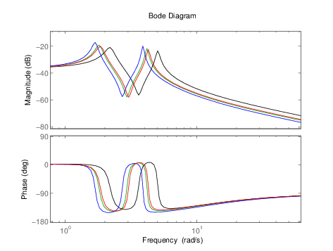
Figure 1 shows a detail of the Bode diagrams for m=0.5m=0.5 computed using the polynomial approximations of degree zero (black), one (blue) and two (red), together with the exact reduced system (green). It is clearly seen that the results improve as the order of the polynomial approximation is increased. Notice that the zeroth order polynomial approximation is equivalent to considering m=0m=0.

Refer to caption
Fig. 1: Comparison of Bode plots for zeroth (black), first (blue) and second (red) order approximations for m=0.5m=0.5, together with the exact reduction of the system (green).

V CONCLUSIONS

We have developed a parameter dependent model order reduction algorithm based on the balanced realization approximation. The algorithm yields a reduced order model which can be used to design a controller valid for a range of values of the parameter. As a by-product, we have obtained an expression for the second order perturbation of the singular subspaces (see equations (102) or (103)).

We should point out that, from the point of view of simulating a large system, it may be better to compute the exact reduced system for a given value of the parameter, since the truncation error of our second order polynomial approximation may become quite large for large mm (or even yield unstable reduced systems). Our procedure is thus more relevant for control design than for simulation.

Some trivial extensions of our work, which we have not reported here for the sake of simplicity, include considering several parameters instead of one or computing some further higher order corrections of the parametrized SVD.

We have not addressed the issue of the estimation of the error of the reduced model. Notice that this error involves both the truncation errors of the different steps of the algorithm and the error which comes from the truncation of the balanced realization. The latter is the only present for m=0m=0, and is the one for which bounds are well known. We currently do not know how to deal with the former, and how it could be integrated with the latter. However, the simulations of the system that we have presented, together with some simulations of the individual steps (not reported here) seem to indicate that the errors due to the different polynomial truncations go down when higher order approximations are used. We plan to address this issue by relating our construction to the general framework of [3] (see also [2]), and by comparing it to the approaches in [4].

Our algorithm has an important limitation, namely that it can only be applied to stable systems. Application of coprime factorization techniques for parameter dependent systems [12], which we plan to do in the future, could remove this drawback.

Acknowledgements

CB partially supported by the Generalitat de Catalunya through project 2014 SGR 267 and by the Spanish government through DPI2015-69286-C3-2-R (MINECO/FEDER). The authors would like to thank Yu. O. Vorontsov and Kh. D. Ikramov for making the Matlab code for their ABST algorithm available to them.

References

  • [1] A. C. Antoulas. Approximation of large-scale dynamical systems. Advances in Design and Control. Society for Industrial and Applied Mathematics, 2005.
  • [2] C. L. Beck. Model reduction and minimality for uncertain systems. PhD thesis, California Institute of Technology, 1996.
  • [3] C. L. Beck, J. Doyle, and K. Glover. Model reduction of multidimensional and uncertain systems. IEEE Transactions on Automatic Control, 41(10):1466–1477, 1996.
  • [4] P. Benner, S. Gugercin, and K. Willcox. A Survey of Projection-Based Model Reduction Methods for Parametric Dynamical Systems. SIAM Review, 57(4):483–531, 2015.
  • [5] D. F. Enns. Model reduction with balanced realizations: An error bound and a frequency weighted generalization. In Decision and Control, 1984. The 23rd IEEE Conference on, pages 127–132. IEEE, 1984.
  • [6] K. Glover. All Optimal Hankel-norm Approximations of Linear Multivariable Systems and their L-infinity Error Bounds. International Journal of Control, 39(6):1115–1193, 1984.
  • [7] A. J. Laub, M. T. Heath, C. C. Paige, and R. C. Ward. Computation of System Balancing Transformations and Other Applications of Simultaneous Diagonalization Algorithms. IEEE Transactions on Automatic Control, AC-32(2):115–122, 1987.
  • [8] Jun Liu, X. Liu, and Xiaoli Ma. First-Order Perturbation Analysis of Singular Vectors in Singular Value Decomposition. IEEE Transactions on Signal Processing, 56(7-1):3044–3049, 2008.
  • [9] Ha Binh Minh, C. Batlle, and E. Fossas. A new estimation of the lower error bound in balanced truncation method. Automatica, 50:2196–2198, 2014.
  • [10] B. C. Moore. Principal Component Analysis in Linear Systems: Controllability, Observability, and Model Reduction. IEEE Transactions on Automatic Control, AC-26(1):17–32, 1981.
  • [11] M. R. Opmeer and T. Reis. A Lower Bound for the Balanced Truncation Error for MIMO Systems. IEEE Trans. Automat. Contr., 60(8):2207–2212, 2015.
  • [12] E. Prempain. On Coprime factors for Parameter-Dependent Systems. In Proceedings of the 45th IEEE Conference on Decision and Control, pages 5796–5800. IEEE, 2006.
  • [13] J. M. A. Scherpen. Balancing for Nonlinear Systems. Systems & Control Letters, 21:143–153, 1993.
  • [14] W. H. A. Schilders, H. A. van der Vorst, and Joost Rommes, editors. Model order reduction: theory, research aspects and applications, volume 13 of Mathematics in industry; The European Consortium for Mathematics in Industry. Elsevier, 2008.
  • [15] G. W. Stewart. Perturbation theory for the singular value decomposition. SVD and Signal Processing, II: Algorithms, Analysis and Applications, pages 99–109, 1991.
  • [16] E. Verriest. Time variant balancing and nonlinear balanced realizations. In Wilhelmus H. A. Schilders, Henk A. van der Vorst, and Joost Rommes, editors, Model order reduction. Theory, research aspects and applications. Springer, 2008.
  • [17] E. Verriest and T. Kailath. On generalized balanced realizations. Automatic Control, IEEE Transactions on, 28(8):833–844, aug 1983.
  • [18] Yu O Vorontsov and Kh D Ikramov. A numerical algorithm for solving the matrix equation AX+ X T B= C 1. Computational Mathematics and Mathematical Physics, 51(5):691–698, 2011.