Nonlinear response of the quantum Hall system to a strong electromagnetic radiation

Integer quantum Hall effect (QHE) is remarkable phenomenon of two dimensional electron gas (2DEG) systems, in which the longitudinal resistance vanishes while the Hall resistance is quantized into plateaus [1]. The static QHE is the hallmark of dissipationless topological quantum transport [2] and despite its long history there is a continuing enormous amount of interest on this effect along various avenues. With the advent of new materials, such as graphene and topological insulators new regimes of QHE have been revealed [3, 4]. While static properties of the integer QHE have been well investigated in the scope of linear response theory, the dynamic and nonlinear responses in the quantum Hall system (QHS) in the high-frequency regime are not fully explored. In Ref. [5] considering the quantum dynamics of QHS exposed to an intense high-frequency electromagnetic wave, it is shown that the wave decreases the scattering-induced broadening of Landau levels. Linear response of the QHS in the high-frequency regime has been theoretically examined in Ref. [6]. As was shown in Ref. [6] the plateau structure in the QHS is retained, up to significant degree of disorder, even in the THz regime, although the heights of the plateaus are no longer quantized. Then this effect has been confirmed experimentally in Ref. [7]. Thus, a problem remains as how QHS responded to a strong and high-frequency electromagnetic wave fields, which is the purpose of the present study. In this case it is of interest to study generation of harmonics [8, 9] at the interaction of a strong pump wave with the Landau quantized 2DEG.

In the QHS wave-particle interaction can be characterized by the dimensionless parameter $\chi=eE_{0}l_{B}/(\hbar\omega)$, which represents the work of the wave electric field $E_{0}$ on the magnetic length $l_{B}=\sqrt{c\hbar/(eB)}$ ($e$ is the elementary charge, $\hbar$ is Planck’s constant, $c$ is the light speed in vacuum, and $B$ is the magnetic field strength) in units of photon energy $\hbar\omega$. The linear response theory is valid at $\chi<<1$. At $\chi\sim 1$ multiphoton effects become considerable. In this paper we consider just multiphoton interaction regime and look for features in the harmonic spectra of the strong wave driven QHS. As a 2DEG system we consider GaAs/AlGaAs single heterojunction. The time evolution of the considered system is found using a nonperturbative numerical approach, revealing that the generated in the QHS harmonics’ radiation intensity has a characteristic Hall plateaus feature. The effect remains robust against a significant broadening of Landau levels and takes place for wide range of intensities and frequencies of a pump wave.

We begin our study with construction of the single-particle Hamiltonian which defines the quantum dynamics of considered QHS. The 2DEG is taken in the $xy$ plane ($z=0$) and a uniform static magnetic field is applied in the $\mathrm{OZ}$ direction. We consider an incoming electromagnetic radiation pulse $E(t-z/c)$ propagating in the $\mathrm{OZ}$ direction and linearly polarized along the x axis. The incoming wave is assumed to be quasimonochromatic of carrier frequency $\omega$ and slowly varying envelope $E_{0}(t)$. For the 2DEG as realized in GaAs/AlGaAs we have uniform time-dependent electric field $E(t)=E_{0}(t)\sin\omega t$ and the single-particle Hamiltonian of QHS reads:

$$\mathcal{H}_{s}=\hbar\omega_{B}\left(\widehat{a}^{\dagger}\widehat{a}+\frac{1}{2}\right)+\left[\frac{el_{B}E(t)}{\sqrt{2}}\left(\widehat{b}+i\widehat{a}\right)+\mathrm{h.c.}\right].$$

(1)

Here $\omega_{B}=eB/\left(m^{\ast}c\right)$ is the cyclotron frequency, $m^{\ast}=0.068m_{e}$ is the effective mass ($m_{e}$ - the bare electron mass). For the interaction Hamiltonian we use a length gauge describing the interaction by the potential energy. The ladder operators $\widehat{a}$ and $\widehat{a}^{\dagger}$ describe quantum cyclotron motion, while $\widehat{b}$ and $\widehat{b}^{\dagger}$ correspond to guiding center motion. These ladder operators satisfy the usual bosonic commutation relations $[\widehat{a},\widehat{a}^{\dagger}]=1$ and $[\widehat{b},\widehat{b}^{\dagger}]=1$. The single free particle Hamiltonian, that is the first term in Eq. (1) can be diagonalized analytically. The wave function and energy spectrum are given by:

$$|\psi_{n,m}\rangle=|n,m\rangle,$$

(2)

$$\varepsilon_{n}=\hbar\omega_{B}\left(n+\frac{1}{2}\right).$$

(3)

Here $|n,m\rangle\ =|n\rangle\ \otimes|m\rangle$, with $|n\rangle$ and $|m\rangle$ being the harmonic oscillator wave functions. The eigenstates (2) are defined by the quantum numbers $n,m=0,1...$. Here $n$ is the LL index. The LLs are degenerate upon second quantum number $m$ with the degeneracy factor $N_{B}=\mathcal{S}/2\pi l_{B}^{2}$ which equals the number of flux quanta threading the 2D surface $\mathcal{S}$ occupied by the 2DEG. The terms $\sim\widehat{a}E(t)$ in the Hamiltonian (1) describe transitions between LLs, while the terms $\sim\widehat{b}E(t)$ describe transitions within the same LL. These transitions can be excluded from the consideration by the appropriate dressed states for the construction of the carrier quantum field operators. Expanding the fermionic field operator

$$|\widehat{\Psi}\rangle=\sum\limits_{n,m}\widehat{a}_{n,m}|\widetilde{\psi}_{n,m}\rangle$$

(4)

over the dressed states

$$|\widetilde{\psi}_{n,m}\rangle=\exp\left[-\frac{i}{\hbar}\frac{el_{B}}{\sqrt{2}}\int_{0}^{t}E(t^{\prime})dt^{\prime}\left(\widehat{b}^{\dagger}+\widehat{b}\right)\right]|\psi_{n,m}\rangle,$$

(5)

the Hamiltonian of the system in the second quantization formalism

$$\widehat{H}=\left\langle\widehat{\Psi}\right|\mathcal{H}_{s}\left|\widehat{\Psi}\right\rangle$$

can be presented in the form:

$$\widehat{H}=\sum\limits_{n=0}^{\infty}\sum\limits_{m=0}^{N_{B}}\varepsilon_{n}\widehat{a}_{n,m}^{+}\widehat{a}_{n,m}+\sum\limits_{n,n^{\prime}=0}^{\infty}\sum\limits_{m=0}^{N_{B}}E(t)\mathcal{D}_{n,n^{\prime}}\widehat{a}_{n,m}^{+}\widehat{a}_{n^{\prime},m},$$

(6)

where $\widehat{a}_{n,m}^{\dagger}$ and $\widehat{a}_{n,m}$ are, respectively, the creation and annihilation operators for a carrier in a LL state, and $\mathcal{D}_{n,n^{\prime}}$ is the dipole moment operator:

$$\mathcal{D}_{n,n^{\prime}}=\frac{iel_{B}}{\sqrt{2}}\left[\sqrt{n-1}\mathbb{\delta}_{n-1,n^{\prime}}+\sqrt{n}\mathbb{\delta}_{n,n^{\prime}-1}\right]\frac{\hbar\omega_{B}}{\varepsilon_{n^{\prime}}-\varepsilon_{n}}.$$

Then we will pass to Heisenberg representation where operators obey the evolution equation

$$i\hbar\frac{\partial\widehat{L}}{\partial t}=\left[\widehat{L},\widehat{H}\right]$$

and expectation values are determined by the initial density matrix $\widehat{D}$: $<\widehat{L}>=Sp\left(\widehat{D}\widehat{L}\right)$. In order to develop microscopic theory of the nonlinear interaction of the QHS with a strong radiation field, we need to solve the Liouville-von Neumann equation for the single-particle density matrix

$$\rho(n_{1},m_{1};n_{2},m_{2},t)=<\widehat{a}_{n_{2},m_{2}}^{+}(t)\widehat{a}_{n_{1},m_{1}}(t)>$$

(7)

and for the initial state of the quasiparticles we assume an ideal Fermi gas in equilibrium:

$$\rho(n_{1},m_{1};n_{2},m_{2},0)=\frac{\delta_{n_{1},n_{2}}\delta_{m_{1},m_{2}}}{1+\exp\left(\frac{\varepsilon_{n_{1}}-\varepsilon_{F}}{T}\right)}.$$

(8)

Including in Eq. (8) quantity $\varepsilon_{F}$ is the Fermi energy, $T$ is the temperature in energy units. As is seen from the interaction term in the Hamiltonian (6) quantum number $m$ is conserved: $\rho(n_{1},m_{1};n_{2},m_{2},t)=\rho_{n_{1},n_{2}}\left(t\right)\delta_{m_{1},m_{2}}$. To include the effect of the LLs broadening we will assume homogeneous broadening of the LLs [10]. The latter can be incorporated into evolution equation for $\rho_{n_{1},n_{2}}\left(t\right)$ by the damping term $-i\Gamma_{n_{1},n_{2}}\rho_{n_{1},n_{2}}\left(t\right)$ and from Heisenberg equation one can obtain evolution equation for the reduced single-particle density matrix:

$$i\hbar\frac{\partial\rho_{n_{1},n_{2}}(t)}{\partial t}=\left[\varepsilon_{n_{1}}-\varepsilon_{n_{2}}\right]\rho_{n_{1},n_{2}}(t)-i\Gamma_{n_{1},n_{2}}\rho_{n_{1},n_{2}}\left(t\right)$$

$$-E(t)\sum\limits_{n}\left[\mathcal{D}_{n,n_{2}}\rho_{n_{1},n}(t)-\mathcal{D}_{n_{1},n}\rho_{n,n_{2}}(t)\right].$$

(9)

For the damping matrix we take $\Gamma_{n_{1},n_{2}}=\Gamma\left(1-\delta_{n_{1},n_{2}}\right)$, where $\Gamma$ measures the LL broadening.

Solving Eq. (9) with the initial condition (8) one can reveal nonlinear response of the QHS to a strong radiation pulse. At that one can expect intense radiation of harmonics of the incoming wave-field in the result of the coherent transitions between LLs. The harmonics will be described by the additional generated fields $E_{x,y}^{(g)}$. We assume that the generated fields are considerably smaller than the incoming field $\left|E_{x,y}^{(g)}\right|<<\left|E\right|$. In this case we do not need to solve self-consistent Maxwell’s wave equation with Heisenberg equations. To determine the electromagnetic field of harmonics we can solve Maxwell’s wave equation in the propagation direction with the given source term:

$$\frac{\partial^{2}E_{x,y}^{(t)}}{\partial z^{2}}-\frac{1}{c^{2}}\frac{\partial^{2}E_{x,y}^{(t)}}{\partial t^{2}}=\frac{4\pi}{c^{2}}\frac{\partial\mathcal{J}_{x,y}\left(t\right)}{\partial t}\delta\left(z\right).$$

(10)

Here $\delta\left(z\right)$ is the Dirac delta function and $\mathcal{J}_{x,y}$ is the mean value of the surface current density operator:

	$\displaystyle\widehat{\mathcal{J}}_{x}\left(t\right)$	$\displaystyle=$	$\displaystyle\frac{-2e\hbar}{\sqrt{2}l_{B}m^{\ast}\mathcal{S}}\left\langle\widehat{\Psi}\right|\left(\hat{a}^{\dagger}+\hat{a}\right)\left|\widehat{\Psi}\right\rangle,$
	$\displaystyle\widehat{\mathcal{J}}_{y}\left(t\right)$	$\displaystyle=$	$\displaystyle\frac{-2e\hbar}{i\sqrt{2}l_{B}m^{\ast}\mathcal{S}}\left\langle\widehat{\Psi}\right|\left(\hat{a}^{\dagger}-\hat{a}\right)\left|\widehat{\Psi}\right\rangle.$		(11)

With the help of Eqs. (4) and (7) the expectation value (11) of the total current in components can be written in the following form:

$$\mathcal{J}_{x}\left(t\right)=j_{0}\sum\limits_{n=0}\sqrt{n+1}\mathrm{Re}\rho_{n,n+1}\left(t\right),$$

$$\mathcal{J}_{y}\left(t\right)=-j_{0}\sum\limits_{n=0}\sqrt{n+1}\mathrm{Im}\rho_{n,n+1}\left(t\right),$$

(12)

where $j_{0}=-\sqrt{2}e\hbar/\left(\pi l_{B}^{3}m^{\ast}\right)$ (here we have taken into account the spin degeneracy factor). The solution to equation (10) reads

$$E_{x,y}^{(t)}\left(t,z\right)=E_{x,y}\left(t-z/c\right)$$

$$-\frac{2\pi}{c}\left[\theta\left(z\right)\mathcal{J}_{x,y}\left(t-z/c\right)+\theta\left(-z\right)\mathcal{J}_{x,y}\left(t+z/c\right)\right],$$

(13)

where $\theta\left(z\right)$ is the Heaviside step function with $\theta\left(z\right)=1$ for $z\geq 0$ and zero elsewhere. The first term in Eq. (13) is the incoming wave. In the second line of Eq. (13), we see that after the encounter with the 2DEG two propagating waves are generated. One traveling in the propagation direction of the incoming pulse and one traveling in the opposite direction. The Heaviside functions ensure that the generated light propagates from the source located at $z=0$. We assume that the spectrum is measured at a fixed observation point in the forward propagation direction. For the generated field at $z>0$ we have

$$E_{x,y}^{(g)}\left(t-z/c\right)=-\frac{2\pi}{c}\mathcal{J}_{x,y}\left(t-z/c\right).$$

(14)

Now, performing the summation in Eqs. (12) and using solutions (14) we can calculate the harmonic radiation spectrum with the help of Fourier transform of the functions $E_{x,y}^{(g)}\left(t-z/c\right)$:

$$E_{x,y}^{(g)}\left(s\right)=\frac{\omega}{2\pi}\int_{0}^{2\pi/\omega}E_{x,y}^{(g)}\left(t\right)e^{is\omega t}dt.$$

(15)

The spectrum contains in general both even and odd harmonics. However, depending on the initial conditions, in particular, for the equilibrium initial state (8) the terms containing even harmonics cancel each other because of inversion symmetry of the system and only the odd harmonics are generated. The time evolution of system (9) is found with the help of the standard fourth-order Runge-Kutta algorithm and for calculation of the power spectra the fast Fourier transform algorithm is used. To avoid nonphysical effects semi-infinite pulses with smooth turn-on, in particular, with hyperbolic tangent $tanh(t/\tau_{r})$ envelope is considered. Here the characteristic rise time $\tau_{r}$ is chosen to be $\tau_{r}=10\pi/\omega$.

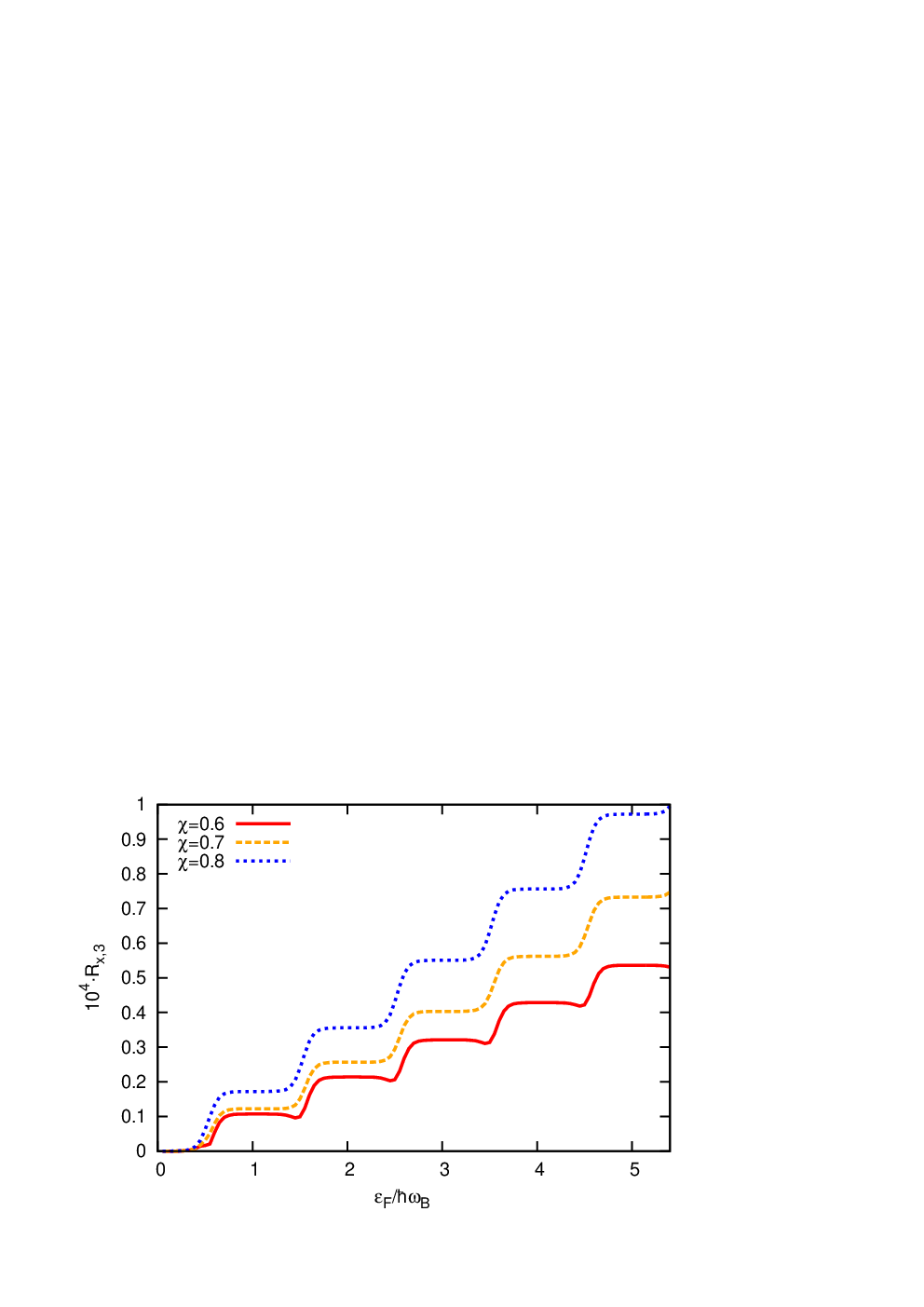
Figures 1 and 2 show nonlinear response of the QHS via normalized harmonics field strengths versus Fermi energy for various pump wave intensities. Here and below the temperature is taken to be $T/\hbar\omega_{B}=0.05$. Figure 1 displays normalized field strength at the fundamental harmonic $R_{y,1}=\left|E_{y}^{(g)}\left(1\right)\right|/E_{0}$ polarized perpendicular to the polarization of a pump wave, while Fig. 2 displays the third harmonic field strength $R_{x,3}=\left|E_{x}^{(g)}\left(3\right)\right|/E_{0}$. From these figures we immediately notice a step-like structure of the nonlinear response of the QHS system as a function of $\varepsilon_{F}$ for various pump wave intensities. Although the step heights are not quantized exactly, the flatness, which is a intrinsic property of the static QHE, surprisingly exists also in the nonlinear response of the QHS. In the static QHE the step structure of the Hall conductivity is a quantum and topological effect. In the considered case Eqs. (12) does not simply reduce to a topological expression and the result for the robust plateaus of the nonlinear optical response is not apparent.

We further examine how the step-like structure in the nonlinear response of the QHS behaves for various pump wave frequencies. The generated fields versus Fermi energy and pump wave frequency at the fundamental and third harmonics are shown in Figs. 3 and 4. Thus, the step structure preserves for the wide range of the pump wave frequencies.

We also investigate how the step-like structure in the nonlinear response of the QHS behaves as we vary the LL broadening. So we have calculated $R_{y,1}$ as a function of $\Gamma$, for fixed values of $\omega$ and $\chi$. We can see from Fig. 5 that, while the density of states broadens with a width $\sim\Gamma$ the step structure remains up to large $\Gamma$.

Finally let us consider the experimental feasibility. It is clear that in experiment one can observe the considered effect by measuring $R_{y,1}$ and/or $R_{x,3}$. The first quantity is responsible for the nonlinear Faraday effect, while last quantity responsible for third harmonic radiation polarized along the incoming wave polarization. Thus, the step structure should be observed as jumps in the intensity of third harmonic or fundamental harmonic radiation with orthogonal polarization. The magnetic field strength is assumed to be $B=3\ T$. For the incoming wave field we will assume $\hbar\omega\simeq 3.5\ \mathrm{meV}$. The intensity of the incoming wave for $\chi=0.8$ is $4.\,\allowbreak 4\times 10^{3}$ $\mathrm{W/cm}^{2}$. For the setup of Fig. 1 the steps in the Faraday-rotation angle $\Delta\Theta_{F}\sim R_{y,1}\sim 10\ \mathrm{mrad}$, which is well within the experimental resolution [11]. For the setup of Fig. 2 with the chosen parameters the average intensity of the third harmonic radiation is $I_{3}\sim 2.\,\allowbreak 2\times 10^{-5}$ $\mathrm{W/cm}^{2}$ (corresponding to $10^{16}$ $\mathrm{photons/s\cdot cm}^{2}$) with the steps $\Delta I_{3}\sim 0.36\times I_{3}$.

To summarize, we have presented a microscopic theory of the 2DEG interaction with coherent electromagnetic radiation in the quantum Hall regime. The evolutionary equation for a single-particle density matrix has been solved numerically. We have revealed that the nonlinear optical response of QHS to an intense radiation pulse, in particular, radiation intensity at the harmonics, as well as nonlinear Faraday effect, has a characteristic Hall plateau structures that persist for a wide range of the pump wave frequencies and intensities even for significant broadening of LLs.

This work was supported by the RA MES State Committee of Science, in the frames of the research project No. 15T-1C013.

References

- [1] K. v. Klitzing, G. Dorda, and M. Pepper, Phys. Rev. Lett. 45 (1980) 494.
- [2] D. J. Thouless, M. Kohmoto, M. P. Nightingale, and M. den Nijs, Phys. Rev. Lett. 49 (1982) 405
- [3] K. S. Novoselov et al., Nature 438 (2005) 197.
- [4] R. Yoshimi et al., Nat. Commun. 6 (2015) 6627.
- [5] K. Dini, O. V. Kibis, and I. A. Shelykh, arXiv:1603.04965 (2016).
- [6] T. Morimoto, Y. Hatsugai, and H. Aoki, Phys. Rev. Lett. 103 (2009) 116803.
- [7] Y. Ikebe, T. Morimoto, R. Masutomi, T. Okamoto, H. Aoki, and R. Shimano, Phys. Rev. Lett. 104 (2010) 256802.
- [8] H. K. Avetissian, A. K. Avetissian, G. F. Mkrtchian, Kh. V. Sedrakian, Phys. Rev. B 85 (2012) 115443.
- [9] H. K. Avetissian, A. K. Avetissian, G. F. Mkrtchian, Kh. V. Sedrakian, J. Nanophoton. 6 (2012) 061702.
- [10] T. Dittrich, P. Haengi, G.-L. Ingold, B. Kramer, G. Schoen and W. Zwerger, Quantum Transport and Dissipation, Wiley-VCH, 1998.
- [11] Y. Ikebe and R. Shimano, Appl. Phys. Lett. 92 (2008) 012111.