Distributed rotational and translational maneuvering of rigid formations and their applications.
Abstract
Recently it has been reported that range-measurement inconsistency, or equivalently mismatches in prescribed inter-agent distances, may prevent the popular gradient controllers from guiding rigid formations of mobile agents to converge to their desired shape, and even worse from standing still at any location. In this paper, instead of treating mismatches as the source of ill performance, we take them as design parameters and show that by introducing such a pair of parameters per distance constraint, distributed controller achieving simultaneously both formation and motion control can be designed that not only encompasses the popular gradient control, but more importantly allows us to achieve constant collective translation, rotation or their combination while guaranteeing asymptotically no distortion in the formation shape occurs. Such motion control results are then applied to (a) the alignment of formations’ orientations and (b) enclosing and tracking a moving target. Besides rigorous mathematical proof, experiments using mobile robots are demonstrated to show the satisfying performances of the proposed formation-motion distributed controller.
Index Terms:
Formation Control, Rigid Formation, Motion Control, Target enclosing.I Introduction
Many coordinated robot tasks, such as, the enclosing of a target [1], area exploration & surveillance [2] and the vehicle platooning for energy efficiency [3], can be achieved by combining two different cooperative controls: multi-agent formation control and group motion control. The former is to achieve and maintain a specific desired shape of a multi-agent formation while the latter to guide the motion of the group as a whole. For simple formations, such as, line formations in the vehicle platooning problem, these two control problems can be solved simultaneously by using the passivity-based control approach as pursued in [4]. However, for formations in more complicated shapes, these two control problems are usually tackled separately, namely using the gradient-based strategies for formation control and leader-follower coordination for motion control, where for the latter the leader moves according to a desired trajectory and the followers simply track the leader [5]. But when the separately designed formation controller and motion controller are jointly in force as in the common scenario in practice, conflict often occurs: the shape of the formation is distorted when an agent compromises between the demands from formation and motion controls as to where and how it needs to move [6, 7]. While efforts have been made before to solve such conflict by installing velocity sensors in addition to position sensors on mobile agents and thus compensating the distortion with the help of the more sensed information [5], we in this paper take a much more head-on approach by generalizing the gradient-based distributed formation control law for both control objectives simultaneously guaranteeing no shape distortion in the steady-state desired formation motion even without the knowledge of any additional sensed information in comparison to the conventional control. The surprisingly simple structure of our proposed control law opens possibilities to solve other difficult problems, such as, collective rotational motion, the enclosing of a moving target and the formation coordination task for agents governed by higher-order dynamics.
In gradient-based formation control, stabilizable formations are identified employing rigidity graph theory where the vertices of a graph represent the agents and the edges stand for the inter-agent distance constraints to define the shape of the formation [8, 9, 10, 11]. Rigid formations are associated with a potential function determined by the agents’ relative positions. The potential has a minimum at the desired distances between the agents and thus its gradient leads naturally to the formation controller that stabilizes rigid formations locally. However, it was recently reported in [12] and later more exhaustively studied in [13, 14] that for such control laws, if there are mismatches between the prescribed distances for neighboring agents, the performance of the controller deteriorates significantly since mismatches induce undesired steady-state motion and distortion in the formation shape. If no estimators, as proposed and experimented in [15], are installed to improve the performance of such controllers, the mismatch-induced motion in steady-states takes interesting forms for almost all mismatches: in , the formation follows a closed orbit with a constant angular velocity; in the movement is helical, determined by a single sinusoidal signal and a constant drift [16].
Motivated by the mismatch-induced motion reported in [16], we introduce parameter pairs in the gradient-based formation control law for steering the whole formation; in particular, for each prescribed distance constraint, we introduce a pair of motion parameters, mimicking the mismatches as studied in [16]. By a one-step (centralized) systematic design of such motion parameters, we show that we can steer the entire formation in rotation and/or translation in a distributed manner. The proposed gradient-based formation-motion joint controller using the motion parameters has several advantages. First, one can achieve precisely the desired steady-state formation shape and the group motion simultaneously, including rotational motion, in a distributed fashion. To the best of our knowledge, no such result has been reported in the literature. For single-integrator agent dynamics, we relate analytically the magnitude of the motion parameters to the speed of the group motion. Second, our proposed approach enables us to align the formation with respect to a global coordinate frame by adding a simple control term to an arbitrary agent when guiding the group in motion. In comparison, in the literature such an alignment is usually obtained by assigning a leader who knows the global frame and letting the other agents (followers) estimate the leader’s velocity employing a distributed estimator [5]. Obviously in our approach, such estimators are not needed at all. Third, one can easily use our method to address the target tracking and enclosing problem both in and where one assigns the formation shape to specify how the target is enclosed and tracked by the pursuers. In comparison to the solution of such problems in [17, 18] among other works, we do not confine our formation to follow the same circular trajectory nor require all enclosing agents to measure their relative positions with respect to the target. The rest of the paper is organized as follows. In Section II we introduce the notation and background for rigid formations in and and we briefly review the gradient control in Section III. The design of the desired steady state motion with the desired formation shape is described in Section IV, while the corresponding stability analysis is presented in Section V. We implement our proposed formation-motion controller in two different contexts: (i) the design of a simultaneous formation & translation control in global coordinates in Section VI-A; and (ii) the formation control design for solving the target tracking and enclosing problem in Section VI-B. Finally experimental results using wheeled mobile robots are shown in Section VII.
II Preliminaries
In this section, we introduce some notations and basic concepts. For a given matrix , define , where the symbol denotes the Kronecker product, for or otherwise for , and is the -dimensional identity matrix. For a stacked vector with , we define the diagonal matrix . We denote by the cardinality of the set and by the Euclidean norm of a vector . We use and to denote the all-one and all-zero matrix in respectively.
II-A Formations and graphs
We consider a formation of autonomous agents whose positions are denoted by . The agents are able to sense the relative positions of its neighboring agents. The neighbor relationships are described by an undirected graph with the vertex set and the ordered edge set . The set of the neighbors of agent is defined by . We define the elements of the incidence matrix for by
where and denote the tail and head nodes, respectively, of the edge , i.e. . A framework is defined by the pair , where is the stacked vector of the agents’ positions . The stacked vector of the sensed relative distances can then be described by
Note that each vector in corresponds to the relative position associated with the edge .
II-B Infinitesimally and minimally rigid formations and their realization
In this section we will briefly review the concept of rigid formations and how to design them. Most of the concepts explained here are covered in much more detail in [19] and [20]. Define the edge function by and denote its Jacobian by , which is called in the literature the rigidity matrix. A framework is infinitesimally rigid if when embedded in or if when it is embedded in . Additionally, if in the 2D case or in the 3D case then the framework is called minimally rigid. Roughly speaking, under the distance contraints the only motions that one can perform over the agents in an infinitesimally and minimally rigid framework, while they are already in the desired shape, are the ones defining translations and rotations of the whole shape. We illustrate in Figure 1 some examples in and of rigid and non-rigid frameworks.
For a given stacked vector of desired relative positions , the resulting set of the possible formations is defined by
where is the set of rotational matrices in or . Roughly speaking, consists of all formation positions that are obtained by rotating . If is infinitesimally and minimally rigid, then, similar to the above, we can define the set of resulting formations by
where .
Note that in general it holds that . For a desired shape, one can always design to make the formation infinitesimally and minimally rigid. In fact in , an infinitesimally and minimally rigid framework with two or more vertices can always be constructed through the Henneberg construction [21]. Unfortunately there is no known corresponding systematic operations in yet. Nevertheless in one can always obtain an infinitesimally and minimally rigid framework by the Henneberg-like tetrahedron insertions as it has been done in [15].
III Gradient control in inter-agent distances
For a formation of agents associated with the neighbor relationship graph , consider the following system where we model the agents as kinematical points
| (1) |
where is the stacked vector of control inputs for .
For each edge one can construct a potential function with its minimum at the desired distance so that the gradient of such functions can be used to control inter-agent distances distributively.
We take as a potential function
and apply to each agent in (1) the following gradient descent control
| (2) |
One can then show straightforwardly that the multi-agent formation will converge locally to the desired shape employing the following known results.
Theorem III.1
The authors of [22, 23] have shown that for a real analytic potential function , system (1) with the control law (2) is locally asymptotically stable about the point corresponding to the local minima of . We consider for each edge the following family of quadratic11 1 Any analytic potential functions, including the ones for collision avoidance [24], can be approximated by a quadratic function in a small neighborhood about their local minima, and for this reason such quadratic potentials are of special interest of study. potential functions
| (3) |
with the following gradient along
| (4) |
One immediate observation is that when , the right-hand side of (4) becomes the unit vector multiplied by the distance error . This fact will play an important role later for the design of the desired steady-state motion of the formation. It is straightforward to check that for every edge one has , and obviously for all . Thus the agent dynamics (1) under (2) can be written in the following compact form
| (5) |
where is the stacked vector of ’s. Denoting the distance error for edge by
| (6) |
it follows that
By substituting it into (5) and noting that
we can write down the closed-loop system dynamics in the compact form
| (7) | ||||
| (8) | ||||
| (9) |
where is the stacked vector of ’s, is the stacked column vector consisting of all the ’s, and the matrices and are the block diagonal matrices of and respectively, as defined before in Section II-A. In the following proposition, we establish the local exponential convergence of the error (6) to zero for arbitrary . This fact is a straightforward extension of the result in [13] for the case when , and we provide the proof below for completeness.
Proposition III.2
Proof:
First we prove that the error system (9) is autonomous. The elements of are products of the form . It has been shown in [14] that for any infinitesimally and minimally rigid framework, there exists a neighborhood about this framework such that any , can be written as a smooth function , and since , we can write
| (10) |
Thus the vector and the matrix can be rewritten as smooth functions depending locally only on about the origin. This shows that the error system (9) is at least locally an autonomous system.
Now to prove the stability of for (9), we choose a Lyapunov function which satisfies
Since and are positive definite matrices at the desired formation shape as has full row rank at , the matrix
| (11) |
is positive definite at . Since the eigenvalues of are smooth functions of , there exists a compact set
| (12) |
for some positive constant where is positive definite. Define to be the smallest eigenvalue of in . Then
| (13) |
which immediately implies the local exponential convergence of to zero. ∎We want to emphasize that as does not imply but instead . As pointed out by Theorem III.1, is guaranteed to converge to only when the initial condition is sufficiently close to .
IV Gradient-based formation-motion control
For the sake of simplicity and clarity in the notation, from this point onwards we will consider the case for and the main results can be easily extended to any . Then and thus is the identity matrix. We denote by the global frame of coordinates fixed at the origin of with some arbitrary fixed orientation. Similarly we denote by the local frame for agent with some fixed arbitrary orientation independent of . Finally, we denote by the body frame fixed at the centroid of the desired rigid formation. Furthermore, if we rotate the rigid formation with respect to , then is also rotated in the same manner. Let denote the position of agent with respect to . To simplify notation whenever we represent an agents’ variable with respect to , the superscript is omitted, e.g. .
We consider a pair of (scaled by a gain ) motion-control parameters and to the term for each agent associated with the edge . More precisely, agent uses a controlled distance and correspondingly, agent , . For the corresponding edge we incorporate these parameters to the gradient descent controller and apply the same gain , namely
where and are the corresponding control inputs for agents and with edge . The equations above lead to the following compact form
| (14) |
where the elements of are constructed in a very similar way as in the incidence matrix as follows
| (15) |
therefore we define as the stacked vectors of and for all . Note that if , then , which implies that we have a gradient-based control with being the new stacked vector of the prescribed distances. The gain is a free design parameter for achieving exponential stability of the formation as we will see later in the stability analysis.
One important property of (14) is that each agent can work with only its own local frame . One can see this more in detail in the following lemma.
Lemma IV.1
The control law applied in (14) can be implemented for each agent using only its local frame .
The proof is omitted due to space limitation but it is straightforward by following similar arguments as in [5, 11].
In order to induce some desired steady-state motion of the formation in the desired shape, we can manipulate and at the equilibrium of (14). Then the steady-state motion will be a function of the desired shape and :
| (16) |
Before discussing on how to design the motion parameters and in order to keep invariant, let us first recall some facts from rigid body mechanics [25]. As in the case of points in a rigid body, the steady-state velocity of every agent at the desired rigid formation shape can be decomposed into
| (17) |
where is the angular velocity of the rigid formation (similar to that for the rigid body). In particular, in view of (14) with as defined in (15), the velocity (17) at the desired shape is given by
| (18) |
Let us decompose the motion parameters into and , where and will be used to assign the desired translational and rotational velocity, respectively, of the rigid formation. Using this decomposition, we can rewrite (18) for all the agents into the following compact form
| (19) |
where is the stacked vector of all the rotational velocities .
In the desired shape, the stacked vector of relative positions in becomes a constant. This is due to the fact that follows the steady-state motion, and thus according to (19) the velocities and also become constant. In particular, if , then we will have a drift of the desired formation in ; otherwise for a nonzero constant vector , the formation will follow a closed circular orbit (which is always the case in 2D formations) when is perpendicular to , or otherwise a helical trajectory in . Figure 2 shows an illustration of these facts on the steady-state velocity of the desired formation expressed in either and .
Now we are ready to show how to design the motion parameters and in (19). Note that the steady-state motion must not distort the desired shape, i.e. the motion parameters have to be designed such that is an invariant set in (19). The desired steady-state velocity (16) in can be rewritten as
where is constructed from the incidence matrix setting its elements to zero and . The motion parameters will be used to design both velocities in (19) with respect to as in Figure 2c since they are constant in such a frame. Note that the knowledge about is only needed during the design stage for the desired steady-state velocity. During the implementation of the distributed control law, the agents only need to know about their own ’s as shown in Lemma IV.1.
We now demonstrate how to design the velocity employing the motion parameters. It is important to note that in an infinitesimally and minimally rigid framework, the minimum number of edges associated to a node is two in or three in . So if then the relative positions ’s associated to agent can span the whole for the planar formations (or in the 3D case). This implies that the domain of the desired velocity is the whole space and it can be assigned by an appropriate choice of and (c.f. (18)). Since the velocity is the same for all the agents, we set the following requirement for and
| (20) |
which implies that . However, since in general the kernel of can be non-trivial, there may exist non-zero such that , which is irrelevant for our motion control. Taking this into account, the set of motion parameters and should satisfy
| (21) |
where stands for the projection over the space . The lower bound for the degrees of freedom of choosing the elements of and for constructing can obviously be given by the number of motion parameters of the agent that has the least number of neighbors. In other words,
| (22) |
where is defined in Section II-A and in (21). Consequently, we propose the following algorithm to compute and for given and .
Algorithm IV.2
- 1.
Choose an agent with the least number of neighbors.
- 2.
Assign and associated to agent that solves .
- 3.
Compute a basis that spans the space defined in (21).
- 4.
Compute a vector employing the basis such that the previously computed ’s and ’s are the ’th and ’th elements of . Then, the rest of elements of are necessarily the motion parameters defining for the whole formation, i.e. .
From (15) it is clear that the implementation of the motion parameters is distributed, while the computation in Algorithm IV.2 is centralized since it requires the knowledge of and . On the other hand, the motion parameters only need to be computed once since the desired speed of the motion can be modified by just rescaling and . For a new agent joining the formation, its corresponding motion parameters for the translational motion can be computed in a distributed way. Consider agent joins the formation: if it asks a neighboring agent about and , then it becomes straightforward for agent to compute the corresponding motion parameters for the desired by only following the second step of Algorithm IV.2.
Now we proceed to show how to design the motion parameters for the rotational velocity in (19), i.e. the rotational motion of the agents around the centroid. Note that this rotational motion preserves the constant norms ’s but not the relative positions ’s. Since , we can impose the following condition for maintaining constant ,
| (23) |
As discussed after equation (19) the relative positions are constant because is rotating with the rigid formation. However, for having such rotation of the formation, the constant velocities must be designed in order to keep the norms ’s constant. Therefore, we impose the following restricting condition for and in addition to (23)
| (24) |
As in the case for calculating the motion parameters for , the set of motion parameters and are the subset of motion parameters such that
| (25) |
where is as in (21). We remark that the dimension of in (25) is at least, one less than the dimension of in (21). This is due to the fact is perpendicular to (as shown in (17)) and hence, the degree-of-freedom for choosing is at least one less than that for choosing . The calculation of the motion parameters and for a desired can be done in a similar way to Algorithm IV.2, where in the second step we assign the ’s giving the constant linear velocity for making the agent to rotate with angular velocity around the centroid derived from , and the basis in the third step is replaced by spanning as in (25).
As before the implementation of and is fully distributed but their computation at the design stage is not. On the other hand, they only need to be computed once and the angular speed can be regulated by just rescaling their magnitude. Note that for designing different trajectories in as in Figure 2, we only need to change the speed of and . Unfortunately, if a new agent joins the formation, then the centroid will change, requiring to recompute in a centralized way and . Nevertheless, if the instantaneous center of rotation [25] is independent of the new agent, e,g, as we will see in the target enclosing problem where it will be fixed at agent , then agent can still compute its motions parameters by only asking local information from a neighboring agent , i.e. its and along with and in addition we also require agent to know about .
Example IV.3
We would like to highlight the particular example of calculating the bluemotion parameters for triangular formations and its extension to tetrahedra in 3D. Consider a generic triangular formation consisting of three agents whose has the following incidence matrix
| (26) |
Then it can be checked that the following conditions for and (any four implying the remaining one)
| (27) |
satisfy (21) and they have a non-trivial solution with two degrees of freedom satisfying (22). We would like to emphasize that the set of equations in (27) is independent of . In general, the computation of and depends on as it is shown in the following proposition
Proposition IV.4
If defines an equilateral triangle, then
If defines an isosceles triangle with , then
| (28) |
with being a normalizing factor and defining the angular speed.
We omit the proof due to space constraint. Another interesting property is that the centroid of the triangular formation is invariant if and belong to (25) since
These results can be extended in a similar way to tetrahedrons.
V Stability analysis
After we have the design of the desired steady-state behavior of the formation as discussed thoroughly in Section IV, we provide the stability analysis of the closed-loop system in this section. In particular we show that the control law applied in (14), with designed as in Section IV, indeed steers the formation, at least locally, to the desired formation motion.
Similar to (8) and (9), we derive from (14) the following closed-loop system with the motion parameters
| (29) | ||||
| (30) |
Note that as shown in Proposition III.2, the error system (30) is autonomous since the elements of are linear combinations of the inner products . Therefore we can write (30) as
| (31) |
with as in (11) with and . Note that is closely related to the desired shape since implies . However, in general does not necessarily imply since
is designed to be zero only at but not at arbitrary .
Theorem V.1
There exist constants such that for system (31), corresponding to with the motion parameters and belonging to the spaces (21) and (25) respectively is locally exponentially stable for all in the compact set . In particular, the formation will converge exponentially to the shape defined by and the velocity will converge exponentially to for .
Proof:
We divide the proof in two parts. Firstly we analyze the inter-agent distance dynamics and show that the shape formed eventually by the agents is the desired shape. Secondly we analyze the individual agent dynamics in order to show that they converge to the steady-state motion defined by the motion parameters.
Consider the following candidate Lyapunov function
with its time derivative given by
As shown in Proposition III.2, there exists a constant such that is positive definite in the compact set since is positive definite as the framework is infinitesimally and minimally rigid at . Since is real analytic with at because of (20) and (24), it is also locally Lipschitz in . Therefore there exists a constant such that
| (32) |
where is the minimum eigenvalue of in . Thus if one chooses , then the local exponential stability of the origin of (31) follows, showing that the formation converges exponentially to the desired shape defined by .
For the second part of the proof, we substitute and as into (14), which gives us
In other words, the velocity of the agents converges exponentially to the desired velocities given by and for all . ∎
Example V.2
As before, triangles and tetrahedrons can be considered as particular cases. For triangles we can write
where and is given by
We would like to pinpoint two special cases. Firstly we notice that for and we have that is zero in (29) since . In this case, for all . Secondly, if defines an equilateral triangle, then is skew symmetric in view of Proposition IV.4. This means that for all in (32). Therefore both special cases have , and hence for any the origin of (30) is locally exponentially stable. As before, similar results can be easily extended to tetrahedrons.
It is important to note that we are assuming that the measurements done by the agents are not biased with respect to each other, i.e. we do not consider any undesired mismatches that will affect the performance of the motion controller. This is still an open issue that could be addressed in future works by exploiting the ideas contained in [15].
In the following section, we apply the motion parameters to a more specific applications of formation motion control.
VI Applications of employing only motion parameters
The results from Theorem V.1 allow one to design the behaviour of the steady-state motion of the desired formation. However, these results are restricted to the design of the velocities for all , which are obviously defined in . In particular, for the case of having only translational motion, i.e. , the steady-state orientation of with respect to is unknown and depends on the initial condition . Similarly, for the rotational motion around the centroid, i.e. , the steady-state position of the centroid of the formation also depends on .
Throughout the following two subsections, we are going to extend the results of Theorem V.1 in order to overcome the issues mentioned above. The first extension is concerned with the control of the steady-state orientation of with respect to in the special case of having only a translational motion. The second extension deals with the control of the instantaneous center of rotation for the formation, which is closely related to the problem of tracking and enclosing a target as briefly mentioned in the Introduction.
VI-A Translational motion with controlled heading
Suppose that the motion parameters have been assigned such that the steady-state motion of the formation defines a pure translation, i.e. . In this special case, we are interested in controlling the steady-state orientation of with respect to , and consequently the heading of the translational motion in . This task can be accomplished if we control only one relative position among all the ’s with respect to . Without loss of generality we set the relative position associated to edge for achieving this task. Since defines a rigid formation, if we control the orientation of then the orientation of the rest ’s will also be controlled. In other words, we are setting the desired orientation of the formation in with the following relation
| (33) |
where has the orientation with respect to given by the desired rotational matrix defining the steady-state orientation of with respect to .
Let us introduce the following potential function in order to settle the orientation controller for implemented by the agents in
| (34) |
and define the alignment error
The orientation controller derived from the gradient of (34) is
| (35) |
Note that we require agents and to know , since they will need for the computation of (35) in . Let us introduce some definitions before writing in a compact form the dynamics of the agents including the controller (35). Define the orientation error vector
where for all , and the following augmented incidence matrix
where
describes the neighbor relationships for the alignment task and has been adjusted to have the same dimensions of . Now we can extend the control law in (14) including the controller (35) in agents and as follows
| (36) |
As we have done earlier, we derive the following closed-loop system by substituting (36) into (1)
| (37) | ||||
| (38) |
Without restricting the value for the desired velocity , we introduce the following assumptions on and the construction of .
Assumption VI.1
For 2D (3D) formations the subset of agents forms a complete subgraph . In addition for the desired shape the agents in form a non-degenerated triangle (tetrahedron). The desired velocities for are constructed employing the motion parameters derived from only .
Under Assumption VI.1, from Example V.2 we have that
| (39) |
The Assumption VI.1 is imposed only on the agents in in order to make easier the following analysis. For the other agents we construct their motion parameters and with the only condition of satisfying (21).
We are ready now to present and prove the following convergence result.
Theorem VI.2
Suppose that as in (15) is not zero and its motion parameters define a pure translational motion and Assumption VI.1 is satisfied. Then, there exists constants such that the origin of the error systems (37) and (38) are locally exponentially stable for all in the compact set . In particular, the formation will converge exponentially to the shape defined by with , and the velocity of the centroid converges exponentially to , where is the desired rotational matrix between and as given in (33).
Proof:
First we prove the convergence of the formation to the desired shape . Consider the following candidate Lyapunov function
| (40) |
whose time derivative is
| (41) |
where is as in (31) and we have employed (39) under the Assumption VI.1. Because of the zero elements of and , we can further rewrite (41) as
| (42) |
where
with the matrix being the first columns of , corresponding to the relative positions involving the agents and . According to Theorem III.1, the first term of (42) coming from the gradient of a potential function is strictly negative in the compact set for some positive constant excluding the origins of and . Thus is positive definite in . Since is locally Lipschitz with at there exists a constant such that
where is the minimum eigenvalue of in . Therefore choosing implies that (40) is not increasing if . Hence the origin of the system formed by (37) and (38) is exponentially stable.
For the second part of the proof, note that as implies that as , and because as , we have that
i.e., all agents converge to the same velocity . ∎
Remark VI.3
If one does not want any steady-state movement, i.e. , then the local exponential stability of the desired aligned formation is guaranteed for any .
Remark VI.4
It seems reasonable to assign only one agent as a leader for the orientation of the formation. In such a case the neighbor relationships for the alignment are described by a directed graph. In fact this directed graph consists of only two nodes and therefore it is strongly connected. The stability analysis can be worked out employing as a potential function the one shown in [26] for strongly connected directed graphs in substitution of the potential in (40).
Note that the standard approach for the translational motion of a rigid formation is to assign a velocity to a leader and the other agents are equipped with local estimators in order to track the velocity of the leader [5]. In the special case of having the formation travelling at a constant speed, we have shown in Theorem VI.2 that such estimators are not necessary, reducing the complexity of the implementation of the control law. In addition in our algorithm the order of the agents in the formation is preserved with respect to the direction of motion. Finally, in Theorem VI.2 we have shown that the convergence to the desired velocity is exponential and not only asymptotic as in the leader-follower case.
VI-B Target enclosing problem
The target enclosing problem addresses the scenario of having a team of enclosing agents with the objective of surrounding some specific independent target which is either stationary or moving with an unknown velocity. Furthermore, in orbiting missions, we not only require the agents to surround the target but to circumnavigating it. Many work has been done in this area such as [27, 17] among others. However they usually do not allow the manipulation of the desired formation consisting of the enclosing agents together with the target; all of the agents are usually restricted to follow the same circular trajectory around the target, which is at the center of the circle. It is worth noting that in other works, such as in [18], the complexity of the controller is much higher than the one proposed in this paper using the motion parameters. Furthermore, other drawbacks that are usually present in many works are that all the enclosing agents have to measure their relative positions or distances to the target, and the proposed algorithms have only been tested in 2D scenarios.
It has been shown in Section IV that the instantaneous center of rotation for the desired steady-state motion of the formation is fixed in . Note that for , i.e. , the instantaneous center of rotation is coincident with . However the steady-state of in Theorem V.1 depends on the initial condition . In this section we are going to associate to the target to be enclosed, and without loss of generality we set . Furthermore, we will assume that is constant and unknown to the enclosing agents. Let us define
where is obtained from the identity matrix setting its first element to zero. With this operation we are setting all the elements of the first row of to zero. The interpretation for is that some of the enclosing agents are measuring their relative positions with respect to the target, and that obviously the target is not interacting with the rest of the formation.
In order to estimate the unknown by the enclosing agents, we will use an estimator for each enclosing agent, whose dynamics are
| (43) |
where is a constant gain and the potential function as used in the formation control. The estimator (43) can be written for all the agents in the following compact form
| (44) |
where is the stacked column vector of ’s. Note that corresponds to the target, i.e. it does not have any estimator.
Consider the following control law
| (45) |
where is a positive gain. Since all the elements of the first row of are zero, the first term of the control law in (45) is not playing a role in the target’s position . The motion parameters of have been designed to have as the desired steady-state instantaneous center of rotation for the desired shape . Recall that the desired infinitesimally and minimally rigid formation includes and this is why we can calculate the needed motion parameters. For example if by design we set then and is as shown in Section IV. In general, however, the instantaneous center of rotation can be inside or outside of the area or volume defined by the enclosing agents. Note that since , the motion parameters of the target are zero, i.e. the elements of the first row of are zero. Therefore the second term in (45) is not playing any role in the dynamics of . This is an obvious requirement since the target is not collaborating with the rest of the enclosing agents.
Our approach has two obvious limitations. Firstly we require to have more than two (three) agents including the target in 2D (3D) in order to form an infinitesimally and minimally rigid framework. Secondly, because of the definition of infinitesimally rigid framework, the desired shape including the target must exclude the ones where all the agents are collinear or coplanar in 2D or 3D respectively.
Define the error velocity as
Note that the first elements of are zero, therefore
| (46) |
and in addition one can check the following identity as well
| (47) |
Before stating the main result of this section, let us write down the closed-loop dynamics by substituting (45) in (1)
| (48) | ||||
| (49) | ||||
| (50) |
where we have employed the identities (46) and (47), is the same as in (31), and for the third term of (48) we have used the following well known fact
| (51) |
Theorem VI.5
Suppose that the steady-state motion of the rigid formation defined by the motion parameters and has as the instantaneous center of rotation. Suppose that agent is a free target with constant velocity which is unknown to the rest of the enclosing agents. Then there exist constants such that the origins of (49) and (50) are locally asymptotically stable in the compact set . In particular, the formation will converge asymptotically to the shape defined by , and the motion of the enclosing agents converge to a rotation around the target with angular speed .
Proof:
Consider the following candidate Lyapunov function
where is as in (43), with time derivative given by
| (52) |
where is as in (31) and is obtained from since it is locally Lipschitz with if . Note that is not defined by the rigidity matrix because of . Nevertheless it can be checked that is still positive definite if for the framework is infinitesimally and minimally rigid. Therefore is positive definite for some in the compact set , and then in (52) is the minimum eigenvalue of in . If one chooses , then the time derivative (52) is not increasing, and it is zero if and only if . For such a case, we can conclude that the shape of the formation converges to , which means that the steady-state motion of the agents will not distort the desired shape. Thus following a similar argument as in Section IV, the largest invariant set of the closed-loop system (48), (49) and (50) with and is given by
| (53) |
Since in is fixed, only two steady-state motions for the agents are possible when . In the set all the agents travel with the same velocity and hence . In the set the enclosing agents rotate around with . Therefore invoking the LaSalle’s invariance principle, we have that the origins of and defining are locally asymptotically stable in with and
| (54) |
which defines the steady-state rotational movement of the enclosing agents around the target. The steady-state angular speed of the enclosing agent around the target is its speed over the radius of the rotation. Since the target is moving with velocity we have to compensate it in the following formula
| (55) |
where we have employed (54). ∎
Remark VI.6
For the triangular formation consisting of three agents, one being the target and the other two the enclosing ones, if defines an equilateral triangle, then we have that since is skew symmetric in view of Proposition IV.4. Therefore one can choose any since in (52). Also note that is the same constant in the proofs of Theorems VI.5 and V.1.
Remark VI.7
The minimum number of enclosing agents sensing their relative positions with respect to the target is the same as the minimum number of edges needed for a node belonging to an infinitesimally and minimally rigid framework. Therefore for planar frameworks the number is two and for 3D frameworks the number is three.
Remark VI.8
The estimation of the constant velocity of the target is based on the internal model principle as it has been used in [5]. This implies that the velocity of the target might be also driven by a superposition of finite sinusoidal signals with known frequency but unknown phase and amplitude. In such a case, the dynamics of the estimator (44) have to be modified in order to include such frequencies as it has been shown in [5] or [15].
Remark VI.9
The enclosing agents employ their own local coordinate system in view of Lemma IV.1. Therefore each enclosing agent estimates the velocity of the target in .
Since is unknown, the conservative region of attraction is difficult to establish or estimate. Nevertheless we can avoid the undesired equilibrium set as in (53) when . Firstly note that the constants and are mainly determined by and respectively. Secondly we know that determines a pure translation for all the agents. Suppose that the enclosing agents can measure the angular velocity , e.g. with a gyroscope. If converges to , then will converge to zero as fast as approaches . Furthermore, for all will converge to . Therefore, we can program the agents such that when is almost zero at , their estimators are reset to . Since is very close to , then certainly the errors , with .
In the case that we do not require the enclosing agents to rotate around the target, we can combine the results of the Theorems VI.2 and VI.5. The result of such combination is: the enclosing agents estimate the unknown velocity of the target; the enclosing agents form a rigid formation together with the target, whose orientation with respect to the target can be determined by a leader. Furthermore in such a special case we have that , and therefore in Theorems VI.2 and VI.5.
We finish by emphasizing again that the results presented here do not need measuring any relative velocity, and not all of the enclosing agents need to measure their relative positions with respect to the target agent.
VII Experimental results
In this section we validate and test the performances of the results in Theorems VI.2 and VI.5 using E-puck mobile robots [28]. The experimental setup consists of four wheeled E-puck robots in a 2D area of about meters. Each robot is tagged by a data-matrix on its top as shown in Figure 3. Since E-pucks are unicycles, we apply feedback linearization about a reference point to obtain the single-integrator dynamics in (1). In practice we control the formation of the reference points of the robots. We set as a reference point to the intersection of the two solid bars in the data matrix. We simulate the robots’ on-board sensors for the relative positions with a PC. The computer runs a real time process for the computation of the relative positions between the robots with a vision algorithm, and sends the data back to the robots at a frequency of about Hz via Bluetooth. The robots then apply the corresponding distributed algorithm. The whole image of the testing area is covered by pixels, where the distance between two consecutive horizontal or vertical pixels corresponds to approximately to mm. The raw footage of the experiments reported in this paper can be found in the playlist Robotics at https://www.youtube.com/c/HectorGarciadeMarina .

VII-A Translational motion with controlled heading experiment
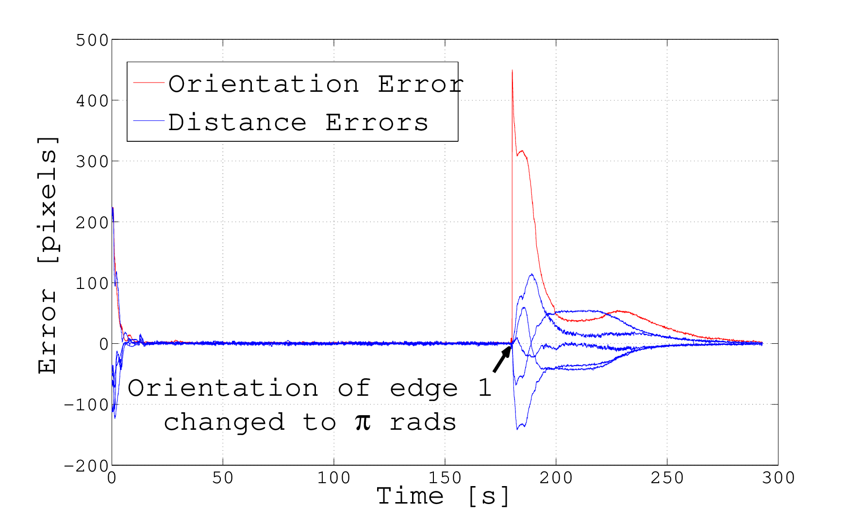
In this experiment we will validate the results from Theorem VI.2. We consider four robots that have a square with pixels (mm) for the length of the side as a prescribed shape . The incidence matrix describing the sensing topology for maintaining the prescribed shape and the derived are
We designate the robot number to be the agent that controls the orientation of , which is associated to the edge . We take for the potential function (3). We implement the control law (36) but noting that now is not constant and equal to the identity matrix anymore. The chosen speed for the translation is pixels/s (cm/s), and we set the desired heading of the translational motion to be the same as the one defined by the direction of . Because of simplicity and in order to show that Assumption VI.1 is only a sufficient condition, for achieving the mentioned desired steady-state velocity we set the motion parameters as
| (56) |
At the beginning of the experiment robot has for the desired orientation the vector pixels. Therefore the desired heading of the formation is radians with respect to . The robots start in random positions close to the origin of . During the experiment, once the agent reaches the imaginary vertical line crossing the position pixels, the value of changes to pixels. Therefore the formation will switch to a heading of radians with respect to . The gain in (36) has been set to . As a remark the chosen is smaller than the conservative in Theorem VI.2. The experimental results are discussed in Figure 5.
Remark VII.1
Since all the unicycle robots have the same reference point for the feedback linearization, once the system is at and , i.e. all the robots have the same velocity , the headings of the robots achieve consensus, i.e. all the robots are pointing at the same direction.
VII-B Enclosing and tracking a target experiment
We consider the scenario of having three pursuers and one independent target, set as agent , with constant velocity pixels/s. The velocity is unknown for the three pursuers. We ask the pursuers to form the shape in Figure 4 together with the target.
The incidence matrix corresponding to the sensing topology for the shape in Figure 4 and the derived matrix are
We ask the pursuers to maintain the following set of inter-agent distances
| (57) |
where pixels. We choose for the potential (3) and implement the controls (44) and (45) to the robots. Note that again since , we do not have being constant and equal to the identity anymore. The motion parameters for orbiting around the target are
| (58) |
where . Note that and are zero since they correspond to the target. The agents and are only using and respectively since and are perpendicular to . We set the desired steady-state angular speed to rads/s, therefore from (55) the value of is
We have set the control gains and to and respectively in (44) and (45). The gain has been chosen small in order to prevent saturation in the robots. The chosen is smaller than in , showing the conservative result of in Theorem VI.5. The initial values for of the estimators have been set to zero. The experimental results are discussed in Figure 6. Note that despiting of the local result in Theorem VI.5, the initial conditions and have been set relatively far away from the desired equilibrium.
VIII Conclusions
In this paper we have presented a distributed motion controller for rigid formations, which is compatible with the popular gradient-based controllers. The proposed controller allows us to design the steady-state formation motion in the desired shape with respect to a frame attached to the rigid formation. The steady-state velocity vector can be decomposed into two independent terms: one for the constant translation of the centroid of the formation and the other for a constant rotational formation motion around its centroid. Such design has been achieved by motion parameters in the prescribed distances between the agents. Two main applications based on the motion controller have been presented: the first is controlling the heading of a pure translational formation motion and the second is addressing the problem of enclosing and tracking a target. Experiments with mobile robots in have been presented in order to validate the proposed applications. We are currently working on extending the mathematical system model to accommodate agent dynamics modeled by double-integrators. We are also interested in testing our presented results in 3D scenarios involving flying drones.




References
- [1] Y. Lan, G. Yan, and Z. Lin, “Distributed control of cooperative target enclosing based on reachability and invariance analysis,” Systems and Control Letters, vol. 59, no. 7, pp. 381 – 389, 2010.
- [2] J. Yuan, Y. Huang, T. Tao, and F. Sun, “A cooperative approach for multi-robot area exploration,” in Proc. of IEEE International Conference on Intelligent Robots and Systems (IROS), 2010, pp. 1390–1395.
- [3] D. M. Stipanovic, C. R. Graunke, K. A. Intlekofer, and M. W. Spong, “Formation control and collision avoidance for multi-agent non-holonomic systems: Theory and experiments,” International Journal of Robotics Research, vol. 27, pp. 107–126, 2008.
- [4] E.Vos, J. Scherpen, and A. van der Schaft, “Port-hamiltonian approach to deployment,” in Proc. of International Symposium on Mathematical Theory of Networks and Systems, 2012.
- [5] H. Bai, M. Arcak, and J. Wen, Cooperative Control Design: A Systematic, Passivity-Based Approach. New York: Springer, 2011.
- [6] R. Skjetne, S. Moi, T. Fossen et al., “Nonlinear formation control of marine craft,” in Decision and Control, 2002, Proceedings of the 41st IEEE Conference on, vol. 2. IEEE, 2002, pp. 1699–1704.
- [7] G. Antonelli, F. Arrichiello, and S. Chiaverini, “Experiments of formation control with multirobot systems using the null-space-based behavioral control,” Control Systems Technology, IEEE Transactions on, vol. 17, no. 5, pp. 1173–1182, 2009.
- [8] R. Olfati-Saber and R. M. Murray, “Graph rigidity and distributed formation stabilization of multi-vehicle systems,” in Proc. of the 41st IEEE CDC, 2002, pp. 2965–2971.
- [9] L. Krick, M. E. Broucke, and B. A. Francis, “Stabilization of infinitesimally rigid formations of multi-robot networks,” International Journal of Control, vol. 82, pp. 423–439, 2009.
- [10] C. Yu, B. D. O. Anderson, S. Dasgupta, and B. Fidan, “Control of minimally persistent formations in the plane,” SIAM Journal on Control and Optimization, vol. 48, pp. 206–233, 2009.
- [11] M. Cao, C. Yu, and B. D. O. Anderson, “Formation control using range-only measurements,” Automatica, vol. 47, pp. 776–781, 2011.
- [12] A. Belabbas, S. Mou, A. Morse, and B. Anderson, “Robustness issues with undirected formations,” in Proc. of the 51st IEEE Conference on Decision and Control, Hawaii, USA, 2012, pp. 1445–1450.
- [13] S. Mou, A. S. Morse, A. Belabbas, Z. Sun, and B. Anderson, “Undirected rigid formations are problematic,” IEEE Transactions on Automatic Control., 2015.
- [14] U. Helmke, S. Mou, Z. Sun, and B. D. O. Anderson, “Geometrical methods for mismatched formation control,” in Proc. of the 53rd Conference on Decision and Control, 2014, pp. 1341–1346.
- [15] H. Garcia de Marina, M. Cao, and B. Jayawardhana, “Controlling rigid formations of mobile agents under inconsistent measurements,” Robotics, IEEE Transactions on, vol. 31, no. 1, pp. 31–39, Feb 2015.
- [16] Z. Sun, S. Mou, B. Anderson, and A. Morse, “Formation movements in minimally rigid formation control with mismatched mutual distances,” in Proc of the 53rd Conference on Decision and Control, 2014.
- [17] J. Guo, G. Yan, and Z. Lin, “Local control strategy for moving-target-enclosing under dynamically changing network topology,” Systems & Control Letters, vol. 59, no. 10, pp. 654 – 661, 2010.
- [18] A. Marasco, S. Givigi, and C. Rabbath, “Model predictive control for the dynamic encirclement of a target,” in American Control Conference (ACC), 2012, June 2012, pp. 2004–2009.
- [19] L. Asimow and B. Roth, “The rigidity of graphs, ii,” Journal of Mathematical Analysis and Applications, pp. 171–190, 1979.
- [20] B. D. O. Anderson, C. Yu, B. Fidan, and J. Hendrickx, “Rigid graph control architectures for autonomous formations,” IEEE Control Systems Magazine, vol. 28, pp. 48–63, 2008.
- [21] Henneberg, “Die graphische statik der starren systeme,” Leipzig, 1911.
- [22] P. Absil and K. Kurdyka, “On the stable equilibrium points of gradient systems,” Systems & Control Letters, pp. 573–577, 2006.
- [23] K. Oh and H. Ahn, “Distance-based undirected formation of single-integrator and double-integrator modeled agents in n-dimensional space,” International Journal of Robust and Nonlinear Control, pp. 1809–1820, 2014.
- [24] Y. Tian and Q. Wang, “Global stabilization of rigid formations in the plane,” Automatica, vol. 49, pp. 1436–1441, 2013.
- [25] H. Goldstein, Classical Mechanics. Addison-wesley, 1951.
- [26] N. Chopra, “Output synchronization on strongly connected graphs,” Automatic Control, IEEE Transactions on, vol. 57, no. 11, pp. 2896–2901, Nov 2012.
- [27] I. Shames, S. Dasgupta, B. Fidan, and B. Anderson, “Circumnavigation using distance measurements under slow drift,” Automatic Control, IEEE Transactions on, vol. 57, no. 4, pp. 889–903, April 2012.
- [28] F. Mondada, M. Bonani, X. Raemy et al., “The e-puck, a robot designed for education in engineering,” in Proc. of the 9th Conference on Autonomous Robot Systems and Competitions, 2009, pp. 59–65.
![[Uncaptioned image]](1604.07849v2/hector2.png) |
Hector G. de Marina received the M.Sc. degree in electronics engineering from Complutense University of Madrid, Madrid, Spain in 2008, the M.Sc. degree in control engineering from the University of Alcala de Henares, Alcala de Henares, Spain in 2011, and the Ph.D. degree in applied mathematics from the University of Groningen, the Netherlands. He is currently a postdoctoral researcher in the drones group at the School of Civil Aviation (ENAC), Toulouse, France. His research interests include formation control and navigation for autonomous robots. |
![[Uncaptioned image]](1604.07849v2/images/Bayu_Photo.jpg) |
Bayu Jayawardhana (SM’13) received the B.Sc. degree in electrical and electronics engineering from the Institut Teknologi Bandung, Bandung, Indonesia, in 2000, the M.Eng. degree in electrical and electronics engineering from the Nanyang Technological University, Singapore, in 2003, and the Ph.D. degree in electrical and electronics engineering from Imperial College London, London, U.K., in 2006. Currently, he is an associate professor in the Faculty of Mathematics and Natural Sciences, University of Groningen, Groningen, The Netherlands. He was with Bath University, Bath, U.K., and with Manchester Interdisciplinary Biocentre, University of Manchester, Manchester, U.K. His research interests are on the analysis of nonlinear systems, systems with hysteresis, mechatronics, systems and synthetic biology. He is a Subject Editor of the International Journal of Robust and Nonlinear Control, an associate editor of the European Journal of Control, and a member of the Conference Editorial Board of the IEEE Control Systems Society. |
![[Uncaptioned image]](1604.07849v2/images/web3.jpg) |
Ming Cao received the PhD degree in electrical engineering from Yale University, New Haven, CT, USA in 2007. He is an associate professor with tenure responsible for the research direction of network analysis and control at the University of Groningen, the Netherlands. His main research interest is in autonomous agents and multi-agent systems, mobile sensor networks and complex networks. He is an associate editor for IEEE Transactions on Circuits and Systems II, Systems and Control Letters, and for the Conference Editorial Board of the IEEE Control Systems Society. He is also a member of the IFAC Technical Committee on Networked Systems. |