Physical Layer Security in Millimeter Wave Cellular NetworksThanks: C. Wang and H.-M. Wang are with the School of Electronic and Information Engineering, and also with the MOE Key Lab for Intelligent Networks and Network Security, Xi’an Jiaotong University, Xi’an, 710049, Shaanxi, China. Email: wangchaoxuzhou@stu.xjtu.edu.cn and xjbswhm@gmail.com. The contact author is Hui-Ming Wang.

Chao Wang and Hui-Ming Wang Affiliation:

Abstract

Recent researches show that millimeter wave (mmWave) communications can offer orders of magnitude increases in the cellular capacity. However, the secrecy performance of a mmWave cellular network has not been investigated so far. Leveraging the new path-loss and blockage models for mmWave channels, which are significantly different from the conventional microwave channel, this paper comprehensively studies the network-wide physical layer security performance of the downlink transmission in a mmWave cellular network under a stochastic geometry framework. We first study the secure connectivity probability and the average number of perfect communication links per unit area in a noise-limited mmWave network for both non-colluding and colluding eavesdroppers scenarios, respectively. Then, we evaluate the effect of the artificial noise (AN) on the secrecy performance, and derive the analysis result of average number of perfect communication links per unit area in an interference-limited mmWave network. Numerical results are demonstrated to show the network-wide secrecy performance, and provide interesting insights into how the secrecy performance is influenced by various network parameters: antenna array pattern, base station (BS) intensity, and AN power allocation, etc.

Index Terms:

Millimeter wave network, physical layer security, stochastic geometry, Poisson point process, artificial noise

I Introduction

Within the next 20 years, wireless data traffic can be anticipated to skyrocket 10,000 folds, spurred by the popularity of various intelligent devices. Conventional communication means are difficult to meet such incredible increase in the wireless data traffic. Millimeter wave cellular communication has received an increasing attention due to the large available bandwidth at millimeter wave frequencies [1]. Recent field measurements have shown the huge advantages of mmWave networks, compared with the conventional microwave network in band below 6 GHz [1, 2, 3]. Due to the small wavelength, the mmWave cellular network is different from the conventional microwave network in the following ways: large number of antennas, sensitivity to blockages, and variable propagation laws, etc [4]. Recently, based on the real-world measurements in [3], spatial statistical models of the mmWave channel have been built in [5], which reveal the different path loss characteristics of the line-of-sight (LOS) and non-line-of-sight (NLOS) links. Under the new channel model, the network-wide performance of a mmWave cellular has attracted increasing attentions, and many works have investigated the SINR distribution, coverage, and average ergodic rate of the network under a stochastic geometry framework [6]-[11]. They show that the mmWave network has a great potential to provide tremendous data traffic increase.

All the above works have focused on the rate/reliability performance of the mmWave network, however, its secrecy performance has not been investigated so far. Given the ubiquitousness of wireless connections, an enormous amount of sensitive and confidential information, e.g. financial data, electronic cryptography, and private video, have been transmitted via wireless channels. Thus, providing a secure service is one of the top priorities in the design and implementation of mmWave networks [12]. In this paper, we investigate the physical layer security performance of mmWave networks by adopting the stochastic geometry framework.

I-A Background

Physical layer security has been identified as a promising strategy that exploits randomness of wireless medium to protect the confidential information from wiretapping [13], [14]. Recently, multiple-antenna technology becomes a powerful tool for enhancing the physical layer security in random networks [15]. With the degrees of freedom provided by multiple antennas, the transmitter can adjust its antenna steering orientation to exploit the maximum directivity gain while reducing the signal leakage to eavesdroppers [16]-[17], or radiate the artificial nosie (AN) for jamming potential eavesdroppers [18]-[19]. The secure connectivity, secrecy rate and secrecy outage with multi-antenna transmissions in wireless random networks have been studied in [16]-[17], respectively. The impact of AN on the security of random networks has been studied in [19].

However, all of the above works focus on conventional microwave networks, and the obtained results can not be applied to mmWave networks directly, due to the distinctive features of mmWave channel characteristics. For example, mmWave signals are more sensitive to blockage effects, and the fading statistical characteristics of the LOS link and NLOS link are totally different [3]. For characterizing the blockage effects of mmWave signals, different mmWave channel models have been proposed in [4]-[11]. In [6], an exponential blockage model has been proposed, and such model has been approximated as a LOS ball based blockage model for the coverage analysis in [4, 7]. In [8], the authors adopted the exponential blockage model to perform the coverage and capacity analysis for mmWave ad hoc networks. In [10], the authors proposed a ball based blockage model which is validated by using field measurements in New York and Chicago. Taking the outage state emerging in the mmWave communication into consideration, in [11], the authors have proposed a two-ball approximate blockage model for the analysis of the coverage and average rate of the multi-tier mmWave cellular network.

Under these new characteristics of mmWave channels, the secrecy performance of a mmWave cellular network will be significantly different from the conventional microwave network, which should be re-evaluated. The efficiency of traditional physical layer security techniques should be re-checked as well. Recently, the secrecy performance of a point-to-point mmWave communication has been studied in [25], which has shown that mmWave systems can enable significant secrecy improvement compared with conventional microwave systems. However, the network-wide secrecy performance of the mmWave cellular communication is still unknown, which motivates our work.

I-B Contribution

In this paper, using the stochastic geometry framework and the blockage model proposed in [10], we proposed a systematic secrecy performance analysis approach for the mmWave cellular communication, by modeling the random locations of the BSs and eavesdroppers as two independent homogeneous Possion point processes (PPPs). Our contributions can be summarized as follows:

1.

Secrecy performance analysis of noise-limited mmWave cellular networks. We characterize the secrecy performance of a noise-limited mmWave cellular network that is applicable to medium/sparse network deployments, where each BS only adopts the directional beamforming to transmit the confidential information. Considering two cases: the non-colluding eavesdropper case and the colluding eavesdroppers case, we derive the analysis result of the secure connectivity probability and the cumulative distribution function (CDF) of the received SNR at the typical receiver and eavesdropper, respectively. The secure connectivity probability facilitates the evaluation of the probability of the existence of secure connections from a typical transmitter to its intended receiver. With the CDF of the received SNR at the typical receiver and eavesdropper, we can characterize the average number of perfect communication links per unit area statistically in the random network. We show that the high gain narrow beam antenna is very important for enhancing the secrecy performance of mmWave networks.
2.

Secrecy performance analysis of AN assisted mmWave cellular networks. When AN is transmitted concurrently with the confidential information for interfering potential eavesdroppers, the AN radiation would increase the network interference. Thus, taking the network interference into consideration, we characterize the CDF of received SINRs at the intended receiver and non-colluding eavesdroppers. The secrecy probability and average number of perfect communication links per unit area for the AN assisted transmission have also been derived. The optimal power allocation between the AN and confidential signal is shown to depend on the array pattern and the intensity of eavesdroppers.

I-C Paper Organization and Notations

In Section II, the system model and mmWave channel characteristics are introduced. In Section III, considering the noise-limited mmWave cellular communication, we characterize the secure connectivity probability and average number of perfect communication links per unit area. In Section IV, taking the inter-cell interference into consideration, we characterize the average number of perfect communication links per unit area of the AN-assisted mmWave communication. Numerical results are provided in Section V and the paper is concluded in Section VI.

Notation: $x\sim\textrm{gamma}(k,m)$ denotes the gamma-distributed random variable with shape $k$ and scale $m$ , $\gamma(x,y)$ is the lower incomplete gamma function [30, 8.350.1], $\Gamma(x)$ is the gamma function [30, eq. (8.310)], and $\Gamma(a,x)$ is the upper incomplete function [30, 8.350.2]. $b(o,D)$ denotes the ball whose center is origin and radius is $D$ . The factorial of a non-negative integer $n$ is denoted by $n!$ , $\mathbf{x}\sim\mathcal{CN}\left(\mathbf{\Lambda},\mathbf{\Delta}\right)$ denotes the circular symmetric complex Gaussian vector with mean vector $\mathbf{\Lambda}$ and covariance matrix $\mathbf{\Delta}$ , $\binom{n}{k}=\frac{n!}{\left(n-k\right)!k!}$ . $\mathcal{L}_{X}(s)$ denotes the Laplace transform of $X$ , i.e., $\mathbb{E}\left(e^{-sX}\right)$ . ${}_{2}F_{1}(\alpha,\beta;\gamma,z)$ is the Gauss hypergeometric function [30, eq. (9.100)].

II System Model and Problem Formulation

We consider the downlink secure communication in the mmWave cellular network, where multiple spatially distributed BSs transmit the confidential information to authorized users in the presence of multiple malicious eavesdroppers. In the following subsections, we first introduce the system model and channel characteristics adopted in this paper, which have been validated in [4, 8, 10]. With such models, we give some important results on probability theory which will be used in the performance analysis. The secrecy performance metrics adopted are given in Section II-G.

II-A BS and eavesdropper layout

The locations of the BSs are modeled by a homogeneous PPP $\Phi_{B}$ of intensity $\lambda_{B}$ . Using PPP for modeling the irregular BSs locations has been shown to be an accurate and tractable approach for characterizing the downlink performance of the cellular network [28]. Just as [19]-[20], the locations of multiple eavesdroppers are modeled as an independent homogeneous PPP, $\Phi_{E}$ , of intensity $\lambda_{E}$ . Such random PPP model is well motivated by the random and unpredictable eavesdroppers’ locations. Furthermore, just as [19], [21]-[23], we consider the worst-case scenario by facilitating the eavesdroppers’ multi-user decodability, i.e., eavesdroppers can perform successive interference cancellation [24] to eliminate the interference due to the information signals from other interfering BSs. The total transmit power of each BS is $P_{t}$ .

II-B Directional beamforming

For compensating the significant path-loss at mmWave frequencies, highly directional beamforming antenna arrays are deployed at BSs to perform the directional beamforming. For mathematical tractability and similar to [4, 8, 10, 11], the antenna pattern is approximated by a sectored antenna model in [26]. In particular,

\displaystyle G_{b}(\theta)=\left\{\begin{array}[]{ll}M_{s},&\mathrm{if}\quad|\theta|\leq\theta_{b}\\ m_{s},&\textrm{Otherwise},\end{array}\right.

where $\theta_{b}$ is the beam width of the main lobe, $M_{s}$ and $m_{s}$ are the array gains of main and sidelobes, respectively. In this paper, we assume that each BS can get the perfect CSI estimation, including angles of arrivals and fading, and then, they can adjust their antenna steering orientation array for adjusting the boresight direction of antennas to their intended receivers and maximizing the directivity gains. In the following, we denote the boresight direction of the antennas as $0^{o}$ . Therefore, the directivity gain for the intended link is $M_{s}$ . For each interfering link, the angle $\theta$ is independently and uniformly distributed in $\left[-\pi,\pi\right]$ , which results in a random directivity gain $G_{b}(\theta)$ . For simplifying the performance analysis, just as [10, 25], the authorized users and malicious eavesdroppers are both assumed to be equipped with a single omnidirectional antenna in this paper. ¹¹ 1 This assumption is just for simplifying the performance analysis. However, the obtained analysis methods can be extended to the multiple antennas case directly by modeling the array pattern at authorized users and malicious eavesdroppers in a similar way as (II-B).

II-C Small-scale fading

Just as [4, 8], we assume that the small-scale fading of each link follows independent Nakagami fading, and the Nakagami fading parameter of the LOS (NLOS) link is $N_{L}$ ( $N_{N}$ ). For simplicity, $N_{L}$ and $N_{N}$ are both assumed to be positive integers. In the following, the small-scale channel gain from the BS at $x\in\mathbb{R}^{2}$ to the authorized user (eavesdropper) at $y\in\mathbb{R}^{2}$ is expressed as $h_{xy}$ ( $g_{xy}$ ).

II-D Blockage Model

The blockage model proposed in [10] is adopted, which can be regarded as an approximation of the statistical blockage model in [5, eq. (8)], [11], and incorporates the LOS ball model proposed in [4, 7] as a special case. As shown by [9, 10], the blockage model proposed in [10] is simple yet flexible enough to capture blockage statistics, coverage and rate trends in mmWave cellular networks. In particular, defining $q_{L}(r)$ as the probability that a link of length $r$ is LOS,

\displaystyle q_{L}(r)=\left\{\begin{array}[]{ll}C,&\mathrm{if}\quad r\leq D,\\ 0,&\textrm{Otherwise},\end{array}\right.

for some $0\leq C\leq 1$ . The parameter $C$ can be interpreted as the average LOS area in the spherical region around a typical user. The empirical $(C,D)$ for Chicago and Manhattan are $(0.081,250)$ and $(0.117,200)$ , respectively [10], which would be adopted in the simulation results. With such blockage model, the BS process in $b(o,D)$ can be divided into two independent PPPs: the LOS BS process $\Phi_{L}$ with intensity $C\lambda_{B}$ and NLOS BS process with intensity $(1-C)\lambda_{B}$ [28, Proposition 1.3.5]. Outside $b(o,D)$ , only the NLOS BS process exists with intensity $\lambda_{B}$ . We denote the whole NLOS BS process as $\Phi_{N}$ .

II-E Path loss model

Just as [4, 10], different path loss laws are applied to LOS and NLOS links. In particular, given a link from $x\in\mathbb{R}^{2}$ to $y\in\mathbb{R}^{2}$ , its path loss $L(x,y)$ can be calculated by

\displaystyle L(x,y)=\left\{\begin{array}[]{ll}C_{L}||x-y||^{-\alpha_{L}},&\textrm{ if link }x\rightarrow y\textrm{ is LOS link},\\ C_{N}||x-y||^{-\alpha_{N}},&\textrm{ if link }x\rightarrow y\textrm{ is NLOS link},\end{array}\right.

where $\alpha_{L}$ and $\alpha_{N}$ are the LOS and NLOS path loss exponents, and $C_{L}\triangleq 10^{-\frac{\beta_{L}}{10}}$ and $C_{N}\triangleq 10^{-\frac{\beta_{N}}{10}}$ can be regarded as the path-loss intercepts of LOS and NLOS links at the reference distance. Typical $\alpha_{j}$ and $\beta_{j}$ for $j\in\{L,N\}$ are defined in [5, Table I]. For exmple, for 28 GHz bands, $\beta_{L}=61.4$ , $\alpha_{L}=2,$ and $\beta_{N}=72$ , $\alpha_{N}=2.92$ . From the measured values of $C_{j}$ and $\alpha_{j},$ $j\in\{L,N\}$ in [5, Table I], we know that it satisfies $C_{L}>C_{N}$ and $\alpha_{L}<\alpha_{N}$ .

II-F User association

For maximizing the receiving quality of authorized users [4, 10], one authorized user is assumed to be associated with the BS offering the lowest path loss to him, since the network considered is homogeneous. Thus, for the typical authorized user at origin, its serving BS is located at $x^{*}\triangleq\arg\max_{x\in\Phi_{B}}L(x,o)$ . Denoting the distance from the typical authorized user to the nearest BS in $\Phi_{j}$ as $d^{*}_{j}$ for $j=\{L,N\}$ , the following Lemma 1 provides their probability distribution functions (pdf), and the obtained statistics hold for a generic authorized user, due to Slivnyak’s theorem [28].

Lemma 1

Given the typical authorized user observes at least one LOS BS, the pdf of $d^{*}_{L}$ is

\displaystyle f_{d^{*}_{L}}(r)=\frac{2\pi C\lambda_{B}r\textrm{exp}(-\pi C\lambda_{B}r^{2})}{1-\textrm{exp}(-\pi C\lambda_{B}D^{2})},\textrm{ for }r\in\left[0,D\right].

(7)

On the other hand, the pdf of $d^{*}_{N}$ is given by

\displaystyle f_{d^{*}_{N}}(r)=2\pi(1-C)\lambda_{B}re^{-\pi(1-C)\lambda_{B}r^{2}}\mathbb{I}\left(r\leq D\right)+2\lambda_{B}\pi re^{-\lambda_{B}\pi\left(r^{2}-D^{2}\right)}e^{-\pi(1-C)\lambda_{B}D^{2}}\mathbb{I}\left(r>D\right),

(8)

where $\mathbb{I}\left(.\right)$ is the indicator function.

Proof:

The proof is given in Appendix A. ∎Then, the following lemma gives the probability that the typical authorized user is associated with a LOS or NLOS BS.

Lemma 2

The probability that the authorized user is associated with a NLOS BS, $A_{N}$ , is given by

\displaystyle A_{N}=

\displaystyle\int^{\mu}_{0}{\left(\textrm{e}^{-\pi C\lambda_{B}\left(\frac{C_{L}}{C_{N}}\right)^{\frac{2}{\alpha_{L}}}x^{\frac{2\alpha_{N}}{\alpha_{L}}}}-\textrm{e}^{-\pi C\lambda_{B}D^{2}}\right)2\pi(1-C)\lambda_{B}x}\textrm{e}^{-\pi(1-C)\lambda_{B}x^{2}}dx+\textrm{e}^{-\pi C\lambda_{B}D^{2}},

(9)

where $\mu\triangleq\left(\frac{C_{L}}{C_{N}}\right)^{-\frac{1}{\alpha_{N}}}D^{\frac{\alpha_{L}}{\alpha_{N}}}$ . The probability that the typical authorized user is associated with a LOS BS is given by $A_{L}=1-A_{N}$ .

Proof:

The proof is given in Appendix B. ∎

With the smallest path loss association rule, the typical authorized user would be associated with the nearest LOS BS in $\Phi_{L}$ or the nearest NLOS BS in $\Phi_{N}$ . The following lemma gives the pdf of the distance between the typical authorized user and its serving BS in $\Phi_{j}$ , i.e., $r_{j}$ , $\forall j\in\{L,N\}$ .

Lemma 3

On the condition that the serving BS is in $\Phi_{L}$ , the pdf of the distance from the typical authorized user to its serving BS in $\Phi_{L}$ is

\displaystyle f_{r_{L}}(r)=\frac{\textrm{exp}\left(-(1-C)\lambda_{B}\pi\left(\frac{C_{N}}{C_{L}}\right)^{\frac{2}{\alpha_{N}}}r^{\frac{2\alpha_{L}}{\alpha_{N}}}\right)2\pi C\lambda_{B}r\textrm{exp}\left(-C\lambda_{B}\pi r^{2}\right)}{A_{L}}\textrm{, }r\in\left[0,D\right].

(10)

On the condition that the serving BS is in $\Phi_{N}$ , the pdf of the distance from the typical authorized user to its serving BS in $\Phi_{N}$ is

		$\displaystyle f_{r_{N}}(r)=\frac{2\pi\lambda_{B}r\textrm{exp}\left(-\pi\lambda_{B}r^{2}\right)\left(\left(1-C\right)\textrm{exp}\left(\pi C\lambda_{B}\left(r^{2}-D^{2}\right)\right)\mathbb{I}\left(r\leq D\right)+{\mathbb{I}\left(r\geq D\right)}\right)}{A_{N}}$
		$\displaystyle+\frac{2\pi(1-C)\lambda_{B}re^{-(1-C)\lambda_{B}\pi r^{2}}\left(e^{-C\lambda_{B}\pi\left(\frac{C_{L}}{C_{N}}\right)^{\frac{2}{\alpha_{L}}}r^{\frac{2\alpha_{N}}{\alpha_{L}}}}-e^{-C\lambda_{B}\pi D^{2}}\right)}{A_{N}}\mathbb{I}\left(r\leq\left(\frac{C_{N}}{C_{L}}\right)^{\frac{1}{\alpha_{N}}}D^{\frac{\alpha_{L}}{\alpha_{N}}}\right).$		(11)

Proof:

The proof is given in Appendix C. ∎

II-G Secrecy Performance Metric

In this paper, we assume that the channels are all quasi-static fading channels. The legitimate receivers and eavesdroppers can obtain their own CSI, but mmWave BSs do not know the instantaneous CSI of eavesdroppers. For protecting the confidential information from wiretapping, each BS encodes the confidential data by the Wyner code [13]. Then two code rates namely, the rate of the transmitted codewords $R_{b}$ , and the rate of the confidential information $R_{s}$ should be determined before the data transmission, and $R_{b}-R_{s}$ is the cost for securing the confidential information. The details of the code construction can be found in [13, 27]. In this paper, just as [19, 20, 27], we adopt the fixed rate transmission, where $R_{b}$ and $R_{s}$ are fixed during the information transmission. For the secrecy transmission over quasi-static fading channels, the perfect secrecy can not always be guaranteed. Therefore, as indicated in [16, 20, 27], an outage-based secrecy performance metric is more suitable. Therefore, we analyze the secrecy performance of the mmWave communication by considering both the secure connectivity probability and average number of perfect communication links per unit area.

1.

Secure connectivity probability [16]. Secure connectivity probability introduced in [16], is defined as the probability that the secrecy rate is nonnegative. Using the secure connectivity probability, we aim to statistically characterize the existence of secure connection between any randomly chosen BS and its intended authorized user in the presence of multiple eavesdroppers.
2.
Average number of perfect communication links per unit area [20].When $R_{b}$ and $R_{s}$ are given, we define the links that have perfect connection and secrecy as perfect communication links. Then, the mathematical definition of the average number of perfect communication links per unit area is given as follows.
- •
  
  Connection Probability. When $R_{b}$ is below the capacity of legitimate links, authorized users can decode signals with an arbitrary small error, and thus perfect connection can be assured. Otherwise, connection outage would occur. The connection probability is denoted as $p_{con}$ .
- •
  
  Secrecy Probability. When the wiretapping capacity of eavesdroppers is below the rate redundancy $R_{e}\triangleq R_{b}-R_{s}$ , there will be no information leakage to potential eavesdroppers, and thus perfect secrecy of the link can be assured [13]. Otherwise, secrecy outage would occur. The secrecy probability is denoted as $p_{sec}$ .
Following [20, eq. (29)], the average number of perfect communication links per unit area is

$\displaystyle N_{p}=\lambda_{B}p_{con}p_{sec}.$ (12)

Remark 1

With the given $R_{b}$ and $R_{s}$ , the average achievable secrecy throughput per unit area $\omega$ can be calculated by $\omega=N_{p}R_{s}.$

III Secrecy Performance of the Noise-Limited Millimeter Wave Communication

In this section, we evaluate the secrecy performance of the direct transmission for the noise-limited mmWave communication. As pointed out by [3, 5, 10, 11], highly directional transmissions used in mmWave systems combined with short cell radius results in links that are noise-dominated, especially for densely blocked settings (e.g., urban settings) and medium/sparse network deployments [10, 11]. This distinguishes from current dense cellular deployments where links are overwhelmingly interference-dominated. Therefore, just as [10, 11], we first study the secrecy performance of the noise-limited mmWave communication without considering the effect of inter-cell interference. The received SNR by the typical authorized user at origin and the eavesdropper at $z$ with respect to the serving BS can be expressed as $\textrm{SNR}_{U}=\frac{P_{t}M_{s}L(x^{*},o)h_{x^{*}o}}{N_{0}}$ and $\textrm{SNR}_{E_{z}}=\frac{P_{t}G_{b}(\theta)L(x^{*},z)g_{x^{*}z}}{N_{0}}$ . $N_{0}$ is the noise power in the form of $N_{0}=10^{\frac{N_{0}(dB)}{10}}$ , where $N_{0}(dB)=-174+10\textrm{log}_{10}(\textrm{BW})+\mathcal{F}_{dB}$ , BW is the transmission bandwidth and $\mathcal{F}_{dB}$ is the noise figure [11]. With the array pattern in (II-B), $G_{b}(\theta)$ seen by the eavesdropper is a Bernoulli random variable whose probability mass function (PMF) is given by

\displaystyle G_{b}(\theta)=\left\{\begin{matrix}M_{s},&\textrm{Pr}_{G_{b}}(M_{s})\triangleq\textrm{Pr}\left(G_{b}(\theta)=M_{s}\right)=\frac{\theta_{b}}{180},\\ m_{s},&\ \ \textrm{Pr}_{G_{b}}(m_{s})\triangleq\textrm{Pr}\left(G_{b}(\theta)=m_{s}\right)=\frac{180-\theta_{b}}{180}.\end{matrix}\right.

(13)

III-A Non-colluding Eavesdroppers

In this subsection, assuming that the random distributed eavesdroppers are non-colluding, we evaluate the secrecy performance of the mmWave cellular network.

III-A1 Secure Connectivity Probability

We first study the secure connectivity probability, $\tau_{n}$ , of the mmWave communication in the presence of multiple non-colluding eavesdroppers. A secure connection is possible if the condition $\frac{M_{s}L(x^{*},o)h_{x^{*}o}}{\max_{z\in\Phi_{E}}G_{b}(\theta)L(x^{*},z)g_{x^{*}z}}\geq 1$ holds [16], and the secure connectivity probability can be calculated by $\tau_{n}=\textrm{Pr}\left(\frac{M_{s}L(x^{*},o)h_{x^{*}o}}{\max_{z\in\Phi_{E}}G_{b}(\theta)L(x^{*},z)g_{x^{*}z}}\geq 1\right)$ . We can see that the wiretapping capability of multiple eavesdroppers is determined by the path loss process $G_{b}(\theta)L(x^{*},z)g_{x^{*}z}$ . Thus, for facilitating the performance evaluation, the following process is introduced.

Definition 1

The path loss process with fading (PLPF), denoted as $\mathcal{N}_{E}$ , is the point process on $\mathbb{R}^{+}$ mapped from $\Phi_{E}$ , where $\mathcal{N}_{E}\triangleq\left\{\varsigma_{z}=\frac{1}{G_{b}(\theta)g_{xz}L(x,z)},z\in\Phi_{E}\right\}$ and $x$ denotes the location of the wiretapped BS. We sort the elements of $\mathcal{N}_{E}$ in ascending order and denote the sorted elements of $\mathcal{N}_{E}$ as $\left\{\xi_{i},i=1,\ldots\right\}$ . The index is introduced such that $\xi_{i}\leq\xi_{j}$ for $\forall i<j$ .

Note that $\mathcal{N}_{E}$ involves both the impact of small fading and spatial distribution of eavesdroppers, which is an ordered process. Consequently, $\mathcal{N}_{E}$ determines the wiretapping capability of eavesdropper. We then have the following lemma.

Lemma 4

The PLPF $\mathcal{N}_{E}$ is an one-dimensional nonhomogeneous PPP with the intensity measure

\displaystyle\Lambda_{E}\left(0,t\right)=

\displaystyle 2\pi\lambda_{E}\left(\sum_{j\in\left\{L,N\right\}}q_{j}\left(\Omega_{j,\textrm{in}}\left(M_{s},t\right)+\Omega_{j,\textrm{in}}\left(m_{s},t\right)\right)+\Omega_{N,\textrm{out}}\left(M_{s},,t\right)+\Omega_{N,\textrm{out}}\left(m_{s},t\right)\right),

(14)

where $q_{L}\triangleq C$ , $q_{N}\triangleq 1-C$ , and $\Omega_{j,\textrm{in}}(V,t)\triangleq\textrm{Pr}_{G_{b}}(V)\frac{\left(VC_{j}t\right)^{\frac{2}{\alpha_{j}}}}{\alpha_{j}}\sum^{N_{j}-1}_{m=0}\frac{\gamma\left(m+\frac{2}{\alpha_{j}},\frac{D^{\alpha_{j}}}{VC_{j}t}\right)}{m!}$ , $\Omega_{j,\textrm{out}}(V,t)\triangleq\textrm{Pr}_{G_{b}}(V)\frac{\left(VC_{j}t\right)^{\frac{2}{\alpha_{j}}}}{\alpha_{j}}\sum^{N_{j}-1}_{m=0}\frac{\Gamma\left(m+\frac{2}{\alpha_{j}},\frac{D^{\alpha_{j}}}{VC_{j}t}\right)}{m!}$ , with $V\in\left\{M_{s},m_{s}\right\}$ .

Proof:

The proof is given in Appendix D. ∎

The following theorem gives the analysis result of the secure connectivity probability in the presence of non-colluding eavesdroppers.

Theorem 1

In the case of non-colluding eavesdroppers, the secure connectivity probability is

\displaystyle\tau_{n}=\sum_{j\in\{L,N\}}A_{j}\int^{D}_{0}f_{r_{j}}(r)dr\int^{+\infty}_{0}\frac{\textrm{e}^{-\Lambda_{E}\left(0,\frac{r^{\alpha_{j}}}{M_{s}wC_{j}}\right)}w^{N_{j}-1}e^{-w}}{\Gamma(N_{j})}dw.

(15)

Proof:

We have the following derivations:

Pr	$\displaystyle\left(\frac{M_{s}L(x^{},o)h_{x^{}o}}{\max_{z\in\Phi_{E}}G_{b}(\theta)L(x^{},z)g_{x^{}z}}\geq 1\right)=\textrm{Pr}\left(\min_{z\in\Phi_{E}}\frac{1}{G_{b}(\theta)L(x^{},z)g_{x^{}z}}\geq\frac{1}{M_{s}L(x^{},o)h_{x^{}o}}\right)$
	$\displaystyle\overset{(e)}{=}\textrm{Pr}\left(\xi_{1}\geq\frac{1}{M_{s}L(x^{},o)h_{x^{}o}}\right)\overset{(f)}{=}\mathbb{E}_{L(x^{},o),h_{x^{}o}}\left(\textrm{exp}\left(-\Lambda_{E}\left(0,\frac{1}{M_{s}L(x^{},o)h_{x^{}o}}\right)\right)\right)$
	$\displaystyle\overset{(g)}{=}A_{L}\mathbb{E}_{r_{L},h_{x^{}o}}\left(\textrm{exp}\left(-\Lambda_{E}\left(0,\frac{r_{L}^{\alpha_{L}}}{M_{s}C_{L}h_{x^{}o}}\right)\|\textrm{Serving BS is a LOS BS}\right)\right)+$
	$\displaystyle\qquad A_{N}\mathbb{E}_{r_{N},h_{x^{}o}}\left(\textrm{exp}\left(-\Lambda_{E}\left(0,\frac{r_{N}^{\alpha_{N}}}{M_{s}C_{N}h_{x^{}o}}\right)\|\textrm{Serving BS is a NLOS BS}\right)\right),$	(16)

where step $(e)$ is due to Definition 1, step $(f)$ follows the PPP’s void probability [28], and step ( $g$ ) is due to the law of total probability. When the serving BS is a LOS BS, $h_{x^{*}o}\sim\textrm{gamma}\left(N_{L},1\right)$ and the pdf of $r_{L}$ is given by (10), and when the serving BS is a NLOS BS, $h_{x^{*}o}\sim\textrm{gamma}\left(N_{N},1\right)$ and the pdf of $r_{N}$ is given by (11). Finally, substituting the pdf of $h_{x^{*}o}$ , $r_{L}$ , and $r_{N}$ into (16), $\tau_{n}$ can be obtained. ∎

Refer to caption — Fig. 1: Secure connectivity probability of the mmWave communication in the presence of multiple non-colluding eavesdroppers vs $\lambda_{E}$ with BW=2GHz, $P_{t}=30$ dB, $\mathcal{F}_{dB}=10$ , $\theta_{b}=9^{o}$ , $M_{s}=15$ dB, and $m_{s}=-3$ dB.

Theoretical results in Theorem 1 are validated in Fig. 1, where we plot the secure connectivity probability $\tau_{n}$ versus $\lambda_{E}$ . For all the simulations in this paper, 100000 trials are used. From Fig. 1, we can find that theoretical curves coincide with the simulation ones well, which validates the theoretical result in Theorem 1.

III-A2 Average number of perfect communication links per unit area

In the following, we study the average number of perfect communication links per unit area, $N_{p}$ , of the mmWave communication in the presence of non-colluding eavesdroppers. Firstly, we should derive the analytical result of the connection probability and secrecy probability of a mmWave communication link, given by

\displaystyle p_{con}\triangleq\textrm{Pr}\left(\textrm{SNR}_{U}\geq T_{c}\right)\textrm{ and }p_{sec,n}\triangleq\textrm{Pr}\left(\max_{z\in\Phi_{E}}\textrm{SNR}_{E_{z}}\leq T_{e}\right),

(17)

respectively, where $T_{c}\triangleq 2^{R_{c}-1}$ and $T_{e}\triangleq 2^{R_{e}-1}$ . We have the following theorem.

Theorem 2

For the non-colluding eavesdroppers case, the analytical result of $p_{con}$ is given by

\displaystyle p_{con}=\int^{D}_{0}\frac{\Gamma\left(N_{L},\frac{N_{0}T_{c}r^{\alpha_{L}}}{P_{t}M_{S}C_{L}}\right)}{\Gamma(N_{L})}f_{r_{L}}(r)drA_{L}+\int^{+\infty}_{0}\frac{\Gamma\left(N_{N},\frac{N_{0}T_{c}r^{\alpha_{N}}}{P_{t}M_{S}C_{N}}\right)}{\Gamma(N_{N})}f_{r_{N}}(r)drA_{N},

(18)

and the analytical result of $p_{sec,n}$ is given by

\displaystyle p_{sec,n}=\textrm{exp}\left(-\Lambda_{E}\left(0,\frac{1}{TeN_{0}}\right)\right).

(19)

Proof:

$p_{con}$ can be derived as follows

$\displaystyle p_{con}=$	$\displaystyle\textrm{Pr}\left(h_{x^{}o}\geq\frac{N_{0}T_{c}}{P_{t}M_{S}L(x^{},o)}\|\textrm{Serving BS is a LOS BS}\right)A_{L}+$
	$\displaystyle\textrm{Pr}\left(h_{x^{}o}\geq\frac{N_{0}T_{c}}{P_{t}M_{S}L(x^{},o)}\|\textrm{Serving BS is a NLOS BS}\right)A_{N}$
$\displaystyle=$	$\displaystyle\int^{D}_{0}\frac{\Gamma\left(N_{L},\frac{N_{0}T_{c}r^{\alpha_{L}}}{P_{t}M_{S}C_{L}}\right)}{\Gamma(N_{L})}f_{r_{L}}(r)drA_{L}+\int^{+\infty}_{0}\frac{\Gamma\left(N_{N},\frac{N_{0}T_{c}r^{\alpha_{N}}}{P_{t}M_{S}C_{N}}\right)}{\Gamma(N_{N})}f_{r_{N}}(r)drA_{N}.$	(20)

$p_{sec,n}$ can be derived as follows

\displaystyle p_{sec,n}

\displaystyle=\textrm{Pr}\left\{\frac{\max_{z\phi_{E_{z}}}G_{b}(\theta)L(x^{*},z)g_{x^{*},z}}{N_{0}}\leq T_{e}\right\}\overset{(g)}{=}\textrm{Pr}\left\{\frac{1}{\xi_{1}N_{0}}\leq T_{e}\right\}\overset{(h)}{=}\textrm{exp}\left(-\Lambda_{E}\left(0,\frac{1}{T_{e}N_{0}}\right)\right),

(21)

where step $(g)$ is due to Definition 1, and step $(h)$ is due to the PPP’s void probability [28]. ∎

III-B Colluding Eavesdroppers

In this subsection, we study the secrecy performance of the mmWave communication by considering the worst case: colluding eavesdroppers, where distributed eavesdroppers adopt the maximal-ratio combining to process the wiretapped confidential information.

III-B1 Secure Connectivity Probability

The secure connectivity probability $\tau_{c}$ in the presence of multiple colluding eavesdroppers can be calculated by

\displaystyle\tau_{c}=\textrm{Pr}\left(\frac{M_{s}L(x^{*},o)h_{x^{*}o}}{I_{E}}\geq 1\right),

(22)

where $I_{E}\triangleq{\sum_{z\in\Phi_{E}}G_{b}(\theta)L(x^{*},z)g_{x^{*}z}}$ . We have the following theorem.

Theorem 3

In the case of colluding eavesdroppers, $\tau_{c}$ can be calculated by

\displaystyle\tau_{c}=\mathbb{E}_{r_{j}}\left[\sum_{j\in\{L,N\}}\sum^{N_{j}-1}_{m=0}\left(\frac{r_{j}^{\alpha_{j}}}{M_{S}C_{j}}\right)^{m}\frac{A_{j}}{\Gamma(m+1)}(-1)^{m}\mathcal{L}^{(m)}_{I_{E}}\left(\frac{r_{j}^{\alpha_{j}}}{M_{S}C_{j}}\right)\right],

(23)

where $\mathcal{L}_{I_{E}}(s)\triangleq\textrm{exp}\left(\Xi(s)\right)$ and

$\displaystyle\Xi(s)\triangleq$	$\displaystyle-s\left(2\pi\lambda_{E}\sum_{j\in\{L,N\}}q_{j}\left(\sum_{V\in\{M_{s},m_{s}\}}\textrm{Pr}_{G_{b}}(V)\frac{\left(VC_{j}\right)^{\frac{2}{\alpha_{j}}}}{\alpha_{j}}\sum^{N_{j}-1}_{m=0}\frac{\left(D^{\alpha_{j}}/(VC_{j})\right)^{m+\frac{2}{\alpha_{j}}}}{\left(m+\frac{2}{\alpha_{j}}\right)\left(s+{D^{\alpha_{j}}/(VC_{j})}\right)^{m+1}}\right.\right.$
	$\displaystyle\left.{{}_{2}}F_{1}\left(1,m+1;m+\frac{2}{\alpha_{j}}+1;\frac{{D^{\alpha_{j}}/(VC_{j})}}{{D^{\alpha_{j}}/(VC_{j})}+s}\right)\Bigg)+2\pi\lambda_{E}\sum_{V\in\{M_{s},m_{s}\}}\textrm{Pr}_{G_{b}}(V)\frac{\left(VC_{N}\right)^{\frac{2}{\alpha_{N}}}}{\alpha_{N}}\right.$
	$\displaystyle\left.\sum^{N_{N}-1}_{m=0}\frac{\left(D^{\alpha_{N}}/(VC_{N})\right)^{m+\frac{2}{\alpha_{N}}}}{\left(1-\frac{2}{\alpha_{N}}\right)\left(s+D^{\alpha_{N}}/(VC_{N})\right)^{m+1}}{{}_{2}}F_{1}\left(1,m+1;2-\frac{2}{\alpha_{N}};\frac{s}{s+D^{\alpha_{N}}/(VC_{N})}\right)\right).$	(24)

Proof:

The proof is given in Appendix E. ∎

Although the analytical result given in Theorem 3 is general and exact, it is rather unwieldy, motivating the interest in acquiring a more compact expression. Exploring the tight lower bound of the CDF of the gamma random variable in [31], a tight upper bound of $\tau_{c}$ can be calculated as follows.

Theorem 4

$\tau_{c}$ can be tightly upper bounded by

\displaystyle\tau_{c}\lessapprox\sum_{j\in\{L,N\}}\sum^{N_{j}}_{n=1}\binom{N_{j}}{n}(-1)^{n+1}\int^{+\infty}_{0}f_{r_{j}}(r)\mathcal{L}_{I_{E}}\left(\frac{a_{j}nr^{\alpha_{j}}}{M_{S}C_{j}}\right)dr,

(25)

where $a_{L}\triangleq(N_{L})^{-\frac{1}{N_{L}}}$ and $a_{N}\triangleq(N_{N})^{-\frac{1}{N_{N}}}$ .

Proof:

We leverage the tight lower bound of the CDF of a normalized gamma random variable, $g$ with $N$ degrees of freedom as $\textrm{Pr}\left(x\leq y\right)\gtrapprox\left(1-e^{-\kappa y}\right)^{N}$ [31], where $\kappa=\left(N!\right)^{-\frac{1}{N}}$ . Since $h_{x^{*},o}$ is a normalized gamma random variable, we have

\displaystyle\tau_{c}\lessapprox 1-\sum_{j\in\{L,N\}}\mathbb{E}_{I_{E},r_{j}}\left(\left(1-\textrm{exp}\left(-\frac{na_{j}I_{E}r_{j}^{\alpha_{j}}}{M_{S}C_{j}}\right)\right)^{N_{j}}\right).

(26)

Using the binomial expansion, we can obtain

	$\displaystyle\tau_{c}$	$\displaystyle\lessapprox\sum_{j\in\{L,N\}}\sum^{N_{j}}_{n=1}\binom{N_{j}}{n}(-1)^{n+1}\mathbb{E}_{r_{j}}\left(\mathbb{E}_{I_{E}}\left(\textrm{exp}\left(-\frac{a_{j}nr_{j}^{\alpha_{j}}I_{E}}{M_{S}C_{j}}\right)\right)\right)$
		$\displaystyle=\sum_{j\in\{L,N\}}\sum^{N_{j}}_{n=1}\binom{N_{j}}{n}(-1)^{n+1}\int^{+\infty}_{0}f_{r_{j}}(r)\mathcal{L}_{I_{E}}\left(\frac{a_{j}nr^{\alpha_{j}}}{M_{S}C_{j}}\right).$		(27)

∎

The bounds in Theorem 4 are validated in Fig. 2, where we plot the secure connectivity probability $\tau_{c}$ versus $\lambda_{E}$ . From Fig. 2, we can find that theoretical curves coincide with simulation ones well, which show that the upper bound given in Theorem 4 is tight.

III-B2 Average number of perfect communication links per unit area

In the case of colluding eavesdroppers, the connection probability $p_{con}$ of the typical authorized user can be still calculated by (18) in Theorem 2, and the achievable secrecy probability $p_{sec}$ can be calculated by

\displaystyle p_{sec,c}=\textrm{Pr}\left\{\frac{P_{t}I_{E}}{N_{0}}\leq T_{e}\right\}.

(28)

For getting the analysis result of $p_{sec,c}$ in (28), the CDF of $I_{E}$ should be available. Although the CDF of $I_{E}$ can be obtained from its Laplace transform $\mathcal{L}_{I_{E}}(s)$ by using the inverse Laplace transform calculation [32], it could get computationally intensive in certain cases and may render the analysis intractable. As an alternative, we resort to an approximation method widely adopted in [4, 8, 10] for getting an approximation of $p_{sec,c}$ which is given in the following theorem.

Theorem 5

In the case of multiple colluding eavesdroppers, the approximation of $p_{sec,c}$ is given by

\displaystyle p_{sec,c}\lessapprox\sum^{N}_{n=1}\left(-1\right)^{n+1}\mathcal{L}_{I_{E}}\left(-\frac{an}{n_{0}T_{e}}\right),

(29)

where $\mathcal{L}_{I_{E}}(s)$ is given in Theorem 3, $a\triangleq(N!)^{\frac{1}{N}}$ and $N$ is the number of terms used in approximation.

Proof:

\displaystyle p_{sec,c}=\textrm{Pr}\left\{\frac{P_{t}I_{E}}{N_{0}T_{e}}\leq 1\right\}\overset{(i)}{\approx}\textrm{Pr}\left\{\frac{P_{t}I_{E}}{N_{0}T_{e}}\leq w\right\}.

(30)

In $(i)$ , $w$ is a normalized gamma random variable with a shape parameter, $N$ , and the approximation in $(i)$ is due to the fact that a normalized gamma random variable converges to identity when its shape parameter goes to infinity [4, 8].

Then, using the tight lower of the CDF of a normalized gamma random variable in [31], $p_{sec}$ can be tightly upper bounded by

\displaystyle p_{sec,c}\lessapprox 1-\left(1-\textrm{exp}\left(-\frac{aP_{t}I_{E}}{N_{0}T_{e}}\right)\right)^{N}.

(31)

Finally, using the binomial expansion, (31) can be further rewritten as (29). ∎

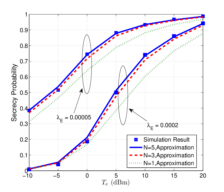
The approximate analysis result in Theorem 5 is validated in Fig. 3. From Fig. 3, we can find that when $N=5,$ (29) can give an accurate approximation. Then, in the following simulations, we set $N=5$ to calculate $p_{sec,c}$ , approximately.

IV Secrecy Performance of the Interference-Limited mmWave Network with AN

AN has been proved to be an efficient secure transmission strategy for the conventional cellular network [18, 19]. But for the mmWave network, the utility of the AN should be re-evaluated due to the distinguishing features of the mmWave communication. In this section, we will analyze the secrecy performance of the AN-assisted mmWave communication. Since the additional AN would increase the network interference, different from the previous section, we analyze the secrecy performance of the AN assisted mmWave communication by taking the inter-cell interference into consideration²² 2 In the mmWave network with AN, the transmitted AN simultaneously from each BS has made the transmissions of mmWave signals no longer highly directional. Therefore, different from mmWave network without AN, the out-cell interference should be taken into consideration in the mmWave network with AN.. For obtaining a tractable problem, we only study the second secrecy performance metric: the average number of perfect communication links per unit area for the non-colluding eavesdroppers case.

By introducing different phase shifts in each directional antenna, each BS can concentrate the transmit power of the confidential information signals into the direction of its intended receiver, while radiating AN uniformly in all other directions. For tractability of the analysis, the actual array pattern of each BS is approximated by the model of sectoring with artificial noise proposed in [19, Section II-A]. In particular, for the confidential information signals, it has main lobe of gain $M_{s}$ and angle of spread $\theta_{b}$ , and just as [19, 33], the sidelobes of the confidential information signals are suppressed sufficiently, which can be omitted in the following³³ 3 We should point out that the analysis results obtained in this section can be generalized to incorporate the sidelobe leakage signals, by considering the eavesdroppers in the intended sector and outside the intended sector separately, just as Section III. However, the analysis results in such case would become more complicated, whilst few design insights can be brought. Furthermore, as we know, massive antenna array would be deployed at the mmWave BS for improving the mmWave signal transmission performance [1, 5]. Therefore, the sidelobes of the antenna pattern at the mmWave BS can be suppressed sufficiently, and it is reasonable to omit the sidelobe in the theoretical analysis.. Accordingly, for the AN, it has main lobe of gain $M_{a}$ and angle of spread $360-\theta_{b}$ , and the sidelobes of the AN are suppressed sufficiently, which can also be omitted. The sectors of the confidential signals and AN are non-overlapping.

Assuming that $\phi P_{t}$ is allocated to transmit the confidential information in the intended sector, and $(1-\phi)P_{t}$ is allocated to transmit AN concurrently out of intended sectors, where $0\leq\phi\leq 1$ . The transmit power $x(\theta)$ of each BS is

\displaystyle x(\theta){=}\left\{\begin{array}[]{lll}M_{s}\phi P_{t},&\mathrm{if}\quad|\theta|\leq\theta_{b},&\textrm{Pr}_{x}(M_{s})\triangleq\textrm{Pr}\left(x(\theta)=M_{s}\phi P_{t}\right)=\frac{\theta}{180},\\ M_{a}(1-\phi)P_{t},&\textrm{Otherwise},&\textrm{Pr}_{x}(M_{a})\triangleq\textrm{Pr}\left(x(\theta)=M_{a}(1-\phi)P_{t}\right)=\frac{180-\theta}{180}.\end{array}\right.

Then, according to the mapping theorem, for any receiver (authorized user or eavesdropper), the interfering BSs can be divided into two independent PPPs: 1) the one transmitting the confidential signals to the receiver, which is denoted by $\Phi_{I}$ of intensity ${\lambda_{B}}\textrm{Pr}_{x}(M_{s})$ ; 2) the one transmitting the AN to the receiver, which is denoted by $\Phi_{A}$ of intensity ${\lambda_{B}}\textrm{Pr}_{x}(M_{a})$ .

IV-A Connection Probability

Considering the typical authorized user at the origin, its received SINR_U can be calculated by

\displaystyle\textrm{SINR}_{U}=\frac{\phi P_{t}M_{s}h_{x^{*}o}L\left(x^{*},o\right)}{I_{B}+N_{0}},

(34)

where the interference from multiple interfering BSs: $I_{B}\triangleq\sum_{y\in\Phi_{I}/{x^{*}}}M_{s}\phi P_{t}h_{yx^{*}}L(y,x^{*})+\sum_{y\in\Phi_{A}}M_{a}(1-\phi)P_{t}h_{yx^{*}}L(y,x^{*})$ . We have the following theorem.

Theorem 6

The connection probability of the typical communication link can be tightly upper bounded by

\displaystyle p_{con}\triangleq\textrm{Pr}\left(\textrm{SINR}_{U}\geq{T}_{c}\right)\lessapprox A_{L}\int^{D}_{0}\Xi_{L}f_{r_{L}}(r)dr+A_{N}\int^{+\infty}_{0}\Xi_{N}f_{r_{N}}(r)dr,

(35)

where

		$\displaystyle\Xi_{L}\triangleq\sum^{N_{L}}_{n=1}(-1)^{n+1}\binom{N_{L}}{n}\textrm{exp}\left(-\Theta_{L}(n)r^{\alpha_{L}}N_{0}\right)\prod_{k=1}^{3}\varpi_{k}(M_{s},\phi,n)\prod_{k=1}^{3}\varpi_{k}(M_{a},1-\phi,n),$		(36)
		$\displaystyle\Xi_{N}\triangleq\sum^{N_{L}}_{n=1}(-1)^{n+1}\binom{N_{L}}{n}\textrm{exp}\left(-\Theta_{N}(n)r^{\alpha_{N}}N_{0}\right)\prod_{k=1}^{3}\varphi_{k}(M_{s},\phi,n)\prod_{k=1}^{3}\varphi_{k}(M_{a},1-\phi,n),$		(37)
		$\displaystyle\varpi_{1}(a,b,n)\triangleq\Delta(C,r,D,\Theta_{L}(n),r^{\alpha_{L}},a,b),$
		$\displaystyle\varpi_{2}(a,b,n)\triangleq\Delta\left(1-C,{\min\left(\left(\frac{C_{N}}{C_{L}}\right)^{\frac{1}{\alpha_{N}}}r^{\frac{\alpha_{L}}{\alpha_{N}}},D\right)},D,\Theta_{L}(n),r^{\alpha_{L}},a,b\right),$
		$\displaystyle\varpi_{3}(a,b,n)\triangleq\Delta\left(1,{\max\left(\left(\frac{C_{N}}{C_{L}}\right)^{\frac{1}{\alpha_{N}}}r^{\frac{\alpha_{L}}{\alpha_{N}}},D\right)},+\infty,\Theta_{L}(n),r^{\alpha_{L}},a,b\right),$
		$\displaystyle\varphi_{1}(a,b,n)\triangleq\Delta\left(C,{\min\left(\left(\frac{C_{L}}{C_{N}}\right)^{\frac{1}{\alpha_{L}}}r^{\frac{\alpha_{N}}{\alpha_{L}}},D\right)},D,\Theta_{N}(n),r^{\alpha_{N}},a,b\right),$
		$\displaystyle\varphi_{2}(a,b,n)\triangleq\Delta\left(1-C,{\min\left(r,D\right)},D,\Theta_{N}(n),r^{\alpha_{N}},a,b\right),$
		$\displaystyle\varphi_{3}(a,b,n)\triangleq\Delta\left(1,\min(r,D),+\infty,\Theta_{N}(n),r^{\alpha_{N}},a,b\right),$		(38)

$a_{L}$ and $a_{N}$ have been defined in Theorem 4, the analysis results of $f_{r_{L}}(r)$ and $f_{r_{N}}(r)$ have been given in Lemma 3, $\Theta_{L}(n)\triangleq\frac{{T}_{c}na_{L}}{\phi P_{t}M_{s}C_{L}}$ , $\Theta_{N}(n)\triangleq\frac{{T}_{c}na_{N}}{\phi P_{t}M_{s}C_{N}}$ , $F(c,d,a,b)\triangleq 1-\frac{1}{\left(1+cdabP_{t}C_{L}y^{-\alpha_{L}}\right)^{N_{L}}}$ , $\Delta(z,v,y,c,d,a,b)\triangleq\textrm{exp}\left(-{2\pi z\lambda_{B}\textrm{Pr}_{x}(a)}\int^{y}_{v}F\left(c,d,a,b\right)ydy\right)$ ,

Proof:

The proof is given in Appendix F. ∎

In Fig. 4, we plot the connection probability $p_{con}$ versus $T_{c}$ . From Fig. 4, we can find that approximate results coincide with simulation ones well, which show that the approximate analysis result given in Theorem 6 is tight. In addition, from simulation results, we can find an interesting phenomenon that for some $T_{c}$ , a larger $\lambda_{B}$ may result in a smaller $p_{con}$ . Therefore, we can conclude that $p_{con}$ is not a monotonically increasing function of $\lambda_{B}$ for the whole range of $T_{c}$ . This can be explained by the fact that although the distance from the authorized user to its serving BS decreases with the increasing $\lambda_{B}$ , the network interference also increases. Therefore, increasing $\lambda_{B}$ may not always improve $p_{con}$ . This further shows that the mmWave network with AN is interference-limited.

IV-B Secrecy Probability

In this subsection, we characterize the secrecy probability of the AN assisted mmWave communication. With the approximation (IV), only eavesdroppers inside the intended sector of the serving BS would wiretap the confidential information. Those eavesdroppers form a fan-shaped PPP and by the mapping theorem [28], they can be mapped as a homogeneous PPP on the whole plane, denoted by $\Phi_{Z}$ with density ${\lambda_{E}}\textrm{Pr}_{x}(M_{s})$ . Since we consider the worst-case where each eavesdropper can eliminate the interference due to the information signals from other interfering BSs, only the AN would deteriorate the receiving performance of eavesdroppers. Then, the received SINR by the eavesdropper at $z$ can be calculated as

\displaystyle\textrm{SINR}_{z}=\frac{\phi P_{t}M_{S}L(x^{*},z)g_{x^{*}z}}{I_{A_{z}}+N_{0}},

(39)

where $I_{A_{z}}=\sum_{y\in\Phi_{A}}\left(1-\phi\right)P_{t}M_{a}g_{y,z}L(y,z)$ .

In the case of non-colluding eavesdroppers, the secrecy probability of the mmWave network with AN can be calculated as $p_{sec}=\mathbb{E}_{\Phi_{Z},\Phi_{A}}\left(\prod_{z\in\Phi_{Z}}\textrm{Pr}\left(\textrm{SINR}_{z}\leq T_{e}\right)\right)$ , which is characterized by the following theorem.

Theorem 7

The secrecy probability can be tightly lower bounded by

	$\displaystyle p_{sec}\gtrapprox$	$\displaystyle\textrm{exp}\left(-2\pi C\lambda_{E}\textrm{Pr}_{x}(M_{s})\int^{D}_{0}\Omega_{L}(r)rdr-2\pi(1-C)\lambda_{E}\textrm{Pr}_{x}(M_{s})\int^{D}_{0}\Omega_{N}(r)rdr\right)$
		$\displaystyle\textrm{exp}\left(-2\pi\lambda_{E}\textrm{Pr}_{x}(M_{s})\int^{+\infty}_{D}\Omega_{N}(r)rdr\right),$		(40)

where $a_{j}\triangleq\left(N_{j}!\right)^{-\frac{1}{N_{j}}}$ , $\Omega_{j}(r)\triangleq\sum^{N_{j}}_{n=1}(-1)^{n+1}\binom{N_{j}}{n}\textrm{exp}\left(-\frac{na_{j}T_{e}r^{\alpha_{j}}N_{0}}{\phi P_{t}M_{s}C_{j}}\right)\textrm{exp}\left(\Psi\left(\frac{(1-\phi)na_{j}T_{e}r^{\alpha_{j}}}{\phi M_{s}C_{j}}\right)\right),\quad j=\{L,N\},$ and

$\displaystyle\Psi(s)\triangleq$	$\displaystyle-s\left(2\pi\lambda_{B}\sum_{j\in\{L,N\}}q_{j}\left(\textrm{Pr}_{x}(M_{a})\frac{\left(M_{a}C_{j}\right)^{\frac{2}{\alpha_{j}}}}{\alpha_{j}}\sum^{N_{j}-1}_{m=0}\frac{\left(D^{\alpha_{j}}/(yC_{j})\right)^{m+\frac{2}{\alpha_{j}}}}{\left(m+\frac{2}{\alpha_{j}}\right)\left(s+{D^{\alpha_{j}}/(yC_{j})}\right)^{m+1}}\right.\right.$
	$\displaystyle\left.\left.{{}_{2}}F_{1}\left(1,m+1;m+\frac{2}{\alpha_{j}}+1;\frac{{D^{\alpha_{j}}/(M_{a}C_{j})}}{{D^{\alpha_{j}}/(M_{a}C_{j})}+s}\right)\right)+2\pi\lambda_{E}\textrm{Pr}_{x}(M_{a})\frac{\left(M_{a}C_{N}\right)^{\frac{2}{\alpha_{N}}}}{\alpha_{N}}\right.$
	$\displaystyle\left.\sum^{N_{N}-1}_{m=0}\frac{\left(D^{\alpha_{N}}/(M_{a}C_{N})\right)^{m+\frac{2}{\alpha_{N}}}}{\left(1-\frac{2}{\alpha_{N}}\right)\left(s+D^{\alpha_{N}}/(M_{a}C_{N})\right)^{m+1}}{{}_{2}}F_{1}\left(1,m+1;2-\frac{2}{\alpha_{N}};\frac{s}{s+D^{\alpha_{N}}/(M_{a}C_{N})}\right)\right).$	(41)

Proof:

The proof is given in Appendix G. ∎

Theoretical results in Theorem 7 are validated in Fig. 5. In Fig. 5, we plot the secrecy probability $p_{sec}$ versus $T_{e}$ . From Fig. 5, we can find that the approximate results coincide with the simulation ones well, which show that the lower bound given in Theorem 7 is tight.

V Simulation Result

In this section, more representative simulation results are provided to characterize the secrecy performance of mmWave networks and the effect of different network parameters. Considering mmWave networks operating at a carrier frequency $F_{c}=28$ GHz, the path-loss model are taken from [5, Tables I]. Specially, the transmission bandwidth BW = 2 GHz, the noise figure $\mathcal{F}_{dB}=10$ , the BS’s transmit power $P_{t}=30$ dB, the Nakagami fading parameters of the LOS (NLOS) link are $N_{L}=3$ ( $N_{N}=2$ ), and the path-loss model: $\beta_{L}=61.4$ dB, $\alpha_{L}=2,$ $\beta_{N}=72$ dB, $\alpha_{N}=2.92$ . Since the theoretical analysis results obtained in this paper have been validated by the simulation results in Fig. 1-Fig. 5, all of the simulation results in this section are theoretical analysis results.

V-A Secrecy performance evaluation of noise-limited mmWave cellular networks

In this subsection, employing analysis results in Section III, we illustrate the secrecy performance of noise-limited mmWave networks in the presence of non-colluding and colluding eavesdroppers.

Fig. 6 plots the secrecy connectivity probability of the mmWave communication in the presence of multiple non-colluding and colluding eavesdroppers versus $\lambda_{E}$ . Obviously, the wiretapping capability of the colluding eavesdroppers is larger than the non-colluding case. Therefore, compared with the non-colluding eavesdroppers, the secrecy connectivity probability for the colluding case deteriorates. With the increasing $\lambda_{E}$ , the wiretapping capability of eavesdroppers increases and the secrecy connectivity probability decreases. Furthermore, the secrecy performance would be improved with the improving directionality of the beamforming of each BSs. This can be explained by the fact that the high gain narrow beam antenna decreases the information leakage, improves the receive performance of the authorized user, and increases the secure connectivity probability.

Fig. 7 plots $N_{p}$ versus $\lambda_{E}$ . Compared with the non-colluding eavesdroppers, the performance deterioration of the colluding case increases with the increasing $\lambda_{E}$ , especially for the BS equipped with highly directional antenna arrays. Furthermore, the simulation results show that the directional beamforming is very important for the secrecy communication. For example, for the non-colluding eavesdroppers case, when $\theta_{b}=9^{o},M_{s}=15$ dB, $M_{a}=3$ dB, $\lambda_{E}=4\times 10^{-4}$ , $N_{p}\approx 1.1\times 10^{-4}$ and more than half of communication links is perfect, on average. However, for other two cases of array patterns, $N_{p}$ reduces greatly due to the increasing beam width of the main lobe and the decreasing array gains of the intended sector.

The simulation results above show that the directional beamforming of BSs is very important for the secrecy performance of noise-limited mmWave networks. Therefore, in practice, for improving the security of noise-limited mmWave networks, BSs should perform the highly directional beamforming.

V-B Secrecy performance evaluation of interference-limited mmWave cellular networks with AN

In this subsection, employing analysis results in Section IV, we illustrate the impact of the AN on the secrecy performance of interference-limited mmWave networks in the presence of non-colluding eavesdroppers.

Fig. 9 plots $N_{p}$ achieved by the mmWave communication versus the power allocation coefficient $\phi$ for different antenna patterns and $\lambda_{E}$ . From the simulation results in Fig. 9, we find that the optimal fraction of the power allocated to the AN decreases with the decreasing $\lambda_{E}$ and improving directivity of the antenna array equipped at each BS. This can be explained by the fact that with the decreasing $\lambda_{E}$ , the wiretapping capability of eavesdroppers decreases, and the optimal fraction of the power allocated to the AN can be reduced. Accordingly, with the highly directional beamforming, the information leakage decreases, and the receiving performance of eavesdroppers decreases. Therefore, the power allocated to the AN can be reduced. For showing the effect of $\lambda_{E}$ and $\theta_{b}$ on the optimal $\phi$ further, we plot $N_{p}$ versus $\phi$ and $\lambda_{E}$ in Fig. 9, and $N_{p}$ versus $\phi$ and $\theta_{b}$ in Fig. 10. From the simulation results, it is clear that the optimal $\phi$ for maximizing $N_{P}$ increases with the decreasing $\lambda_{E}$ and decreasing $\theta_{b}$ , which validates the conclusions draw above.

Simulation results show that the optimal power allocated to AN depends on $\lambda_{E}$ and antenna pattern. The highly directional antenna array and small $\lambda_{E}$ both would decrease the power allocated to AN.

V-C Secrecy performance comparison between the AN assisted microwave network and the AN assisted mmWave network

For validating the secrecy performance of the mmWave communication, we perform the secrecy performance comparison between the microwave network and mmWave network in Fig. 11, where the intensities of microwave BSs and mmWave BSs are both set to be 0.0008. The carrier frequency of the microwave communication is $F_{c}=2.5$ GHz. Just as [19, 33], the antenna pattern of the microwave BS is approximated by (IV), where the beam width of the confidential signal is set to be $60^{o}$ , and the beam width of AN is set to be $300^{o}$ , the small scale channel fading of the microwave communication is the normalized Rayleigh fading. The large-scale path loss of the urban area cellular radio communication is used to model the path-loss of the microwave communication [34], where the path-loss exponent is 2.7. Since the microwave network is interference-limited [19], the received noise power is ignored in the simulation. Therefore, only the ratio between the antenna gain of the confidential signals and the antenna gain of AN would determine the SINR received at the typical authorized user and eavesdropper in the microwave network [19]. Just as [19], the ratio between the antenna gain of the confidential signals and the antenna gain of AN in the microwave BS is set to be $M-1$ , where $M$ is the number of antennas equipped at the microwave BS. In the simulation results of Fig. 11, we set $M=6$ . From the simulation results in Fig. 11, we can find that the mmWave network can achieve better secrecy performance than the microwave network. This is because the unique characteristic of the mmWave communication: blockage effects and highly directional beamforming antenna arrays. Due to blockage effects, the wiretapping capability of eavesdroppers would decreases, since the blockage effects would deteriorate the reception quality of a large portion of eavesdroppers. Due to the highly directional beamforming antenna arrays equipped at each mmWave BS, the reception quality of the intended receiver would be improved, and the confidential information leakage would be decreased.

VI Conclusions

In this paper, considering distinguishing features of the mmWave cellular network, we characterize the secrecy performance of the noise-limited mmWave network and the AN-assisted mmWave network. For the noise-limited case, we analyze the secure connectivity probability and average number of perfect communication links per unit area for colluding and non-colluding eavesdroppers. For the AN-assisted mmWave network which is interference-limited, by taking the network interference into consideration, we characterize the distributions of the received SINRs at the intended receiver and eavesdroppers, and average number of perfect communication links per unit area for non-colluding eavesdroppers. Simulation results show that the array pattern and intensity of eavesdroppers are very important system parameters for improving the secrecy performance of the mmWave communication. In particular, for the AN-assisted mmWave networks, the power allocated to AN depends on the array pattern and the intensity of eavesdroppers. It decreases with the decreasing beam width of the main lobe and decreasing intensity of eavesdroppers.

Appendix A Proof of Lemma 1

We first show the derivation of $f_{d_{L}^{*}}(r)$ . Given the typical authorized user observes at least one LOS BS, the complementary cumulative distribution function (CCDF) of $d_{L}^{*}$ can be derived as

\displaystyle\textrm{Pr}\left(d_{L}^{*}\geq r\right)

\displaystyle\triangleq\textrm{Pr}\left(\Phi_{B_{L}}\left(B(o,r)\right)=0|\Phi_{B_{L}}\left(B(o,D)\right)\neq 0\right)=\frac{\textrm{e}^{-C\lambda_{B}\pi r^{2}}\left(1-\textrm{e}^{-C\lambda_{B}\pi\left(D^{2}-r^{2}\right)}\right)}{1-\textrm{e}^{-C\lambda_{B}\pi D^{2}}},

(42)

Then, with (42), the pdf $f_{d_{L}^{*}}(r)=-\frac{d\textrm{Pr}\left(d_{L}^{*}\geq r\right)}{dr}$ that can be derived as (7).

Secondly, invoking the PPP’s void probability [28], the CCDF $\textrm{Pr}\left(d^{*}_{N}\geq r\right)$ can be derived as

		$\displaystyle\textrm{Pr}\left(d^{*}_{N}\geq r\right)=$
		$\displaystyle\textrm{Pr}\left(\Phi_{B_{N}}\left(B(o,r)\right)=0\right)\mathbb{I}(r\leq D)+\textrm{Pr}\left(\Phi_{B_{N}}\left(B(o,D)\right)=0,\Phi_{B_{N}}\left(B(o,r)/B(o,D)\right)=0\right)\mathbb{I}(r>D)$
		$\displaystyle=\textrm{exp}\left(\left(1-C\right)\lambda_{B}\pi r^{2}\right)\mathbb{I}(r\leq D)+\textrm{exp}\left(\left(1-C\right)\lambda_{B}\pi D^{2}\right)\textrm{exp}\left(-\lambda_{B}\pi\left(r^{2}-D^{2}\right)\right)\mathbb{I}(r>D).$		(43)

Finally, calculating $-\frac{d\textrm{Pr}\left(d^{*}_{N}\geq r\right)}{dr}$ , the pdf $f_{d_{N}^{*}}(r)$ can be derived as (8).

Appendix B Proof of Lemma 2

We do the following derivations.

$\displaystyle A_{N}$	$\displaystyle=\textrm{Pr}\left(C_{L}(d^{}_{L})^{-\alpha_{L}}\leq C_{N}(d^{}_{N})^{-\alpha_{N}}\right)\textrm{Pr}\left(\Phi_{B_{L}}(B(o,D))\neq 0\right)+\textrm{Pr}\left(\Phi_{B_{L}}(B(o,D))=0\right)$
	$\displaystyle={\textrm{Pr}\left(\left(\frac{C_{L}}{C_{N}}\right)^{\frac{1}{\alpha_{L}}}(d^{}_{N})^{\frac{\alpha_{N}}{\alpha_{L}}}\leq d^{}_{L}\right)\left(1-\textrm{e}^{-\pi C\lambda_{B}D^{2}}\right)}+\textrm{e}^{-\pi C\lambda_{B}D^{2}}$
	$\displaystyle=\mathbb{E}_{d^{}_{N}\leq\left(\frac{C_{L}}{C_{N}}\right)^{-\frac{1}{\alpha_{N}}}D^{\frac{\alpha_{L}}{\alpha_{N}}}}\left({\textrm{e}^{-\pi C\lambda_{B}\left(\frac{C_{L}}{C_{N}}\right)^{\frac{2}{\alpha_{L}}}(d_{N}^{})^{\frac{2\alpha_{N}}{\alpha_{L}}}}-\textrm{e}^{-\pi C\lambda_{B}D^{2}}}\right)+{\textrm{e}^{-\pi C\lambda_{B}D^{2}}}.$	(44)

Finally, (9) can be obtained by employing the pdf $f_{d^{*}_{N}}(r)$ in (8). Accordingly, $A_{L}$ can be derived as

		$\displaystyle A_{L}=\textrm{Pr}\left(C_{L}(d^{}_{L})^{-\alpha_{L}}\geq C_{N}(d^{}_{N})^{-\alpha_{N}}\right)\textrm{Pr}\left(\Phi_{B_{L}}(B(o,D))\neq 0\right)$
		$\displaystyle=\left(\textrm{Pr}\left(D\geq\left(\frac{C_{L}}{C_{N}}\right)^{\frac{1}{\alpha_{L}}}\left(d^{}_{N}\right)^{\frac{\alpha_{N}}{\alpha_{L}}}\geq d_{L}^{}\right)+\textrm{Pr}\left(D\leq\left(\frac{C_{L}}{C_{N}}\right)^{\frac{1}{\alpha_{L}}}\left(d^{*}_{N}\right)^{\frac{\alpha_{N}}{\alpha_{L}}}\right)\right)\textrm{Pr}\left(\Phi_{B_{L}}(B(o,D))\neq 0\right)$
		$\displaystyle{=}\left(\int^{\mu}_{0}\left(\textrm{Pr}\left(\left(\frac{C_{L}}{C_{N}}\right)^{\frac{1}{\alpha_{L}}}r^{\frac{\alpha_{N}}{\alpha_{L}}}\geq d^{}_{L}\right)\right)f_{d_{N}^{}}(r)dr+\textrm{Pr}\left(d^{*}_{N}\geq\mu\right)\right)\textrm{Pr}\left(\Phi_{B_{L}}(B(o,D))\neq 0\right).$		(45)

Since $\textrm{Pr}\left(d_{L}^{*}\leq r\right)=1-\textrm{Pr}\left(d_{L}^{*}\geq r\right)$ and $\textrm{Pr}\left(d_{L}^{*}\geq r\right)$ has been defined in (42), substituting the analytical expression of $\textrm{Pr}\left(d_{L}^{*}\leq r\right)$ and $f_{d_{N}^{*}}(r)$ in (8) into (45), we obtain $A_{L}=1-A_{N}$ .

Appendix C Proof of Lemma 3

We first show the derivation of $f_{r_{L}}(r)$ . The CCDF $\textrm{Pr}\left(r_{L}\geq r\right)$ can be derived as

		$\displaystyle\textrm{Pr}\left(r_{L}\geq r\right)\triangleq\textrm{Pr}\left(\Phi_{B_{L}}(B(o,r))=0\left\|C_{L}(d^{}_{L})^{-\alpha_{L}}\geq C_{N}(d^{}_{N})^{-\alpha_{N}}\right.\right)$
		$\displaystyle=\frac{\textrm{Pr}\left(\Phi_{B_{L}}(B(o,D))\neq 0\right)\textrm{Pr}\left(r\leq d^{}_{L},C_{L}(d^{}_{L})^{-\alpha_{L}}\geq C_{N}(d^{}_{N})^{-\alpha_{N}}\right)}{\textrm{Pr}\left(C_{L}(d^{}_{L})^{-\alpha_{L}}\geq C_{N}(d^{*}_{N})^{-\alpha_{N}}\right)}$
		$\displaystyle\overset{(a)}{=}\frac{1}{A_{L}}\int^{D}_{r}\textrm{Pr}\left(\Phi_{N}\cap b\left(o,\left(\frac{C_{N}}{C_{L}}\right)^{\frac{1}{\alpha_{N}}}y^{\frac{\alpha_{L}}{\alpha_{N}}}\right)=\emptyset\right)2\pi C\lambda_{B}y\textrm{exp}\left(-\pi C\lambda_{B}y^{2}\right)dy.$		(46)

Step $(a)$ can be derived by the PPP’s void probability and $f_{d^{*}_{L}}(r)$ . Then calculating $f_{r_{L}}(r)=-\frac{d\textrm{Pr}\left(r_{L}\geq r\right)}{dr}$ , the pdf $f_{r_{L}}(r)$ can be derived as (10).

We show the derivation of $f_{r_{N}}(r)$ . The CCDF $\textrm{Pr}\left(r_{N}\geq r\right)$ is equivalent to the conditional CCDF

		$\displaystyle\textrm{Pr}\left(r_{N}\geq r\right)\triangleq\textrm{Pr}\left(d^{}_{N}\geq r\left\|C_{L}(d^{}_{L})^{-\alpha_{L}}\leq C_{N}(d^{*}_{N})^{-\alpha_{N}}\right.\right)=$
		$\displaystyle\frac{\textrm{Pr}\left(r\leq d^{}_{N},C_{L}(d^{}_{L})^{-\alpha_{L}}\leq C_{N}(d^{}_{N})^{-\alpha_{N}}\right)\textrm{Pr}\left(\Phi_{B_{L}}\left(B(o,D)\right)\neq 0\right)}{A_{N}}+\frac{\textrm{Pr}\left(r\leq d^{}_{N},\Phi_{B_{L}}\left(B(o,D)\right)=0\right)}{A_{N}}.$		(47)

We first derive the first term in (47) as

		$\displaystyle\frac{\mathbb{E}_{d^{}_{N}\geq r}\left(\textrm{Pr}\left(\left(\frac{C_{L}}{C_{N}}\right)^{\frac{1}{\alpha_{L}}}(d_{N}^{})^{\frac{\alpha_{N}}{\alpha_{L}}}\leq d^{*}_{L}\right)\right)\textrm{Pr}\left(\Phi_{B_{L}}\left(B(o,D)\right)\neq 0\right)}{A_{N}}$		(48)
		$\displaystyle\overset{(b)}{=}\frac{\mathbb{E}_{d^{}_{N}\geq r}\left(\textrm{exp}\left(-C\lambda_{B}\pi\left(\frac{C_{L}}{C_{N}}\right)^{\frac{2}{\alpha_{L}}}(d_{N}^{})^{\frac{2\alpha_{N}}{\alpha_{L}}}\right)-\textrm{exp}\left(-C\lambda_{B}\pi D^{2}\right)\right)}{A_{N}}\mathbb{I}\left(r\leq\left(\frac{C_{N}}{C_{L}}\right)^{\frac{1}{\alpha_{N}}}D^{\frac{\alpha_{L}}{\alpha_{N}}}\right)$		(49)

Step $(b)$ is obtained according to the PPP’s void probability.

Finally, we derive the second term in (47). Since the LOS BS process and NLOS BS process are two independent PPPs, we have

\displaystyle\frac{\textrm{Pr}\left(r\leq d^{*}_{N},\Phi_{B_{L}}\left(B(o,D)\right)=0\right)}{A_{N}}

\displaystyle=\frac{\textrm{exp}\left({-(1-C)\lambda_{B}\pi r^{2}-C\lambda_{B}\pi D^{2}}\right)}{{A_{N}}}\mathbb{I}\left(r\leq D\right)+\frac{\textrm{e}^{-\lambda_{B}\pi r^{2}}}{A_{N}}\mathbb{I}\left(r\geq D\right).

(50)

Substituting (50) and (49) into (47), $f_{r_{N}}(r)=-\frac{d\textrm{Pr}\left(r_{N}\geq r\right)}{dr}$ , which can be derived as (11).

Appendix D Proof of Lemma 4

The point process $\mathcal{N}_{E}$ can be regarded as a transformation of the point process $\Phi_{E}$ by the probability kernel $p\left(z,A\right)=\textrm{Pr}\left(\frac{1}{G_{b}(\theta)g_{xz}L(x,z)}\in A\right),z\in\mathbb{R}^{2},A\in\mathcal{B}(\mathbb{R}^{+}).$ According to the displacement theorem [28], $\mathcal{N}_{E}$ is a PPP on $\mathbb{R}^{+}$ with the intensity measure $\Lambda_{E}\left(0,t\right)$ given by

\displaystyle\Lambda_{E}\left(0,t\right)=\lambda_{E}\int_{\mathbb{R}^{2}}\textrm{Pr}\left(\frac{1}{G_{b}(\theta)g_{xz}L(x,z)}\in\left[0,t\right]\right)dz.

(51)

From the blockage model in Section II-B, we know that $\Phi_{E}$ is divided into two independent point processes, i.e., the LOS and NLOS eavesdropper processes. Furthermore, the directivity gains received at the eavesdroppers in the main and sidelobes are different. Therefore, considering these and changing to a polar coordinate system, $\Lambda_{E}\left(0,t\right)$ in (51) can be further derived as

	$\displaystyle\Lambda_{E}\left(0,t\right)=$	$\displaystyle 2\pi\lambda_{E}\sum_{V\in\{M_{s},m_{s}\}}\textrm{Pr}_{G_{b}}(V)\sum_{j\in\{L,N\}}q_{j}\int^{D}_{0}\textrm{Pr}\left(\frac{r^{\alpha_{j}}}{G_{b}(\theta)g_{r}C_{j}}\leq t\|G_{b}(\theta)=V\right)rdr$
		$\displaystyle+2\pi\lambda_{E}\sum_{V\in\{M_{s},m_{s}\}}\textrm{Pr}_{G_{b}}(V)\int^{+\infty}_{D}\textrm{Pr}\left(\frac{r^{\alpha_{N}}}{G_{b}(\theta)g_{r}C_{N}}\leq t\|G_{b}(\theta)=V\right)rdr,$		(52)

where $g_{r}$ denotes the small-scale fading of eavesdropper which is $r$ distant from the target BS at $x$ . $g_{r}\sim\textrm{gamma}\left(N_{L},1\right)$ if the link between the eavesdropper and the target BS is LOS, otherwise, $g_{r}\sim\textrm{gamma}\left(N_{N},1\right)$ .

For getting the analysis result $\Lambda_{E}\left(0,t\right)$ , the analysis results of integral formulaes in (52) should be derived. Firstly, the integral $\int^{D}_{0}\textrm{Pr}\left(\frac{r^{\alpha_{j}}}{G_{b}(\theta)g_{r}C_{j}}\leq t|G_{b}(\theta)=V\right)rdr$ can be derived with the procedures in (53).

		$\displaystyle\int^{D}_{0}\textrm{Pr}\left(g_{r}\geq\frac{r^{\alpha_{j}}}{VC_{j}t}\right)rdr\overset{(a)}{=}\int^{D}_{0}\left(1-\frac{\gamma\left(N_{j},\frac{r^{\alpha_{j}}}{VC_{j}t}\right)}{\Gamma(N_{j})}\right)rdr$
		$\displaystyle\overset{(b)}{=}\int^{D}_{0}\frac{\Gamma\left(N_{j},\frac{r^{\alpha_{j}}}{VC_{j}t}\right)}{\Gamma(N_{j})}rdr\overset{(c)}{=}\int^{D}_{0}e^{-\frac{r^{\alpha_{j}}}{VC_{j}t}}\sum^{N_{j}-1}_{m=0}\left(\frac{r^{\alpha_{j}}}{VC_{j}t}\right)^{m}\frac{1}{m!}rdr\overset{(d)}{=}\frac{\left(VC_{j}t\right)^{\frac{2}{\alpha_{j}}}}{\alpha_{j}}\sum^{N_{j}-1}_{m=0}\frac{\gamma\left(m+\frac{2}{\alpha_{j}},\frac{D^{\alpha_{j}}}{VC_{j}t}\right)}{m!}.$		(53)

Step (a) is due to $g_{r}\sim\textrm{gamma}\left(N_{j},1\right)$ , step (b) is due to [30, eq.(8.356.3)], step (c) is due to [30, eq.(8.352.2)], and step (d) is due to [30, eq.(3.381.1)].

With a similar procedure, the integral $\int^{+\infty}_{D}\textrm{Pr}\left(\frac{r^{\alpha_{j}}}{G_{b}(\theta)g_{r}C_{j}}\leq t|G_{b}(\theta)=V\right)rdr$ can be derived as

\displaystyle\int^{+\infty}_{D}\textrm{Pr}\left(\frac{r^{\alpha_{j}}}{G_{b}(\theta)g_{r}C_{j}}\leq t|G_{b}(\theta)=V\right)rdr=\frac{\left(VC_{j}t\right)^{\frac{2}{\alpha_{j}}}}{\alpha_{j}}\sum^{N_{j}-1}_{m=0}\frac{\Gamma\left(m+\frac{2}{\alpha_{j}},\frac{D^{\alpha_{j}}}{VC_{j}t}\right)}{m!}.

(54)

Finally, substituting (53) and (54) into (52), the proof can be completed.

Appendix E Proof of Theorem 3

The achievable secure connectivity probability, $\tau_{c}$ can be calculated as

		$\displaystyle\tau_{c}\overset{(g)}{=}\mathbb{E}_{r_{j}}\left[\mathbb{E}_{I_{E}}\left[\sum_{j\in\{L,N\}}e^{-\frac{I_{E}r_{j}^{\alpha_{j}}}{M_{s}C_{j}}}\sum^{N_{j}-1}_{m=0}\left(\frac{I_{E}r_{j}^{\alpha_{j}}}{M_{s}C_{j}}\right)^{m}\frac{A_{j}}{\Gamma(m+1)}\right]\right]$
		$\displaystyle\overset{(h)}{=}\mathbb{E}_{r_{j}}\left[\sum_{j\in\{L,N\}}\sum^{N_{j}-1}_{m=0}\left(\frac{r_{j}^{\alpha_{j}}}{M_{s}C_{j}}\right)^{m}\frac{A_{j}}{\Gamma(m+1)}(-1)^{m}\mathcal{L}^{(m)}_{I_{E}}\left(\frac{r_{j}^{\alpha_{j}}}{M_{s}C_{j}}\right)\right].$		(55)

step $(g)$ holds, since the serving BS at $x^{*}$ can be a LOS or NLOS BS, and step $(h)$ is due to the Laplace transform property $t^{n}f(t)\overset{\mathcal{L}}{\leftrightarrow}(-1)^{n}\frac{d^{n}}{ds^{n}}\mathcal{L}_{f(t)}(s)$ .

In the following, we derive the analysis result of $\mathcal{L}_{I_{E}}\left(s\right)$ .

		$\displaystyle\mathcal{L}_{I_{E}}\left(s\right)=\mathbb{E}\left(\textrm{e}^{-s{\sum_{z\in\Phi_{E}}G_{b}(\theta)L(x^{},z)g_{x^{}z}}}\right)\overset{(i)}{=}\textrm{exp}\left(\int^{+\infty}_{0}\left(\textrm{e}^{-\frac{s}{x}}-1\right)\Lambda_{E}(0,dx)\right)$
		$\displaystyle\overset{(k)}{=}\textrm{exp}\left(-\int^{+\infty}_{0}\Lambda_{E}(0,x)\frac{s}{x^{2}}\textrm{e}^{-\frac{s}{x}}dx\right)\overset{(v)}{=}\textrm{exp}\left(\underset{T}{\underbrace{-\int^{+\infty}_{0}\Lambda_{E}\left(0,\frac{1}{z}\right)s\textrm{e}^{-sz}dz}}\right),$		(56)

step $(i)$ is obtained by using the probability generating functional (PGFL), step $(k)$ is obtained by using integration by parts, and step $(v)$ is obtained by the variable replacing $z=\frac{1}{x}$ . Then, we concentrate on deriving the analysis result of $T$ in (56). Substituting $\Lambda_{E}(0,\frac{1}{z})$ in (14) into $T$ , $T$ can be rewritten as

	$\displaystyle T=$	$\displaystyle-s\left(2\pi\lambda_{E}\sum_{j\in\{L,N\}}q_{j}\left(\sum_{V\in\{M_{s},m_{s}\}}\textrm{Pr}_{G_{b}}(V)\frac{\left(VC_{j}\right)^{\frac{2}{\alpha_{j}}}}{\alpha_{j}}\sum_{m=0}^{N_{j}-1}\frac{1}{m!}\underset{H_{1}}{\underbrace{\int^{\infty}_{0}\frac{\gamma\left(m+\frac{2}{\alpha_{j}},\frac{D^{\alpha_{j}}z}{VC_{j}}\right)}{z^{\frac{2}{\alpha_{j}}}}\textrm{e}^{-sz}dz}}\right)\right.$
		$\displaystyle\left.\sum_{V\in\{M_{s},m_{s}\}}\textrm{Pr}_{G_{b}}(V)\frac{\left(VC_{N}\right)^{\frac{2}{\alpha_{N}}}}{\alpha_{N}}\sum_{m=0}^{N_{N}-1}\frac{1}{m!}\underset{H_{2}}{\underbrace{\int^{\infty}_{0}\frac{\Gamma\left(m+\frac{2}{\alpha_{N}},\frac{D^{\alpha_{N}}z}{VC_{N}}\right)}{z^{\frac{2}{\alpha_{N}}}}\textrm{e}^{-sz}dz}}\right).$		(57)

Finally, using [30, eq. (6.455.1)] and [30, eq. (6.455.2)], the integral terms $H_{1}$ and $H_{2}$ can be calculated as

	$\displaystyle H_{1}=\frac{\left(D^{\alpha_{j}}/(VC_{j})\right)^{m+\frac{2}{\alpha_{j}}}\Gamma(m+1)}{\left(m+\frac{2}{\alpha_{j}}\right)\left(s+D^{\alpha_{j}}/(VC_{j})\right)^{m+1}}{{}_{2}}F_{1}\left(1,m+1;m+\frac{2}{\alpha_{j}}+1;\frac{D^{\alpha_{j}}/(VC_{j})}{s+D^{\alpha_{j}}/(VC_{j})}\right),$		(58)
	$\displaystyle H_{2}=\frac{\left(D^{\alpha_{N}}/(VC_{N})\right)^{m+\frac{2}{\alpha_{N}}}\Gamma(m+1)}{\left(1-\frac{2}{\alpha_{N}}\right)\left(s+D^{\alpha_{N}}/(VC_{j})\right)^{m+1}}{{}_{2}}F_{1}\left(1,m+1;2-\frac{2}{\alpha_{N}}+1;\frac{S}{s+D^{\alpha_{j}}/(VC_{j})}\right).$		(59)

Finally, substituting (58) and (59) into (57), the closed-form result of $\mathcal{L}_{I_{E}}\left(s\right)$ can be obtained.

Appendix F Proof of Theorem 6

Using total probability theorem, we have

	$\displaystyle\textrm{Pr}\left(\textrm{SINR}_{U}\geq T_{c}\right)$	$\displaystyle=A_{L}\underset{Q_{1}}{\underbrace{\textrm{Pr}\left(\textrm{SINR}_{U}\geq T_{c}\|\textrm{Serving BS is a LOS BS}\right)}}$
		$\displaystyle+A_{N}\underset{Q_{2}}{\underbrace{\textrm{Pr}\left(\textrm{SINR}_{U}\geq T_{c}\|\textrm{Serving BS is a NLOS BS}\right)}}.$		(60)

In the following, we detail the calculation of the conditional probability $Q_{1}$ . The conditional probability $Q_{2}$ can be calculated with a similar procedure which is omitted for brevity. In the following, we denote the LOS terms in $\Phi_{i}$ as $\Phi_{i,L}$ and the NLOS terms in $\Phi_{i}$ as $\Phi_{i,N}$ , for $i=I,A$ .

		$\displaystyle Q_{1}=\textrm{Pr}\left(h_{x^{}o}\geq\frac{T_{c}r_{L}^{\alpha_{L}}\left({\sum_{y\in\Phi_{I}}M_{s}\phi P_{t}h_{yx^{}}L(y,x^{})+\sum_{y\in\Phi_{A}}M_{a}(1-\phi)P_{t}h_{xo}L(y,x^{})}+N_{0}\right)}{\phi P_{t}M_{s}C_{L}}\right)\overset{(z)}{\lessapprox}$
		$\displaystyle 1-\mathbb{E}\left(1-\textrm{exp}\left(-{\frac{a_{L}T_{c}r_{L}^{\alpha_{L}}}{\phi P_{t}M_{s}C_{L}}\left({\sum_{y\in\Phi_{I}}M_{s}\phi P_{t}h_{yx^{}}L(y,x^{})+\sum_{y\in\Phi_{A}}M_{a}(1-\phi)P_{t}h_{yx^{}}L(y,x^{})+N_{0}}\right)}\right)\right)^{N_{L}}$
		$\displaystyle\overset{(x)}{=}\mathbb{E}_{r_{L}}\left(\sum_{n=1}^{N_{L}}(-1)^{n+1}\binom{N_{L}}{n}\textrm{exp}\left(-\Theta_{L}(n)r_{L}^{\alpha_{L}}N_{0}\right)\prod_{j\in\{L,N\}}\mathbb{E}_{\Phi_{I,j}}\left(\prod_{y\in\Phi_{I,j}}\left(1+\Theta_{L}(n)r_{L}^{\alpha_{L}}M_{s}\phi P_{t}L(y,x^{*})\right)^{-N_{j}}\right)\right.$
		$\displaystyle\left.\prod_{j\in\{L,N\}}\mathbb{E}_{\Phi_{A,j}}\left(\prod_{y\in\Phi_{A,j}}\left(1+\Theta_{L}(n)r_{L}^{\alpha_{L}}M_{a}(1-\phi)P_{t}L(y,x^{*})\right)^{-N_{j}}\right)\right).$		(61)

Step $(z)$ is due to the tight lower bound of the CDF of the gamma random variable given in [31]; step $(x)$ is due to the multinomial expansion and Laplace transform of the gamma random variable.

On the condition that the serving BS is a LOS BS and the distance from the serving BS to the typical user is $r_{L}$ , from the user association policy in Section II-F, we know that the nearest distance from the interfering BS in $\Phi_{I,L}$ and $\Phi_{A,L}$ to the typical authorized user should be larger than $r_{L}$ , and the nearest distance from the interfering BS in $\Phi_{I,N}$ and $\Phi_{A,N}$ to the typical authorized user should be larger than $\left(\frac{C_{N}}{C_{L}}\right)^{\frac{1}{\alpha_{N}}}r_{L}^{\frac{\alpha_{L}}{\alpha_{N}}}$ . Then, using PGFL, we have

		$\displaystyle\mathbb{E}_{\Phi_{I,L}}\left(\prod_{y\in\Phi_{I,L}}\left(1+\Theta_{L}(n)r_{L}^{\alpha_{L}}M_{s}\phi P_{t}L(y,x^{*})\right)^{-N_{L}}\right)=\varpi_{1}(M_{s},\phi,n)$
		$\displaystyle\mathbb{E}_{\Phi_{I,N}}\left(\prod_{y\in\Phi_{I,N}}\left(1+\Theta_{L}(n)r_{L}^{\alpha_{L}}M_{s}\phi P_{t}L(y,x^{*})\right)^{-N_{N}}\right)=\varpi_{2}(M_{s},\phi,n)\varpi_{3}(M_{s},\phi,n)$		(62)

Similarly, the analysis resut of $\mathbb{E}_{\Phi_{A,j}}\left(\prod_{y\in\Phi_{A,j}}\left(1+\Theta_{L}(n)r_{L}^{\alpha_{L}}M_{a}(1-\phi)P_{t}L(y,x^{*})\right)^{-N_{j}}\right)$ , $j\in\{L,N\}$ can be obtained. Finally, substituting the pdf of $r_{L}$ into (61), the proof can be completed.

Appendix G Proof of Theorem 7

In the following, for the convenience of expression, we denote the set of the LOS eavesdroppers in $\Phi_{Z}$ as $\Phi_{Z,L}$ , and denote the set of the NLOS eavesdroppers as $\Phi_{Z,N}$ .

Since the AN signals received at multiple eavesdroppers are not independent, we resort to the technique in [19] to derive a lower bound of $p_{sec}$ . We first derive the conditional secrecy probability conditioned on $\Phi_{A}$ . Then, with the Jensen’s inequality, we derive a lower bound of $p_{sec}$ . Specially

$\displaystyle p_{sec}=$	$\displaystyle\mathbb{E}_{\Phi_{A}}\left(\mathbb{E}_{\Phi_{Z,L},\Phi_{Z,N}}\left(\left.\prod_{z\in\Phi_{Z,L}}\mathrm{Pr}\left(\textrm{SINR}_{z}\leq\mathrm{T}_{e}\|\Phi_{A}\right)\prod_{z\in\Phi_{Z,N}}\mathrm{Pr}\left(\textrm{SINR}_{z}\leq\mathrm{T}_{e}\|\Phi_{A}\right)\right.\right)\right)$
$\displaystyle=$	$\displaystyle\mathbb{E}_{\Phi_{A}}\left(\textrm{exp}\left(-C\lambda_{E}\textrm{Pr}_{x}(M_{s})\int_{\mathbb{R}^{2}\cap B(o,D)}\mathrm{Pr}\left(\textrm{SINR}_{z}\geq\textrm{T}_{e}\|z\in\Phi_{Z,L},\Phi_{A}\right)dz\right.\right.$
	$\displaystyle\qquad\qquad\quad-(1-C)\lambda_{E}\textrm{Pr}_{x}(M_{s})\int_{\mathbb{R}^{2}\cap B(o,D)}\mathrm{Pr}\left(\textrm{SINR}_{z}\geq\textrm{T}_{e}\|z\in\Phi_{Z,N},\Phi_{A}\right)dz$
	$\displaystyle\left.\left.\qquad\qquad\quad-\lambda_{E}\textrm{Pr}_{x}(M_{s})\int_{\mathbb{R}^{2}/B(o,D)}\mathrm{Pr}\left(\textrm{SINR}_{z}\geq\textrm{T}_{e}\|z\in\Phi_{Z,N},\Phi_{A}\right)dz\right)\right)$
$\displaystyle\overset{(n)}{\gtrapprox}$	$\displaystyle\textrm{exp}\left(-2\pi C\lambda_{E}\textrm{Pr}_{x}(M_{s})\int^{D}_{0}\mathrm{Pr}\left(\textrm{SINR}_{z}\geq\textrm{T}_{e}\|z\in\Phi_{Z,L}\right)rdr\right)$
	$\displaystyle\textrm{exp}\left(-2\pi(1-C)\lambda_{E}\textrm{Pr}_{x}(M_{s})\int^{D}_{0}\mathrm{Pr}\left(\textrm{SINR}_{z}\geq\textrm{T}_{e}\|z\in\Phi_{Z,N}\right)rdr\right)$
	$\displaystyle\textrm{exp}\left(-2\pi\lambda_{E}\textrm{Pr}_{x}(M_{s})\int^{+\infty}_{D}\mathrm{Pr}\left(\textrm{SINR}_{z}\geq\textrm{T}_{e}\|z\in\Phi_{Z,N}\right)rdr\right),$	(63)

where $r$ denotes the link length between the eavesdropper and the serving BS. We should point out that the conditional probabilities in the first line of the equation (63) denote the probabilities that the SINR received by eavesdroppers at different positions is not larger than T_e, conditioned on a common $\Phi_{A}$ . Changing to a polar coordinate system and using Jensen’s inequality, we can obtain step $(n)$ .

In the following, we first show the derivation of $\textrm{Pr}\left(\textrm{SINR}_{z}\geq\textrm{T}_{e}|z\in\Phi_{Z,L}\right)$ . Then, similar procedures can be adopted to derive $\textrm{Pr}\left(\textrm{SINR}_{z}\geq\textrm{T}_{e}|z\in\Phi_{Z,N}\right)$ , which are omitted, for brevity.

		$\displaystyle\textrm{Pr}\left(\textrm{SINR}_{z}\geq\textrm{T}_{e}\|z\in\Phi_{Z,L}\right)=\textrm{Pr}\left(g_{x^{*}z}\geq\frac{r^{\alpha_{L}}\textrm{T}_{e}\left(I_{A_{z}}+N_{0}\right)}{\phi P_{t}M_{s}C_{L}}\|z\in\Phi_{Z,L}\right)\overset{(v)}{\lessapprox}$
		$\displaystyle 1-\mathbb{E}_{\Phi_{A}}\left(1-\textrm{e}^{-\frac{\textrm{T}_{e}r^{\alpha_{L}}a_{L}\left(I_{A_{z}}+N_{0}\right)}{\phi P_{t}M_{s}C_{L}}}\right)^{N_{L}}=\sum^{N_{i}}_{n=1}(-1)^{n+1}\binom{N_{L}}{n}\textrm{e}^{-\frac{na_{L}\textrm{T}_{e}N_{0}r^{\alpha_{L}}}{\phi P_{t}M_{s}C_{L}}}\mathcal{L}_{I_{A_{z}}}\left({\frac{na_{L}\textrm{T}_{e}r^{\alpha_{L}}}{\phi P_{t}M_{s}C_{L}}}\right),$		(64)

Since $g_{x^{*}z}\sim\textrm{gamma}\left(N_{L},1\right)$ , with the inequality in [31], step $(v)$ can be obtained.

For facilitating the derivations, we first introduce the following definition.

Definition 2

The path loss process with fading (PLPF) $\mathcal{N}_{z}$ is the point process on $\mathbb{R}^{+}$ mapped from $\Phi_{A}$ , where $\mathcal{N}_{z}\triangleq\left\{\zeta_{y}=\frac{1}{M_{a}g_{yz}L(y,z)},y\in\Phi_{A}\right\}$ and $z\in\mathbb{R}^{2}$ . We sort the elements of $\mathcal{N}_{z}$ in ascending order and introduce the index such that $\zeta_{i}\leq\zeta_{j}$ for $\forall i<j$ .

Then, following the proof of Lemma 4, the intensity measure of $\mathcal{N}_{z}$ can be calculated as

	$\displaystyle\Lambda_{z}\left(0,t\right)=$	$\displaystyle 2\pi\lambda_{B}\sum_{j\in\left\{L,N\right\}}q_{j}\textrm{Pr}_{x}(M_{a})\frac{\left(M_{a}C_{j}t\right)^{\frac{2}{\alpha_{j}}}}{\alpha_{j}}\sum^{N_{j}-1}_{m=0}\frac{\gamma\left(m+\frac{2}{\alpha_{j}},\frac{D^{\alpha_{j}}}{M_{a}C_{j}t}\right)}{m!}$
		$\displaystyle+2\pi\lambda_{B}\textrm{Pr}_{x}(M_{a})\frac{\left(M_{a}C_{N}t\right)^{\frac{2}{\alpha_{N}}}}{\alpha_{N}}\sum^{N_{N}-1}_{m=0}\frac{\Gamma\left(m+\frac{2}{\alpha_{N}},\frac{D^{\alpha_{N}}}{M_{a}C_{N}t}\right)}{m!},$

where $q_{L}=C$ and $q_{N}=1-C$ .

The the Laplace transform $\mathcal{L}_{I_{A_{z}}}\left(s\right)$ can be calculated as

		$\displaystyle\mathcal{L}_{I_{A_{z}}}\left(s\right){=}\textrm{exp}\left(\int^{+\infty}_{0}\left(\textrm{e}^{-\frac{s\left(1-\phi\right)P_{t}}{x}}-1\right)\Lambda_{z}(0,dx)\right){=}\textrm{exp}\left(-\int^{+\infty}_{0}\Lambda_{z}(0,x)\frac{s\left(1-\phi\right)P_{t}}{x^{2}}\textrm{e}^{-\frac{s\left(1-\phi\right)P_{t}}{x}}dx\right)$
		$\displaystyle\overset{(k)}{=}\textrm{exp}\left({{-\int^{+\infty}_{0}\Lambda_{z}\left(0,\frac{1}{z}\right)s\left(1-\phi\right)P_{t}\textrm{e}^{-s\left(1-\phi\right)P_{t}z}dz}}\right)$		(65)

Step $(k)$ is obtained by the variable replacing $z=\frac{1}{x}$ . Following the derivation of the analysis result of (56) in the proof of Theorem 3, we can derive the analysis result of $\mathcal{L}_{I_{A_{z}}}\left(s\right)$ . Substituting the analysis result of $\mathcal{L}_{I_{A_{z}}}\left(s\right)$ into (64), the analysis result of $\textrm{Pr}\left(\textrm{SINR}_{z}\geq\textrm{T}_{e}|z\in\Phi_{Z,L}\right)$ can be obtained.

References

[1] T. Rappaport et al., “Millimeter wave mobile communications for 5G cellular: It will work!” IEEE Access, vol. 1, pp. 335-349, 2013.
[2] T. A. Thomas and F. W. Vook, “System level modeling and performance of an outdoor mmWave local area access system”, in Proc. IEEE Int. Symp. Personal Indoor and Mobile Radio Commun., Washington, USA, Sep. 2014.
[3] S. Rangan, T. S. Rappaport, and E. Erkip “Millimeter-wave cellular wireless networks: potentials and challenges,” Proceedings of the IEEE, vol. 102, no. 3, pp. 365-385, March 2014.
[4] T. Bai and R. W. Heath, Jr., “Coverage and rate analysis for millimeter wave cellular networks,” IEEE Trans. on Wirel. Commun. vol. 14, no. 2, pp. 1100-1114, Feb. 2015.
[5] M. R. Akdeniz, Y. Liu, M. K. Samimi, S. Sun, S. Rangan, T. S. Rappaport, E. Erkip, “Millimeter wave channel modeling and cellular capacity evaluation,” IEEE J. Sel. Areas Comm., vol. 32, no. 6, pp. 1164-1179, Jun. 2014.
[6] T. Bai, R. Vaze, and R. W. Heath, Jr., “Analysis of blockage effects on urban cellular networks,” IEEE Trans. on Wirel. Commun., vol. 13, no. 9, pp. 5070-5083, Sep. 2014.
[7] T. Bai, A. Alkhateeb, and R. W. Heath, Jr., “Coverage and capacity of millimeter-wave cellular networks,” IEEE Commun. Mag. vol. 52, no. 9, pp. 70-77, Sep. 2014.
[8] A. Thornburg, T. Bai, and R. W. Heath Jr., “Performance analysis of mmWave ad hoc networks,” available at: arxiv.org/pdf/1412.0765.
[9] M. N. Kulkarni, S. Singh and J. G. Andrews, “Coverage and rate trends in dense urban mmWave cellular networks,”in Proc. IEEE Global Communications Conference (GLOBECOM), Austin, USA, Dec. 2014
[10] S. Singh, M. N. Kulkarni, A. Ghosh, and J. G. Andrews, “Tractable model for rate in self-backhauled millimeter wave cellular networks”, IEEE J. Sel. Areas Commun., vol. 33, no. 10, pp. 2196-2211, Sep. 2015.
[11] M. Di Renzo, “Stochastic geometry modeling and analysis of multi-tier millimeter wave cellular networks,” IEEE Wireless Commun., vol. 14, no. 9, pp. 5038-5057, Sep. 2015.
[12] N. Yang, L. Wang, G. Geraci, M. Elkashlan, J. Yuan, and M. Di Renzo, “Safeguarding 5G wireless communication networks using physical layer security,” IEEE Commun. Mag., vol. 53, no. 4, pp. 20-27, Apr. 2015.
[13] A. D. Wyner, “The wire-tap channel,” Bell Sys. Tech. J., vol. 54, pp. 1355-1387, 1975.
[14] A. Mukherjee, S. Fakoorian, J. Huang, and A. Swindlehurst, “Principles of physical layer security in multiuser wireless networks: A survey,” IEEE Commun. Surveys $\&$ Tutorials, vol. 16, no. 3, pp. 1550-1573, Mar. 2014.
[15] Y.-W. P. Hong, P.-C. Lan, and C.-C. J. Kuo, “Enhancing physical layer secrecy in multiantenna wireless systems: an overview of signal processing approaches,” IEEE Signal Process. Mag., vol. 30, no. 5, pp. 29-40, Sep. 2013.
[16] X. Zhou, R. K. Ganti, and J. G. Andrews, “Secure wireless network connectivity with multi-antenna transmission,” IEEE Trans. Wireless Commun., vol. 10, no. 2, pp. 425-430, Feb. 2011.
[17] G. Geraci, H. S. Dhillon, J. G. Andrews, J. Yuan, and I. B. Collings, “Physical layer security in downlink multi-antenna cellular networks,” IEEE Trans. Commun., vol. 62, no. 6, pp. 2006-2021, Jun. 2014.
[18] S. Goel and R. Negi, “Guaranteeing secrecy using artificial noise,” IEEE Trans. Wireless Commun., vol. 7, no. 6, pp. 2180-2189, Jun. 2008.
[19] X. Zhang, X. Zhou, and M. R. McKay, “Enhancing secrecy with multi-antenna transmission in wireless ad hoc networks,” IEEE Trans. Infor. Forensics and Sec., vol. 8, no. 11, pp. 1802-1814, Nov. 2013.
[20] C. Ma, J. Liu, X. Tian, H. Yu, Y. Cui, and X. Wang, “Interference exploitation in D2D-enabled cellular networks: a secrecy perspective,” IEEE Trans. Commun., vol. 63, no. 1, pp. 229-242, Jan. 2015
[21] O. O. Koyluoglu, C. E. Koksal, and H. E. Gamal, “On secrecy capacity scaling in wireless networks,” in Proc. Inf. Theory Applicat.Workshop, La Jolla, CA, USA, Feb. 2010, pp. 1-4.
[22] S. Vasudevan, D. Goeckel, and D. Towsley, “Security-capacity trade-off in large wireless networks using keyless secrecy,” in Proc. ACM Int. Symp. Mobile Ad Hoc Network Comput., Chicago, IL, USA, 2010, pp. 210-30.
[23] X. Zhou, M. Tao, and R. A. Kennedy, “Cooperative jamming for secrecy in decentralized wireless networks,” in Proc. IEEE Int. Conf. Commun., Ottawa, Canada, Jun. 2012, pp. 2339-2344.
[24] D. Tse and P. Viswanath, Fundamentals of wireless communication, Cambridge University Press 2005.
[25] L. Wang, M. Elkashlan, T. Q. Duongy, and R. W. Heath, Jr, “Secure communication in cellular networks: the benefits of millimeter wave mobile broadband,” in Proc. IEEE Signal Processing Advances in Wireless Communications (SPAWC), Toronto, Canada, Jun. 2014.
[26] J. Wang, L. Kong, and M.-Y. Wu, “Capacity of wireless ad hoc networks using practical directional antennas,” in Proc. IEEE Wireless Communications and Networking Conference (WCNC), Sydney, Australia, Apr. 2010
[27] B. He and X. Zhou, “New physical layer security measures for wireless transmissions over fading channels,” in Proc. IEEE Global Communications Conference (GLOBECOM’14), Austin, USA, Dec. 2014.
[28] M. Haenggi, J. G. Andrews, F. Baccelli, O. Dousse, and M. Franceschetti, “Stochastic geometry and random graphs for the analysis and design of wireless networks,” IEEE J. Sel. Areas Commun., vol. 27, no. 7, pp. 1029-1046, Sep. 2009.
[29] B. Blaszczyszyn, M. K. Karray, and H.-P. Keeler, “Using Poisson processes to model lattice cellular networks,” in Proc. IEEE Intl. Conf. on Comp. Comm. (INFOCOM), Apr. 2013.
[30] I. S. Gradshteyn and I. M. Ryzhik, Table of Integrals, Series, and Products, 7th ed. New York: Academic, 2007.
[31] H. Alzer, “On some inequalities for the incomplete gamma function,” Mathematics of Computation, vol. 66, no. 218, pp. 771-778, 1997. [Online]. Available: http://www.jstor.org/stable/2153894
[32] J. Abate and W. Whitt, “Numerical inversion of Laplace transforms of probability distributions,” ORSA Journal on Computing, vol. 7, no. 1, pp. 36-43, 1995.
[33] H. Wang and M. C. Reed, “Tractable model for heterogeneous cellular networks with directional antennas”, in Proc. Australian Communications Theory Workshop (AusCTW), Wellington, New Zealand, Jan. 2012.
[34] Rappaport T S, Wireless communications: principles and practice. New Jersey: prentice hall PTR, 1996.

Pr	$\displaystyle\left(\frac{M_{s}L(x^{},o)h_{x^{}o}}{\max_{z\in\Phi_{E}}G_{b}(\theta)L(x^{},z)g_{x^{}z}}\geq 1\right)=\textrm{Pr}\left(\min_{z\in\Phi_{E}}\frac{1}{G_{b}(\theta)L(x^{},z)g_{x^{}z}}\geq\frac{1}{M_{s}L(x^{},o)h_{x^{}o}}\right)$
	$\displaystyle\overset{(e)}{=}\textrm{Pr}\left(\xi_{1}\geq\frac{1}{M_{s}L(x^{},o)h_{x^{}o}}\right)\overset{(f)}{=}\mathbb{E}_{L(x^{},o),h_{x^{}o}}\left(\textrm{exp}\left(-\Lambda_{E}\left(0,\frac{1}{M_{s}L(x^{},o)h_{x^{}o}}\right)\right)\right)$
	$\displaystyle\overset{(g)}{=}A_{L}\mathbb{E}_{r_{L},h_{x^{}o}}\left(\textrm{exp}\left(-\Lambda_{E}\left(0,\frac{r_{L}^{\alpha_{L}}}{M_{s}C_{L}h_{x^{}o}}\right)\|\textrm{Serving BS is a LOS BS}\right)\right)+$
	$\displaystyle\qquad A_{N}\mathbb{E}_{r_{N},h_{x^{}o}}\left(\textrm{exp}\left(-\Lambda_{E}\left(0,\frac{r_{N}^{\alpha_{N}}}{M_{s}C_{N}h_{x^{}o}}\right)\|\textrm{Serving BS is a NLOS BS}\right)\right),$	(16)

$\displaystyle A_{N}$	$\displaystyle=\textrm{Pr}\left(C_{L}(d^{}_{L})^{-\alpha_{L}}\leq C_{N}(d^{}_{N})^{-\alpha_{N}}\right)\textrm{Pr}\left(\Phi_{B_{L}}(B(o,D))\neq 0\right)+\textrm{Pr}\left(\Phi_{B_{L}}(B(o,D))=0\right)$
	$\displaystyle={\textrm{Pr}\left(\left(\frac{C_{L}}{C_{N}}\right)^{\frac{1}{\alpha_{L}}}(d^{}_{N})^{\frac{\alpha_{N}}{\alpha_{L}}}\leq d^{}_{L}\right)\left(1-\textrm{e}^{-\pi C\lambda_{B}D^{2}}\right)}+\textrm{e}^{-\pi C\lambda_{B}D^{2}}$
	$\displaystyle=\mathbb{E}_{d^{}_{N}\leq\left(\frac{C_{L}}{C_{N}}\right)^{-\frac{1}{\alpha_{N}}}D^{\frac{\alpha_{L}}{\alpha_{N}}}}\left({\textrm{e}^{-\pi C\lambda_{B}\left(\frac{C_{L}}{C_{N}}\right)^{\frac{2}{\alpha_{L}}}(d_{N}^{})^{\frac{2\alpha_{N}}{\alpha_{L}}}}-\textrm{e}^{-\pi C\lambda_{B}D^{2}}}\right)+{\textrm{e}^{-\pi C\lambda_{B}D^{2}}}.$	(44)

		$\displaystyle A_{L}=\textrm{Pr}\left(C_{L}(d^{}_{L})^{-\alpha_{L}}\geq C_{N}(d^{}_{N})^{-\alpha_{N}}\right)\textrm{Pr}\left(\Phi_{B_{L}}(B(o,D))\neq 0\right)$
		$\displaystyle=\left(\textrm{Pr}\left(D\geq\left(\frac{C_{L}}{C_{N}}\right)^{\frac{1}{\alpha_{L}}}\left(d^{}_{N}\right)^{\frac{\alpha_{N}}{\alpha_{L}}}\geq d_{L}^{}\right)+\textrm{Pr}\left(D\leq\left(\frac{C_{L}}{C_{N}}\right)^{\frac{1}{\alpha_{L}}}\left(d^{*}_{N}\right)^{\frac{\alpha_{N}}{\alpha_{L}}}\right)\right)\textrm{Pr}\left(\Phi_{B_{L}}(B(o,D))\neq 0\right)$
		$\displaystyle{=}\left(\int^{\mu}_{0}\left(\textrm{Pr}\left(\left(\frac{C_{L}}{C_{N}}\right)^{\frac{1}{\alpha_{L}}}r^{\frac{\alpha_{N}}{\alpha_{L}}}\geq d^{}_{L}\right)\right)f_{d_{N}^{}}(r)dr+\textrm{Pr}\left(d^{*}_{N}\geq\mu\right)\right)\textrm{Pr}\left(\Phi_{B_{L}}(B(o,D))\neq 0\right).$		(45)

$\displaystyle p_{sec}=$	$\displaystyle\mathbb{E}_{\Phi_{A}}\left(\mathbb{E}_{\Phi_{Z,L},\Phi_{Z,N}}\left(\left.\prod_{z\in\Phi_{Z,L}}\mathrm{Pr}\left(\textrm{SINR}_{z}\leq\mathrm{T}_{e}\|\Phi_{A}\right)\prod_{z\in\Phi_{Z,N}}\mathrm{Pr}\left(\textrm{SINR}_{z}\leq\mathrm{T}_{e}\|\Phi_{A}\right)\right.\right)\right)$
$\displaystyle=$	$\displaystyle\mathbb{E}_{\Phi_{A}}\left(\textrm{exp}\left(-C\lambda_{E}\textrm{Pr}_{x}(M_{s})\int_{\mathbb{R}^{2}\cap B(o,D)}\mathrm{Pr}\left(\textrm{SINR}_{z}\geq\textrm{T}_{e}\|z\in\Phi_{Z,L},\Phi_{A}\right)dz\right.\right.$
	$\displaystyle\qquad\qquad\quad-(1-C)\lambda_{E}\textrm{Pr}_{x}(M_{s})\int_{\mathbb{R}^{2}\cap B(o,D)}\mathrm{Pr}\left(\textrm{SINR}_{z}\geq\textrm{T}_{e}\|z\in\Phi_{Z,N},\Phi_{A}\right)dz$
	$\displaystyle\left.\left.\qquad\qquad\quad-\lambda_{E}\textrm{Pr}_{x}(M_{s})\int_{\mathbb{R}^{2}/B(o,D)}\mathrm{Pr}\left(\textrm{SINR}_{z}\geq\textrm{T}_{e}\|z\in\Phi_{Z,N},\Phi_{A}\right)dz\right)\right)$
$\displaystyle\overset{(n)}{\gtrapprox}$	$\displaystyle\textrm{exp}\left(-2\pi C\lambda_{E}\textrm{Pr}_{x}(M_{s})\int^{D}_{0}\mathrm{Pr}\left(\textrm{SINR}_{z}\geq\textrm{T}_{e}\|z\in\Phi_{Z,L}\right)rdr\right)$
	$\displaystyle\textrm{exp}\left(-2\pi(1-C)\lambda_{E}\textrm{Pr}_{x}(M_{s})\int^{D}_{0}\mathrm{Pr}\left(\textrm{SINR}_{z}\geq\textrm{T}_{e}\|z\in\Phi_{Z,N}\right)rdr\right)$
	$\displaystyle\textrm{exp}\left(-2\pi\lambda_{E}\textrm{Pr}_{x}(M_{s})\int^{+\infty}_{D}\mathrm{Pr}\left(\textrm{SINR}_{z}\geq\textrm{T}_{e}\|z\in\Phi_{Z,N}\right)rdr\right),$	(63)