Implementation of Interior-point Methods for LP
based on Krylov Subspace Iterative Solvers
with Inner-iteration Preconditioning
Abstract
We apply novel inner-iteration preconditioned Krylov subspace methods to the interior-point algorithm for linear programming (LP). Inner-iteration preconditioners recently proposed by Morikuni and Hayami enable us to overcome the severe ill-conditioning of linear equations solved in the final phase of interior-point iterations. The Krylov subspace methods do not suffer from rank-deficiency and therefore no preprocessing is necessary even if rows of the constraint matrix are not linearly independent. By means of these methods, a new interior-point recurrence is proposed in order to omit one matrix-vector product at each step. Extensive numerical experiments are conducted over diverse instances of 140 LP problems including the Netlib, QAPLIB, Mittelmann and Atomizer Basis Pursuit collections. The largest problem has 434,580 unknowns. It turns out that our implementation is more robust than the standard public domain solvers SeDuMi (Self-Dual Minimization), SDPT3 (Semidefinite Programming Toh-Todd-Tütüncü) and the LSMR iterative solver in PDCO (Primal-Dual Barrier Method for Convex Objectives) without increasing CPU time. The proposed interior-point method based on iterative solvers succeeds in solving a fairly large number of LP instances from benchmark libraries under the standard stopping criteria. The work also presents a fairly extensive benchmark test for several renowned solvers including direct and iterative solvers.
1 Introduction
Consider the linear programming (LP) problem in the standard primal-dual formulation
| (1a) | ||||
| (1b) | ||||
where , , and we assume the existence of an optimal solution. In this paper, we describe an implementation of the interior-point method for LP based on iterative solvers. The main computational task in one iteration of the interior-point method is the solution of a system of linear equations to compute the search direction.
For this task, direct solvers are usually used. But some solvers also employ iterative solvers. Iterative solvers are advantageous when the systems are large and sparse, or even when they are large and dense but the product of the coefficient matrix and a vector can be approximated cheaply, as in [11, 64]. The difficulty with iterative solvers is that the linear system becomes notoriously ill-conditioned towards the end of interior-point iterations. One approach is to precondition the mathematically equivalent indefinite augmented system (as in equation (5)) as in HOPDM (Higher Order Primal-Dual Method) [28] and also [12, 25, 26, 7, 57, 6, 60, 3, 2, 32]. The other approach is to precondition the equivalent normal equations (as in equation (6)) [27, 39, 44, 9, 43, 47, 59, 41, 69, 14].
In this paper, we treat the normal equations and apply novel inner-iteration preconditioned Krylov subspace methods to them. The inner-iteration preconditioners recently proposed by Morikuni and Hayami [53, 54] enable us to deal with the severe ill-conditioning of the normal equations. Furthermore, the proposed Krylov subspace methods do not suffer from singularity and therefore no preprocessing is necessary even if is rank-deficient.
The main contribution of the present paper is that we actually show that the use of the inner-iteration preconditioner enables the efficient interior-point solution of wide-ranging LP problems. We further proposed combining the row-scaling scheme with the inner-outer iteration methods, where the row norm appears in the successive overrelaxation (SOR) inner-iterations, to improve the condition of the system at each interior-point step. The linear systems are solved with a gradually tightened stopping tolerance. We proposed a new recurrence in order to omit one matrix-vector product at each interior-point step. These techniques reduce the CPU time.
Extensive numerical experiments were conducted over diverse instances of 127 LP problems taken from the standard benchmark libraries Netlib, QAPLIB, and Mittelmann collections. The largest problem has 434,580 unknowns. The proposed interior-point method is entirely based on iterative solvers and yet succeeds in solving a fairly large number of standard LP instances from the benchmark libraries with standard stopping criteria. We could not find any other analogous result where this level of LP instances were solved just relying on iterative solvers.
We compared our interior-point LP solvers based on AB-GMRES (right-preconditioned generalized minimal residual method) [36, 54], CGNE, and MRNE (preconditioned CG and MINRES applied to the normal equations of the second kind) [13, 54] with the following well-known interior-point LP solvers:
SeDuMi and SDPT3 are solvers for conic linear programming including semidefinite programming (SDP) and second-order cone programming (SOCP). PDCO is for LP and convex quadratic programming (QP) and has options to solve the system of linear equations with Krylov subspace iterative method LSMR in addition to the direct method. MOSEK is considered as one of the state-of-the-art solvers for LP.
As summarized in Table 1, our implementation was able to solve most instances, which is clearly superior to SeDuMi, SDPT3, PDCO-Direct, and PDCO-LSMR with comparable computation time, though it is still slower than MOSEK.
We also tested our solvers on different problems which arise in basis pursuit [11] where the coefficient matrix is much denser than the aforementioned standard benchmark problems.
We emphasize that there are many interesting topics to be further worked out based on this paper. There is still room for improvement regarding the iterative solvers as well as using more sophisticated methods for the interior-point iterations.
In the following, we introduce the interior-point method and review the iterative solvers previously used. We employ an infeasible primal-dual predictor-corrector interior-point method, one of the methods that evolved from the original primal-dual interior-point method [66, 40, 48, 70] incorporating several innovative ideas, e.g., [72, 44].
An optimal solution to problem (1) must satisfy the Karush-Kuhn-Tucker (KKT) conditions
| (2a) | ||||
| (2b) | ||||
| (2c) | ||||
| (2d) | ||||
where , , and . The complementarity condition (2c) implies that at an optimal solution, one of the elements or must be zero for .
The following system is obtained by relaxing (2c) to with :
| (3) |
The interior-point method solves the problem (1) by generating solutions to (3), with decreasing towards zero, so that (2) is satisfied within some tolerance level at the solution point. The search direction at each infeasible interior-point step is obtained by solving the Newton equations
| (4) |
where is the residual of the dual problem, is the residual of the primal problem, , is the duality measure, and is the centering parameter, which is dynamically chosen to govern the progress of the interior-point method. Once the th iterate is given and (4) is solved, we define the next iterate as , where is a step length to ensure the positivity of and , and then reduce to before solving (4) again.
At each iteration, the solution of (4) dominates the total CPU time. The choice of linear solvers depends on the way of arranging the matrix of (4). Aside from solving the system (4), one can solve its reduced equivalent form of size
| (5) |
or a more condensed equivalent form of size
| (6) |
both of which are obtained by performing block Gaussian eliminations on (4). We are concerned in this paper with solving the third equivalent form (6).
It is known that the matrix of (6) is semidefinite when any of the following cases is encountered. First, when is rank-deficient, system (6) is singular. There exist presolving techniques that address this problem, see, e.g., [4, 30]. However, they do not guarantee to detect all dependent rows in . Second, in late interior-point iterations, the diagonal matrix has very tiny and very large diagonal values as a result of convergence. Thus, the matrix may become positive semidefinite. In particular, the situation becomes severe when primal degeneracy occurs at an optimal solution. One can refer to [33, 73] for more detailed explanations.
Thus, when direct methods such as Cholesky decomposition are applied to (6), some diagonal pivots encountered during decomposition can be zero or negative, causing the algorithm to break down. Many direct methods adopt a strategy of replacing the problematic pivot with a very large number. See, e.g., [73] for the Cholesky-Infinity factorization, which is specially designed to solve (6) when it is positive semidefinite but not definite. Numerical experience [1, 42, 24, 43, 5, 71, 16] indicates that direct methods provide sufficiently accurate solutions for interior-point methods to converge regardless of the ill-conditioning of the matrix. However, as the LP problems become larger, the significant fill-ins in decompositions make direct methods prohibitively expensive. It is stated in [31] that the fill-ins are observed even for very sparse matrices. Moreover, the matrix can be dense, as in QP in support vector machine training [23] or linear programming in basis pursuit [11], and even when is sparse, can be dense or have a pattern of nonzero elements that renders the system difficult for direct methods. The expensive solution of the KKT systems is a usual disadvantage of second-order methods including interior-point methods.
These drawbacks of direct methods and the progress in preconditioning techniques motivate researchers to develop stable iterative methods for solving (6) or alternatively (5). The major problem is that as the interior-point iterations proceed, the condition number of the term increases, making the system of linear equations intractable. One way to deal with this is to employ suitable preconditioners. Since our main focus is on solving (6), we explain preconditioners for (6) in detail in the following. We mention [12, 25, 26, 7, 57, 6, 60, 3, 2] as literature related to preconditioners for (5).
For the iterative solution of (6), the conjugate gradient (CG) method [37] has been applied with diagonal scaling preconditioners [9, 59, 41] or incomplete Cholesky preconditioners [44, 39, 12, 47]. LSQR with a preconditioner was used in [27]. A matrix-free method of using CG for least squares (CGLS) preconditioned by a partial Cholesky decomposition was proposed in [32]. In [14], a preconditioner based on Greville’s method [15] for generalized minimal residual (GMRES) method was applied. Suitable preconditioners were also introduced for particular fields such as the minimum-cost network flow problem in [61, 38, 49, 50]. One may refer to [17] for a review on the application of numerical linear algebra algorithms to the solutions of KKT systems in the optimization context.
In this paper, we propose to solve (6) using Krylov subspace methods preconditioned by stationary inner-iterations recently proposed for least squares problems in [36, 53, 54]. In Section 2, we briefly describe the framework of Mehrotra’s predictor-corrector interior-point algorithm we implemented and the normal equations arising from this algorithm. In Section 3, we specify the application of our method to the normal equations. In Section 4, we present numerical results comparing our method with a modified sparse Cholesky method, three direct solvers in CVX, a major public package for specifying and solving convex programs [34, 35], and direct and iterative solvers in PDCO [64]. The testing problems include the typical LP problems from the Netlib, Qaplib and Mittelmann collections in [19] and basis pursuit problems from the package Atomizer [10]. In Section 5, we conclude the paper.
Throughout, we use bold lower case letters for column vectors. We denote quantities related to the th interior-point iteration by using a superscript with round brackets, e.g., , the th iteration of Krylov subspace methods by using a subscript without brackets, e.g., , and the th inner iteration by using a superscript with angle brackets, e.g., . denotes the range space of a matrix . denotes the condition number , where and denote the maximum and minimum nonzero singular values of , respectively. denotes the Krylov subspace of order .
2 Interior-point algorithm and the normal equations
We implement an infeasible version of Mehrotra’s predictor-corrector method [45], which has been established as a standard in this area [42, 43, 70, 46]. Note that our method can be applied to other interior-point methods (see, e.g., [70] for more interior-point methods) whose directions are computed via the normal equations (6).
2.1 Mehrotra’s predictor-corrector algorithm
In this method, the centering parameter is determined by dividing each step into two stages.
In the first stage, we solve for the affine direction
| (7) |
and measure its progress in reducing . If the affine direction makes large enough progress without violating the nonnegative boundary (2d), then is assigned a small value. Otherwise, is assigned a larger value to steer the iterate to be more centered in the strictly positive region.
In the second stage, we solve for the corrector direction
| (8) |
where , and is determined according to the solution in the first stage. Finally, we update the current iterate along the linear combination of the two directions.
In our implementation of the interior-point method, we adopt Mehrotra’s predictor-corrector algorithm as follows.
In line 9, the quantity is computed by
In the same line, the parameter is chosen as in the early phase of the interior-point iterations. The value and the range for are adopted by the LIPSOL package [73]. In the late phase of the interior-point iterations, is chosen as approximately 10 times the error measure which is defined as:
| (10) |
Here the distinction between early and late phases is when is more or less than .
2.2 The normal equations in the interior-point algorithm
We consider modifying Algorithm 1 so that it is not necessary to update . Since we assume the existence of an optimal solution to problem (1), we have . Let and . Problem (6) with (the normal equations of the second kind) is equivalent to
| (11) |
where .
In the predictor stage, the problem (7) is equivalent to first solving (11) for with , and then updating the remaining unknowns by
| (12a) | ||||
| (12b) | ||||
In the corrector stage, the problem (8) is equivalent to first solving (11) for with , and then updating the remaining unknowns by
| (13a) | ||||
| (13b) | ||||
By solving (11) for instead of solving (6) for , we can compute , , , and and can save 1MV in (12a) and another in (13a) if a predictor step is performed per interior-point iteration. Here, MV denotes the computational cost required for one matrix-vector multiplication.
Remark 2.1.
For solving an interior-point step from the condensed step equation (6) using a suited Krylov subspace method, updating rather than can save 1MV each interior-point iteration.
Note that in the predictor and corrector stages, problem (11) has the same matrix but different right-hand sides. We introduce methods for solving it in the next section.
3 Application of inner-iteration preconditioned Krylov subspace methods
In lines 4 and 10 of Algorithm 1, the linear system (11) needs to be solved, with its matrix becoming increasingly ill-conditioned as the interior-point iterations proceed. In this section, we focus on applying inner-iteration preconditioned Krylov subspace methods to (11) because they are advantageous in dealing with ill-conditioned sparse matrices. The methods to be discussed are the preconditioned CG and MINRES methods [37, 58] applied to the normal equations of the second kind ((P)CGNE and (P)MRNE, respectively) [13, 54], and the right-preconditioned generalized minimal residual method (AB-GMRES) [36, 54].
Consider solving linear system , where . First, the conjugate gradient (CG) method [37] is an iterative method for such problems when is a symmetric and positive (semi)definite matrix and . CG starts with an initial approximate solution and determines the th iterate by minimizing over the space , where , is a solution of , and .
MINRES [58] is another iterative method for solving such problems but only requires to be symmetric. MINRES with determines the th iterate by minimizing over the same space as CG.
Third, the generalized minimal residual (GMRES) method [63] only requires to be square. GMRES with determines the th iterate by minimizing over .
3.1 Application of inner-iteration preconditioned CGNE and MRNE methods
We first introduce CGNE and MRNE. Let , , , and for the predictor stage, and similarly, let , , , and for the corrector stage. CG and MINRES applied to systems are CGNE and MRNE, respectively. With these settings, let the initial solution in both stages, and denote the initial residual by . CGNE and MRNE can solve (11) without forming explicitly.
Concretely, CGNE gives the th iterate such that , where is the minimum-norm solution of for and . MRNE gives the th iterate such that .
We use inner-iteration preconditioning for CGNE and MRNE methods. The following is a brief summary of the part of [54] where the inner-outer iteration method is analyzed. We give the expressions for the inner-iteration preconditioning and preconditioned matrices to state the conditions under which the former is SPD. Let be a symmetric nonsingular splitting matrix of such that . Denote the inner-iteration matrix by . The inner-iteration preconditioning and preconditioned matrices are and , respectively. If is nonsingular, then , is equivalent to for all . For odd, is symmetric and positive definite (SPD) if and only if the inner-iteration is SPD; for even, is SPD if and only if is SPD [51, 52, Theorem 2.8]. We give Algorithms 2, 3 for CGNE and MRNE preconditioned by inner iterations [54, Algorithms E.3, E.4].
3.2 Application of inner-iteration preconditioned AB-GMRES method
Next, we introduce AB-GMRES. GMRES can solve a square linear system transformed from the rectangular system in the predictor stage and in the corrector stage by using a rectangular right-preconditioning matrix that does not necessarily have to be . Let be a preconditioning matrix for . Then, AB-GMRES corresponds to GMRES [63] applied to
which is equivalent to the minimum-norm solution to the problem (11), for all if [54, Theorem 5.2], where or , or , respectively. AB-GMRES gives the th iterate such that , where is the initial iterate and .
Specifically, we apply AB-GMRES preconditioned by inner iterations [53, 54] to (11). This method was shown to outperform previous methods on ill-conditioned and rank-deficient problems. We give expressions for the inner-iteration preconditioning and preconditioned matrices. Let be a nonsingular splitting matrix such that . Denote the inner-iteration matrix by . With , the inner-iteration preconditioning and preconditioned matrices are and , respectively. If the inner-iteration matrix is semiconvergent, i.e., exists, then AB-GMRES preconditioned by the inner-iterations determines the minimum-norm solution of without breakdown for all and for all [54, Theorem 5.5]. The inner-iteration preconditioning matrix works on in AB-GMRES as in Algorithm 4 [54, Algorithm 5.1].
Here, are orthonormal, is the first column of the identity matrix, and .
Note that the left-preconditioned generalized minimal residual method (BA-GMRES) [36, 53, 54] can be applied to solve the corrector stage problem, which can be written as the normal equations of the first kind
or equivalently
| (14) |
In fact, this formulation was adopted in [31] and solved by the CGLS method preconditioned by partial Cholesky decomposition that works in -dimen-sional space. The BA-GMRES also works in -dimensional space.
The advantage of the inner-iteration preconditioning methods is that we can avoid explicitly computing and storing the preconditioning matrices for in (11). We present efficient algorithms for specific inner iterations in the next section.
3.3 SSOR inner iterations for preconditioning the CGNE and MRNE methods
The inner-iteration preconditioned CGNE and MRNE methods require a symmetric preconditioning matrix. This is achieved by the SSOR inner-iteration preconditioning, which works on the normal equations of the second kind , , and its preconditioning matrix is SPD for odd for [51, 52, Theorem 2.8]. This method exploits a symmetric splitting matrix by the forward updates, in lines 3–6 in Algorithm 6 and the reverse updates, , and can be efficiently implemented as the NE-SSOR method [62], [54, Algorithm D.8]. See [8] where SSOR preconditioning for CGNE with is proposed. Let be the th row vector of . Algorithm 5 shows the NE-SSOR method.
3.4 SOR inner iterations for preconditioning the AB-GMRES method
Next, we introduce the SOR method applied to the normal equations of the second kind , with or as used in Algorithm 4. If the relaxation parameter satisfies , then the iteration matrix of this method is semiconvergent, i.e., exists [20]. An efficient algorithm for this method is called NE-SOR and is given as follows [62], [54, Algorithm D.7].
When Algorithm 6 is applied to lines 4 and 12 of Algorithm 4, the normal equations of the second kind are solved approximately.
Since the rows of are required in the NE-(S)SOR iterations, it would be more efficient if is stored row-wise.
3.5 Row-scaling of
Let be a diagonal matrix whose diagonal elements are positive. Then, problem (11) is equivalent to
| (15) |
Denote and . Then, the scaled problem (15) is
| (16) |
If satisfies , then (16) is equivalent to
| (17) |
for all . The methods discussed earlier can be applied to (17). In the NE-(S)SOR inner iterations, one has to compute , the norm of the th row of . However, this can be omitted if the th diagonal element of is chosen as the norm of the th row of , that is, . With this choice, the matrix has unit row norm . Hence, we do not have to compute the norms inside the NE-(S)SOR inner iterations if we compute the norms for the construction of the scaling matrix . The row-scaling scheme does not incur extra CPU time. We observe in the numerical results that this scheme improves the convergence of the Krylov subspace methods.
CGNE and MRNE preconditioned by inner iterations applied to a scaled linear system are equivalent to CG and MINRES applied to , , respectively, and hence determine the minimum-norm solution of for all and for all if is SPD. Now we give conditions under which AB-GMRES preconditioned by inner iterations applied to a scaled linear system determines the minimum-norm solution of the unscaled one .
Lemma 3.1.
If and is nonsingular, then AB-GMRES applied to determines the solution of , subject to without breakdown for all and for all if and only if .
Proof.
Theorem 3.2.
If is nonsingular and the inner-iteration matrix is semiconvergent, then AB-GMRES preconditioned by the inner iterations applied to determines the solution of , subject to without breakdown for all and for all .
4 Numerical experiments
In this section, we compare the performance of the interior-point method based on the iterative solvers with the standard interior-point programs. We also developed an efficient direct solver coded in C to compare with the iterative solvers. For the sake of completeness, we briefly describe our direct solver first.
4.1 Direct solver for the normal equations
To deal with the rank-deficiency, we used a strategy that is similar to the Cholesky-Infinity modification scheme introduced in the LIPSOL solver [73]. However, instead of penalizing the elements that are close to zero, we removed them and solved the reduced system. We implemented this modification by an LDLT decomposition. We used the Matlab built-in function chol to detect whether the matrix is symmetric positive definite. We used the ldlchol from CSparse package version 3.1.0 [18] when the matrix was symmetric positive definite, and we turned to the Matlab built-in solver ldl for the semidefinite cases which uses MA57 [22].
We explain the implementation by an example where . For matrix , LDLT decomposition gives
Correspondingly, we partition and . Assuming that the diagonal element is close to zero, we let , , , , and solve
using forward and backward substitutions. The solution is then given by .
4.2 Implementation specifications
In this section, we describe our numerical experiments.
The initial solution for the interior-point method was set using the method described in LIPSOL solver [73]. The initial solution for the Krylov subspace iterations and the inner iterations was set to zero.
We set the maximum number of the interior-point iterations as and the stopping criterion regarding the error measure as
| (18) |
where is defined by (10).
For the iterative solver for the linear system (11), we set the maximum number of iterations for CGNE, MRNE and AB-GMRES as , and relaxed it to for some difficult problems for CGNE and MRNE. We set the stopping criterion for the scaled residual as
where is initially and is kept in the range during the process. We adjusted according to the progress of the interior-point iterations. We truncated the iterative solving prematurely in the early interior-point iterations, and pursued a more precise direction as the LP solution was approached. The progress was measured by the error measure . Concretely, we adjusted as
For steps where iterative solvers failed to converge within the maximum number of iterations, we adopted the iterative solution with the minimum residual norm and slightly increased the value of by multiplying by which would be used in the next interior-point step.
Note that preliminary experiments were conducted with the tolerance being fixed for all the problems. However, further experiments showed that adjusting the parameter with the progress towards an optimal solution worked better. This is also another advantage of using iterative solvers rather than direct solvers.
We adopt the implementation of AB-GMRES preconditioned by NE-SOR inner-iterations [55] with the additional row-scaling scheme (Section 3.5). No restarts were used for the AB-GMRES method. The non-breakdown conditions discussed in Sections 3.1, 3.2 are satisfied.
For the direct solver, the tolerance for dropping pivot elements close to zero was for most of the problems; for some problems this tolerance has to be increased to to overcome breakdown.
The experiment was conducted on a MacBook Pro with a 2.6 GHz Intel Core i5 processor with 8 GB of random-access memory, OS X El Capitan version 10.11.2. The interior-point method was coded in Matlab R2014b and the iterative solvers including AB-GMRES (NE-SOR), CGNE (NE-SSOR), and MRNE (NE-SSOR), were coded in C and compiled as Matlab Executable (MEX) files accelerated with Basic Linear Algebra Subprograms (BLAS).
We compared our implementation with PDCO version 2013 [64] and three solvers available in CVX [34, 35]: SDPT3 version 4.0 [67, 68], SeDuMi version 1.34 [67] and MOSEK version 7.1.0.12 [56], with the default interior-point stopping criterion (18). Note that SDPT3, SeDuMi, and PDCO are non-commercial public domain solvers, whereas MOSEK is a commercial solver known as one of the state-of-the-art solvers. PDCO provides several choices for the solvers for the interior-point steps, among which we chose the direct (Cholesky) method and the LSMR method. Although MINRES solver is another iterative solver available in PDCO, its homepage [64] suggests that LSMR performs better in general. Thus, we tested with LSMR. For PDCO parameters, we chose to suppress scaling for the original problem. The other solvers were implemented with the CVX Matlab interface, and we recorded the CPU time reported in the screen output of each solver. However, it usually took a longer time for the CVX to finish the whole process. The larger the problem was, the more apparent this extra CPU time became. For example, for problem ken_ 18, the screen output of SeDuMi was 765.3 seconds while the total processing time was 7,615.2 seconds.
4.3 Typical LP problems: sparse and ill-conditioned problems
We tested 127 typical LP problems from the Netlib, Qaplib and Mittelmann collections in [19]. Most of the problems have sparse and full-rank constraint matrix (except problems bore3d and cycle). For the problems with , we transform them using the approach in LIPSOL [73].
The overall summary of numerical experiments on the 127 typical problems is given in Table 1. The counts in column “Failed” include the case where a problem was solved at a relaxed tolerance (phrased as “inaccurately solved” in CVX). Column “Expensive” refers to the case where the interior-point iterations took more than a time limit of 20 hours.
| Status | Solved | Failed | Expensive |
|---|---|---|---|
| AB-GMRES (NE-SOR) | 123 | 2 | 2 |
| CGNE (NE-SSOR) | 124 | 3 | 0 |
| MRNE (NE-SSOR) | 125 | 2 | 0 |
| Modified Cholesky | 117 | 10 | 0 |
| SDPT3 | 76 | 46 | 5 |
| SeDuMi | 104 | 23 | 0 |
| MOSEK | 127 | 0 | 0 |
| PDCO (Direct) | 110 | 17 | 0 |
| PDCO (LSMR) | 88 | 35 | 4 |
MOSEK was most stable in the sense that it solved all 127 problems, and MRNE (NE-SSOR) came next with only two failures with the Netlib problems greanbea and greanbeb. CGNE (NE-SSOR) method solved almost all the problems that MRNE (NE-SSOR) solved, except for the largest Qaplib problem, which was solved to a slightly larger tolerance level of . AB-GMRES (NE-SOR) was also very stable and solved the problems accurately enough. However, it took longer than 20 hours for two problems that have 105,127 and 16,675 equations, respectively, although it succeeded in solving larger problems such as pds-80. The other solvers were less stable. The modified Cholesky solver and PDCO (Direct) solved and of the problems, respectively, although they were faster than the other solvers for the problems that they could successfully solve. PDCO (LSMR) solved problems and was slower than the proposed solvers. The reason could be that it does not use preconditioners. SDPT3 solved and SeDuMi of the problems. Here we should mention that SeDuMi and SDPT3 are designed for LP, SDP, and SOCP, while our code is (currently) tuned solely for LP.
Note that MOSEK solver uses a multi-corrector interior-point method [29] while our implementation is a single corrector (i.e., predictor-corrector) method. This led to different numbers of interior-point iterations as shown in the tables. Thus, there is still room for improvement in the efficiency of our solver based on iterative solvers if a more elaborately tuned interior-point framework such as the one in MOSEK is adopted.
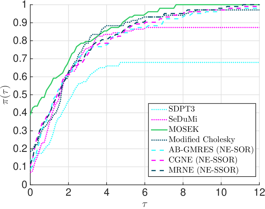


In order to show the trends of performance, we use the Dolan-Moré performance profiles [21] in Figures 1 and 2, with the proportion of problems for which -scaled performance ratio is at most , where , is the CPU time for solver to solve problem , and is the minimal CPU time for problem . Figure 1 includes the commercial solver MOSEK while Figure 2 does not. Note that the generation of Figure 2 is not by simply removing the curve of MOSEK from Figure 1, but rather removing the profile of MOSEK from the comparison dataset and thus changing the minimum CPU time cost for each problem. The comparison indicates that the iterative solvers, although slower than the commercial solver MOSEK in some cases, were often able to solve the problems to the designated accuracy.
In Tables , , and , we give the following information:
- 1.
the name of the problem and the size of the constraint matrix,
- 2.
the number of interior-point iterations required for convergence,
- 3.
CPU time for the entire computation in seconds. For the cases shorter than seconds, CPU time is taken as an average over 10 measurements. In each row, we indicate in red boldface and blue underline the fastest and second fastest solvers in CPU time, respectively.
Besides the statistics, we also use the following notation:
- †
inaccurately solved, i.e., the value of was relaxed to a larger level. In the column “Iter”, we provide extra information †a at the stopping point: for our solvers, , where is the floor function; for CVX solvers, as provided in the CVX output; PDCO solvers do not provide this information, thus they are not given;
- f
the interior-point iterations diverged;
- t
the iterations took longer than 20 hours.
Note that all zero rows and columns of the constraint matrix were removed beforehand. The problems marked with are with rank-deficient even after this preprocessing. For these problems we put in brackets after , which is computed using the Matlab function sprank.
In order to give an idea of the typical differences between methods, we present the interior-point convergence curves for problem ken_ 13. The problem has a constraint matrix with full row rank and nonzero elements.
Different aspects of the performance of the four solvers are displayed in Figure 3. The red dotted line with diamond markers represents the quantity related to AB-GMRES (NE-SOR), the blue with downward-pointing triangle CGNE (NE-SSOR), the yellow with asterisk MRNE (NE-SSOR), and the dark green with plus sign the modified Cholesky solver. Note that for this problem ken_ 13, the modified Cholesky solver became numerically inaccurate at the last step and it broke down if the default dropping tolerance was used. Thus, we increased it to .
Figure 3a shows in scale. It verifies the claim that the least squares problem becomes increasingly ill-conditioned at the final steps in the interior-point process: started from around and increased to at the last 3-5 steps. Figure 3b shows the convergence curve of the duality measure in scale. The drops below the tolerance and the stopping criterion is satisfied. Although it is not shown in the figure, we found that the interior-point method with modified Cholesky with the default value of the dropping tolerance stagnated for . Comparing with Figure 3a, it is observed that the solvers started to behave differently as increased sharply.


Figures 3c and 3d show the relative residual norm in the predictor stage and in the corrector stage, respectively. The quantities are in scale. The relative residual norm for modified Cholesky tended to increase with the interior-point iterations and sharply increased in the final phase when it lost accuracy in solving the normal equations for the steps. We observed similar trends for other test problems and, in the worst cases, the inaccuracy in the solutions prevented interior-point convergence. Among the iterative solvers, AB-GMRES (NE-SOR) and MRNE (NE-SSOR) were the most stable in keeping the accuracy of solutions to the normal equations; CGNE (NE-SSOR) performed similarly but lost numerical accuracy at the last few interior-point steps.
Figures 3e and 3f show the CPU time and number of iterations of the Krylov methods for each interior-point step, respectively. It was observed that the CPU time of the modified Cholesky solver was more evenly distributed in the whole process while that of the iterative solvers tended to be less in the beginning and ending phases. At the final stage, AB-GMRES (NE-SOR) required the fewest number of iterations but cost much more CPU time than the other two iterative solvers. This can be explained as follows: AB-GMRES (NE-SOR) requires increasingly more CPU time and memory with the number of iterations because it has to store the orthonormal vectors in the modified Gram-Schmidt process as well as the Hessenberg matrix. In contrast, CGNE (NE-SSOR) and MRNE (NE-SSOR) based methods require constant memory. CGNE (NE-SSOR) took more iterations and CPU time than MRNE (NE-SSOR). Other than and the preconditioner, the memory required for iterations of AB-GMRES is and that for CGNE and MRNE iterations is [36, 54]. This explains why AB-GMRES (NE-SOR), although requiring fewer iterations, usually takes longer to obtain the solution at each interior-point step. We also did experiments on restarting AB-GMRES for a few problems. However, the performance was not competitive compared to the non-restarted version.
On the other hand, the motivation for using AB-GMRES (NE-SOR) is that GMRES is more robust for ill-conditioned problems than the symmetric solvers CG and MINRES. This is because GMRES uses a modified Gram-Schmidt process to orthogonalize the vectors explicitly; CG and MINRES rely on short recurrences, where orthogonality of vectors may be lost due to rounding error. Moreover, GMRES allows using non-symmetric preconditioning while the symmetric solvers require symmetric preconditioning. For example, using SOR preconditioner is cheaper than SSOR for one iteration because the latter goes forwards and backwards. SOR requires 2MV + 3m operations per inner iteration, while SSOR requires 4MV + 6m. In this sense, the GMRES method has more freedom for choosing preconditioners.
From Figure 3, we may draw a few conclusions. For most problems, the direct solver gave the most efficient result in terms of CPU time. However, for some problems, the direct solver tended to lose accuracy as interior-point iterations proceeded and, in the worst cases, this would inhibit convergence. For problems where the direct method broke down, the proposed inner-iteration preconditioned Krylov subspace methods worked until convergence. With the iterative solvers, it is acceptable to solve (7) and (8) to a moderate level of accuracy in the early phase of the interior-point iterations, and then increase the level of accuracy in the late phase.
4.4 Basis pursuit problems
Most of the problems tested in the last section have a sparse constraint matrix . The average nonzero density is , , and for the problems in Netlib, Qaplib, and Mittelmann, respectively. However, the matrix can be large and dense for problems such as QP in support vector machine training and linear programming in basis pursuit [11]. The package Atomizer [10] gives such matrices.
In this section, we enrich the experiment by adding problems arising from basis pursuit [11]. We reproduced the -norm optimization problems from the package Atomizer [10], and reformulated them in the standard form of linear programming. The connection between basis pursuit and LP can be found therein. The problems tested in this section have constraint matrices with average nonzero density and are usually very well-conditioned, with condition number in the range of . The results are shown in Table 2.
0.8mm=0.77pt
| AB-GMRES | CGNE | MRNE | MOSEK | PDCO | PDCO | |||||||||
|---|---|---|---|---|---|---|---|---|---|---|---|---|---|---|
| (NE-SOR) | (NE-SSOR) | (NE-SSOR) | Direct | LSMR | ||||||||||
| Problem | Iter | Time | Iter | Time | Iter | Time | Iter | Time | Iter | Time | Iter | Time | ||
| bpfig22 | 512 | 10,240 | 8 | 141.24 | 9 | 121.68 | 9 | 117.46 | 6 | 686.02 | 14 | 33.19 | 14 | 30.50 |
| bpfig23 | 256 | 4,608 | 7 | 5.40 | 7 | 10.86 | 7 | 9.44 | 5 | 120.41 | 9 | 3.44 | 79 | 629.77 |
| bpfig24 | 256 | 2,048 | 24 | 124.83 | †-2 | † | †-7 | † | 18 | 39.85 | 28 | 13.03 | 28 | 42.20 |
| bpfig26 | 1,024 | 14,336 | 19 | 3,138.24 | †-4 | † | †-5 | † | 16 | 1,731.40 | 35 | 222.88 | 87 | 14,226.49 |
| bpfig31 | 512 | 10,240 | 8 | 136.35 | 9 | 112.73 | 9 | 118.93 | 6 | 632.10 | 14 | 35.95 | 14 | 31.61 |
| bpfig32 | 1,024 | 14,336 | 20 | 2,016.11 | †-4 | † | †-4 | † | 20 | 1,162.40 | 40 | 227.77 | f | f |
| bpfig33 | 1,024 | 22,528 | 23 | 2,507.16 | †-5 | † | †-5 | † | 26 | 1,846.84 | 41 | 231.69 | f | f |
| bpfig34 | 1,024 | 14,336 | 20 | 1,876.94 | †-4 | † | †-4 | † | 20 | 1,174.63 | 40 | 250.12 | f | f |
| bpfig41 | 256 | 4,096 | 20 | 391.63 | †-4 | † | †-4 | † | 24 | 121.53 | 32 | 11.63 | f | f |
| bpfig51 | 1,024 | 22,528 | 20 | 1,048.55 | †-5 | † | †-5 | † | 16 | 1,741.09 | 35 | 219.62 | 35 | 2,969.34 |
| bpfig52 | 256 | 2,048 | 16 | 77.93 | †-3 | † | †-2 | † | 13 | 38.39 | 28 | 9.06 | 28 | 105.90 |
| bpfig53 | 1,024 | 4,096 | 24 | 1,447.58 | †-4 | † | †-4 | † | 21 | 156.18 | 41 | 65.68 | f | f |
| bpfig54 | 1,024 | 4,096 | 22 | 1,830.62 | †-5 | † | †-6 | † | 28 | 168.20 | †-6 | † | f | f |
The notations have the same meaning as explained in the previous section. Although PDCO’s direct solver may be fast for the problems in Table 2, if the problems are given without explicit constraint matrices, one has to use the iterative solver (e.g., LSMR) version. The result shows that only AB-GMRES (NE-SOR) and MOSEK succeeded in solving all the problems. Among these two methods, AB-GMRES (NE-SOR) was faster than MOSEK for the problems bpfig22, bpfig23, bpfig31, and bpfig51.
5 Conclusions
We proposed a new way of preconditioning the normal equations of the second kind arising within interior-point methods for LP problems (11). The resulting interior-point solver is composed of three nested iteration schemes. The outer-most layer is the predictor-corrector interior-point method; the middle layer is the Krylov subspace method for least squares problems, where we may use AB-GMRES, CGNE or MRNE; on top of that, we use a row-scaling scheme that does not incur extra CPU time but helps improving the condition of the system at each interior-point step; the inner-most layer, serving as a preconditioner for the middle layer, is the stationary inner iterations. Among the three layers, only the outer-most one runs towards the required accuracy and the other two are terminated prematurely. The linear systems are solved with a gradually tightened stopping tolerance. We also proposed a new recurrence regarding in place of to omit one matrix-vector product at each interior-point step. We showed that the use of inner-iteration preconditioners in combination with these techniques enables the efficient interior-point solution of wide-ranging LP problems. We also presented a fairly extensive benchmark test for several renowned solvers including direct and iterative solvers.
The advantage of our method is that it does not break down, even when the matrices become ill-conditioned or (nearly) singular. The method is competitive for large and sparse problems and may also be well-suited to problems in which matrices are too large and dense for direct approaches to work. Extensive numerical experiments showed that our method outperforms the open-source solvers SDPT3, SeDuMi, and PDCO regarding stability and efficiency.
There are several aspects of our method that could be improved. The current implementation of the interior-point method does not use a preprocessing step except for eliminating empty rows and columns. Its efficiency may be improved by adopting some existing preprocessing procedure such as presolve to detect and remove linear dependencies of rows and columns in the constraint matrix. Also, the proposed method could be used in conjunction with more advanced interior-point frameworks such as the multi-corrector interior-point method. In terms of the linear solver, future work is to try reorthogonalization for CG and MINRES and the Householder orthogonalization for GMRES. It is also important to develop preconditioners that only require the action of the operator on a vector, as in huge basis pursuit problems.
It would also be worthwhile to extend our method to problems such as convex QP and SDP.
Acknowledgements
We would like to thank the editor and referees for their valuable comments.
References
- [1] I. Adler, M. G. C. Resende, G. Veiga, and N. Karmarkar, An implementation of Karmarkar’s algorithm for linear programming, Math. Program., 44 (1989), pp. 297–335, https://doi.org/10.1007/BF01587095.
- [2] G. Al-Jeiroudi and J. Gondzio, Convergence analysis of the inexact infeasible interior-point method for linear optimization, J. Optim. Theory Appl., 141 (2009), pp. 231–247, https://doi.org/10.1007/s10957-008-9500-5.
- [3] G. Al-Jeiroudi, J. Gondzio, and J. Hall, Preconditioning indefinite systems in interior point methods for large scale linear optimisation, Optim. Method Softw., 23 (2008), pp. 345–363, https://doi.org/10.1080/10556780701535910.
- [4] E. D. Andersen and K. D. Andersen, Presolving in linear programming, Math. Program., 71 (1995), pp. 221–245, https://doi.org/10.1007/BF01586000.
- [5] E. D. Andersen, J. Gondzio, C. Mészáros, and X. Xu, Implementation of interior-point methods for large scale linear programs, in Interior Point Methods of Mathematical Programming, P. M. Pardalos and D. Hearn, eds., vol. 5 of App. Optim., Kluwer Academic Publishers, Dordrecht, 1996, https://doi.org/10.1007/978-1-4613-3449-1_6.
- [6] L. Bergamaschi, J. Gondzio, M. Venturin, and G. Zilli, Inexact constraint preconditioners for linear systems arising in interior point methods, Comput. Optim. Appl., 36 (2007), pp. 137–147, https://doi.org/10.1007/s10589-006-9001-0.
- [7] L. Bergamaschi, J. Gondzio, and G. Zilli, Preconditioning indefinite systems in interior point methods for optimization, Comput. Optim. Appl., 28 (2004), pp. 149–171, https://doi.org/10.1023/B:COAP.0000026882.34332.1b.
- [8] Å. Björck and T. Elfving, Accelerated projection methods for computing pseudoinverse solutions of systems of linear equations, BIT, 19 (1979), pp. 145–163, https://doi.org/10.1007/BF01930845.
- [9] T. J. Carpenter and D. F. Shanno, An interior point method for quadratic programs based on conjugate projected gradients, Comput. Optim. Appl., 2 (1993), pp. 5–28, https://doi.org/10.1007/BF01299140.
- [10] S. Chen, D. Donoho, and M. Saunders, About Atomizer, 2000, http://sparselab.stanford.edu/atomizer/.
- [11] S. Chen, D. Donoho, and M. Saunders, Atomic decomposition by basis pursuit, SIAM Review, 43 (2001), pp. 129–159, https://doi.org/10.1137/S003614450037906X.
- [12] P. Chin and A. Vannelli, PCG techniques for interior point algorithms, in Proceedings of the 36th Midwest Symposium on Circuits and Systems, IEEE, 1994, pp. 200–203, https://doi.org/10.1109/MWSCAS.1993.343095.
- [13] E. J. Craig, The -step iteration procedures, J. Math. and Phys., 34 (1955), pp. 64–73, https://doi.org/10.1002/sapm195534164.
- [14] X. Cui, Approximate Generalized Inverse Preconditioning Methods for Least Squares Problems, PhD thesis, The Graduate University for Advanced Studies, Japan, 2009, http://id.nii.ac.jp/1013/00001492/.
- [15] X. Cui, K. Hayami, and J. F. Yin, Greville’s method for preconditioning least squares problems, Adv. Comput. Math., 35 (2011), pp. 243–269, https://doi.org/10.1007/s10444-011-9171-x.
- [16] J. Czyzyk, S. Mehrotra, M. Wagner, and S. J. Wright, PCx: An interior-point code for linear programming, Optim. Methods Softw., 11 (1999), pp. 397–430, https://doi.org/10.1080/10556789908805757.
- [17] M. D’Apuzzo, V. De Simone, and D. Di Serafino, On mutual impact of numerical linear algebra and large-scale optimization with focus on interior point methods, Comput. Optim. Appl., 45 (2010), pp. 283–310, https://doi.org/10.1007/s10589-008-9226-1.
- [18] T. A. Davis, CSparse: A concise sparse matrix package, 2014, http://www.suitesparse.com (accessed 2016-10-17). Version 3.1.4.
- [19] T. A. Davis and Y. Hu, The University of Florida Sparse Matrix Collection, ACM Trans. Math. Software, 38 (2011), pp. 1:1–1:25, https://doi.org/10.1145/2049662.2049663, http://www.cise.ufl.edu/research/sparse/matrices/ (accessed 2016-04-15).
- [20] A. Dax, The convergence of linear stationary iterative processes for solving singular unstructured systems of linear equations, SIAM Rev., 32 (1990), pp. 611–635, https://doi.org/10.1137/1032122.
- [21] E. D. Dolan and J. J. Moré, Benchmarking optimization software with performance profiles, Math. Program., 91 (2002), pp. 201–213, https://doi.org/10.1007/s101070100263.
- [22] I. S. Duff, MA57 — A new code for the solution of sparse symmetric definite systems, ACM Trans. Math. Softw., 30 (2004), pp. 118–144, https://doi.org/10.1145/992200.992202.
- [23] M. C. Ferris and T. S. Munson, Interior-point methods for massive support vector machines, SIAM J. Optim., 13 (2002), pp. 783–804, https://doi.org/10.1137/S1052623400374379.
- [24] R. Fourer and S. Mehrotra, Solving symmetric indefinite systems in an interior-point method for linear programming, Math. Program., 62 (1993), pp. 15–39, https://doi.org/10.1007/BF01585158.
- [25] R. W. Freund and F. Jarre, A QMR-based interior-point algorithm for solving linear programs, Math. Program., 76 (1997), pp. 183–210, https://doi.org/10.1007/BF02614383.
- [26] R. W. Freund, F. Jarre, and S. Mizuno, Convergence of a class of inexact interior-point algorithms for linear programs, Math. Oper. Res., 24 (1999), pp. 50–71, https://doi.org/10.1287/moor.24.1.50.
- [27] P. E. Gill, W. Murray, M. A. Saunders, J. A. Tomlin, and M. H. Wright, On projected Newton barrier methods for linear programming and an equivalence to Karmarkar’s projective method, Math. Program., 36 (1986), pp. 183–209, https://doi.org/10.1007/BF02592025.
- [28] J. Gondzio, HOPDM (version 2.12) — A fast LP solver based on a primal-dual interior point method, Eur. J. Oper. Res., 85 (1995), pp. 221–225, https://doi.org/10.1016/0377-2217(95)00163-K, http://www.maths.ed.ac.uk/~gondzio/software/hopdm.html.
- [29] J. Gondzio, Multiple centrality corrections in a primal-dual method for linear programming, Comput. Optim. Appl., 6 (1996), pp. 137–156, https://doi.org/10.1007/BF00249643.
- [30] J. Gondzio, Presolve analysis of linear programs prior to applying an interior point method, INFORMS J. Comput., 9 (1997), pp. 73–91, https://doi.org/10.1287/ijoc.9.1.73.
- [31] J. Gondzio, Interior point methods 25 years later, Eur. J. Oper. Res., 218 (2012), pp. 587–601, https://doi.org/10.1016/j.ejor.2011.09.017.
- [32] J. Gondzio, Matrix-free interior point method, Comput. Optim. Appl., 51 (2012), pp. 457–480, https://doi.org/10.1007/s10589-010-9361-3.
- [33] J. Gondzio and T. Terlaky, A computational view of interior point methods, in Advances in Linear and Integer Programming, J. E. Beasley, ed., Oxford University Press, Oxford, 1996, pp. 103–144, http://dl.acm.org/citation.cfm?id=247975.247978 (accessed 2016-04-15).
- [34] M. Grant and S. Boyd, CVX: Matlab software for Disciplined Convex Programming, March 2014, http://cvxr.com/cvx (accessed 2016-04-15). version 2.1.
- [35] M. C. Grant and S. P. Boyd, Graph implementations for nonsmooth convex programs, in Recent Advances in Learning and Control, V. Blondel, S. Boyd, and H. Kimura, eds., Lecture Notes in Control and Information Sciences, Springer-Verlag Limited, 2008, pp. 95–110, https://doi.org/10.1007/978-1-84800-155-8_7.
- [36] K. Hayami, J. F. Yin, and T. Ito, GMRES methods for least squares problems, SIAM J. Matrix Anal. Appl., 31 (2010), pp. 2400–2430, https://doi.org/10.1137/070696313.
- [37] M. R. Hestenes and E. Stiefel, Methods of conjugate gradients for solving linear systems, J. Research Nat. Bur. Standards, 49 (1952), pp. 409–436, https://doi.org/10.6028/jres.049.044.
- [38] J. J. Júdice, J. Patricio, L. F. Portugal, M. G. C. Resende, and G. Veiga, A study of preconditioners for network interior point methods, Comput. Optim. Appl., 24 (2003), pp. 5–35, https://doi.org/10.1023/A:1021882330897.
- [39] N. Karmarkar and K. Ramakrishnan, Computational results of an interior point algorithm for large scale linear programming, Math. Program., 52 (1991), pp. 555–586, https://doi.org/10.1007/BF01582905.
- [40] M. Kojima, S. Mizuno, and A. Yoshise, A polynomial-time algorithm for a class of linear complementarity problems, Math. Program., 4 (1989), pp. 1–26, https://doi.org/10.1007/BF01587074.
- [41] J. Korzak, Convergence analysis of inexact infeasible-interior-point algorithms for solving linear programming problems, SIAM J. Optim., 11 (2000), pp. 133–148, https://doi.org/10.1137/S1052623497329993.
- [42] I. J. Lustig, R. E. Marsten, and D. F. Shanno, On implementing Mehrotra’s predictor-corrector interior-point method for linear programming, SIAM J. Optim., 2 (1992), pp. 435–449, https://doi.org/10.1137/0802022.
- [43] I. J. Lustig, R. E. Marsten, and D. F. Shanno, Interior point methods for linear programming: Computational state of the art, ORSA J. Comput., 6 (1994), pp. 1–14, https://doi.org/10.1287/ijoc.6.1.1.
- [44] S. Mehrotra, Implementations of affine scaling methods: approximate solutions of systems of linear equations using preconditioned conjugate gradient methods, ORSA Journal on Computing, 4 (1992), pp. 103–118, https://doi.org/10.1287/ijoc.4.2.103.
- [45] S. Mehrotra, On the implementation of a primal-dual interior point method, SIAM J. Optim., 2 (1992), pp. 575–601, https://doi.org/10.1137/0802028.
- [46] S. Mehrotra and Z. Li, Convergence conditions and Krylov subspace-based corrections for primalual interior-point method, SIAM J. Optim., 15 (2005), pp. 635–653, https://doi.org/10.1137/S1052623403431494.
- [47] S. Mehrotra and J. Wang, Conjugate gradient based implementation of interior point methods for network flow problems, in Linear and nonlinear conjugate gradient-related methods, L. Adams and J. Nazareth, eds., SIAM, Philadelphia, PA, 1996, pp. 124–142.
- [48] R. D. C. Monteiro and I. Adler, Interior path following primal-dual algorithms. Part I: Linear programming, Math. Program., 44 (1989), pp. 27–41, https://doi.org/10.1007/BF01587075.
- [49] R. D. C. Monteiro and J. W. O’Neal, Convergence analysis of a long-step primal-dual infeasible interior-point LP algorithm based on iterative linear solvers, tech. report, Georgia Institute of Technology, 2003, http://www.optimization-online.org/DB_FILE/2003/10/768.pdf (accessed 2016-04-15).
- [50] R. D. C. Monteiro, J. W. O’Neal, and T. Tsuchiya, Uniform boundedness of a preconditioned normal matrix used in interior-point methods, SIAM J. Optim., 15 (2004), pp. 96–100, https://doi.org/10.1137/S1052623403426398.
- [51] K. Morikuni, Symmetric inner-iteration preconditioning for rank-deficient least squares problems, arXiv prepr., arXiv:1504.00889 (2015), pp. 1–15.
- [52] K. Morikuni, Inner-iteration preconditioning with symmetric splitting matrices for symmetric singular linear systems, Trans. JSIAM, 29 (2019), pp. 62–77, https://doi.org/10.11540/jsiamt.29.1_62.
- [53] K. Morikuni and K. Hayami, Inner-iteration Krylov subspace methods for least squares problems, SIAM J. Matrix Anal. Appl., 34 (2013), pp. 1–22, https://doi.org/10.1137/110828472.
- [54] K. Morikuni and K. Hayami, Convergence of inner-iteration GMRES methods for rank-deficient least squares problems, SIAM J. Matrix Anal. Appl., 36 (2015), pp. 225–250, https://doi.org/10.1137/130946009.
- [55] K. Morikuni and K. Hayami, Matlab-MEX Codes of the AB-GMRES Method Preconditioned by NE-SOR Inner Iterations, http://researchmap.jp/KeiichiMorikuni/Implementations/.
- [56] MOSEK ApS, The MOSEK optimization toolbox for MATLAB manual, 2015, http://docs.mosek.com/7.0/toolbox/ (accessed 2016-04-15). Version 7.1 (Revision 35).
- [57] A. R. L. Oliveira and D. C. Sorensen, A new class of preconditioners for large-scale linear systems from interior point methods for linear programming, Linear Algebra Appl., 394 (2005), pp. 1–24, https://doi.org/10.1016/j.laa.2004.08.019.
- [58] C. C. Paige and M. A. Saunders, Solution of sparse indefinite systems of linear equations, SIAM J. Numer. Anal., 12 (1975), pp. 617–629, https://doi.org/10.1137/0712047.
- [59] L. F. Portugal, M. G. C. Resende, G. Veiga, and J. J. Júdice, A truncated primal-infeasible dual-feasible network interior point method, Networks, 35 (2000), pp. 91–108, https://doi.org/10.1002/(SICI)1097-0037(200003)35:2$\langle$91::AID-NET1$\rangle$3.0.CO;2-T.
- [60] T. Rees and C. Greif, A preconditioner for linear systems arising from interior point optimization methods, SIAM J. Sci. Comput., 29 (2007), pp. 1992–2007, https://doi.org/10.1137/060661673.
- [61] M. G. C. Resende and G. Veiga, An implementation of the dual affine scaling algorithm for minimum-cost flow on bipartite uncapacitated networks, SIAM J. Optim., 3 (1993), pp. 516–537, https://doi.org/10.1137/0803025.
- [62] Y. Saad, Iterative Methods for Sparse Linear Systems, SIAM, Philadelphia, 2nd ed., 2003, https://doi.org/10.1137/1.9780898718003.
- [63] Y. Saad and M. H. Schultz, GMRES: A generalized minimal residual algorithm for solving nonsymmetric linear systems, SIAM J. Sci. Stat. Comput., 7 (1986), pp. 856–869, https://doi.org/10.1137/0907058.
- [64] M. A. Saunders, B. Kim, C. Maes, S. Akle, and M. Zahr, PDCO: Primal-dual interior method for convex objectives, 2013, http://www.stanford.edu/group/SOL/software/pdco.html.
- [65] J. F. Sturm, Using SeDuMi 1.02, a MATLAB toolbox for optimization over symmetric cones, Optim. Methods Softw., 11 (1999), pp. 625–633, https://doi.org/10.1080/10556789908805766.
- [66] K. Tanabe, Centered Newton method for mathematical programming, in System Modeling and Optimization, vol. 113 of Lecture Notes in Control and Information Sciences, Springer-Verlag, 1988, pp. 197–206, https://doi.org/10.1007/BFb0042787.
- [67] K. C. Toh, M. J. Todd, and R. H. Tütüncü, SDPT3 — a Matlab software package for semidefinite programming, Optim. Methods Softw., 11 (1999), pp. 545–581, https://doi.org/10.1080/10556789908805762.
- [68] R. H. Tütüncü, K. C. Toh, and M. J. Todd, Solving semidefinite-quadratic-linear programs using SDPT3, Math. Program. Ser. B, 95 (2003), pp. 189–217, https://doi.org/10.1007/s10107-002-0347-5.
- [69] W. Wang and D. P. O’leary, Adaptive use of iterative methods in predictor-corrector interior point methods for linear programming, Numer. Algorithms, 25 (2000), pp. 387–406, https://doi.org/10.1023/A:1016614603137.
- [70] S. J. Wright, Primal-Dual Interior-Point Methods, SIAM, Philadelphia, 1997, https://doi.org/10.1137/1.9781611971453.
- [71] S. J. Wright, Modified Cholesky factorizations in interior-point algorithms for linear programming, SIAM J. Optim., 9 (1999), pp. 1159–1191, https://doi.org/10.1137/S1052623496304712.
- [72] Y. Zhang, On the convergence of a class of infeasible interior-point methods for the horizontal linear complementary problem, SIAM J. Optim., 4 (1994), pp. 208–227, https://doi.org/10.1137/0804012.
- [73] Y. Zhang, Solving large-scale linear programs by interior-point methods under the Matlab environment, Optim. Methods Softw., 10 (1998), pp. 1–31, https://doi.org/10.1080/10556789808805699.