跳到论文正文
W Papers独立论文阅读器 arXiv:1604.07458 论文正文 计算阅读时间 · 0%
引用这篇论文根据当前论文元数据生成,正式投稿前建议核对。


License: arXiv.org perpetual non-exclusive license
arXiv:1604.07458v1 [cond-mat.quant-gas] 25 Apr 2016

Second-order hydrodynamics for fermionic cold atoms
—Detailed analysis of transport coefficients and relaxation times—

Preprint: KUNS-2623
Yuta Kikuchi Email: kikuchi@ruby.scphys.kyoto-u.ac.jp Affiliation: Department of Physics, Faculty of Science, Kyoto University, Kyoto 606-8502, Japan.    Kyosuke Tsumura Email: kyosuke.tsumura@fujifilm.com Affiliation: Analysis Technology Center, Research & Development Management Headquarters, Fujifilm Corporation, Kanagawa 250-0193, Japan.    Teiji Kunihiro Email: kunihiro@ruby.scphys.kyoto-u.ac.jp Affiliation: Department of Physics, Faculty of Science, Kyoto University, Kyoto 606-8502, Japan.
August 24, 2026
Abstract

We give a detailed derivation of the second-order (local) hydrodynamics for Boltzmann equation with an external force by using the renormalization group method. In this method, we solve the Boltzmann equation faithfully to extract the hydrodynamics without recourse to any ansatz. Our method leads to microscopic expressions of not only all the transport coefficients that are of the same form as those in Chapman-Enskog method but also those of the viscous relaxation times τi\tau_{i} that admit physically natural interpretations. As an example, we apply our microscopic expressions to calculate the transport coefficients and the relaxation times of the cold fermionic atoms in a quantitative way, where the transition probability in the collision term is given explicitly in terms of the ss-wave scattering length asa_{s}. We thereby discuss the quantum statistical effects, temperature dependence, and scattering-length dependence of the first-order transport coefficients and the viscous relaxation times: It is shown that as the temperature is lowered, the transport coefficients and the relaxation times increase rapidly because Pauli principle acts effectively. On the other hand, as asa_{s} is increased, these quantities decrease and become vanishingly small at unitarity because of the strong coupling. The numerical calculation shows that the relation τπ=η/P\tau_{\pi}=\eta/P, which is derived in the relaxation-time approximation and used in most of literature without almost any foundation, turns out to be satisfied quite well, while the similar relation for the relaxation time τJ\tau_{J} of the heat conductivity is satisfied only approximately with a considerable error.

pacs
05.10.Cc, 25.75.-q, 47.75.+f

I Introduction

The hydrodynamic equation is expressed in terms of macroscopic quantities such as the pressure, particle number density, and fluid velocity, and takes a universal form irrespective of the microscopic dynamics of the system. The detailed microscopic properties of the system are renormalized into transport coefficients such as the shear viscosity, heat conductivity and so on. Therefore, the elaborate investigation of the transport coefficients is one of the most important tasks to reveal the microscopic properties of the fluid. For instance, the fluid with a tiny shear viscosity is realized in the experiment of ultracold Fermi gases at the unitarity [1, 2, 3, 4, 5, 6]: The value of its shear viscosity is close to a quantum bound that is theoretically proposed [7, 8], implying the realization of the strongly correlated systems at the unitarity [9, 10, 11, 12, 13, 14]. The hydrodynamic behavior with a small shear viscosity is also discovered in the ultra-relativistic heavy ion collision experiments at the Relativistic Heavy Ion Collider (RHIC) at the Brookhaven National Laboratory and the Large Hadron Collider (LHC) at CERN, which may again suggest that the created matter, i.e., Quark-gluon plasma (QGP) is a strongly coupled system (see Refs. [15, 16], for instance). It is noteworthy that, in spite of very large difference of the energy scale, these systems share common hydrodynamic properties, and the hydrodynamic equation provides us with a unified way to study their dynamics.

However, there is a problem in the application of the Navier-Stokes equation, besides the causality problem typical to the relativistic hydrodynamics: In finite systems, there are the central region where the density is large enough to apply the naive viscous hydrodynamic equation, and the peripheral region where the naive hydrodynamic description breaks down due to the small density. In the latter, since the system slowly approaches the thermal equilibrium state due to the lack of enough collision rate, we need to take into account more microscopic dynamics. To this end, we should incorporate the relaxation process of dissipative currents, which is characterized by viscous relaxation times [17, 18, 10, 19, 20, 21]. The second-order hydrodynamic equation describes the mesoscopic dynamics including the relaxation of the dissipative currents, in addition to the ordinary hydrodynamic behavior described by the Navier-Stokes equation. It should be emphasized that, though the importance of the second-order hydrodynamics has been recognized and many attempts has been done to derive it, its formulation is still controversial [22, 23, 24, 25, 26, 27].

In this paper, we derive the second-order hydrodynamic equation from the Boltzmann equation for non-relativistic systems by using the renormalization group (RG) method [28, 29, 30, 31, 32, 33, 34, 35, 36, 37, 38, 39, 40]. In the RG method, we faithfully solve the Boltzmann equation and extract the hydrodynamics as a low-energy effective dynamics of the kinetic theory. It has been applied to derive the first- and second-order hydrodynamic equations for both relativistic and non-relativistic systems [38, 41, 42, 43, 44, 45], and desirable properties have been already shown for the resultant equation such as causality, stability, positivity of the entropy production rate, and the Onsager’s reciprocal relation without imposing any assumption a priori [45, 46]. Moreover, the microscopic expressions obtained for the transport coefficients such as the shear viscosity, heat conductivity and so on coincide with those derived in the celebrated Chapman-Enskog method, while the novel microscopic expressions of the viscous relaxation times written in terms of the relaxation functions allow physically natural interpretations as the relaxation times. As an extension of Ref. [44], we take account of the effect of quantum statistics and external forces. As an application, we use our microscopic expressions to calculate the shear viscosity, heat conductivity, and viscous relaxation times of the stress tensor and heat flow of the cold fermionic atoms in a quantitative way, where the transition amplitude in the collision term is given explicitly in terms of the ss-wave scattering length asa_{s}: The microscopic expressions given in forms of correlation functions are converted to linear integral equations, which we solve numerically without recourse to any approximation. On the basis of the numerical results, we discuss the quantum statistical effects, temperature dependence, and scattering-length dependence of the first-order transport coefficients and the viscous relaxation times: It is shown that at low temperatures, quantum statistics acts so effectively that the transport coefficients and the relaxation times increase rapidly because Pauli principle almost forbids particle scatterings other than the forward ones. On the other hand, as asa_{s} is increased up to unitarity, these quantities decrease monotonically and become vanishingly small at unitarity because of the strong coupling. We also examine how well the relation τπ=η/P\tau_{\pi}=\eta/P and its analog for the heat conductivity are satisfied, where τπ\tau_{\pi} is the viscous relaxation time of the stress tensor, η\eta the shear viscosity, and PP the pressure. These relations are obtained from the Boltzmann equation with use of the relaxation-time approximation (RTA), which has been widely applied to a lot of studies of the kinetic theory [19, 20, 21]. Although the RTA might happen to be valid for a system close to the local equilibrium, its quantitative reliability is unclear and has been hardly checked even apart from the fact that the relaxation times should have different values depending on the realization process: We are only aware of [47] in which the validity of the RTA is analytically examined up to some approximations. We show that the relation τπ=η/P\tau_{\pi}=\eta/P holds quite well, while the similar relation for the relaxation time τJ\tau_{J} of the heat conductivity is satisfied only approximately with a considerable error. Here we should mention that a brief report of the present work is already given in Ref. [48], and the present paper give the detailes of not only the analytic but also numerical calculations.

This paper is organized as follows: In Sec. II, we briefly summarize the properties of the Boltzmann equation. In Sec. III, we derive the second-order hydrodynamic equation by using RG method, and show the resultant equations and microscopic expressions of the transport coefficients. In Sec. IV, we reduce the microscopic expressions of the transport coefficients and the viscous relaxation times for the numerical calculations. In Sec. V, we show the numerical results of the transport coefficients and the viscous relaxation times, and discuss the physical properties of the numerical results with temperature and the scattering length being varied. Convergence of the numerical results are confirmed in the last part of this section. In Sec. VI, we give the concluding remarks. In Appendix. A, we give a useful formula which is used to solve the Boltzmann equation. In Appendix. B, we present the detailed derivation of the relaxation equation.

II Boltzmann equation

In this section, we give a brief review of the Boltzmann equation and its properties. The Boltzmann equation, which describes the time-evolution of the one-body distribution function fp​(t,𝒙)f_{p}(t,\boldsymbol{x}) in the phase space, takes the following form:

(∂∂t+𝒗⋅∇+𝑭⋅∇p)fp(t,𝒙)=C[f]p(t,𝒙),\displaystyle\left(\frac{\partial}{\partial t}+\boldsymbol{v}\cdot\boldsymbol{\nabla}+\boldsymbol{F}\cdot\boldsymbol{\nabla}_{p}\right)f_{p}(t,\boldsymbol{x})=C[f]_{p}(t,\boldsymbol{x}), (1)

with 𝒗≡𝒑/(2​m)\boldsymbol{v}\equiv\boldsymbol{p}/(2m) and the collision integral given by

C​[f]p​(t,𝒙)\displaystyle C[f]_{p}(t,\boldsymbol{x}) =12∫p1∫p2∫p3𝒲(p,p1|p2,p3)(f¯pf¯p1fp2fp3−fpfp1f¯p2f¯p3).\displaystyle=\frac{1}{2}\int_{p_{1}}\int_{p_{2}}\int_{p_{3}}\mathcal{W}(p,p_{1}|p_{2},p_{3})\big(\bar{f}_{p}\bar{f}_{p_{1}}f_{p_{2}}f_{p_{3}}-f_{p}f_{p_{1}}\bar{f}_{p_{2}}\bar{f}_{p_{3}}\big). (2)

Here, we have introduced the notations ∫p≡∫d3p/(2π)3\int_{p}\equiv\int\mathrm{d}^{3}p/(2\pi)^{3} and f¯≡1+a​f\bar{f}\equiv 1+af. aa represents quantum statistics, i.e., a=−1​(+1)a=-1(+1) for fermion (boson) and a=0a=0 for the classical Boltzmann gas. 𝑭\boldsymbol{F} represents the external force which particles experience. In this paper, we consider the force driven by the scalar potential, 𝑭=−∇Ep\boldsymbol{F}=-\boldsymbol{\nabla}E_{p} with Ep=|𝒑|2/(2​m)+V⁡(𝒙)E_{p}=|\boldsymbol{p}|^{2}/(2m)+V(\boldsymbol{x}), where any inhomogeneous mean fields may be incorporated into the potential VV. 𝒲\mathcal{W} is a transition matrix given by

𝒲\displaystyle\mathcal{W} =|ℳ|2​(2​π)4​δ​(Ep+Ep1−Ep2−Ep3)​δ3​(𝒑+𝒑1−𝒑2−𝒑3),\displaystyle=|\mathcal{M}|^{2}(2\pi)^{4}\delta(E_{p}+E_{p_{1}}-E_{p_{2}}-E_{p_{3}})\delta^{3}(\boldsymbol{p}+\boldsymbol{p}_{1}-\boldsymbol{p}_{2}-\boldsymbol{p}_{3}), (3)

with the scattering amplitude ℳ\mathcal{M}. The transition matrix has the following symmetries

𝒲(p,p1|p2,p3)=𝒲(p2,p3|p,p1)=𝒲(p1,p|p3,p2)=𝒲(p3,p2|p1,p).\displaystyle\mathcal{W}(p,p_{1}|p_{2},p_{3})=\mathcal{W}(p_{2},p_{3}|p,p_{1})=\mathcal{W}(p_{1},p|p_{3},p_{2})=\mathcal{W}(p_{3},p_{2}|p_{1},p). (4)

By using these symmetries one finds that the following identity is satisfied for an arbitrary spacetime dependent vector Φp​(x)\Phi_{p}(x):

∫pΦp​C​[f]p\displaystyle\int_{p}\Phi_{p}C[f]_{p} =18∫p∫p1∫p2∫p3𝒲(p,p1|p2,p3)\displaystyle=\frac{1}{8}\int_{p}\int_{p_{1}}\int_{p_{2}}\int_{p_{3}}\mathcal{W}(p,p_{1}|p_{2},p_{3})
×(Φp+Φp1−Φp2−Φp3)​(f¯p​f¯p1​fp2​fp3−fp​fp1​f¯p2​f¯p3).\displaystyle\times\big(\Phi_{p}+\Phi_{p_{1}}-\Phi_{p_{2}}-\Phi_{p_{3}}\big)\big(\bar{f}_{p}\bar{f}_{p_{1}}f_{p_{2}}f_{p_{3}}-f_{p}f_{p_{1}}\bar{f}_{p_{2}}\bar{f}_{p_{3}}\big). (5)

When Φp\Phi_{p} vanishes Eq. (5), Φp\Phi_{p} is called a collision invariant, and any linear combination of conserved quantities, i.e., the particle number, momenta, and energy, is found to be a collision invariant. Accordingly, Φp=α+𝜷⋅𝒑+γ​Ep≡Φpinv​(x)\Phi_{p}=\alpha+\boldsymbol{\beta}\cdot\boldsymbol{p}+\gamma E_{p}\equiv\Phi_{p}^{\rm inv}(x) with the space-time dependent coefficients α\alpha, 𝜷\boldsymbol{\beta} and γ\gamma is a collision invariant.

In the Boltzmann theory, the entropy density and current are defined by

{s,𝑱s}≡−∫p{1,𝒗}(fplnfp−f¯p​ln⁡f¯pa),\displaystyle\{s,\boldsymbol{J}_{s}\}\equiv-\int_{p}\{1,\boldsymbol{v}\}\left(f_{p}\ln f_{p}-\frac{\bar{f}_{p}\ln\bar{f}_{p}}{a}\right), (6)

which satisfies

∂s∂t+∇⋅𝑱s\displaystyle\frac{\partial s}{\partial t}+\boldsymbol{\nabla}\cdot\boldsymbol{J}_{s} =−∫pln(fpf¯p)(∂fp∂t+𝒗⋅∇fp)=−∫pln(fpf¯p)C[f]p.\displaystyle=-\int_{p}\ln\left(\frac{f_{p}}{\bar{f}_{p}}\right)\left(\frac{\partial f_{p}}{\partial t}+\boldsymbol{v}\cdot\boldsymbol{\nabla}f_{p}\right)=-\int_{p}\ln\left(\frac{f_{p}}{\bar{f}_{p}}\right)C[f]_{p}. (7)

In the second equality, we have utilized the fact that the force term does not contribute as

∫pln⁡(fpf¯p)​𝑭⋅∇pfp\displaystyle\int_{p}\ln\left(\frac{f_{p}}{\bar{f}_{p}}\right)\boldsymbol{F}\cdot\boldsymbol{\nabla}_{p}f_{p} =−𝑭⋅∫pfp∇pln(fpf¯p)=−𝑭⋅∫pfp(∇pfpfp−a​∇p​fpf¯p)\displaystyle=-\boldsymbol{F}\cdot\int_{p}f_{p}{\boldsymbol{\nabla}}_{p}\ln\left(\frac{f_{p}}{\bar{f}_{p}}\right)=-\boldsymbol{F}\cdot\int_{p}f_{p}\left(\frac{{\boldsymbol{\nabla}}_{p}f_{p}}{f_{p}}-\frac{a{\boldsymbol{\nabla}}_{p}f_{p}}{\bar{f}_{p}}\right)
=−𝑭⋅∫p∇pfpf¯p=−1a𝑭⋅∫p∇plnf¯p=0.\displaystyle=-\boldsymbol{F}\cdot\int_{p}\frac{{\boldsymbol{\nabla}}_{p}f_{p}}{\bar{f}_{p}}=-\frac{1}{a}\boldsymbol{F}\cdot\int_{p}\boldsymbol{\boldsymbol{\nabla}}_{p}\ln\bar{f}_{p}=0. (8)

where 𝑭\boldsymbol{F} is assumed to be independent of momentum and we have neglected surface terms. From Eq. (7), one finds that entropy is conserved if ln⁡(fp/f¯p)\ln(f_{p}/\bar{f}_{p}) is a collision invariant Φpinv​(x)\Phi_{p}^{\rm inv}(x), i.e., fp=1/[e−Φpinv​(x)−a]f_{p}=1/[\mathrm{e}^{-\Phi_{p}^{\rm inv}(x)}-a], which is reduced to the form of a local equilibrium distribution function,

fpst\displaystyle f^{\mathrm{st}}_{p} =1e(m​|𝒗−𝒖|2/2+V−μ)/T−a=1e(|𝜹​𝒑|2/(2​m)+V−μ)/T−a.\displaystyle=\frac{1}{\mathrm{e}^{(m|\boldsymbol{v}-\boldsymbol{u}|^{2}/2+V-\mu)/T}-a}=\frac{1}{\mathrm{e}^{(|\boldsymbol{\delta p}|^{2}/(2m)+V-\mu)/T}-a}. (9)

Here we have introduced the relative momentum 𝜹​𝒑\boldsymbol{\delta p}. The relative momentum 𝜹​𝒑\boldsymbol{\delta p} and relative velocity 𝜹​𝒗\boldsymbol{\delta v} against the fluid velocity 𝒖\boldsymbol{u} are defined by 𝜹​𝒑≡m​𝜹​𝒗≡m​𝒗−m​𝒖\boldsymbol{\delta p}\equiv m\boldsymbol{\delta v}\equiv m\boldsymbol{v}-m\boldsymbol{u}.

III Derivation of hydrodynamics

The RG method is a general framework to identify (fewer) slow variables and extract their dynamics from the original complicated dynamics [28, 30, 31, 36]. In this section, we solve the Boltzmann equation (1) to derive the second-order hydrodynamic equation by applying the RG method. The key to extract mesoscopic dynamics in addition to the slowest macroscopic dynamics is how to identify the excited modes, which is realized by utilizing the doublet scheme [44, 45] to which we refer the details of the RG method applied to Boltzmann equation to extract hydrodynamics, although any mean field is not included in the Boltzmann equation there.

III.1 Solving the Boltzmann equation

We perform the perturbative calculation assuming that the mean free path is much smaller than the spatial variation of the potential term. We introduce the bookkeeping parameter ϵ\epsilon to the Boltzmann equation (1),

(∂∂t+ϵ𝒗⋅∇+ϵ𝑭⋅∇p)fp(t,𝒙)=C[f]p(t,𝒙).\displaystyle\left(\frac{\partial}{\partial t}+\epsilon\boldsymbol{v}\cdot\boldsymbol{\nabla}+\epsilon\boldsymbol{F}\cdot\boldsymbol{\nabla}_{p}\right)f_{p}(t,\boldsymbol{x})=C[f]_{p}(t,\boldsymbol{x}). (10)

The parameter ϵ\epsilon is interpreted as the Knudsen number defined by (mean free path)//(macroscopic length scale). Note that the external force is also assumed to be as small as spatial inhomogeneity since it is caused by the spatial variation of the external potential.

We expand the distribution function in the following perturbation series with respect to ϵ\epsilon,

f~​(t,t0)=f~(0)​(t,t0)+ϵ​f~(1)​(t,t0)+ϵ2​f~(2)​(t,t0)+𝒪⁡(ϵ3),\displaystyle\tilde{f}(t;t_{0})=\tilde{f}^{(0)}(t;t_{0})+\epsilon\tilde{f}^{(1)}(t;t_{0})+\epsilon^{2}\tilde{f}^{(2)}(t;t_{0})+\mathcal{O}(\epsilon^{3}), (11)

and solve the Boltzmann equation order by order under the initial condition,

f~​(t=t0)\displaystyle\tilde{f}(t=t_{0}) =f⁡(t=t0)=f(0)​(t0)+ϵ​f(1)​(t0)+ϵ2​f(2)​(t0)+𝒪⁡(ϵ3),\displaystyle=f(t=t_{0})=f^{(0)}(t_{0})+\epsilon f^{(1)}(t_{0})+\epsilon^{2}f^{(2)}(t_{0})+\mathcal{O}(\epsilon^{3}), (12)

which is taken to be an exact solution of the Boltzmann equation (10).

The zeroth order equation with respect to ϵ\epsilon reads

∂∂t​f~p(0)​(t,t0)=C​[f~(0)]p​(t,t0).\displaystyle\frac{\partial}{\partial t}\tilde{f}_{p}^{(0)}(t;t_{0})=C[\tilde{f}^{(0)}]_{p}(t;t_{0}). (13)

Since we are interested in a slow motion in the asymptotic regime, we seek for the solution of the following equation,

∂∂t​f~p(0)​(t,t0)=0,\displaystyle\frac{\partial}{\partial t}\tilde{f}_{p}^{(0)}(t;t_{0})=0, (14)

which is equivalent to

C​[f~(0)]p​(t,t0)=0.\displaystyle C[\tilde{f}^{(0)}]_{p}(t;t_{0})=0. (15)

This equation leads to the condition

f¯p​f¯p1​fp2​fp3=fp​fp1​f¯p2​f¯p3.\displaystyle\bar{f}_{p}\bar{f}_{p_{1}}f_{p_{2}}f_{p_{3}}=f_{p}f_{p_{1}}\bar{f}_{p_{2}}\bar{f}_{p_{3}}. (16)

By taking logarithm of both sides of this equation we note that the equation requires that ln⁡(fp/f¯p)\ln(f_{p}/\bar{f}_{p}) should become a linear combination of {1,𝒑,E}\{1,\boldsymbol{p},E\} the coefficients which are constant in time tt but may depend on the space coordinate 𝒙\boldsymbol{x} and the initial time t0t_{0}. From the discussion in the last section, we see that the zeroth order solution takes the form of a local equilibrium distribution function,

f~p(0)​(t,t0)=fpeq​(t0)=(exp⁡[(m/2)​|𝒗−𝒖⁡(t0,𝒙)|2−μTF​(t0,𝒙)T⁡(t0,𝒙)]−a)−1,\displaystyle\tilde{f}_{p}^{(0)}(t;t_{0})=f^{\mathrm{eq}}_{p}(t_{0})=\left(\exp\left[\frac{(m/2)|\boldsymbol{v}-\boldsymbol{u}(t_{0},\boldsymbol{x})|^{2}-\mu_{\mathrm{TF}}(t_{0},\boldsymbol{x})}{T(t_{0},\boldsymbol{x})}\right]-a\right)^{-1}, (17)

where we have defined μT​F​(t0,𝒙)=μ⁡(t0,𝒙)−V⁡(𝒙)\mu_{TF}(t_{0},\boldsymbol{x})=\mu(t_{0},\boldsymbol{x})-V(\boldsymbol{x}). Five integration constants T⁡(t0,𝒙)T(t_{0},\boldsymbol{x}), 𝒖⁡(t0,𝒙)\boldsymbol{u}(t_{0},\boldsymbol{x}), and μ⁡(t0,𝒙)\mu(t_{0},\boldsymbol{x}) are would-be temperature, fluid velocity, and chemical potential, which will be lifted to dynamical variables eventually to characterize the slowest dynamics of resultant hydrodynamics.

Next, we consider the first order equation:

∂∂t​f~(1)​(t)=feq​f¯eq​L​(feq​f¯eq)−1​f~(1)​(t)+feq​f¯eq​F0,\displaystyle\frac{\partial}{\partial t}\tilde{f}^{(1)}(t)=f^{\mathrm{eq}}\bar{f}^{\mathrm{eq}}L(f^{\mathrm{eq}}\bar{f}^{\mathrm{eq}})^{-1}\tilde{f}^{\mathrm{(1)}}(t)+f^{\mathrm{eq}}\bar{f}^{\mathrm{eq}}F_{0}, (18)

with the initial condition

f~(1)​(t=t0,t0)=f(1)​(t0)≡feq​f¯eq​Ψ​(t0).\displaystyle\tilde{f}^{(1)}(t=t_{0},t_{0})=f^{(1)}(t_{0})\equiv f^{\mathrm{eq}}\bar{f}^{\mathrm{eq}}\Psi(t_{0}). (19)

Ψ⁡(t0)\Psi(t_{0}) is to be determined later. Here, the linearized collision operator LL and the inhomogeneous term F0F_{0} are defined by

Lp​q\displaystyle L_{pq} ≡(fpeq​f¯peq)−1​δδ​fq​C​[f]p​(t)|f=feq​fqeq​f¯qeq\displaystyle\equiv(f^{\mathrm{eq}}_{p}\bar{f}^{\mathrm{eq}}_{p})^{-1}\left.\frac{\delta}{\delta f_{q}}C[f]_{p}(t)\right|_{f=f^{\mathrm{eq}}}f^{\mathrm{eq}}_{q}\bar{f}^{\mathrm{eq}}_{q}
=−12​f¯peq∫p1∫p2∫p3𝒲(p,p1|p2,p3)fp1eqf¯p2eqf¯p3eq\displaystyle=-\frac{1}{2\bar{f}^{\mathrm{eq}}_{p}}\int_{p_{1}}\int_{p_{2}}\int_{p_{3}}\mathcal{W}(p,p_{1}|p_{2},p_{3})f^{\mathrm{eq}}_{p_{1}}\bar{f}^{\mathrm{eq}}_{p_{2}}\bar{f}^{\mathrm{eq}}_{p_{3}}
×[δ3​(𝒑−𝒒)+δ3​(𝒑𝟏−𝒒)−δ3​(𝒑𝟐−𝒒)−δ3​(𝒑𝟑−𝒒)],\displaystyle\times\big[\delta^{3}(\boldsymbol{p}-\boldsymbol{q})+\delta^{3}(\boldsymbol{p_{1}}-\boldsymbol{q})-\delta^{3}(\boldsymbol{p_{2}}-\boldsymbol{q})-\delta^{3}(\boldsymbol{p_{3}}-\boldsymbol{q})\big], (20)
Fi​p\displaystyle F_{ip} ≡F[f~(i)]p≡−(fpeqf¯peq)−1(𝒗⋅∇+𝑭⋅∇p)f~p(i).\displaystyle\equiv F[\tilde{f}^{(i)}]_{p}\equiv-(f^{\mathrm{eq}}_{p}\bar{f}^{\mathrm{eq}}_{p})^{-1}\left(\boldsymbol{v}\cdot\boldsymbol{\nabla}+\boldsymbol{F}\cdot\boldsymbol{\nabla}_{p}\right)\tilde{f}^{(i)}_{p}. (21)

For arbitrary vectors ψp\psi_{p} and χp\chi_{p}, the linearized collision operator has the following three significant properties:

⟨ψ,L​χ⟩=⟨L​ψ,χ⟩,⟨ψ,L​ψ⟩≤0,L​φα=0,\displaystyle\left<\psi,L\chi\right>=\left<L\psi,\chi\right>,\ \ \ \left<\psi,L\psi\right>\leq 0,\ \ \ L\varphi^{\alpha}=0, (22)

with the definition of the inner product given by

⟨ψ,χ⟩≡∫pfpeq​f¯peq​ψp​χp.\displaystyle\left<\psi,\chi\right>\equiv\int_{p}f^{\mathrm{eq}}_{p}\bar{f}^{\mathrm{eq}}_{p}\psi_{p}\chi_{p}. (23)

The linearized collision operator has five zero modes,

φ0​p0=1,φ0​pi=δ​pi,φ0​p4=|𝜹​𝒑|22​m−hTF,\displaystyle\varphi_{0p}^{0}=1,\ \ \ \varphi_{0p}^{i}=\delta p^{i},\ \ \ \varphi_{0p}^{4}=\frac{|\boldsymbol{\delta p}|^{2}}{2m}-h_{\mathrm{TF}}, (24)

with hTFh_{\mathrm{TF}} being the enthalpy density, the explicit form of which will be given shortly. The zero modes satisfy the orthogonality relation

⟨φ0α,φ0β⟩=cα​δα​β.\displaystyle\langle\varphi_{0}^{\alpha},\varphi_{0}^{\beta}\rangle=c^{\alpha}\delta^{\alpha\beta}. (25)

with the following normalization factors

c0\displaystyle c^{0} =T​∂n∂μTF,ci=m​n​T,c4=3​n​T2​(hTF−3​n2​(∂n∂μTF)−1).\displaystyle=T\frac{\partial n}{\partial\,\mu_{\mathrm{TF}}},\ \ \ c^{i}=mnT,\ \ \ c^{4}=\frac{3nT}{2}\left(h_{\mathrm{TF}}-\frac{3n}{2}\left(\frac{\partial n}{\partial\mu_{\mathrm{TF}}}\right)^{-1}\right). (26)

The particle number density nn and the enthalpy density hTFh_{\mathrm{TF}} are defined by

n⁡(t,𝒙)\displaystyle n(t,\boldsymbol{x}) ≡∫pfpeq​(t,𝒙),\displaystyle\equiv\int_{p}f^{\mathrm{eq}}_{p}(t,\boldsymbol{x}), (27)
hTF​(t,𝒙)\displaystyle h_{\mathrm{TF}}(t,\boldsymbol{x}) ≡h⁡(t,𝒙)−V⁡(𝒙)≡e⁡(t,𝒙)+P⁡(t,𝒙)n⁡(t,𝒙)−V⁡(𝒙).\displaystyle\equiv h(t,\boldsymbol{x})-V(\boldsymbol{x})\equiv e(t,\boldsymbol{x})+\frac{P(t,\boldsymbol{x})}{n(t,\boldsymbol{x})}-V(\boldsymbol{x}). (28)

The energy density ee and the pressure PP are given by

e⁡(t,𝒙)\displaystyle e(t,\boldsymbol{x}) ≡1n​∫pfpeq​(t,𝒙)​(|𝜹​𝒑|22​m+V⁡(𝒙)),\displaystyle\equiv\frac{1}{n}\int_{p}f^{\mathrm{eq}}_{p}(t,\boldsymbol{x})\left(\frac{|\boldsymbol{\delta p}|^{2}}{2m}+V(\boldsymbol{x})\right), (30)
P⁡(t,𝒙)\displaystyle P(t,\boldsymbol{x}) ≡13​∫pfpeq​(t,𝒙)​𝜹​𝒗⋅𝜹​𝒑,\displaystyle\equiv\frac{1}{3}\int_{p}f^{\mathrm{eq}}_{p}(t,\boldsymbol{x})\boldsymbol{\delta v}\cdot\boldsymbol{\delta p}, (31)

respectively. We define P0-space and Q0-space as the space spanned by the zero modes given in Eq. (24) and its complemental space, respectively. The associated projection operators are defined as

[P0​ψ]p\displaystyle[P_{0}\psi]_{p} ≡∑α=04φ0​pαcα​⟨φ0α,ψ⟩,\displaystyle\equiv\sum_{\alpha=0}^{4}\frac{\varphi^{\alpha}_{0p}}{c^{\alpha}}\langle\varphi_{0}^{\alpha},\psi\rangle, (32)
Q0\displaystyle Q_{0} ≡1−P0,\displaystyle\equiv 1-P_{0}, (33)

for an arbitrary vector ψp\psi_{p}. By solving the first order equation we obtain the first-order perturbative solution:

f~(1)​(t,t0)=\displaystyle\tilde{f}^{(1)}(t;t_{0})= feq​f¯eq​[e(t−t0)​L​(Ψ⁡(t0)+L−1​Q0​F0)+(t−t0)​P0​F0−L−1​Q0​F0].\displaystyle f^{\mathrm{eq}}\bar{f}^{\mathrm{eq}}\Big[\mathrm{e}^{(t-t_{0})L}(\Psi(t_{0})+L^{-1}Q_{0}F_{0})+(t-t_{0})P_{0}F_{0}-L^{-1}Q_{0}F_{0}\Big]. (34)

Though we have formally obtained the first-order solution, the initial condition has not yet been determined. The determination of Ψ\Psi is done in the following way [45]: We expand Eq. (34) up to the first-order with respect to |t−t0||t-t_{0}|,

f~(1)​(t,t0)=\displaystyle\tilde{f}^{(1)}(t;t_{0})= feq​f¯eq​[Ψ⁡(t0)+(t−t0)​(L​Ψ​(t0)+Q0​F0+P0​F0)].\displaystyle f^{\mathrm{eq}}\bar{f}^{\mathrm{eq}}\Big[\Psi(t_{0})+(t-t_{0})(L\Psi(t_{0})+Q_{0}F_{0}+P_{0}F_{0})\Big]. (35)

Such an expansion makes sense because we need only tangents of perturbative solution when applying the RG equation. Now, we require that the tangent space of the perturbative solution becomes smallest, which is realized by choosing L​Ψ​(t0)L\Psi(t_{0}) so that L​Ψ​(t0)L\Psi(t_{0}) and Q0​F0Q_{0}F_{0} belong to a common space, and we define P1-space and Q1-space by the space spanned by Eq. (35) and its complemental space, respectively. As is worked out in App. A, L−1​Q0​F0L^{-1}Q_{0}F_{0} is calculated to be

[L−1​Q0​F0]p=−σi​jT​[L−1​π^i​j]p−∇iTT2​[L−1​J^i]p,\displaystyle[L^{-1}Q_{0}F_{0}]_{p}=-\frac{\sigma^{ij}}{T}[L^{-1}\hat{\pi}^{ij}]_{p}-\frac{\nabla^{i}T}{T^{2}}[L^{-1}\hat{J}^{i}]_{p}, (36)

where we have introduced excited modes (π^pi​j,J^pi)(\hat{\pi}^{ij}_{p},\hat{J}^{i}_{p}) defined by

π^pi​j\displaystyle\hat{\pi}^{ij}_{p} ≡δv⟨iδpj⟩,J^pi≡(|𝜹​𝒑|22​m−hTF)δvi.\displaystyle\equiv\delta v^{\langle i}\delta p^{j\rangle},\ \ \ \hat{J}^{i}_{p}\equiv\left(\frac{|\boldsymbol{\delta p}|^{2}}{2m}-h_{\mathrm{TF}}\right)\delta v^{i}. (37)

Here for an arbitrary tensor AA, A⟨i​j⟩≡Δi​j​k​l​Ai​jA^{\langle ij\rangle}\equiv\Delta^{ijkl}A^{ij} with the definition of a symmetric traceless tensor Δi​j​k​l≡12​δi​k​δj​l+12​δi​l​δj​k−13​δi​j​δk​l\Delta^{ijkl}\equiv\frac{1}{2}\delta^{ik}\delta^{jl}+\frac{1}{2}\delta^{il}\delta^{jk}-\frac{1}{3}\delta^{ij}\delta^{kl}. Therefore, it is physically natural to choose Ψ⁡(t0)\Psi(t_{0}) so that it belongs to the space spanned by ([L−1π^i​j]p,L−1J^i]p)([L^{-1}\hat{\pi}^{ij}]_{p},L^{-1}\hat{J}^{i}]_{p}), and Ψ⁡(t0)\Psi(t_{0}) may be parametrized as

Ψp​(t0)=−5​[L−1​π^i​j]p⟨π^k​l,L−1​π^k​l⟩​πi​j​(t0)−3​[L−1​J^i]p⟨J^l,L−1​J^k⟩​Jk​(t0),\displaystyle\Psi_{p}(t_{0})=-5\frac{[L^{-1}\hat{\pi}^{ij}]_{p}}{\langle\hat{\pi}^{kl},L^{-1}\hat{\pi}^{kl}\rangle}\pi^{ij}(t_{0})-3\frac{[L^{-1}\hat{J}^{i}]_{p}}{\langle\hat{J}^{l},L^{-1}\hat{J}^{k}\rangle}J^{k}(t_{0}), (38)

with eight would-be integral constants πi​j​(t0)\pi^{ij}(t_{0}) and Ji​(t0)J^{i}(t_{0}), which will be identified as the stress tensor and heat flow, respectively. From Eq. (35), P1-space is found to be spanned by doublet modes (π^pi​j,J^pi)(\hat{\pi}^{ij}_{p},\hat{J}^{i}_{p}) and ([L−1​π^i​j]p,[L−1​J^i]p)([L^{-1}\hat{\pi}^{ij}]_{p},[L^{-1}\hat{J}^{i}]_{p}). The doublet modes are the very excited modes necessary for describing the mesoscopic dynamics.

The second-order equation reads

∂∂t​f~(2)​(t,t0)\displaystyle\frac{\partial}{\partial t}\tilde{f}^{(2)}(t;t_{0}) =feq​f¯eq​L​(feq​f¯eq)−1​f~(2)​(t,t0)+feq​f¯eq​K​(t−t0),\displaystyle=f^{\mathrm{eq}}\bar{f}^{\mathrm{eq}}L(f^{\mathrm{eq}}\bar{f}^{\mathrm{eq}})^{-1}\tilde{f}^{(2)}(t;t_{0})+f^{\mathrm{eq}}\bar{f}^{\mathrm{eq}}K(t-t_{0}), (39)

with the definitions,

K⁡(t−t0)\displaystyle K(t-t_{0}) ≡F⁡[f~(1)​(t)]+12​B​[(feq​f¯eq)−1​f~(1)​(t),(feq​f¯eq)−1​f~(1)​(t)],\displaystyle\equiv F[\tilde{f}^{(1)}(t)]+\frac{1}{2}B\left[(f^{\mathrm{eq}}\bar{f}^{\mathrm{eq}})^{-1}\tilde{f}^{(1)}(t),(f^{\mathrm{eq}}\bar{f}^{\mathrm{eq}})^{-1}\tilde{f}^{(1)}(t)\right], (40)
B​[χ,ψ]p​q1​q2\displaystyle B[\chi,\psi]_{pq_{1}q_{2}} ≡−(fveq​f¯peq)−1​δ2δ​fq1​δ​fq2​C​[f]v|f=feq​fq1eq​f¯q1eq​χq1​fq2eq​f¯q2eq​ψq2.\displaystyle\equiv-(f_{v}^{\mathrm{eq}}\bar{f}_{p}^{\mathrm{eq}})^{-1}\left.\frac{\delta^{2}}{\delta f_{q_{1}}\delta f_{q_{2}}}C[f]_{v}\right|_{f=f^{\mathrm{eq}}}f_{q_{1}}^{\mathrm{eq}}\bar{f}_{q_{1}}^{\mathrm{eq}}\chi_{q_{1}}f_{q_{2}}^{\mathrm{eq}}\bar{f}_{q_{2}}^{\mathrm{eq}}\psi_{q_{2}}. (41)

Then, the second-order perturbative solution is given by

f~(2)​(t,t0)\displaystyle\tilde{f}^{(2)}(t;t_{0}) =feq​f¯eq​[(1−e(t−t0)​∂∂s)​(−∂∂s)−1​P0−e(t−t0)​∂∂s​𝒢​(s)​Q0]​K​(s)|s=0,\displaystyle=f^{\mathrm{eq}}\bar{f}^{\mathrm{eq}}\Bigg[\left(1-\mathrm{e}^{(t-t_{0})\frac{\partial}{\partial s}}\right)\left(-\frac{\partial}{\partial s}\right)^{-1}P_{0}-\mathrm{e}^{(t-t_{0})\frac{\partial}{\partial s}}\mathcal{G}(s)Q_{0}\Bigg]K(s)\Big|_{s=0}, (42)

with an initial condition

f(2)​(t0)\displaystyle f^{(2)}(t_{0}) =−feq​f¯eq​𝒢​(s)​Q0​K​(s)|s=0,\displaystyle=-f^{\mathrm{eq}}\bar{f}^{\mathrm{eq}}\mathcal{G}(s)Q_{0}K(s)\Big|_{s=0}, (43)

which is chosen so as to exclude the fast dynamics in the Q1-space. Here

𝒢⁡(s)≡(L−∂∂s)−1.\displaystyle\mathcal{G}(s)\equiv\left(L-\frac{\partial}{\partial s}\right)^{-1}. (44)

Thus, the perturbative solution up to the second order with respect to ϵ\epsilon takes the following form:

f~​(t,t0)\displaystyle\tilde{f}(t;t_{0}) =feq+ϵ​feq​f¯eq​[e(t−t0)​L​(Ψ⁡(t0)+L−1​Q0​F0)+(t−t0)​P0​F0−L−1​Q0​F0]\displaystyle=f^{\mathrm{eq}}+\epsilon f^{\mathrm{eq}}\bar{f}^{\mathrm{eq}}\Big[\mathrm{e}^{(t-t_{0})L}(\Psi(t_{0})+L^{-1}Q_{0}F_{0})+(t-t_{0})P_{0}F_{0}-L^{-1}Q_{0}F_{0}\Big]
+ϵ2​feq​f¯eq​[(1−e(t−t0)​∂∂s)​(−∂∂s)−1​P0−e(t−t0)​∂∂s​𝒢​(s)​Q0]​K​(s)|s=0,\displaystyle+\epsilon^{2}f^{\mathrm{eq}}\bar{f}^{\mathrm{eq}}\Bigg[\left(1-\mathrm{e}^{(t-t_{0})\frac{\partial}{\partial s}}\right)\left(-\frac{\partial}{\partial s}\right)^{-1}P_{0}-\mathrm{e}^{(t-t_{0})\frac{\partial}{\partial s}}\mathcal{G}(s)Q_{0}\Bigg]K(s)\Big|_{s=0}, (45)

with the initial condition:

f⁡(t0)=\displaystyle f(t_{0})= feq+ϵ​feq​f¯eq​Ψ−ϵ2​feq​f¯eq​𝒢​(s)​Q0​K​(s)|s=0.\displaystyle f^{\mathrm{eq}}+\epsilon f^{\mathrm{eq}}\bar{f}^{\mathrm{eq}}\Psi-\epsilon^{2}f^{\mathrm{eq}}\bar{f}^{\mathrm{eq}}\mathcal{G}(s)Q_{0}K(s)\Big|_{s=0}. (46)

We have completed the perturbative calculation, but Eq. (45) is valid only near the arbitrary initial time t0t_{0} and apparently breaks down for large |t−t0||t-t_{0}| due to the secular terms. To improve the perturbative solution into the global solution, we apply the RG equation given by

dd​t0|t0=t​f~​(t,t0)=0,\displaystyle\left.\frac{\mathrm{d}}{\mathrm{d}t_{0}}\right|_{t_{0}=t}\tilde{f}(t;t_{0})=0, (47)

which make the thirteen would-be integration constants T⁡(t0)T(t_{0}), ui​(t0)u^{i}(t_{0}), μ⁡(t0)\mu(t_{0}), πi​j​(t0)\pi^{ij}(t_{0}), and Ji​(t0)J^{i}(t_{0}) into the time-dependent dynamical variables T⁡(t)T(t), ui​(t)u^{i}(t), μ⁡(t)\mu(t), πi​j​(t)\pi^{ij}(t), and Ji​(t)J^{i}(t). In other words, the RG equation describes the dynamics of the hydrodynamic variables and the dissipative currents. By substituting the solution of Eq. (47) into f~​(t,t0=t)\tilde{f}(t;t_{0}=t), we obtain the approximate solution to the original equation (1) that has a validity in the global domain of time up to O(ϵ2)(\epsilon^{2})[30]. Geometrically speaking, the RG equation (47) together with this substitution makes an envelope of the family of curves {f~​(t,t0)}t0\{\tilde{f}(t;t_{0})\}_{t_{0}} parametrized by the arbitrary initial time t0t_{0} [30]. It can be shown that the envelope function thus constructed satisfies the Boltzmann equation in the global domain up to ϵ2\epsilon^{2}. In practice, we shall see that projections of the RG equation Eq. (47) onto P0-space and P1-space indeed lead to the equation of continuity and the equation of relaxation, respectively [44, 45].

III.2 Hydrodynamics

The projection of the RG equation (47) onto the P0-space is done by taking the inner product of the zero modes (24) and the RG equation (47) as follows,

∫pφ0​pα[∂∂t+ϵ(𝒗⋅∇+𝑭⋅∇p)][feq+ϵfeqf¯eqΨ]p=0+O(ϵ3).\displaystyle\int_{p}\varphi^{\alpha}_{0p}\left[\frac{\partial}{\partial t}+\epsilon\left(\boldsymbol{v}\cdot\boldsymbol{\nabla}+\boldsymbol{F}\cdot\boldsymbol{\nabla}_{p}\right)\right][f^{\mathrm{eq}}+\epsilon f^{\mathrm{eq}}\bar{f}^{\mathrm{eq}}\Psi]_{p}=0+O(\epsilon^{3}). (48)

While the inner product of the excited modes (24) and the RG equation leads to

∫p[L−1(π^i​j,J^i)]p[∂∂t+ϵ(𝒗⋅∇+𝑭⋅∇p)][feq+ϵfeqf¯eqΨ]p\displaystyle\int_{p}[L^{-1}(\hat{\pi}^{ij},\hat{J}^{i})]_{p}\left[\frac{\partial}{\partial t}+\epsilon\left(\boldsymbol{v}\cdot\boldsymbol{\nabla}+\boldsymbol{F}\cdot\boldsymbol{\nabla}_{p}\right)\right][f^{\mathrm{eq}}+\epsilon f^{\mathrm{eq}}\bar{f}^{\mathrm{eq}}\Psi]_{p}
=ϵ⁡⟨L−1​(π^i​j,J^i),L​Ψ⟩+ϵ2​12​⟨L−1​(π^i​j,J^i),B⁡[Ψ,Ψ]⟩+O⁡(ϵ3).\displaystyle=\epsilon\langle L^{-1}(\hat{\pi}^{ij},\hat{J}^{i}),L\Psi\rangle+\epsilon^{2}\frac{1}{2}\langle L^{-1}(\hat{\pi}^{ij},\hat{J}^{i}),B[\Psi,\Psi]\rangle+O(\epsilon^{3}). (49)

A straightforward calculation reduces Eq. (48) into the familiar equations

D​nD​t\displaystyle\frac{\mathrm{D}n}{\mathrm{D}t} =−n∇⋅𝒖,\displaystyle=-n\boldsymbol{\nabla}\cdot\boldsymbol{u}, (50)
m​n​D​uiD​t\displaystyle mn\frac{\mathrm{D}u^{i}}{\mathrm{D}t} =−∇iP+n​Fi+∇jπi​j,\displaystyle=-\nabla^{i}P+nF^{i}+\nabla^{j}\pi^{ij}, (51)
T​n​D​sD​t\displaystyle Tn\frac{\mathrm{D}s}{\mathrm{D}t} =∇⋅𝑱+σj​k​πj​k,\displaystyle=\boldsymbol{\nabla}\cdot\boldsymbol{J}+\sigma^{jk}\pi^{jk}, (52)

where we have introduced the Lagrange derivative defined by D/Dt=∂/∂t+𝒖⋅∇\mathrm{D}/\mathrm{D}t=\partial/\partial t+\boldsymbol{u}\cdot\boldsymbol{\nabla}. As worked out in Appendix. B, Eq. (49) is reduced into the following relaxation equations

πi​j\displaystyle\pi^{ij} =2ησi​j−τπDD​tπi​j−ℓπ​J∇⟨iJj⟩\displaystyle=2\eta\sigma^{ij}-\tau_{\pi}\frac{\mathrm{D}}{\mathrm{D}t}\pi^{ij}-\ell_{\pi J}\nabla^{\langle i}J^{j\rangle}
+κπ​π(1)πi​j∇⋅𝒖+κπ​π(2)πk⟨iσj⟩k−2τππk⟨iωj⟩k\displaystyle+\kappa_{\pi\pi}^{(1)}\pi^{ij}\boldsymbol{\nabla}\cdot\boldsymbol{u}+\kappa_{\pi\pi}^{(2)}\pi^{k\langle i}\sigma^{j\rangle k}-2\tau_{\pi}\pi^{k\langle i}\omega^{j\rangle k}
+κπ​J(1)J⟨i∇j⟩n+κπ​J(2)J⟨i∇j⟩P+κπ​J(3)J⟨iFj⟩\displaystyle+\kappa_{\pi J}^{(1)}J^{\langle i}\nabla^{j\rangle}n+\kappa_{\pi J}^{(2)}J^{\langle i}\nabla^{j\rangle}P+\kappa_{\pi J}^{(3)}J^{\langle i}F^{j\rangle}
+bπ​π​ππk⟨iπj⟩k+bπ​J​JJ⟨iJj⟩,\displaystyle+b_{\pi\pi\pi}\pi^{k\langle i}\pi^{j\rangle k}+b_{\pi JJ}J^{\langle i}J^{j\rangle}, (53)
Ji\displaystyle J^{i} =λ​∇iT−τJ​DD​t​Ji−ℓJ​π​∇jπi​j\displaystyle=\lambda\nabla^{i}T-\tau_{J}\frac{\mathrm{D}}{\mathrm{D}t}J^{i}-\ell_{J\pi}\nabla^{j}\pi^{ij}
+κJ​π(1)​πi​j​∇jn+κJ​π(2)​πi​j​∇jP+κJ​π(3)​πi​j​Fj\displaystyle+\kappa_{J\pi}^{(1)}\pi^{ij}\nabla^{j}n+\kappa_{J\pi}^{(2)}\pi^{ij}\nabla^{j}P+\kappa_{J\pi}^{(3)}\pi^{ij}F^{j}
+κJ​J(1)Ji∇⋅𝒖+κJ​J(2)Jjσi​j+τJJjωi​j\displaystyle+\kappa_{JJ}^{(1)}J^{i}\boldsymbol{\nabla}\cdot\boldsymbol{u}+\kappa_{JJ}^{(2)}J^{j}\sigma^{ij}+\tau_{J}J^{j}\omega^{ij}
+bJ​J​π​Jj​πi​j.\displaystyle+b_{JJ\pi}J^{j}\pi^{ij}. (54)

The microscopic expressions of the shear viscosity and heat conductivity, which are the first-order transport coefficients, are given by

η\displaystyle\eta ≡−110​T​⟨π^i​j,L−1​π^i​j⟩,\displaystyle\equiv-\frac{1}{10T}\langle\hat{\pi}^{ij},L^{-1}\hat{\pi}^{ij}\rangle, (55)
λ\displaystyle\lambda ≡−13​T2​⟨J^i,L−1​J^i⟩,\displaystyle\equiv-\frac{1}{3T^{2}}\langle\hat{J}^{i},L^{-1}\hat{J}^{i}\rangle, (56)

while the viscous relaxation times are given by

τπ\displaystyle\tau_{\pi} ≡110​T​η​⟨π^i​j,L−2​π^i​j⟩,\displaystyle\equiv\frac{1}{10T\eta}\langle\hat{\pi}^{ij},L^{-2}\hat{\pi}^{ij}\rangle, (57)
τJ\displaystyle\tau_{J} ≡13​T2​λ​⟨J^i,L−2​J^i⟩.\displaystyle\equiv\frac{1}{3T^{2}\lambda}\langle\hat{J}^{i},L^{-2}\hat{J}^{i}\rangle. (58)

Explicit expressions of the other coefficients are summarized in App. B. Defining “time-evolved” vectors {π^pi​j​(s),J^pi​j​(s)}={[es​L​π^i​j]p,[es​L​J^i​j]p}\{\hat{\pi}^{ij}_{p}(s),\hat{J}^{ij}_{p}(s)\}=\{[\mathrm{e}^{sL}\hat{\pi}^{ij}]_{p},[\mathrm{e}^{sL}\hat{J}^{ij}]_{p}\}, we may convert Eqs. (55)-(58) into the following forms

η=110​T​∫0∞d​s​⟨π^i​j​(0),π^i​j​(s)⟩,λ=13​T2​∫0∞d​s​⟨J^i​(0),J^i​(s)⟩,\displaystyle\eta=\frac{1}{10T}\int_{0}^{\infty}\mathrm{d}s\langle\hat{\pi}^{ij}(0),\hat{\pi}^{ij}(s)\rangle,\ \ \ \lambda=\frac{1}{3T^{2}}\int_{0}^{\infty}\mathrm{d}s\langle\hat{J}^{i}(0),\hat{J}^{i}(s)\rangle, (59)
τπ=∫0∞d​s​s​⟨π^i​j​(0),π^i​j​(s)⟩∫0∞d​s​⟨π^i​j​(0),π^i​j​(s)⟩,τJ=∫0∞d​s​s​⟨J^i​(0),J^i​(s)⟩∫0∞d​s​⟨J^i​(0),J^i​(s)⟩,\displaystyle\tau_{\pi}=\frac{\int_{0}^{\infty}\mathrm{d}s\,s\langle\hat{\pi}^{ij}(0),\hat{\pi}^{ij}(s)\rangle}{\int_{0}^{\infty}\mathrm{d}s\langle\hat{\pi}^{ij}(0),\hat{\pi}^{ij}(s)\rangle},\ \ \ \tau_{J}=\frac{\int_{0}^{\infty}\mathrm{d}s\,s\langle\hat{J}^{i}(0),\hat{J}^{i}(s)\rangle}{\int_{0}^{\infty}\mathrm{d}s\langle\hat{J}^{i}(0),\hat{J}^{i}(s)\rangle}, (60)

which may give the clearer physical interpretation. Some remarks are in order here: (i) Eq. (59) is consistent to the Green-Kubo formula [49, 50, 51]. They actually take the same form as those of the Chapman-Enskog method. (ii) The forms of Eq. (60) give the time constant of the correlation function of the microscopic dissipative currents, which are physically natural forms as viscous relaxation times. (iii) As is already expressed in the relaxation equations, the transport coefficient of πk⟨iωj⟩k\pi^{k\langle i}\omega^{j\rangle k} in Eq. (53) and that of Ji​ωi​jJ^{i}\omega^{ij} in Eq. (54) identically coincide with −2​τπ-2\tau_{\pi} and τJ\tau_{J}, respectively; the analytical derivation of these relations are given in Appendix. B. (iv) Terms including quadratic vorticity term ωk⟨iωj⟩k\omega^{k\langle i}\omega^{j\rangle k} do not appear in our relaxation equations.

The last two points are consistent with the result shown in Ref. [47]. We should emphasize that these results are obtained in an exact manner without recourse to any approximation.

IV Computational method of the transport coefficients and relaxation times

In this section, bearing the application to the ultracold Fermi gases realized in the cold-atom experiments in mind, we compute the transport coefficients and the relaxation times to calculate the shear viscosity, heat conductivity, and the viscous relaxation times of the stress tensor and heat flow of cold Fermi gasses assuming that the s-wave scattering is dominant in the collision integral (2): To consider the s-wave scattering in the Fermi gases, we assume the gases are composed of spin-1/2 particles and they interact in the singlet state. Then, the scattering amplitude in Eq. (3) is given by

ℳ=4​πas−1−i​q,\displaystyle\mathcal{M}=\frac{4\pi}{a_{s}^{-1}-iq}, (61)

where asa_{s} is the s-wave scattering length and 𝒒=(𝒑−𝒑1)/2\boldsymbol{q}=(\boldsymbol{p}-\boldsymbol{p}_{1})/2 is the incoming relative momentum. Given the scattering amplitude Eq. (61), the reduction of the expressions (55)-(58) to forms workable for numerical computations is still involved. By adapting the method developed for the relativistic case [52], we make the reduction in the following three steps:

  • •

    Simplify the linearized collision operator (20) by performing integrations with Eq. (61) being inserted.

  • •

    Discretize the momentum with a finite number NpN_{p} of momenta, and solve the finite-dimensional linear equation [L​X]p=(π^i​j,J^i)p\big[LX\big]_{p}=(\hat{\pi}^{ij},\hat{J}^{i})_{p} to obtain the NpN_{p}-dimensional vector Xp≡[L^−1​(π^i​j,J^i)]pX_{p}\equiv\big[\hat{L}^{-1}(\hat{\pi}^{ij},\hat{J}^{i})\big]_{p} numerically.

  • •

    Evaluate Eqs. (55)-(58) with Xp=[L^−1​(π^i​j,J^i)]pX_{p}=\big[\hat{L}^{-1}(\hat{\pi}^{ij},\hat{J}^{i})\big]_{p} thus obtained inserted numerically.

  • •

    Increase the number NpN_{p}, and repeat the above procedure until the convergence is achieved.

First we introduce the following dimensionless quantities for later covenience:

𝝉≡𝜹​𝒑pF=𝜹​𝒗vF,\displaystyle\boldsymbol{\tau}\equiv\frac{\boldsymbol{\delta p}}{p_{F}}=\frac{\boldsymbol{\delta v}}{v_{F}}, (62)
μ′≡μT​FεF,T′≡TεF,\displaystyle\mu^{\prime}\equiv\frac{\mu_{TF}}{\varepsilon_{F}},\ \ \ T^{\prime}\equiv\frac{T}{\varepsilon_{F}}, (63)
n′≡npF3=1/(3​π2),\displaystyle n^{\prime}\equiv\frac{n}{p_{F}^{3}}=1/(3\pi^{2}), (64)

with the Fermi velocity and the Fermi energy

pF≡(3​π2​n)1/3,vF≡pFm,εF≡pF22​m.\displaystyle p_{F}\equiv(3\pi^{2}n)^{1/3},\ \ \ v_{F}\equiv\frac{p_{F}}{m},\ \ \ \varepsilon_{F}\equiv\frac{p_{F}^{2}}{2m}. (65)

𝝉\boldsymbol{\tau} is a dimensionless momentum and the primed variables are also dimensionless. We shall suppress the prime in this appendix.

First, we reduce the linearized collision operator. A dimensionless linearized collision operator is given by

L′​[ϕ]τ\displaystyle L^{\prime}[\phi]_{\tau} ≡14​εFL[ϕ]p=−12​f¯εeq∫τ1∫τ2∫τ3𝒲′(τ,τ1|τ2,τ3)fτ1eqf¯τ2eqf¯τ3eq(ϕp+ϕp1−ϕp2−ϕp3).\displaystyle\equiv\frac{1}{4\varepsilon_{F}}L[\phi]_{p}=-\frac{1}{2\bar{f}^{\mathrm{eq}}_{\varepsilon}}\int_{\tau_{1}}\int_{\tau_{2}}\int_{\tau_{3}}\mathcal{W}^{\prime}(\tau,\tau_{1}|\tau_{2},\tau_{3})f^{\mathrm{eq}}_{\tau_{1}}\bar{f}^{\mathrm{eq}}_{\tau_{2}}\bar{f}^{\mathrm{eq}}_{\tau_{3}}(\phi_{p}+\phi_{p_{1}}-\phi_{p_{2}}-\phi_{p_{3}}). (66)

The equilibrium distribution function is given by

fεeq=1e(ε−μ)/T−a,\displaystyle f^{\mathrm{eq}}_{\varepsilon}=\frac{1}{\mathrm{e}^{(\varepsilon-\mu)/T}-a}, (67)

with the dimensionless energy density ε=|𝝉|2≡τ2\varepsilon=|\boldsymbol{\tau}|^{2}\equiv\tau^{2}. The dimensionless transition matrix 𝒲′\mathcal{W}^{\prime} reads

𝒲′(τ,τ1|τ2,τ3)\displaystyle\mathcal{W}^{\prime}(\tau,\tau_{1}|\tau_{2},\tau_{3}) =|ℳ′|2​(2​π)4​δ​(τ2+τ12−τ22−τ32)​δ3​(𝝉+𝝉1−𝝉2−𝝉3)\displaystyle=|\mathcal{M}^{\prime}|^{2}(2\pi)^{4}\delta(\tau^{2}+\tau_{1}^{2}-\tau_{2}^{2}-\tau_{3}^{2})\delta^{3}(\boldsymbol{\tau}+\boldsymbol{\tau}_{1}-\boldsymbol{\tau}_{2}-\boldsymbol{\tau}_{3}) (68)

with the dimensionless scattering amplitudes defined by ℳ′≡m​pF​ℳ\mathcal{M}^{\prime}\equiv mp_{F}\mathcal{M}. For the s-wave scattering, the dimensionless scattering amplitude is given by

|ℳ′|2≡|m​pF​ℳ|2=16​π2(pF​as)−2+q2,\displaystyle|\mathcal{M}^{\prime}|^{2}\equiv|mp_{F}\mathcal{M}|^{2}=\frac{16\pi^{2}}{(p_{F}a_{s})^{-2}+q^{2}}, (69)

where we have introduced 2​𝒒≡(𝒑−𝒑1)/pF=𝝉−𝝉12\boldsymbol{q}\equiv(\boldsymbol{p}-\boldsymbol{p}_{1})/p_{F}=\boldsymbol{\tau}-\boldsymbol{\tau}_{1}. In this paper, we suppose that the scattering amplitude depends on only q=|𝒒|q=|\boldsymbol{q}|, i.e., ℳ=ℳ⁡(q)\mathcal{M}=\mathcal{M}(q).

Now, we convert the linearized collision operator (66) into a convenient form for the numerical calculations.

L′​[ϕ]τ\displaystyle L^{\prime}[\phi]_{\tau} =−k⁡(𝝉)​ϕp−∫τ1fε1eq​[K1​(𝝉,𝝉1)−K2​(𝝉,𝝉1)]​ϕp1\displaystyle=-k(\boldsymbol{\tau})\phi_{p}-\int_{\tau_{1}}f^{\mathrm{eq}}_{\varepsilon_{1}}[K_{1}(\boldsymbol{\tau},\boldsymbol{\tau}_{1})-K_{2}(\boldsymbol{\tau},\boldsymbol{\tau}_{1})]\phi_{p_{1}} (70)

with the following definitions

k⁡(𝝉)\displaystyle k(\boldsymbol{\tau}) =∫τ1fε1eq​K1​(𝝉,𝝉1),\displaystyle=\int_{\tau_{1}}f^{\mathrm{eq}}_{\varepsilon_{1}}K_{1}(\boldsymbol{\tau},\boldsymbol{\tau}_{1}), (71)
K1​(𝝉,𝝉1)\displaystyle K_{1}(\boldsymbol{\tau},\boldsymbol{\tau}_{1}) =12​f¯εeq​∫τ2∫τ3|ℳ′​(|𝝉−𝝉1|/2)|2​f¯ε2eq​f¯ε3eq\displaystyle=\frac{1}{2\bar{f}^{\mathrm{eq}}_{\varepsilon}}\int_{\tau_{2}}\int_{\tau_{3}}|\mathcal{M}^{\prime}(|\boldsymbol{\tau}-\boldsymbol{\tau}_{1}|/2)|^{2}\bar{f}^{\mathrm{eq}}_{\varepsilon_{2}}\bar{f}^{\mathrm{eq}}_{\varepsilon_{3}}
×(2​π)4​δ​(τ2+τ12−τ22−τ32)​δ3​(𝝉+𝝉1−𝝉2−𝝉3),\displaystyle\times(2\pi)^{4}\delta(\tau^{2}+\tau_{1}^{2}-\tau_{2}^{2}-\tau_{3}^{2})\delta^{3}(\boldsymbol{\tau}+\boldsymbol{\tau}_{1}-\boldsymbol{\tau}_{2}-\boldsymbol{\tau}_{3}), (72)
K2​(𝝉,𝝉1)\displaystyle K_{2}(\boldsymbol{\tau},\boldsymbol{\tau}_{1}) =e(ε1−μ)/Tf¯εeq​∫τ2∫τ3|ℳ′​(|𝝉−𝝉2|/2)|2​fε2eq​f¯ε3eq\displaystyle=\frac{\mathrm{e}^{(\varepsilon_{1}-\mu)/T}}{\bar{f}^{\mathrm{eq}}_{\varepsilon}}\int_{\tau_{2}}\int_{\tau_{3}}|\mathcal{M}^{\prime}(|\boldsymbol{\tau}-\boldsymbol{\tau}_{2}|/2)|^{2}f^{\mathrm{eq}}_{\varepsilon_{2}}\bar{f}^{\mathrm{eq}}_{\varepsilon_{3}}
×(2​π)4​δ​(τ2+τ22−τ12−τ32)​δ3​(𝝉+𝝉2−𝝉1−𝝉3).\displaystyle\times(2\pi)^{4}\delta(\tau^{2}+\tau_{2}^{2}-\tau_{1}^{2}-\tau_{3}^{2})\delta^{3}(\boldsymbol{\tau}+\boldsymbol{\tau}_{2}-\boldsymbol{\tau}_{1}-\boldsymbol{\tau}_{3}). (73)

We partially perform the integrations (71)-(73). To this end, we define the total momentum and relative momentum as follows,

𝑷≡𝝉+𝝉1,𝒒≡(𝝉−𝝉1)/2,𝑷′≡𝝉2+𝝉3,𝒒′≡(𝝉2−𝝉3)/2.\displaystyle\boldsymbol{P}\equiv\boldsymbol{\tau}+\boldsymbol{\tau}_{1},\ \ \ \boldsymbol{q}\equiv(\boldsymbol{\tau}-\boldsymbol{\tau}_{1})/2,\ \ \ \boldsymbol{P}^{\prime}\equiv\boldsymbol{\tau}_{2}+\boldsymbol{\tau}_{3},\ \ \ \boldsymbol{q}^{\prime}\equiv(\boldsymbol{\tau}_{2}-\boldsymbol{\tau}_{3})/2. (74)

Then, Eq. (72) may be converted as follows:

K1​(𝒑,𝒑1)\displaystyle K_{1}(\boldsymbol{p},\boldsymbol{p}_{1}) =12​f¯εeq​∫P′∫q′|ℳ′​(q)|2​f¯|𝑷′+2​𝒒′|2/4eq​f¯|𝑷′−2​𝒒′|2/4eq\displaystyle=\frac{1}{2\bar{f}^{\mathrm{eq}}_{\varepsilon}}\int_{P^{\prime}}\int_{q^{\prime}}|\mathcal{M}^{\prime}(q)|^{2}\bar{f}^{\mathrm{eq}}_{|\boldsymbol{P}^{\prime}+2\boldsymbol{q}^{\prime}|^{2}/4}\bar{f}^{\mathrm{eq}}_{|\boldsymbol{P}^{\prime}-2\boldsymbol{q}^{\prime}|^{2}/4}
×(2​π)4​δ​(P22+2​q2−P2′2−2​q2′)​δ3​(𝑷−𝑷′)\displaystyle\times(2\pi)^{4}\delta\left(\frac{P^{2}}{2}+2q^{2}-\frac{P^{{}^{\prime}2}}{2}-2q^{{}^{\prime}2}\right)\delta^{3}(\boldsymbol{P}-\boldsymbol{P}^{\prime})
=q16​π​f¯εeq​|ℳ′​(q)|2​∫d​cos⁡θ​f¯P2/4+q2+P​q​cos⁡θeq​f¯P2/4+q2−P​q​cos⁡θeq\displaystyle=\frac{q}{16\pi\bar{f}^{\mathrm{eq}}_{\varepsilon}}|\mathcal{M}^{\prime}(q)|^{2}\int\mathrm{d}\cos\theta\bar{f}^{\mathrm{eq}}_{P^{2}/4+q^{2}+Pq\cos\theta}\bar{f}^{\mathrm{eq}}_{P^{2}/4+q^{2}-Pq\cos\theta}
=q16​π​f¯ϵeq​|m​pF​ℳ​(q)|2​T(1−a2e−(P2+4q2−4μ)/2T)Pq\displaystyle=\frac{q}{16\pi\bar{f}^{\mathrm{eq}}_{\epsilon}}|mp_{F}\mathcal{M}(q)|^{2}\frac{T}{\left(1-a^{2}\mathrm{e}^{-(P^{2}+4q^{2}-4\mu)/2T}\right)Pq}
×ln⁡((1−ae−(P2+4q2+4Pq−4μ)/4T)(e(P2+4​q2+4​P​q−4​μ)/4​T−a)(1−ae−(P2+4q2−4Pq−4μ)/4T)(e(P2+4​q2−4​P​q−4​μ)/4​T−a)),\displaystyle\times\ln\left(\frac{\left(1-a\mathrm{e}^{-(P^{2}+4q^{2}+4Pq-4\mu)/4T}\right)\left(\mathrm{e}^{(P^{2}+4q^{2}+4Pq-4\mu)/4T}-a\right)}{\left(1-a\mathrm{e}^{-(P^{2}+4q^{2}-4Pq-4\mu)/4T}\right)\left(\mathrm{e}^{(P^{2}+4q^{2}-4Pq-4\mu)/4T}-a\right)}\right), (75)

where

cos⁡θ\displaystyle\cos\theta =𝑷⋅𝒒′P​q′,\displaystyle=\frac{\boldsymbol{P}\cdot\boldsymbol{q}^{\prime}}{Pq^{\prime}}, (76)
P\displaystyle P =τ2+2​τ​τ1​cos⁡χ+τ12,\displaystyle=\sqrt{\tau^{2}+2\tau\tau_{1}\cos\chi+\tau_{1}^{2}}, (77)
q\displaystyle q =τ2−2​τ​τ1​cos⁡χ+τ122,\displaystyle=\frac{\sqrt{\tau^{2}-2\tau\tau_{1}\cos\chi+\tau_{1}^{2}}}{2}, (78)
cos⁡χ\displaystyle\cos\chi =𝝉⋅𝝉1τ​τ1.\displaystyle=\frac{\boldsymbol{\tau}\cdot\boldsymbol{\tau}_{1}}{\tau\tau_{1}}. (79)

So we may write as

K1​(𝝉,𝝉1)=K1​(τ,τ1,χ).\displaystyle K_{1}(\boldsymbol{\tau},\boldsymbol{\tau}_{1})=K_{1}(\tau,\tau_{1},\chi). (80)

Therefore, Eq. (71) reads

k⁡(𝝉)\displaystyle k(\boldsymbol{\tau}) =1(2​π)2​∫d​τ1​τ12​fε1eq​∫d​cos⁡χ​K1​(τ,τ1,χ)≡k⁡(τ).\displaystyle=\frac{1}{(2\pi)^{2}}\int\mathrm{d}\tau_{1}\tau_{1}^{2}f^{\mathrm{eq}}_{\varepsilon_{1}}\int\mathrm{d}\cos\chi K_{1}(\tau,\tau_{1},\chi)\equiv k(\tau). (81)

Next, we evaluate Eq. (73).

K2​(𝝉,𝝉1)\displaystyle K_{2}(\boldsymbol{\tau},\boldsymbol{\tau}_{1}) =e(ε1−μ)/Tf¯εeq​∫P′∫q′|ℳ′​(|𝑷−𝑷′+2​𝒒−2​𝒒′|/4)|2​f|𝑷′+2​𝒒′|2/4eq​f¯|𝑷′−2​𝒒′|2/4eq\displaystyle=\frac{\mathrm{e}^{(\varepsilon_{1}-\mu)/T}}{\bar{f}^{\mathrm{eq}}_{\varepsilon}}\int_{P^{\prime}}\int_{q^{\prime}}|\mathcal{M}^{\prime}(|\boldsymbol{P}-\boldsymbol{P}^{\prime}+2\boldsymbol{q}-2\boldsymbol{q}^{\prime}|/4)|^{2}f^{\mathrm{eq}}_{|\boldsymbol{P}^{\prime}+2\boldsymbol{q}^{\prime}|^{2}/4}\bar{f}^{\mathrm{eq}}_{|\boldsymbol{P}^{\prime}-2\boldsymbol{q}^{\prime}|^{2}/4}
×(2​π)4​δ​(2​𝑷⋅𝒒+2​𝑷′⋅𝒒′)​δ(3)​(2​𝒒+2​𝒒′)\displaystyle\times(2\pi)^{4}\delta(2\boldsymbol{P}\cdot\boldsymbol{q}+2\boldsymbol{P}^{\prime}\cdot\boldsymbol{q}^{\prime})\delta^{(3)}(2\boldsymbol{q}+2\boldsymbol{q}^{\prime})
=e(ε1−μ)/T64​π2​q​f¯εeq​∫d​P′′​P′′​𝑑ϕ​|ℳ′​(q2+P′′2/16)|2\displaystyle=\frac{\mathrm{e}^{(\varepsilon_{1}-\mu)/T}}{64\pi^{2}q\bar{f}^{\mathrm{eq}}_{\varepsilon}}\int\mathrm{d}P^{\prime\prime}P^{\prime\prime}\mathrm{d}\phi\big|\mathcal{M}^{\prime}\big(\sqrt{q^{2}+P^{\prime\prime 2}/16}\big)\big|^{2}
×feq(|𝑷−2𝒒|2+P′′2+2𝑷′′⋅𝑷)/4f¯eq(|𝑷+2𝒒|2+P′′2+2𝑷′′⋅𝑷)/4\displaystyle\times f^{\mathrm{eq}}_{(|\boldsymbol{P}-2\boldsymbol{q}|^{2}+P^{\prime\prime 2}+2\boldsymbol{P}^{\prime\prime}\cdot\boldsymbol{P})/4}\bar{f}^{\mathrm{eq}}_{(|\boldsymbol{P}+2\boldsymbol{q}|^{2}+P^{\prime\prime 2}+2\boldsymbol{P}^{\prime\prime}\cdot\boldsymbol{P})/4}
≡K2​(τ,τ1,χ),\displaystyle\equiv K_{2}(\tau,\tau_{1},\chi), (82)

where we have changed the integration variables from 𝑷′\boldsymbol{P}^{\prime} to 𝑷′′=𝑷′−𝑷\boldsymbol{P}^{\prime\prime}=\boldsymbol{P}^{\prime}-\boldsymbol{P}. The inner product 𝑷′′⋅𝑷\boldsymbol{P}^{\prime\prime}\cdot\boldsymbol{P} is evaluated as follows: We can take the Cartesian coordinates such that the vectors 𝑷′′\boldsymbol{P}^{\prime\prime} and 𝑷\boldsymbol{P} are parametrized as

𝑷=P(sinχ′,0,cosχ′)t,𝑷′′=P′′(cosϕ,sinϕ,0)t,\displaystyle\boldsymbol{P}=P\,{}^{t}(\sin\chi^{\prime},0,\cos\chi^{\prime}),\ \ \ \boldsymbol{P}^{\prime\prime}=P^{\prime\prime}\,{}^{t}(\cos\phi,\sin\phi,0), (83)

without loss of generality (see Fig. 1). Then, the inner product 𝑷′′⋅𝑷\boldsymbol{P}^{\prime\prime}\cdot\boldsymbol{P} is evaluated as

𝑷′′⋅𝑷=PP′′sinχ′cosϕ,\displaystyle\boldsymbol{P}^{\prime\prime}\cdot\boldsymbol{P}=PP^{\prime\prime}\sin\chi^{\prime}\cos\phi, (84)

with

cos⁡χ′≡𝑷⋅𝒒P​q.\displaystyle\cos\chi^{\prime}\equiv\frac{\boldsymbol{P}\cdot\boldsymbol{q}}{Pq}. (85)
Refer to caption
Figure 1: Schematic figure

Secondly, by using the expression of LL obtained above, we evaluate [L−1​π^i​j]p[L^{-1}\hat{\pi}^{ij}]_{p} and [L−1​J^i]p[L^{-1}\hat{J}^{i}]_{p} in the following way. Microscopic expressions of the stress tensor and the heat flow are given by

π^pi​j\displaystyle\hat{\pi}^{ij}_{p} =−pFvFk⁡(τ)τ2c∗(τ)τ⟨iτj⟩,J^pi=−εFvFk⁡(τ)τb∗(τ)τi,\displaystyle=-p_{F}v_{F}\frac{\sqrt{k(\tau)}}{\tau^{2}}c^{*}(\tau)\tau^{\langle i}\tau^{j\rangle},\ \ \ \hat{J}^{i}_{p}=-\varepsilon_{F}v_{F}\frac{\sqrt{k(\tau)}}{\tau}b^{*}(\tau)\tau^{i}, (86)

with the definitions

c∗​(τ)\displaystyle c^{*}(\tau) ≡−τ2k⁡(τ),b∗​(τ)≡−τk⁡(τ)​(τ2−hTF),\displaystyle\equiv-\frac{\tau^{2}}{\sqrt{k(\tau)}},\ \ \ b^{*}(\tau)\equiv-\frac{\tau}{\sqrt{k(\tau)}}(\tau^{2}-h_{\mathrm{TF}}), (87)

where hTFh_{\mathrm{TF}} is the (dimensionless) enthalpy given by

hTF=52​∫d​τ​τ4​fεeq.\displaystyle h_{\mathrm{TF}}=\frac{5}{2}\int\mathrm{d}\tau\,\tau^{4}f^{\mathrm{eq}}_{\varepsilon}. (88)

Without loss of generality, L−1​π^i​jL^{-1}\hat{\pi}^{ij} and L−1​J^iL^{-1}\hat{J}^{i} may be expressed in terms of scalars C∗​(τ)C^{*}(\tau) and B∗​(τ)B^{*}(\tau) as

[L′−1​π^i​j]p\displaystyle[L^{\prime-1}\hat{\pi}^{ij}]_{p} =pF​vFτ2​k⁡(τ)C∗(τ)τ⟨iτj⟩,[L′−1J^i]p=εF​pFτ​k⁡(τ)B∗(τ)τi.\displaystyle=\frac{p_{F}v_{F}}{\tau^{2}\sqrt{k(\tau)}}C^{*}(\tau)\tau^{\langle i}\tau^{j\rangle},\ \ \ [L^{\prime-1}\hat{J}^{i}]_{p}=\frac{\varepsilon_{F}p_{F}}{\tau\sqrt{k(\tau)}}B^{*}(\tau)\tau^{i}. (89)

Then, π^pi​j=L′​[L′−1​π^i​j]p\hat{\pi}^{ij}_{p}=L^{\prime}[L^{\prime-1}\hat{\pi}^{ij}]_{p} and π^pi​j=L′​[L′−1​π^i​j]p\hat{\pi}^{ij}_{p}=L^{\prime}[L^{\prime-1}\hat{\pi}^{ij}]_{p} can be written as

c∗​(τ)=C∗​(τ)\displaystyle c^{*}(\tau)=C^{*}(\tau) +1(2​π)2∫dτ1τ12feqε11k⁡(τ)​k​(τ1)\displaystyle+\frac{1}{(2\pi)^{2}}\int\mathrm{d}\tau_{1}\tau_{1}^{2}f^{\mathrm{eq}}_{\varepsilon_{1}}\frac{1}{\sqrt{k(\tau)k(\tau_{1})}}
×∫d​cos⁡χ⁡(32​cos2⁡χ−12)​[K1​(τ,τ1,χ)−K2​(τ,τ1,χ)]​C∗​(τ1),\displaystyle\times\int\mathrm{d}\cos\chi\left(\frac{3}{2}\cos^{2}\chi-\frac{1}{2}\right)[K_{1}(\tau,\tau_{1},\chi)-K_{2}(\tau,\tau_{1},\chi)]C^{*}(\tau_{1}), (90)
b∗​(τ)=B∗​(τ)\displaystyle b^{*}(\tau)=B^{*}(\tau) +1(2​π)2∫dτ1τ12feqε11k⁡(τ)​k​(τ1)\displaystyle+\frac{1}{(2\pi)^{2}}\int\mathrm{d}\tau_{1}\tau_{1}^{2}f^{\mathrm{eq}}_{\varepsilon_{1}}\frac{1}{\sqrt{k(\tau)k(\tau_{1})}}
×∫d​cos⁡χ​cos⁡χ⁡[K1​(τ,τ1,χ)−K2​(τ,τ1,χ)]​B∗​(τ1).\displaystyle\times\int\mathrm{d}\cos\chi\cos\chi[K_{1}(\tau,\tau_{1},\chi)-K_{2}(\tau,\tau_{1},\chi)]B^{*}(\tau_{1}). (91)

By solving these equations numerically, we obtain C∗​(τ)C^{*}(\tau) and B∗​(τ)B^{*}(\tau), which gives L−1​π^i​jL^{-1}\hat{\pi}^{ij} and L−1​J^iL^{-1}\hat{J}^{i} by using Eq. (89).

Finally, the transport coefficients may be obtained by evaluating the expressions given by

η\displaystyle\eta =−110​(εF​T)​⟨π^i​j,L−1​π^i​j⟩=n​110​T​∫d​τ​τ2​fεeq​f¯εeq​c∗​(τ)​C∗​(τ),\displaystyle=-\frac{1}{10(\varepsilon_{F}T)}\langle\hat{\pi}^{ij},L^{-1}\hat{\pi}^{ij}\rangle=n\frac{1}{10T}\int\mathrm{d}\tau\,\tau^{2}f^{\mathrm{eq}}_{\varepsilon}\bar{f}^{\mathrm{eq}}_{\varepsilon}c^{*}(\tau)C^{*}(\tau), (92)
λ\displaystyle\lambda =−13​(εF​T)2​⟨J^i,L−1​J^i⟩=nm​14​T2​∫d​τ​τ2​fεeq​f¯εeq​b∗​(τ)​B∗​(τ),\displaystyle=-\frac{1}{3(\varepsilon_{F}T)^{2}}\langle\hat{J}^{i},L^{-1}\hat{J}^{i}\rangle=\frac{n}{m}\frac{1}{4T^{2}}\int\mathrm{d}\tau\,\tau^{2}f^{\mathrm{eq}}_{\varepsilon}\bar{f}^{\mathrm{eq}}_{\varepsilon}b^{*}(\tau)B^{*}(\tau), (93)

for the first-order transport coefficients, and

τπ\displaystyle\tau_{\pi} =110​(εF​T)​η​⟨L−1​π^i​j,L−1​π^i​j⟩=1εF​140​T​(η/n)​∫d​τ​τ2​fεeq​f¯εeq​1k⁡(τ)​C∗​(τ)​C∗​(τ),\displaystyle=\frac{1}{10(\varepsilon_{F}T)\eta}\langle L^{-1}\hat{\pi}^{ij},L^{-1}\hat{\pi}^{ij}\rangle=\frac{1}{\varepsilon_{F}}\frac{1}{40T(\eta/n)}\int\mathrm{d}\tau\,\tau^{2}f^{\mathrm{eq}}_{\varepsilon}\bar{f}^{\mathrm{eq}}_{\varepsilon}\frac{1}{k(\tau)}C^{*}(\tau)C^{*}(\tau), (94)
τJ\displaystyle\tau_{J} =13​(εF​T)2​λ​⟨L−1​J^i,L−1​J^i⟩=1εF​116​T2​(m​λ/n)​∫d​τ​δ​p2​fεeq​f¯εeq​1k⁡(τ)​B∗​(τ)​B∗​(τ),\displaystyle=\frac{1}{3(\varepsilon_{F}T)^{2}\lambda}\langle L^{-1}\hat{J}^{i},L^{-1}\hat{J}^{i}\rangle=\frac{1}{\varepsilon_{F}}\frac{1}{16T^{2}(m\lambda/n)}\int\mathrm{d}\tau\,\delta p^{2}f^{\mathrm{eq}}_{\varepsilon}\bar{f}^{\mathrm{eq}}_{\varepsilon}\frac{1}{k(\tau)}B^{*}(\tau)B^{*}(\tau), (95)

for the viscous relaxation times.

In practice, the momentum is discretized with a degrees of freedom NpN_{p}, and we vary NpN_{p} until the convergence of the results is achieved. The convergence of the numerical results are shown in Sec. V.3.

V Numerical results

In this section, we show the numerical results of the shear viscosity, heat conductivity, and the viscous relaxation times of the stress tensor and heat flow of cold Fermi gasses. Varying the scattering length asa_{s} and temperature, we focus on the quantum statistical effects of the transport coefficeints and relaxation times. We also exaine the relaxation-time approximation in a quantitative way using our results; some of the results are briefly reported in Ref. [48].

V.1 Quantum statistical effects on the transport coefficients

Refer to caption
Refer to caption
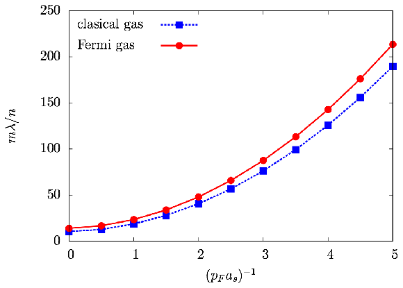
Figure 2: Scattering length dependence of the shear viscosity (left panel) and heat conductivity (right panel) at the Fermi temperature, T=TFT=T_{F}. The blue square and red circle indicate the classical Boltzmann gas and Fermi gas, respectively.
Refer to caption
Figure 3: Scattering length dependence of the quantum statistical effects for the shear viscosity (red square), heat conductivity (blue circle), the viscous relaxation times of the stress tensor (green triangle), and that of the heat conductivity (purple rhombus) are respectively shown at the Fermi temperature.
Refer to caption
Refer to caption
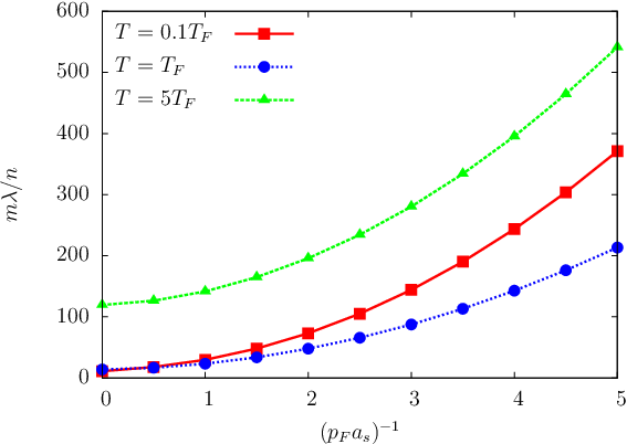
Figure 4: Scattering length dependence of the shear viscosity (left panel) and heat conductivity (right panel). The red square, blue circle, and green triangle correspond to the Fermi gas with the temperature T/TF=0.1, 1, 5T/T_{F}=0.1,\ 1,\ 5, respectively.

First, we calculate the shear viscosity and heat conductivity with varying the scattering length. The unitary limit is taken by as→∞a_{s}\to\infty, i.e., (pF​as)−1=0(p_{F}a_{s})^{-1}=0, where pFp_{F} is the Fermi momentum. For the classical Boltzmann gas, we set a=0a=0 in Eq. (2) and the corresponding equilibrium distribution function reads feqp=e−(|𝜹𝒑|2/2m−μTF)/Tf^{\mathrm{eq}}_{p}=\mathrm{e}^{-(|\boldsymbol{\delta p}|^{2}/2m-\mu_{\mathrm{TF}})/T}. For the Fermi gas, we take into account the quantum statistics by setting a=−1a=-1, and the equilibrium distribution function is fpeq=[e(|𝜹​𝒑|2/2​m−μTF)/T+1]−1f^{\mathrm{eq}}_{p}=[\mathrm{e}^{(|\boldsymbol{\delta p}|^{2}/2m-\mu_{\mathrm{TF}})/T}+1]^{-1}. The resultant data show that, as the scattering length increases, the viscous effects decrease (Fig. 2), and the quantum statistical effects increase (Fig. 3). The scattering-length dependence of the quantum statistical effects indicates that the quantum nature becomes apparent at unitarity, where the atomic gases are strongly correlated. We also see that the shear viscosity and heat conductivity decrease as the scattering length becomes smaller and they are smallest at the unitary limit for any temperature (Fig. 4).

Refer to caption
Refer to caption
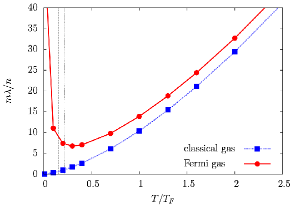
Figure 5: Temperature dependence of the shear viscosity (left panel) and heat conductivity (right panel) at the unitarity, (pF​as)−1=0(p_{F}a_{s})^{-1}=0. The blue square and red circle indicate the first-order transport coefficients of classical Boltzmann gas and the Fermi gas, respectively. The black dashed and dotted lines show the superfluid-transition temperature Tc≃0.15​TFT_{c}\simeq 0.15T_{F} and the pairing-formation temperature T∗≃0.22​TFT^{*}\simeq 0.22T_{F}, respectively.

Figure 5 shows the temperature dependence of η/n\eta/n and m​λ/nm\lambda/n. The quantum statistical effect increases the η/n\eta/n and m​λ/nm\lambda/n. The difference between the classical gas and the Fermi gas becomes larger as temperature decreases. In particular, at the temperature T<TFT<T_{F}, the differences become clear and those of the Fermi gases diverge. Three comments are in order here. (i) The quantum statistical effect is not negligible even above T∗T^{*}, below which pairing effects dominate and our computation becomes invalid. (ii) The increases of the shear viscosity and heat conductivity for the Fermi gas at small temperature are naturally understood in terms of the Pauli blocking effect; a good Fermi sphere is formed at low temperature and thus the elastic scattering rate other than the forward one is so greatly suppressed due to the Pauli blocking that the energy and momentum transport become quite efficient, which implies the increase of the shear viscosity and heat conductivity. (iii) Our result of the shear viscosity might implies that the kinetic approach is unreliable near the unitarity at low temperature even above the T∗T^{*}, in contrast to the previous works which claim good agreement between experimental results and theoretical results based on the Boltzmann equation without quantum Fermi statistics as low as 0.3​TF0.3T_{F} at unitarity.

The viscous relaxation times exhibits similar behaviors as the first-order transport coefficients. The differences between the classical gas and the Fermi gas increase at low temperature and near unitarity (see Fig. 6 and 7).

Refer to caption
Refer to caption
Figure 6: Scattering length dependence of the viscous relaxation times of the stress tensor (left panel) and heat flow (right panel) at the Fermi temperature, T=TFT=T_{F}. The blue square and red circle indicate the viscous relaxation times of classical Boltzmann gas and the Fermi gas which evaluated without the RTA, while the purple triangle and green rhombus indicate those evaluated with the RTA given by Eqs. (99) and (100). The black dashed and dotted lines show TcT_{c} and T∗T^{*}, respectively.
Refer to caption
Refer to caption
Figure 7: Temperature dependence of the viscous relaxation times of the stress tensor (left panel) and heat flow (right panel) at the unitarity, (pF​as)−1=0(p_{F}a_{s})^{-1}=0. The blue square and red circle indicate the viscous relaxation times of classical Boltzmann gas and the Fermi gas which evaluated without the RTA, while the purple triangle and green rhombus indicate those evaluated with the RTA given by Eqs. (99) and (100). The black dashed and dotted lines show TcT_{c} and T∗T^{*}, respectively.
Refer to caption
Figure 8: Temperature dependence of the viscous relaxation times of the stress tensor and heat flow of the unitary Fermi gas. The red square and blue circle respectively indicate the viscous relaxation times of the stress tensor and heat conductivity which evaluated without the RTA, while the green triangle and purple rhombus indicate those evaluated with the RTA given by Eqs. (99) and (100). The black dashed and dotted lines show TcT_{c} and T∗T^{*}, respectively.
Refer to caption
Figure 9: Temperature dependence of the error caused by the RTA are shown for the shear viscosity (red square), heat conductivity (blue circle), the viscous relaxation times of the stress tensor (green triangle), and that of the heat conductivity (purple rhombus) are respectively shown at unitarity. The black dashed and dotted lines show TcT_{c} and T∗T^{*}, respectively.

V.2 Reliability of the relaxation-time approximation

In the RTA, the collision integral in Eq. (2) is replaced by

C​[f]p=−fp−fpeqτ,\displaystyle C[f]_{p}=-\frac{f_{p}-f^{\mathrm{eq}}_{p}}{\tau}, (96)

where τ\tau is a free parameter which determines the time scale for a non-equilibrium system to relax toward the equilibrium states. Under the approximation, the shear viscosity and heat conductivity are calculated to be [19, 20, 21]

ηRTA=τ​P,λRTA=τ12​m​T​(7​Q−75​P2n),\displaystyle\eta^{\mathrm{RTA}}=\tau P,\ \ \ \lambda^{\mathrm{RTA}}=\frac{\tau}{12mT}\left(7Q-\frac{75P^{2}}{n}\right), (97)

where QQ is defined by Q≡∫pδ​v2​δ​p2​fpeqQ\equiv\int_{p}\delta v^{2}\delta p^{2}f^{\mathrm{eq}}_{p}. In addition, it should be noted that the viscous relaxation times are given by τ\tau,

τπRTA=τJRTA=τ.\displaystyle\tau^{\mathrm{RTA}}_{\pi}=\tau^{\mathrm{RTA}}_{J}=\tau. (98)

In the RTA, the relaxation-time scales of the system is characterized by only one parameter τ\tau, which must be determined phenomenologically or based on more elaborated microscopic analyses. However, the viscous relaxation times of the stress tensor and heat conductivity given by Eqs. (57) and (58) take the considerably different values (Fig. 8). This results are clearly contradict to Eq. (98) and indicate that the RTA should be modified so as to incorporate the multiple relaxation-time scales. To this end, we determine the viscous relaxation times independently with the help of the relations Eq. (97) derived from the RTA and exact value of the shear viscosity and heat conductivity as follows: We evaluate the viscous relaxation time of the stress tensor by

τ=ηexactP≡τ~πRTA,\displaystyle\tau=\frac{\eta^{\mathrm{exact}}}{P}\equiv\tilde{\tau}_{\pi}^{\mathrm{RTA}}, (99)

While the viscous relaxation time of the heat conductivity is evaluated as

τ=12​m​T​λexact(7​Q−75​P2/n)≡τ~πRTA.\displaystyle\tau=\frac{12mT\lambda^{\mathrm{exact}}}{(7Q-75P^{2}/n)}\equiv\tilde{\tau}_{\pi}^{\mathrm{RTA}}. (100)

We note that ηexact\eta^{\mathrm{exact}}, λexact\lambda^{\mathrm{exact}}, τπexact\tau^{\mathrm{exact}}_{\pi}, and τJexact\tau^{\mathrm{exact}}_{J} denote the transport coefficients and viscous relaxation times, which are respectively calculated from Eqs. (55)-(58) in an exact manner, as in the analyses in the last subsection. In Fig. 6 and 7, we compare the viscous relaxation times with and without the RTA and the numerical results of Eqs. (99) and (100) actually behave similarly compared with the exact ones qualitatively. It is remarkable that ηexact/P\eta^{\mathrm{exact}}/P well reproduces the viscous relaxation time of the stress tensor τπexact\tau^{\mathrm{exact}}_{\pi} for both the classical gas and the Fermi gas regardless of temperature and scattering length. On the other hand, the RTA still has the quantitative error and always underestimates the viscous relaxation time of the heat conductivity compared with those evaluated exactly. It is noteworthy that the error of τJ\tau_{J} caused by the RTA for the Fermi gas decreases at low temperature in contrast to that for classical gas, which is independent of temperature (Fig. 9). This behavior may be understood as follows: The RTA is a kind of the linear approximation of the collision integral with respect to the deviation of the distribution function from the equilibrium one. The deviation is attributed to the excitations of quasi-particles due to the nonequilibrium process and decreases in the cold fermionic gases since the Pauli-blocking effect suppresses the excitation of the quasi-particles inside the Fermi sphere. Therefore the linear approximation work well and the RTA reproduces the exact value of the viscous relaxation time of the heat conductivity.

It is noted that the expressions (99) and (100) derived with the RTA can be obtained by a closure approximation

⟨π^i​j,L−2​π^i​j⟩→⟨π^i​j,L−1​π^i​j⟩​⟨π^i​j,L−1​π^i​j⟩/⟨π^i​j,π^i​j⟩,\displaystyle\langle\hat{\pi}^{ij},L^{-2}\hat{\pi}^{ij}\rangle\to\langle\hat{\pi}^{ij},L^{-1}\hat{\pi}^{ij}\rangle\langle\hat{\pi}^{ij},L^{-1}\hat{\pi}^{ij}\rangle/\langle\hat{\pi}^{ij},\hat{\pi}^{ij}\rangle, (101)

in the exact expressions given by Eqs. (57) and (58). Such a closure approximation is reminiscent of the mean-field (or Hartree) approximation, and it may imply that the RTA might be validated if the vector space L​π^i​jL\hat{\pi}^{ij} is saturated by π^i​j\hat{\pi}^{ij}. Equation (99) is verified by noticing ⟨π^i​j,π^i​j⟩=10​T​P\langle\hat{\pi}^{ij},\hat{\pi}^{ij}\rangle=10TP and ⟨π^i​j,L−1​π^i​j⟩=10​T​ηexact\langle\hat{\pi}^{ij},L^{-1}\hat{\pi}^{ij}\rangle=10T\eta^{\mathrm{exact}} from Eq. (55). Then by applying the replacement (101) to Eq. (57), we obtain Eq. (99) as,

τπ=110​T​ηexact​⟨π^i​j,L−2​π^i​j⟩\displaystyle\tau_{\pi}=\frac{1}{10T\eta^{\mathrm{exact}}}\langle\hat{\pi}^{ij},L^{-2}\hat{\pi}^{ij}\rangle
→τ~πRTA=110​T​ηexact​⟨π^i​j,L−1​π^i​j⟩​⟨π^i​j,L−1​π^i​j⟩⟨π^i​j,π^i​j⟩=ηexactP.\displaystyle\to\tilde{\tau}^{\mathrm{RTA}}_{\pi}=\frac{1}{10T\eta^{\mathrm{exact}}}\frac{\langle\hat{\pi}^{ij},L^{-1}\hat{\pi}^{ij}\rangle\langle\hat{\pi}^{ij},L^{-1}\hat{\pi}^{ij}\rangle}{\langle\hat{\pi}^{ij},\hat{\pi}^{ij}\rangle}=\frac{\eta^{\mathrm{exact}}}{P}. (102)

Eq. (100) is also verified in an analogous way.

V.3 Convergence properties of the numerical results

Refer to caption
Refer to caption
Refer to caption
Refer to caption
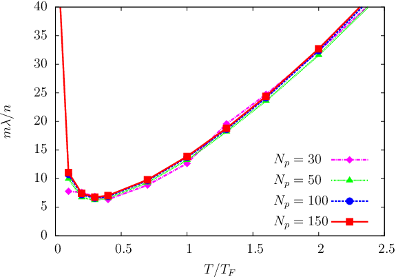
Figure 10: Temperature dependence of the shear viscosity (left top panel), heat conductivity (right top panel) and viscous relaxation times of the stress tensor (left bottom panel) and heat flow (right bottom panel) at the unitarity. Quantum Fermi statistics is taken into account in these figures. NpN_{p} is a number of meshes for the discretized momentum space and the purple rhombus, green triangle, the blue circle and red square indicate Np=30, 50, 100, 150N_{p}=30,\ 50,\ 100,\ 150, respectively.

We show that the numerical results of shear viscosity, heat conductivity, and viscous relaxation times of the stress tensor and heat flow, are well convergent. In Fig. 10, NpN_{p} is a number of meshes for the discretized momentum space. We have confirmed that the temperature dependences of all the quantities shown here are well convergent with Np=150N_{p}=150. In this confirmation, momentum upper cutoff are taken as large enough for the numerical results not to depend on them. We have also checked their scattering dependence and they are well convergent as well.

VI Conclusion

In this paper, we have derived the second-order hydrodynamic equation for non-relativistic systems with the microscopic expressions of all the transport coefficients including the viscous relaxation times by applying the RG method: It is notable that the shear viscosity and heat conductivity have the same expressions as those by the Chapman-Enskog method, and the viscous relaxation times take new but natural forms. Though the inclusion of the quantum statistical effects do not change the form of the hydrodynamic equation, it makes the microscopic expressions of the transport coefficients different, which gives the remarkable differences in the value of the transport coefficients.

By using the transport coefficients that we have obtained, we have calculated in a full numerical way the shear viscosity, heat conductivity and viscous relaxation times of the stress tensor and heat flow. Any approximation has not been used in the numerical evaluation of these quantities in the present work, which has given the exact values based on the Boltzmann equation, and the numerical convergence is readily confirmed. We have found that the Fermi statistics makes significant contributions to the first-order transport coefficients and viscous relaxation times at low temperature or small scattering length due to the Pauli blocking in the rigid Fermi sphere, which suppresses the collision rate and results in highly viscous systems. Furthermore, by using the numerical results we have examined the reliability of the relations τπ=η/P\tau_{\pi}=\eta/P and τJ=12​m​T​λ/(7​Q−75​P2/n)\tau_{J}=12mT\lambda/(7Q-75P^{2}/n), which are derived with recourse to the RTA and used rather extensively. The resulting data have shown that the ratio of the shear viscosity and pressure well agrees with the viscous relaxation time. This agreement is consistent with Ref. [47] and suggest the reliability of the RG method. Furthermore, the results encourage us to use the relation τπ=η/P\tau_{\pi}=\eta/P, which greatly simplifies the evaluation of the viscous relaxation time of the stress tensor. On the other hand, the latter relation for the viscous relaxation time does not appear to be reliable. Thus, we should use the value evaluated by Eqs. (57) and (58) instead of Eq. (97) for the viscous relaxation time of the heat conductivity, and also need to investigate the time evolution of fluids with these transport coefficients inserted in order to examine how quantitatively significant the difference of τJ\tau_{J} evaluated with and without the RTA is.

The numerical evaluation of the other transport coefficients are left as a future work. Then, we may apply the obtained second-order hydrodynamic equation to the analysis of the time evolution of the ultracold atomic gases. Furthermore, we should take account of systems with phase transitions. In particular, the behavior of the transport coefficients near the critical region and investigation of how they affect on the time-evolution of fluids are interesting.

Acknowledgment

Y.K. is supported by the Grants-in-Aid for JSPS fellows (No.15J01626). T.K. was partially supported by a Grant-in-Aid for Scientific Research from the Ministry of Education, Culture, Sports, Science and Technology (MEXT) of Japan (Nos. 20540265 and 23340067), by the Yukawa International Program for Quark-Hadron Sciences.

Appendix A Determination of the initial condition of the first-order perturbative equation

In this appendix, we present a detailed calculation of Eq. (36). F0​pF_{0p} given in Eq. (21) is calculated as

F0​p\displaystyle F_{0p} =−(fpeqf¯peq)−1(𝒗⋅∇+𝑭⋅∇p)f~p(i)\displaystyle=-(f^{\mathrm{eq}}_{p}\bar{f}^{\mathrm{eq}}_{p})^{-1}\left(\boldsymbol{v}\cdot\boldsymbol{\nabla}+\boldsymbol{F}\cdot\boldsymbol{\nabla}_{p}\right)\tilde{f}^{(i)}_{p}
=−vi​∇iTT2​(|𝜹​𝒑|22​m−μT​F)−1T​vi​δ​pj​∇iuj−vi​∇iμT​FT+Fi​δ​pim​T.\displaystyle=-v^{i}\frac{\nabla^{i}T}{T^{2}}\left(\frac{|\boldsymbol{\delta p}|^{2}}{2m}-\mu_{TF}\right)-\frac{1}{T}v^{i}\delta p^{j}\nabla^{i}u^{j}-v^{i}\frac{\nabla^{i}\mu_{TF}}{T}+F^{i}\frac{\delta p^{i}}{mT}. (1)

Then, we can calculate the projection of F0F_{0} onto the Q0-space as

[Q0​F0]p\displaystyle[Q_{0}F_{0}]_{p} =[F0−P0​F0]p=F0​p−∑α=04φ0​pαcα​⟨φ0α,F0⟩=−σi​jT​π^pi​j−∇iTT2​J^pi,\displaystyle=[F_{0}-P_{0}F_{0}]_{p}=F_{0p}-\sum_{\alpha=0}^{4}\frac{\varphi^{\alpha}_{0p}}{c^{\alpha}}\langle\varphi_{0}^{\alpha},F_{0}\rangle=-\frac{\sigma^{ij}}{T}\hat{\pi}^{ij}_{p}-\frac{\nabla^{i}T}{T^{2}}\hat{J}^{i}_{p}, (2)

where we have used the definitions of the projection operators (33) in the first equality and (32) in the second equality. Then, we arrive at Eq. (36) ,

[L−1​Q0​F0]p=−σi​jT​[L−1​π^i​j]p−∇iTT2​[L−1​J^i]p.\displaystyle[L^{-1}Q_{0}F_{0}]_{p}=-\frac{\sigma^{ij}}{T}[L^{-1}\hat{\pi}^{ij}]_{p}-\frac{\nabla^{i}T}{T^{2}}[L^{-1}\hat{J}^{i}]_{p}. (3)

Appendix B Detailed derivation of relaxation equation

We show a detailed derivation of the relaxation equation and give the explicit expressions of all the coefficients appearing in it. To this end, we reduce Eq. (49) into the relaxation equation. Using the vector notations

ψ^pα\displaystyle\hat{\psi}^{\alpha}_{p} ={π^pi​j,J^pi},\displaystyle=\{\hat{\pi}^{ij}_{p},\hat{J}^{i}_{p}\}, (1)
χ^pα\displaystyle\hat{\chi}^{\alpha}_{p} ={π^pi​j2​T​η,J^piT2​λ},\displaystyle=\left\{\frac{\hat{\pi}^{ij}_{p}}{2T\eta},\frac{\hat{J}^{i}_{p}}{T^{2}\lambda}\right\}, (2)
ψα\displaystyle\psi^{\alpha} ={πi​j,Ji},\displaystyle=\{\pi^{ij},J^{i}\}, (3)
Xα\displaystyle X^{\alpha} ={2​η​σi​j,λ​∇iT},\displaystyle=\left\{2\eta\sigma^{ij},\lambda\nabla^{i}T\right\}, (4)

with which we can write as Ψ=L−1​χ^α​ψα\Psi=L^{-1}\hat{\chi}^{\alpha}\psi^{\alpha} and Q0​F0=−χ^1α​XαQ_{0}F_{0}=-\hat{\chi}^{\alpha}_{1}X^{\alpha}. Equation (49) can be converted into the following form

ϵ⁡⟨L−1​ψ^α,χ^β⟩​ψβ\displaystyle\epsilon\langle L^{-1}\hat{\psi}^{\alpha},\hat{\chi}^{\beta}\rangle\psi^{\beta}
=ϵ⁡⟨L−1​ψ^α,χ^β⟩​Xβ+⟨L−1​ψ^α,L−1​χ^β⟩​DD​t​ψβ+ϵ⁡⟨L−1​ψ^α,δ​Ki​L−1​χ^β⟩​∇iψβ\displaystyle=\epsilon\langle L^{-1}\hat{\psi}^{\alpha},\hat{\chi}^{\beta}\rangle X^{\beta}+\langle L^{-1}\hat{\psi}^{\alpha},L^{-1}\hat{\chi}^{\beta}\rangle\frac{\mathrm{D}}{\mathrm{D}t}\psi^{\beta}+\epsilon\langle L^{-1}\hat{\psi}^{\alpha},\delta K^{i}L^{-1}\hat{\chi}^{\beta}\rangle\nabla^{i}\psi^{\beta}
+ϵ⟨L−1ψ^α,feqf¯eq(DD​t+ϵ𝜹𝑲⋅∇+ϵ𝑭⋅∇K)feqf¯eqL−1χ^β⟩ψβ\displaystyle+\epsilon\Big<L^{-1}\hat{\psi}^{\alpha},f^{\mathrm{eq}}\bar{f}^{\mathrm{eq}}\left(\frac{\mathrm{D}}{\mathrm{D}t}+\epsilon\boldsymbol{\delta K}\cdot\boldsymbol{\nabla}+\epsilon\boldsymbol{F}\cdot\boldsymbol{\nabla}_{K}\right)f^{\mathrm{eq}}\bar{f}^{\mathrm{eq}}L^{-1}\hat{\chi}^{\beta}\Big>\psi^{\beta}
−ϵ2​12​⟨L−1​ψ^α,B⁡[L−1​χ^1β,L−1​χ^γ]⟩​ψβ​ψγ,\displaystyle-\epsilon^{2}\frac{1}{2}\langle L^{-1}\hat{\psi}^{\alpha},B[L^{-1}\hat{\chi}^{\beta}_{1},L^{-1}\hat{\chi}^{\gamma}]\rangle\psi^{\beta}\psi^{\gamma}, (5)

where we have defined [δ​Ki]p≡δ​pi/m=δ​vi[\delta K^{i}]_{p}\equiv\delta p^{i}/m=\delta v^{i} and [∇Ki]p≡∇pi[\nabla_{K}^{i}]_{p}\equiv\nabla_{p}^{i}.

The coefficients of the first, third, and fourth terms in the right-hand side of Eq. (5) can be written as

⟨L−1ψ^α,ψ^β⟩=(−2​T​η​Δi​j​k​l00−T2​λ​Δi​j),\displaystyle\big<L^{-1}\hat{\psi}^{\alpha},\hat{\psi}^{\beta}\big>=\begin{pmatrix}-2T\eta\Delta^{ijkl}&0\\ 0&-T^{2}\lambda\Delta^{ij}\end{pmatrix}, (6)
⟨L−1ψ^α,L−1ψ^β⟩=(2​T​η​τπ​Δi​j​k​l00T2​λ​τJ​Δi​j),\displaystyle\big<L^{-1}\hat{\psi}^{\alpha},L^{-1}\hat{\psi}^{\beta}\big>=\begin{pmatrix}2T\eta\tau_{\pi}\Delta^{ijkl}&0\\ 0&T^{2}\lambda\tau_{J}\Delta^{ij}\\ \end{pmatrix}, (7)
⟨L−1ψ^α,δKmL−1ψ^β⟩=(0T2​λ​ℓπ​J​Δi​j​k​l2​T​η​ℓJ​π​Δi​j​k​l0),\displaystyle\big<L^{-1}\hat{\psi}^{\alpha},\delta K^{m}L^{-1}\hat{\psi}^{\beta}\big>=\begin{pmatrix}0&T^{2}\lambda\ell_{\pi J}\Delta^{ijkl}\\ 2T\eta\ell_{J\pi}\Delta^{ijkl}&0\\ \end{pmatrix}, (8)

where transport coefficients introduced here are defined as follows:

τπ≡110​T​η⟨π^i​j,L−2​π^i​j⟩,\displaystyle\tau_{\pi}\equiv\frac{1}{10T\eta}\big<\hat{\pi}^{ij},L^{-2}\hat{\pi}^{ij}\big>, (9)
τJ≡13​T2​λ⟨J^i,L−2​J^i⟩,\displaystyle\tau_{J}\equiv\frac{1}{3T^{2}\lambda}\big<\hat{J}^{i},L^{-2}\hat{J}^{i}\big>, (10)

which are viscous relaxation times for the stress tensor and heat flow, respectively, and

ℓπ​J≡15​T2​λ⟨L−1​π^i​j,δ​Ki​L−1​J^j⟩,\displaystyle\ell_{\pi J}\equiv\frac{1}{5T^{2}\lambda}\big<L^{-1}\hat{\pi}^{ij},\delta K^{i}L^{-1}\hat{J}^{j}\big>, (11)
ℓJ​π≡110​T​η⟨L−1​J^i,δ​Kj​L−1​π^i​j⟩,\displaystyle\ell_{J\pi}\equiv\frac{1}{10T\eta}\big<L^{-1}\hat{J}^{i},\delta K^{j}L^{-1}\hat{\pi}^{ij}\big>, (12)

which are so called viscous relaxation lengths.

Then, let us rewrite the last term in the right-hand side of Eq. (5) as

ϵ22⟨L−1π^i​j,B[L−1χ^β][L−1χ^γ]⟩ψβψγ=bπ​π​ππm⟨kπl⟩m+bπ​J​JJ⟨kJl⟩,\displaystyle\frac{\epsilon^{2}}{2}\big<L^{-1}\hat{\pi}^{ij},B[L^{-1}\hat{\chi}^{\beta}][L^{-1}\hat{\chi}^{\gamma}]\big>\psi^{\beta}\psi^{\gamma}=b_{\pi\pi\pi}\pi^{m\langle k}\pi^{l\rangle m}+b_{\pi JJ}J^{\langle k}J^{l\rangle}, (13)
ϵ22⟨L−1​J^i,B⁡[L−1​χ^β]​[L−1​χ^γ]⟩ψβ​ψγ=bJ​π​J​πi​j​Jj,\displaystyle\frac{\epsilon^{2}}{2}\big<L^{-1}\hat{J}^{i},B[L^{-1}\hat{\chi}^{\beta}][L^{-1}\hat{\chi}^{\gamma}]\big>\psi^{\beta}\psi^{\gamma}=b_{J\pi J}\pi^{ij}J^{j}, (14)

where the transport coefficients are defined by

bπ​π​π≡370​T2​η2⟨L−1​π^i​j,B⁡[L−1​π^i​k]​[L−1​π^j​k]⟩,\displaystyle b_{\pi\pi\pi}\equiv\frac{3}{70T^{2}\eta^{2}}\big<L^{-1}\hat{\pi}^{ij},B[L^{-1}\hat{\pi}^{ik}][L^{-1}\hat{\pi}^{jk}]\big>, (15)
bπ​J​J≡110​T4​λ2⟨L−1​π^i​j,B⁡[L−1​J^i]​[L−1​J^j]⟩,\displaystyle b_{\pi JJ}\equiv\frac{1}{10T^{4}\lambda^{2}}\big<L^{-1}\hat{\pi}^{ij},B[L^{-1}\hat{J}^{i}][L^{-1}\hat{J}^{j}]\big>, (16)
bJ​J​π≡110​T3​η​λ⟨L−1​J^i,B⁡[L−1​J^j]​[L−1​π^i​j]⟩.\displaystyle b_{JJ\pi}\equiv\frac{1}{10T^{3}\eta\lambda}\big<L^{-1}\hat{J}^{i},B[L^{-1}\hat{J}^{j}][L^{-1}\hat{\pi}^{ij}]\big>. (17)

We consider the forth term in the right-hand side of Eq. (5):

ϵ⟨L−1ψ^α,(feqf¯eq)−1[DD​t+ϵ𝜹𝑲⋅∇+ϵ𝑭⋅∇K]feqf¯eqL−1χ^β⟩ψ^β\displaystyle\epsilon\Big<L^{-1}\hat{\psi}^{\alpha},(f^{\mathrm{eq}}\bar{f}^{\mathrm{eq}})^{-1}\left[\frac{\mathrm{D}}{\mathrm{D}t}+\epsilon\boldsymbol{\delta K}\cdot\boldsymbol{\nabla}+\epsilon\boldsymbol{F}\cdot\boldsymbol{\nabla}_{K}\right]f^{\mathrm{eq}}\bar{f}^{\mathrm{eq}}L^{-1}\hat{\chi}^{\beta}\Big>\hat{\psi}^{\beta}
=ϵ⟨L−1​ψ^α,(feq​f¯eq)−1​∂∂T​[feq​f¯eq​L−1​χ^β]⟩ψ^β​D​TD​t\displaystyle=\epsilon\Big<L^{-1}\hat{\psi}^{\alpha},(f^{\mathrm{eq}}\bar{f}^{\mathrm{eq}})^{-1}\frac{\partial}{\partial T}[f^{\mathrm{eq}}\bar{f}^{\mathrm{eq}}L^{-1}\hat{\chi}^{\beta}]\Big>\hat{\psi}^{\beta}\frac{\mathrm{D}T}{\mathrm{D}t}
+ϵ2⟨L−1​ψ^α,(feq​f¯eq)−1​δ​Ka​∂∂T​[feq​f¯eq​L−1​χ^β]⟩ψ^β​∇aT\displaystyle+\epsilon^{2}\Big<L^{-1}\hat{\psi}^{\alpha},(f^{\mathrm{eq}}\bar{f}^{\mathrm{eq}})^{-1}\delta K^{a}\frac{\partial}{\partial T}[f^{\mathrm{eq}}\bar{f}^{\mathrm{eq}}L^{-1}\hat{\chi}^{\beta}]\Big>\hat{\psi}^{\beta}\nabla^{a}T
+ϵ⟨L−1ψ^α,(feqf¯eq)−1∂∂μT​F[feqf¯eqL−1χ^β⟩ψ^βD​μT​FD​t\displaystyle+\epsilon\Big<L^{-1}\hat{\psi}^{\alpha},(f^{\mathrm{eq}}\bar{f}^{\mathrm{eq}})^{-1}\frac{\partial}{\partial\mu_{TF}}[f^{\mathrm{eq}}\bar{f}^{\mathrm{eq}}L^{-1}\hat{\chi}^{\beta}\Big>\hat{\psi}^{\beta}\frac{\mathrm{D}\mu_{TF}}{\mathrm{D}t}
+ϵ2⟨L−1​ψ^α,(feq​f¯eq)−1​δ​Ka​∂∂μT​F​[feq​feq​L−1​χ^β]⟩ψ^β​∇aμT​F\displaystyle+\epsilon^{2}\Big<L^{-1}\hat{\psi}^{\alpha},(f^{\mathrm{eq}}\bar{f}^{\mathrm{eq}})^{-1}\delta K^{a}\frac{\partial}{\partial\mu_{TF}}[f^{\mathrm{eq}}f^{\mathrm{eq}}L^{-1}\hat{\chi}^{\beta}]\Big>\hat{\psi}^{\beta}\nabla^{a}\mu_{TF}
+ϵ⟨L−1​ψ^α,(feq​f¯eq)−1​∂∂ub​[feq​feq​L−1​χ^β]⟩ψ^β​D​ubD​t\displaystyle+\epsilon\Big<L^{-1}\hat{\psi}^{\alpha},(f^{\mathrm{eq}}\bar{f}^{\mathrm{eq}})^{-1}\frac{\partial}{\partial u^{b}}[f^{\mathrm{eq}}f^{\mathrm{eq}}L^{-1}\hat{\chi}^{\beta}]\Big>\hat{\psi}^{\beta}\frac{\mathrm{D}u^{b}}{\mathrm{D}t}
+ϵ2⟨L−1​ψ^α,(feq​f¯eq)−1​δ​Ka​∂∂ub​[feq​feq​L−1​χ^β]⟩ψ^β​∇aub\displaystyle+\epsilon^{2}\Big<L^{-1}\hat{\psi}^{\alpha},(f^{\mathrm{eq}}\bar{f}^{\mathrm{eq}})^{-1}\delta K^{a}\frac{\partial}{\partial u^{b}}[f^{\mathrm{eq}}f^{\mathrm{eq}}L^{-1}\hat{\chi}^{\beta}]\Big>\hat{\psi}^{\beta}\nabla^{a}u^{b}
+ϵ2⟨L−1​ψ^α,(feq​f¯eq)−1​∇Ka[feq​feq​L−1​χ^β]⟩ψ^β​Fam.\displaystyle+\epsilon^{2}\Big<L^{-1}\hat{\psi}^{\alpha},(f^{\mathrm{eq}}\bar{f}^{\mathrm{eq}})^{-1}\nabla_{K}^{a}[f^{\mathrm{eq}}f^{\mathrm{eq}}L^{-1}\hat{\chi}^{\beta}]\Big>\hat{\psi}^{\beta}\frac{F^{a}}{m}. (18)

The Lagrange derivative of TT, μT​F\mu_{TF}, and ubu^{b} are rewritten by using the balance equation up to the first order with respect to ε\varepsilon, which corresponds to the Euler’s equation:

D​TD​t\displaystyle\frac{\mathrm{D}T}{\mathrm{D}t} =−ϵ2​T3∇⋅𝒖+𝒪(ϵ2),\displaystyle=-\epsilon\frac{2T}{3}\boldsymbol{\nabla}\cdot\boldsymbol{u}+\mathcal{O}(\epsilon^{2}), (19)
D​μT​FD​t\displaystyle\frac{\mathrm{D}\mu_{TF}}{\mathrm{D}t} =−ϵ2​μT​F3∇⋅𝒖+𝒪(ϵ2),\displaystyle=-\epsilon\frac{2\mu_{TF}}{3}\boldsymbol{\nabla}\cdot\boldsymbol{u}+\mathcal{O}(\epsilon^{2}), (20)
D​ubD​t\displaystyle\frac{\mathrm{D}u^{b}}{\mathrm{D}t} =−ϵ​∇iP+ϵ​n​Fi+𝒪⁡(ϵ2),\displaystyle=-\epsilon\nabla^{i}P+\epsilon nF^{i}+\mathcal{O}(\epsilon^{2}), (21)

where we have used the relation d​n=(∂n/∂T)​d​T+(∂n/∂μT​F)​d​μT​F\mathrm{d}n=(\partial n/\partial T)\mathrm{d}T+(\partial n/\partial\mu_{TF})\mathrm{d}\mu_{TF} in the derivation of Eq. (20). Then, Eq. (18) takes the following forms

ϵ⟨L−1π^i​j,(feqf¯eq)−1[DD​t+ϵ𝜹𝑲⋅∇+ϵ𝑭⋅∇K]feqf¯eqχ^β⟩ψβ\displaystyle\epsilon\Big<L^{-1}\hat{\pi}^{ij},(f^{\mathrm{eq}}\bar{f}^{\mathrm{eq}})^{-1}\left[\frac{\mathrm{D}}{\mathrm{D}t}+\epsilon\boldsymbol{\delta K}\cdot\boldsymbol{\nabla}+\epsilon\boldsymbol{F}\cdot\boldsymbol{\nabla}_{K}\right]f^{\mathrm{eq}}\bar{f}^{\mathrm{eq}}\hat{\chi}^{\beta}\Big>\psi^{\beta}
=−ϵ2(κπ​π(1)πi​j∇⋅𝒖+κπ​π(2)πk⟨iσj⟩k+κπ​π(3)πk⟨iωj⟩k+κπ​J(1)J⟨i∇j⟩n+κπ​J(2)J⟨i∇j⟩P+κπ​J(3)J⟨iFj⟩),\displaystyle=-\epsilon^{2}\left(\kappa_{\pi\pi}^{(1)}\pi^{ij}\boldsymbol{\nabla}\cdot\boldsymbol{u}+\kappa_{\pi\pi}^{(2)}\pi^{k\langle i}\sigma^{j\rangle k}+\kappa_{\pi\pi}^{(3)}\pi^{k\langle i}\omega^{j\rangle k}+\kappa_{\pi J}^{(1)}J^{\langle i}\nabla^{j\rangle}n+\kappa_{\pi J}^{(2)}J^{\langle i}\nabla^{j\rangle}P+\kappa_{\pi J}^{(3)}J^{\langle i}F^{j\rangle}\right), (22)
ϵ⟨L−1J^k,(feqf¯eq)−1[DD​t+ϵ𝜹𝑲⋅∇+ϵ𝑭⋅∇K]feqf¯eqL−1χ^β⟩ψβ\displaystyle\epsilon\Big<L^{-1}\hat{J}^{k},(f^{\mathrm{eq}}\bar{f}^{\mathrm{eq}})^{-1}\left[\frac{\mathrm{D}}{\mathrm{D}t}+\epsilon\boldsymbol{\delta K}\cdot\boldsymbol{\nabla}+\epsilon\boldsymbol{F}\cdot\boldsymbol{\nabla}_{K}\right]f^{\mathrm{eq}}\bar{f}^{\mathrm{eq}}L^{-1}\hat{\chi}^{\beta}\Big>\psi^{\beta}
=−ϵ2(κJ​π(1)πi​j∇jn+κJ​π(2)πi​j∇jP+κJ​π(3)πi​jFj+κJ​J(1)Ji∇⋅𝒖+κJ​π(2)Jjσi​j+κJ​π(3)Jjωi​j),\displaystyle=-\epsilon^{2}\left(\kappa_{J\pi}^{(1)}\pi^{ij}\nabla^{j}n+\kappa_{J\pi}^{(2)}\pi^{ij}\nabla^{j}P+\kappa_{J\pi}^{(3)}\pi^{ij}F^{j}+\kappa_{JJ}^{(1)}J^{i}\boldsymbol{\nabla}\cdot\boldsymbol{u}+\kappa_{J\pi}^{(2)}J^{j}\sigma^{ij}+\kappa_{J\pi}^{(3)}J^{j}\omega^{ij}\right), (23)

where we have used ∇iuj=σi​j+ωi​j+δi​j∇⋅𝒖/3\nabla^{i}u^{j}=\sigma^{ij}+\omega^{ij}+\delta^{ij}\boldsymbol{\nabla}\cdot\boldsymbol{u}/3 with the vorticity ωi​j≡(∇iuj−∇jui)/2\omega^{ij}\equiv(\nabla^{i}u^{j}-\nabla^{j}u^{i})/2, and the transport coefficients are defined as follows:

κπ​π(1)\displaystyle\kappa_{\pi\pi}^{(1)} ≡−110⟨L−1π^i​j,(feqf¯eq)−1[−2​T3∂∂T−2​μT​F3∂∂μT​F+13δKa∂∂ua]feq​f¯eq​L−1​π^i​jT​η⟩,\displaystyle\equiv-\frac{1}{10}\Big<L^{-1}\hat{\pi}^{ij},(f^{\mathrm{eq}}\bar{f}^{\mathrm{eq}})^{-1}\left[-\frac{2T}{3}\frac{\partial}{\partial T}-\frac{2\mu_{TF}}{3}\frac{\partial}{\partial\mu_{TF}}+\frac{1}{3}\delta K^{a}\frac{\partial}{\partial u^{a}}\right]\frac{f^{\mathrm{eq}}\bar{f}^{\mathrm{eq}}L^{-1}\hat{\pi}^{ij}}{T\eta}\Big>, (24)
κπ​π(2)\displaystyle\kappa_{\pi\pi}^{(2)} ≡−635Δk​j​a​b⟨L−1π^i​j,(feqf¯eq)−1δKa∂∂ubfeq​f¯eq​L−1​π^k​iT​η⟩,\displaystyle\equiv-\frac{6}{35}\Delta^{kjab}\Big<L^{-1}\hat{\pi}^{ij},(f^{\mathrm{eq}}\bar{f}^{\mathrm{eq}})^{-1}\delta K^{a}\frac{\partial}{\partial u^{b}}\frac{f^{\mathrm{eq}}\bar{f}^{\mathrm{eq}}L^{-1}\hat{\pi}^{ki}}{T\eta}\Big>, (25)
κπ​π(3)\displaystyle\kappa_{\pi\pi}^{(3)} ≡−215Ωk​j​a​b⟨L−1π^i​j,(feqf¯eq)−1δKa∂∂ubfeq​f¯eq​L−1​π^k​iT​η⟩=−2τπ,\displaystyle\equiv-\frac{2}{15}\Omega^{kjab}\Big<L^{-1}\hat{\pi}^{ij},(f^{\mathrm{eq}}\bar{f}^{\mathrm{eq}})^{-1}\delta K^{a}\frac{\partial}{\partial u^{b}}\frac{f^{\mathrm{eq}}\bar{f}^{\mathrm{eq}}L^{-1}\hat{\pi}^{ki}}{T\eta}\Big>=-2\tau_{\pi}, (26)
κπ​J(1)\displaystyle\kappa_{\pi J}^{(1)} ≡−15⟨L−1π^i​j,(feqf¯eq)−1δKi2​T23​n​T−2​A​hT​F[∂∂T−s∂∂μT​F]feq​f¯eq​L−1​J^jT2​λ⟩,\displaystyle\equiv-\frac{1}{5}\Big<L^{-1}\hat{\pi}^{ij},(f^{\mathrm{eq}}\bar{f}^{\mathrm{eq}})^{-1}\delta K^{i}\frac{2T^{2}}{3nT-2Ah_{TF}}\left[\frac{\partial}{\partial T}-s\frac{\partial}{\partial\mu_{TF}}\right]\frac{f^{\mathrm{eq}}\bar{f}^{\mathrm{eq}}L^{-1}\hat{J}^{j}}{T^{2}\lambda}\Big>, (27)
κπ​J(2)\displaystyle\kappa_{\pi J}^{(2)} ≡−15⟨L−1​π^i​j,(feq​f¯eq)−1\displaystyle\equiv-\frac{1}{5}\Big<L^{-1}\hat{\pi}^{ij},(f^{\mathrm{eq}}\bar{f}^{\mathrm{eq}})^{-1}
×[−δ​Ki​2​A​T/n3​n​T−2​A​hT​F​∂∂T+δ​Ki​1n​∂∂μT​F−∂∂ui]​feq​f¯eq​L−1​J^jT2​λ⟩,\displaystyle\times\left[-\delta K^{i}\frac{2AT/n}{3nT-2Ah_{TF}}\frac{\partial}{\partial T}+\delta K^{i}\frac{1}{n}\frac{\partial}{\partial\mu_{TF}}-\frac{\partial}{\partial u^{i}}\right]\frac{f^{\mathrm{eq}}\bar{f}^{\mathrm{eq}}L^{-1}\hat{J}^{j}}{T^{2}\lambda}\Big>, (28)
κπ​J(3)\displaystyle\kappa_{\pi J}^{(3)} ≡−15⟨L−1π^i​j,(feqf¯eq)−1[n∂∂ui+∇Ki]feq​f¯eq​L−1​J^jT2​λ⟩,\displaystyle\equiv-\frac{1}{5}\Big<L^{-1}\hat{\pi}^{ij},(f^{\mathrm{eq}}\bar{f}^{\mathrm{eq}})^{-1}\left[n\frac{\partial}{\partial u^{i}}+\nabla_{K}^{i}\right]\frac{f^{\mathrm{eq}}\bar{f}^{\mathrm{eq}}L^{-1}\hat{J}^{j}}{T^{2}\lambda}\Big>, (29)
κJ​π(1)\displaystyle\kappa_{J\pi}^{(1)} ≡−110⟨L−1J^i,(feqf¯eq)−1δKj2​T23​n​T−2​A​hT​F[∂∂T−s∂∂μT​F]feq​f¯eq​L−1​π^i​jT​η⟩,\displaystyle\equiv-\frac{1}{10}\Big<L^{-1}\hat{J}^{i},(f^{\mathrm{eq}}\bar{f}^{\mathrm{eq}})^{-1}\delta K^{j}\frac{2T^{2}}{3nT-2Ah_{TF}}\left[\frac{\partial}{\partial T}-s\frac{\partial}{\partial\mu_{TF}}\right]\frac{f^{\mathrm{eq}}\bar{f}^{\mathrm{eq}}L^{-1}\hat{\pi}^{ij}}{T\eta}\Big>, (30)
κJ​π(2)\displaystyle\kappa_{J\pi}^{(2)} ≡−110⟨L−1​J^i,(feq​f¯eq)−1\displaystyle\equiv-\frac{1}{10}\Big<L^{-1}\hat{J}^{i},(f^{\mathrm{eq}}\bar{f}^{\mathrm{eq}})^{-1}
×[−δ​Kj​2​A​T/n3​n​T−2​A​hT​F​∂∂T+δ​Kj​1n​∂∂μT​F−∂∂uj]​feq​f¯eq​L−1​π^i​jT​η⟩,\displaystyle\times\left[-\delta K^{j}\frac{2AT/n}{3nT-2Ah_{TF}}\frac{\partial}{\partial T}+\delta K^{j}\frac{1}{n}\frac{\partial}{\partial\mu_{TF}}-\frac{\partial}{\partial u^{j}}\right]\frac{f^{\mathrm{eq}}\bar{f}^{\mathrm{eq}}L^{-1}\hat{\pi}^{ij}}{T\eta}\Big>, (31)
κJ​π(3)\displaystyle\kappa_{J\pi}^{(3)} ≡−110​T​η⟨L−1J^i,(feqf¯eq)−1[n∂∂uj+∇Kj]feq​f¯eq​L−1​π^i​jT​η⟩,\displaystyle\equiv-\frac{1}{10T\eta}\Big<L^{-1}\hat{J}^{i},(f^{\mathrm{eq}}\bar{f}^{\mathrm{eq}})^{-1}\left[n\frac{\partial}{\partial u^{j}}+\nabla_{K}^{j}\right]\frac{f^{\mathrm{eq}}\bar{f}^{\mathrm{eq}}L^{-1}\hat{\pi}^{ij}}{T\eta}\Big>, (32)
κJ​J(1)\displaystyle\kappa_{JJ}^{(1)} ≡−13⟨L−1J^i,(feqf¯eq)−1[−2​T3∂∂T−2​μT​F3∂∂μT​F+13δKa∂∂ua]feq​f¯eq​L−1​J^iT2​λ⟩,\displaystyle\equiv-\frac{1}{3}\Big<L^{-1}\hat{J}^{i},(f^{\mathrm{eq}}\bar{f}^{\mathrm{eq}})^{-1}\left[-\frac{2T}{3}\frac{\partial}{\partial T}-\frac{2\mu_{TF}}{3}\frac{\partial}{\partial\mu_{TF}}+\frac{1}{3}\delta K^{a}\frac{\partial}{\partial u^{a}}\right]\frac{f^{\mathrm{eq}}\bar{f}^{\mathrm{eq}}L^{-1}\hat{J}^{i}}{T^{2}\lambda}\Big>, (33)
κJ​J(2)\displaystyle\kappa_{JJ}^{(2)} ≡−15Δi​j​k​l⟨L−1J^i,(feqf¯eq)−1δKk∂∂ulfeq​f¯eq​L−1​J^jT2​λ⟩,\displaystyle\equiv-\frac{1}{5}\Delta^{ijkl}\Big<L^{-1}\hat{J}^{i},(f^{\mathrm{eq}}\bar{f}^{\mathrm{eq}})^{-1}\delta K^{k}\frac{\partial}{\partial u^{l}}\frac{f^{\mathrm{eq}}\bar{f}^{\mathrm{eq}}L^{-1}\hat{J}^{j}}{T^{2}\lambda}\Big>, (34)
κJ​J(3)\displaystyle\kappa_{JJ}^{(3)} ≡−13Ωi​j​k​l⟨L−1J^i,(feqf¯eq)−1δKk∂∂ulfeq​f¯eq​L−1​J^jT2​λ⟩=τJ,\displaystyle\equiv-\frac{1}{3}\Omega^{ijkl}\Big<L^{-1}\hat{J}^{i},(f^{\mathrm{eq}}\bar{f}^{\mathrm{eq}})^{-1}\delta K^{k}\frac{\partial}{\partial u^{l}}\frac{f^{\mathrm{eq}}\bar{f}^{\mathrm{eq}}L^{-1}\hat{J}^{j}}{T^{2}\lambda}\Big>=\tau_{J}, (35)

where Ωi​j​k​l≡(δi​k​δj​l−δi​l​δj​k)/2\Omega^{ijkl}\equiv(\delta^{ik}\delta^{jl}-\delta^{il}\delta^{jk})/2 is an antisymmetric projection operator, and AA is defined by A≡T​∂n/∂μTFA\equiv T\partial n/\partial\mu_{\mathrm{TF}}.

Here, we show that κπ​π(3)=−2​τπ\kappa_{\pi\pi}^{(3)}=-2\tau_{\pi} by analytically evaluating the inner product of Eq. (26). Without loss of generality, L−1​π^μ​νL^{-1}\hat{\pi}^{\mu\nu} may be written as

L−1​π^i​j=C⁡(|𝜹​𝑲|)​Δi​j​k​l​δ​Kk​δ​Kl.\displaystyle L^{-1}\hat{\pi}^{ij}=C(|\boldsymbol{\delta K}|)\Delta^{ijkl}\delta K^{k}\delta K^{l}. (36)

We do not need the specific form of C⁡(|𝜹​𝑲|)C(|\boldsymbol{\delta K}|) in this computation. Then κπ​π(3)\kappa_{\pi\pi}^{(3)} can be written as

κπ​π(3)=−215​Ωk​j​a​b⟨C⁡(|𝜹​𝑲|)​Δi​j​c​d​δ​Kc​δ​Kd,(feq​f¯eq)−1​δ​Ka​∂∂ub​feq​f¯eq​C​(|𝜹​𝑲|)​Δk​i​e​f​δ​Ke​δ​KfT​η⟩.\displaystyle\kappa_{\pi\pi}^{(3)}=-\frac{2}{15}\Omega^{kjab}\Big<C(|\boldsymbol{\delta K}|)\Delta^{ijcd}\delta K^{c}\delta K^{d},(f^{\mathrm{eq}}\bar{f}^{\mathrm{eq}})^{-1}\delta K^{a}\frac{\partial}{\partial u^{b}}\frac{f^{\mathrm{eq}}\bar{f}^{\mathrm{eq}}C(|\boldsymbol{\delta K}|)\Delta^{kief}\delta K^{e}\delta K^{f}}{T\eta}\Big>. (37)

Here we write down useful formulae for further conversion:

Ωk​j​a​b​δ​Ka​∂∂ub​|𝜹​𝑲|\displaystyle\Omega^{kjab}\delta K^{a}\frac{\partial}{\partial u^{b}}|\boldsymbol{\delta K}| =Ωk​j​a​b​δ​Ka​−δ​Kb|𝜹​𝑲|=0,\displaystyle=\Omega^{kjab}\delta K^{a}\frac{-\delta K^{b}}{|\boldsymbol{\delta K}|}=0, (38)
Ωk​j​a​b​Δi​j​c​d​δ​Kc​δ​Kd​δ​Ka​Δk​i​e​f​[−δb​e​δ​Kf−δb​f​δ​Ke]\displaystyle\Omega^{kjab}\Delta^{ijcd}\delta K^{c}\delta K^{d}\delta K^{a}\Delta^{kief}[-\delta^{be}\delta K^{f}-\delta^{bf}\delta K^{e}] =32​Δi​j​k​l​δ​Ki​δ​Kj​δ​Kk​δ​Kl\displaystyle=\frac{3}{2}\Delta^{ijkl}\delta K^{i}\delta K^{j}\delta K^{k}\delta K^{l}
=32​Δi​j​k​l​δ​Kk​δ​Kl​Δi​j​a​b​δ​Ka​δ​Kb.\displaystyle=\frac{3}{2}\Delta^{ijkl}\delta K^{k}\delta K^{l}\Delta^{ijab}\delta K^{a}\delta K^{b}. (39)

By using these formulae, Eq. (37) is calculated to be

κπ​π(3)\displaystyle\kappa_{\pi\pi}^{(3)} =−215Ωk​j​a​b⟨C(|𝜹𝑲|)Δi​j​c​dδKcδKd,δKaC⁡(|𝜹​𝑲|)​Δk​i​e​f​(−δb​e​δ​Kf−δb​f​δ​Ke)T​η⟩\displaystyle=-\frac{2}{15}\Omega^{kjab}\Big<C(|\boldsymbol{\delta K}|)\Delta^{ijcd}\delta K^{c}\delta K^{d},\delta K^{a}\frac{C(|\boldsymbol{\delta K}|)\Delta^{kief}(-\delta^{be}\delta K^{f}-\delta^{bf}\delta K^{e})}{T\eta}\Big>
=−215​3/22​T​η​⟨L^−1​π^μ​ν,L^−1​π^μ​ν⟩\displaystyle=-\frac{2}{15}\frac{3/2}{2T\eta}\langle\hat{L}^{-1}\hat{\pi}^{\mu\nu},\hat{L}^{-1}\hat{\pi}_{\mu\nu}\rangle
=−2​τπ.\displaystyle=-2\tau_{\pi}. (40)

Similarly we can show that κJ​J(3)=τJ\kappa_{JJ}^{(3)}=\tau_{J} by evaluating the inner product of Eq. (35).

Combining the formulas derived so far, we can rewrite the relaxation equation Eq. (5) in the following forms:

ϵ​πi​j\displaystyle\epsilon\pi^{ij} =ϵ2ησi​j−ϵ2τπDD​tπi​j−ϵ2ℓπ​J∇⟨iJj⟩\displaystyle=\epsilon 2\eta\sigma^{ij}-\epsilon^{2}\tau_{\pi}\frac{\mathrm{D}}{\mathrm{D}t}\pi^{ij}-\epsilon^{2}\ell_{\pi J}\nabla^{\langle i}J^{j\rangle}
+ϵ2κπ​π(1)πi​j∇⋅𝒖+ϵ2κπ​π(2)πk⟨iσj⟩k−ϵ22τππk⟨ωj⟩k\displaystyle+\epsilon^{2}\kappa_{\pi\pi}^{(1)}\pi^{ij}\boldsymbol{\nabla}\cdot\boldsymbol{u}+\epsilon^{2}\kappa_{\pi\pi}^{(2)}\pi^{k\langle i}\sigma^{j\rangle k}-\epsilon^{2}2\tau_{\pi}\pi^{k\langle}\omega^{j\rangle k}
+ϵ2κπ​J(1)J⟨i∇j⟩n+ϵ2κπ​J(2)J⟨i∇j⟩P+ϵ2κπ​J(3)J⟨iFj⟩\displaystyle+\epsilon^{2}\kappa_{\pi J}^{(1)}J^{\langle i}\nabla^{j\rangle}n+\epsilon^{2}\kappa_{\pi J}^{(2)}J^{\langle i}\nabla^{j\rangle}P+\epsilon^{2}\kappa_{\pi J}^{(3)}J^{\langle i}F^{j\rangle}
+ϵ2bπ​π​ππk⟨iπj⟩k+ϵ2bπ​J​JJ⟨iJj⟩,\displaystyle+\epsilon^{2}b_{\pi\pi\pi}\pi^{k\langle i}\pi^{j\rangle k}+\epsilon^{2}b_{\pi JJ}J^{\langle i}J^{j\rangle}, (41)
ϵ​Ji\displaystyle\epsilon J^{i} =ϵ​λ​∇iT−ϵ2​τJ​DD​t​Ji−ϵ2​ℓJ​π​∇jπi​j\displaystyle=\epsilon\lambda\nabla^{i}T-\epsilon^{2}\tau_{J}\frac{\mathrm{D}}{\mathrm{D}t}J^{i}-\epsilon^{2}\ell_{J\pi}\nabla^{j}\pi^{ij}
+ϵ2​κJ​π(1)​πi​j​∇jn+ϵ2​κJ​π(2)​πi​j​∇jP+ϵ2​κJ​π(3)​πi​j​Fj\displaystyle+\epsilon^{2}\kappa_{J\pi}^{(1)}\pi^{ij}\nabla^{j}n+\epsilon^{2}\kappa_{J\pi}^{(2)}\pi^{ij}\nabla^{j}P+\epsilon^{2}\kappa_{J\pi}^{(3)}\pi^{ij}F^{j}
+ϵ2κJ​J(1)Ji∇⋅𝒖+ϵ2κJ​J(2)Jjσi​j+ϵ2τJJjωi​j\displaystyle+\epsilon^{2}\kappa_{JJ}^{(1)}J^{i}\boldsymbol{\nabla}\cdot\boldsymbol{u}+\epsilon^{2}\kappa_{JJ}^{(2)}J^{j}\sigma^{ij}+\epsilon^{2}\tau_{J}J^{j}\omega^{ij}
+ϵ2​bJ​J​π​Jj​πi​j.\displaystyle+\epsilon^{2}b_{JJ\pi}J^{j}\pi^{ij}. (42)

Putting back ϵ=1\epsilon=1, we arrive at Eqs. (53) and (54).

References

  • [1] K. M. O’hara, S. L. Hemmer, M. E. Gehm, S. Granade, and J. E. Thomas, Science 298, 2179 (2002).
  • [2] J. Kinast, A. Turlapov, and J. E. Thomas, Phys. Rev. A 70, 051401 (2004).
  • [3] M. Bartenstein, A. Altmeyer, S. Riedl, S. Jochim, C. Chin, J. H. Denschlag, and R. Grimm, Phys. Rev. Lett. 92, 203201 (2004).
  • [4] T. Schäfer, Phys. Rev. A 76, 063618 (2007).
  • [5] C. Cao, E. Elliott, J. Joseph, H. Wu, J. Petricka, et al., Science 331, 58 (2011).
  • [6] E. Elliott, J. A. Joseph, and J. E. Thomas, Phys. Rev. Lett. 113, 020406 (2014).
  • [7] G. Policastro, D. T. Son, and A. O. Starinets, Phys. Rev. Lett. 87, 081601 (2001).
  • [8] P. Kovtun, D. T. Son, and A. O. Starinets, Phys. Rev. Lett. 94, 111601 (2005).
  • [9] B. A. Gelman, E. V. Shuryak, and I. Zahed, Phys. Rev. A 72, 043601 (2005).
  • [10] G. M. Bruun and H. Smith, Phys. Rev. A 75, 043612 (2007a).
  • [11] G. Rupak and T. Schäfer, Phys. Rev. A 76, 053607 (2007).
  • [12] T. Enss, R. Haussmann, and W. Zwerger, Ann. Phys. 326, 770 (2011), ISSN 0003-4916.
  • [13] H. Guo, D. Wulin, C.-C. Chien, and K. Levin, New J. Phys. 13, 075011 (2011).
  • [14] T. Enss, Phys. Rev. A 86, 013616 (2012).
  • [15] T. Schäfer and D. Teaney, Rep. Prog. Phys. 72, 126001 (2009).
  • [16] A. Adams, L. D. Carr, T. Schäfer, P. Steinberg, and J. E. Thomas, New J. Phys. 14, 115009 (2012).
  • [17] P. Massignan, G. M. Bruun, and H. Smith, Phys. Rev. A 71, 033607 (2005).
  • [18] G. M. Bruun and H. Smith, Phys. Rev. A 72, 043605 (2005).
  • [19] G. M. Bruun and H. Smith, Phys. Rev. A 76, 045602 (2007b).
  • [20] M. Braby, J. Chao, and T. Schäfer, New J. Phys. 13, 035014 (2011).
  • [21] J. Chao and T. Schäfer, Ann. Phys. 327, 1852 (2012), ISSN 0003-4916, july 2012 Special Issue.
  • [22] C. D. Levermore, J. Stat. Phys 83, 1021 (1996).
  • [23] I. V. Karlin, A. N. Gorban, G. Dukek, and T. F. Nonnenmacher, Phys. Rev. E 57, 1668 (1998).
  • [24] H. Struchtrup and M. Torrilhon, Phys. Fluids 15, 2668 (2003).
  • [25] A. N. Gorban and I. V. Karlin, Invariant manifolds for physical and chemical kinetics (Springer, Berlin, 2005).
  • [26] M. Torrilhon, Contin. Mech. Thermodyn. 21, 341 (2009).
  • [27] M. Torrilhon, Commun. Comput. Phys. 7, 639 (2010).
  • [28] L.-Y. Chen, N. Goldenfeld, and Y. Oono, Phys. Rev. Lett. 73, 1311 (1994).
  • [29] L.-Y. Chen, N. Goldenfeld, and Y. Oono, Phys. Rev. E 54, 376 (1996).
  • [30] T. Kunihiro, Prog. Theor. Phys. 94, 503 (1995), [Erratum: Prog. Theor. Phys.95,835(1996)].
  • [31] T. Kunihiro, Prog. Theor. Phys. 97, 179 (1997).
  • [32] T. Kunihiro and J. Matsukidaira, Phys. Rev. E 57, 4817 (1998).
  • [33] T. Kunihiro, Phys. Rev. D 57, 2035 (1998a).
  • [34] T. Kunihiro, Prog. Theor. Phys. Suppl. 131, 459 (1998b).
  • [35] D. Boyanovsky, H. J. de Vega, R. Holman, and M. Simionato, Phys. Rev. D 60, 065003 (1999).
  • [36] S.-I. Ei, K. Fujii, and T. Kunihiro, Ann. Phys. 280, 236 (2000).
  • [37] D. Boyanovsky, H. J. de Vega, and S.-Y. Wang, Phys. Rev. D 61, 065006 (2000).
  • [38] Y. Hatta and T. Kunihiro, Ann. Phys. 298, 24 (2002).
  • [39] D. Boyanovsky and H. J. de Vega, Ann. Phys. 307, 335 (2003).
  • [40] T. Kunihiro and K. Tsumura, J. Phys. A 39, 8089 (2006).
  • [41] T. Tsumura, T. Kunihiro, and K. Ohnishi, Phys. Lett. B 646, 134 (2007).
  • [42] K. Tsumura and T. Kunihiro, Prog. Theor. Phys. Suppl. 195, 19 (2012a).
  • [43] K. Tsumura and T. Kunihiro, Eur. Phys. J. A 48, 162 (2012b).
  • [44] K. Tsumura, Y. Kikuchi, and T. Kunihiro (2013), eprint 1311.7059.
  • [45] K. Tsumura, Y. Kikuchi, and T. Kunihiro, Phys. Rev. D 92, 085048 (2015).
  • [46] Y. Kikuchi, K. Tsumura, and T. Kunihiro (2015a), eprint 1507.04894.
  • [47] T. Schäfer, Phys. Rev. A 90, 043633 (2014).
  • [48] Y. Kikuchi, K. Tsumura, and T. Kunihiro (2015b), eprint arXiv:1511.04675, to appear in Physics Letter A.
  • [49] S. Jeon, Phys. Rev. D 52, 3591 (1995).
  • [50] S. Jeon and L. G. Yaffe, Phys. Rev. D 53, 5799 (1996).
  • [51] Y. Hidaka and T. Kunihiro, Phys. Rev. D 83, 076004 (2011).
  • [52] S. R. de Groot, V. A. van Leeuwen, and C. G. van Weert, Relatlvlatlc Kinetic Theory (North-Holland. Amsterdam, 1980).