Dynamics of spherical distributions of charge
with small internal dipolar motion

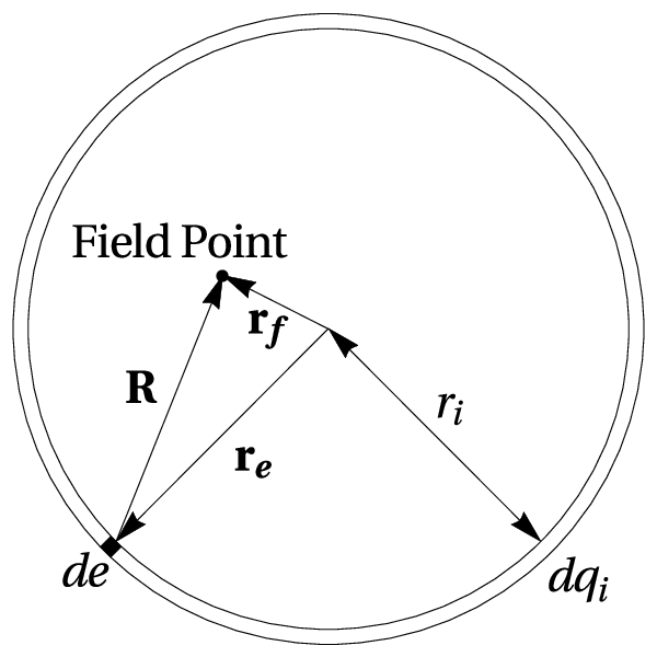
Assume our distribution, when in static equilibrium, is perfectly spherical. In this case, the distribution may be segregated into spherical shells. This is shown in Fig. 1. Each shell contains charge $dq_{i}$ (where $i=1,2,3...N$ labels the shell), and has thickness $dr_{i}$. Taking the limit as $dr_{i}\rightarrow 0$, $N\rightarrow\infty$, all of the $i^{\rm th}$ shell’s charge is uniformly distributed on the shell and concentrated at radius $r_{i}$; then $dq_{i}$ may be thought of as a continuous function of $r_{i}$, $dq_{i}\equiv dq(r_{i})$.

Now assume the shells accelerate (while maintaining their shape in their proper frame). The electric field at a field point, $\mathbf{r}_{f}$, due to a small (point-like) charge $de$ on an accelerating shell of charge that is spherical in its proper frame is[24]

$$\begin{array}[]{l}d\mathbf{E}=\frac{1}{4\pi\epsilon_{0}}\left\{\frac{\hat{R}}{R^{2}}+\left(\frac{1}{2c^{2}R}\left(\frac{\mathbf{r}_{e}\cdot\dot{\mathbf{u}}_{i}}{c^{2}}-1\right)\right)\left((\hat{R}\cdot\dot{\mathbf{u}}_{i})\hat{R}+\dot{\mathbf{u}}_{i}\right)\right.\\ \left.+\frac{3}{8}\frac{\hat{R}}{c^{4}}\left(\left(\hat{R}\cdot\dot{\mathbf{u}}_{i}\right)^{2}-\dot{u}_{i}^{2}\right)+\frac{3(\hat{R}\cdot\dot{\mathbf{u}}_{i})\dot{\mathbf{u}}_{i}}{4c^{2}}+\frac{2\ddot{\mathbf{u}}_{i}}{3c^{2}}+O(R)\right\}de,\end{array}$$

(1)

where $\mathbf{r}_{e}$ is the position of the differential point of charge $de$, $\mathbf{R}=\mathbf{r}_{f}-\mathbf{r}_{e}$, $\hat{R}$ is the unit vector associated with $\mathbf{R}$, and $\mathbf{u}_{i}$ is the velocity the center of the shell, $dq_{i}$, as a function of time. See Fig. 2. In this and all following equations, dots above variables signify time derivatives, bold variables are vectors, hatted variables are unit vectors, and unbolded italic variables are scalars. When an unbolded italic (hatted) variable has the same name as a bold variable, it is the magnitude (unit vector) of that vector.

Integrating $d\mathbf{E}$ over shell $dq_{i}$ yields the electric field due to a rigid spherical shell in arbitrary motion to zeroth order in $R$:

$$\begin{array}[]{c}d\mathbf{E}_{r_{i}\geq r_{f}}=\frac{dq_{i}}{4\pi\epsilon_{0}}\left(\frac{2\ddot{\mathbf{u}}_{i}}{3c^{3}}-\frac{2\dot{\mathbf{u}}_{i}}{3c^{2}r_{i}}+\frac{4\left((\dot{\mathbf{u}}_{i}\cdot\mathbf{r}_{f})\dot{\mathbf{u}}_{i}-\frac{1}{3}\dot{u}_{i}^{2}\mathbf{r}_{f}\right)}{5c^{4}r_{i}}\right)\\ d\mathbf{E}_{r_{i}<r_{f}}=\frac{dq_{i}}{4\pi\epsilon_{0}}\left(\begin{array}[]{c}\frac{\hat{r}_{f}}{r_{f}^{2}}+\frac{2\ddot{\mathbf{u}}_{i}}{3c^{3}}-(\frac{r_{i}^{2}}{6c^{2}r_{f}^{3}}+\frac{1}{2c^{2}r_{f}}\right){\dot{\mathbf{u}}_{i}}+\left(\frac{r_{i}^{4}}{20c^{4}r_{f}^{4}}+\frac{3}{4c^{4}}\right)(\dot{\mathbf{u}}_{i}\cdot\hat{r}_{f})\dot{\mathbf{u}}_{i}+\dot{u}_{i}^{2}\left(\frac{r_{i}^{4}}{40c^{4}r_{f}^{4}}+\frac{r_{i}^{2}}{12c^{4}r_{f}^{2}}-\frac{3}{8c^{4}}\right)\hat{r}_{f}\\ +\left(\frac{r_{i}^{2}}{2c^{2}r_{f}^{3}}-\frac{1}{2c^{2}r_{f}}\right)(\dot{\mathbf{u}}_{i}\cdot\hat{r}_{f})\hat{r}_{f}+\left(-\frac{r_{i}^{4}}{8c^{4}r_{f}^{4}}-\frac{r_{i}^{2}}{4c^{4}r_{f}^{2}}+\frac{3}{8c^{4}}\right)\left(\dot{\mathbf{u}}_{i}\cdot\hat{r}_{f}\right)^{2}\hat{r}_{f}\end{array}\right).\end{array}$$

(2)

Using this result, we can calculate the force from one spherical shell, $dq_{i}$, on another with radius $r_{j}$, $dq_{j}\equiv dq(r_{j})$. Under the assumption of non-relativistic velocity, the force on a differential point of charge $de$ on shell $dq_{j}$ is just $d\mathbf{F}=\int d\mathbf{E}de$. Using the electric field from Eq. 2, most terms integrate to zero and the force from $dq_{i}$ on $dq_{j}$ is

$$d\mathbf{F}_{ij}=\frac{dq_{i}dq_{j}mr_{0}}{q^{2}}\left(\frac{1}{c}\ddot{\mathbf{u}}_{i}-\frac{1}{r_{>}}\dot{\mathbf{u}}_{i}\right)+O(R)$$

(3)

$$r_{0}\equiv\frac{q^{2}}{6\pi\epsilon_{0}mc^{2}},$$

(4)

where $r_{>}$ is the greater of the radii of the spheres ($r_{i}$ and $r_{j}$), and $r_{0}$ is a constant with units of length, which will simplify results that follow. $m$ is the inertial mass of the total distribution (what one would measure in a laboratory by taking the ratio of the external force to the center-of-mass acceleration); $q\equiv\int dq_{i}$ is the integrated charge of the distribution. For an electron, $r_{0}\approx 1.88$ fm.

Integrating over all of the source shells ($dq_{i}$), the net force on shell $dq_{j}$, including its self-force ($r_{i}=r_{j}$), is

$$d\mathbf{F}_{j}=d\mathbf{F}_{e}+d\mathbf{F}_{b}+\frac{mr_{0}dq_{j}}{q^{2}}\left(\int\frac{\ddot{\mathbf{u}}_{i}}{c}dq_{i}-\int\frac{\dot{\mathbf{u}}_{i}}{r_{>}}dq_{i}\right).$$

(5)

Here and below, unless otherwise stated, integrals cover the whole distribution. I’ve included an arbitrary external force $d\mathbf{F}_{e}$ and the necessary binding force $d\mathbf{F}_{b}$ to keep $dq_{j}$ concentric (and from exploding). Now say $dq_{j}$ is allowed to displace from its equilibrium position. If the charge is stable against such displacements, the binding force must change to return the sphere to concentricity. Leaving $d\mathbf{F}_{b}$ as the equilibrium binding force, define a “restoring force,” $d\mathbf{F}_{r}$, as the change in the net force on $dq_{j}$ due to the displacement from equilibrium. Note that a deviation from concentricity will also change the self-electromagnetic force on $dq_{j}$, which is also included in $d\mathbf{F}_{r}$. Therefore, with the addition of $d\mathbf{F}_{r}$, Eq. 5 is fairly general, even allowing small displacements of the constituent spherical shells from concentricity.

At this point, it is convenient to define a parameter that quantifies the net displacement of the spherical shells from equilibrium, which will be related to the total dipole moment of the charge. Call $\mathbf{r}_{ci}$ the position of the center of spherical shell, $dq_{i}$, and define

$$\mathbf{r}_{a}\equiv\frac{1}{q}\int\left(\mathbf{r}_{ci}-\mathbf{r}\right)dq_{i}=\frac{1}{q}\int\mathbf{r}_{ci}dq_{i}-\mathbf{r},$$

(6)

where $q$ is the total charge of the distribution and $\mathbf{r}$ is the position of the center of mass of the distribution. The net dipole moment of the distribution about the origin may be written as $\mathbf{p}=q(\mathbf{r}+\mathbf{r}_{a})$, and about the center of mass, $\mathbf{p}_{cm}=q\mathbf{r}_{a}$. Noting that the velocity of the center of the $i^{\rm th}$ shell is $\mathbf{u}_{i}=\dot{\mathbf{r}}_{ci}$, and taking successive time derivatives, Eq. 6 yields

$$\begin{array}[]{c}\mathbf{u}_{a}\equiv\frac{1}{q}\int\mathbf{u}_{i}dq_{i}-\mathbf{u}\\ \dot{\mathbf{u}}_{a}\equiv\frac{1}{q}\int\dot{\mathbf{u}}_{i}dq_{i}-\dot{\mathbf{u}}\\ \ddot{\mathbf{u}}_{a}\equiv\frac{1}{q}\int\ddot{\mathbf{u}}_{i}dq_{i}-\ddot{\mathbf{u}}.\end{array}$$

(7)

At this point, no assumption has been made that the charge on each shell is constant, but Eqs. 7 imply that any radial transfer of charge between shells does not change the total dipole moment. It should be noted that any time variation of the charge on each shell must also be slow compared the size of the charge divided by $c$, so that Eq. 3 remains valid using the charge at the present time.

Evaluating the first integral in Eq. 5

$$\begin{array}[]{lll}d\mathbf{F}_{j}&=&d\mathbf{F}_{e}+d\mathbf{F}_{b}+d\mathbf{F}_{r}\\ &+&\frac{mr_{0}dq_{j}}{q^{2}}\left(\frac{q}{c}(\ddot{\mathbf{u}}+\ddot{\mathbf{u}}_{a})-\int\frac{\dot{\mathbf{u}}_{i}}{r_{>}}dq_{i}\right).\end{array}$$

(8)

Integrating both sides over all spherical shells, $dq_{j}$, yields the net force on the charge distribution:

$$\mathbf{F}=\mathbf{F}_{e}+\mathbf{F}_{b}+mr_{0}\left(\frac{1}{c}(\ddot{\mathbf{u}}+\ddot{\mathbf{u}}_{a})-\frac{1}{q^{2}}\iint\frac{\dot{\mathbf{u}}_{i}}{r_{>}}dq_{i}dq_{j}\right).$$

(9)

where $\mathbf{F}_{b}=\int d\mathbf{F}_{b}+\int d\mathbf{F}_{r}$.

If the distribution is stable, the shells will oscillate around concentricity. As different spherical shells may oscillate with different phases, I transform to the frequency domain in order to more easily account for these phase differences. The following convention for the Fourier transform and transform of a product of functions is used:

$$\begin{array}[]{c}f(\omega)=\mathcal{F}(f(t))=\frac{1}{\sqrt{2\pi}}\int_{-\infty}^{\infty}f(t)e^{-i\omega t}dt\\ \mathcal{F}(f(t)g(t))=\frac{1}{\sqrt{2\pi}}f(\omega)*g(\omega),\end{array}$$

(10)

where * denotes a convolution in $\omega$ space (a product of more than two functions produces factors of $1/\sqrt{2\pi}$ for each product). In the frequency domain, Eq. 9 is then

$$\begin{array}[]{lll}\mathbf{F}(\omega)&=&\mathbf{F}_{e}+\mathbf{F}_{b}+\frac{mr_{0}}{c}(\ddot{\mathbf{u}}+\ddot{\mathbf{u}}_{a})\\ &-&\frac{mr_{0}}{2\pi q^{2}}\iint\frac{\dot{\mathbf{u}}_{i}}{r_{>}}*(dq_{i}*dq_{j}),\end{array}$$

(11)

where $\omega$ dependence on the right hand side is implied. Now assume the motion of the centers of the spheres can be described as

$$\mathbf{r}_{ci}(r_{i},\omega)=\mathbf{r}(\omega)+f_{q}(r_{i},\omega)\mathbf{r}_{a}(\omega),$$

(12)

where, again, $r_{i}$ is the radius of shell $dq_{i}$, and $f_{q}$ is a scalar complex function that describes the relative amplitude and phase of the displacement of the shell with respect to the net dipolar motion. This is a statement that the displacement of an individual spherical shell, $\mathbf{r}_{ci}-\mathbf{r}$, lies along the net vector $\mathbf{r}_{a}$, is proportional to $\mathbf{r}_{a}$, and the relative phase/magnitude of the displacement of each shell to the net dipolar displacement only depends on $\omega$. This “linearity” is similar to linear models of dielectric materials, where the relative permittivity is a function of $\omega$. Note we implicitly ignore non-dipolar motion, i.e. flexing of the spheres and motion not in the direction of $\mathbf{r}_{a}$, which would result in higher order moments.

As an aside, $f_{q}$ is constrained by the definition of $\mathbf{r}_{a}$ in Eq. 6, and with some algebra, one finds

$$\frac{1}{q}\int f_{q}(r_{i})dq_{i}=1.$$

(13)

The function $f_{q}$ can be viewed as describing the relative stiffness of parts of the distribution, and is set as a parameter of the model; Eq. 13 sets the overall scale of $f_{q}$.

Using Eq. 12, Eq. 11 becomes

$$\begin{array}[]{lll}\mathbf{F}(\omega)&=&\mathbf{F}_{e}+\mathbf{F}_{b}+\frac{mr_{0}}{c}(\ddot{\mathbf{u}}+\ddot{\mathbf{u}}_{a})\\ &-&\left(mk_{0}*\dot{\mathbf{u}}+\frac{mr_{0}}{2\pi q^{2}}\iint\frac{f_{q}(r_{i})\dot{\mathbf{u}}_{a}}{r_{>}}*(dq_{i}*dq_{j})\right)\end{array}$$

(14)

$$k_{0}\equiv\frac{r_{0}}{2\pi q^{2}}\iint\frac{dq_{i}*dq_{j}}{r_{>}}.$$

(15)

If the $dq$’s are constant in time, the convolutions can be performed noting they transform as $dq_{\rm const}(t)\rightarrow\sqrt{2\pi}dq_{\rm const}\delta(\omega)$. Therefore, in the case of constant $dq$, one obtains the net force on the distribution

$$\mathbf{F}(\omega)=\mathbf{F}_{e}+\mathbf{F}_{b}+\frac{mr_{0}}{c}(\ddot{\mathbf{u}}+\ddot{\mathbf{u}}_{a})-m\left(k_{0}\dot{\mathbf{u}}+k_{1}\dot{\mathbf{u}}_{a}\right),$$

(16)

where

$$k_{1}\equiv\frac{r_{0}}{q^{2}}\iint\frac{f_{q}(r_{i})}{r_{>}}dq_{j}dq_{i}.$$

(17)

Identifying the force on the left hand side as the momentum imparted to the charge, the force must also be

$$\begin{array}[]{rcl}\mathbf{F}(\omega)&=&\int\dot{{\mathbf{u}}}_{j}dm_{qj}=m_{q}\dot{\mathbf{u}}+\dot{\mathbf{u}}_{a}\int f_{q}(r_{j})dm_{qj}\\ &=&m_{q}\dot{\mathbf{u}}+mk_{\rm ma}\dot{\mathbf{u}}_{a},\end{array}$$

(18)

where $dm_{qj}$ is the inertial mass inherent to the charge $dq_{j}$, $m_{q}\equiv\int dm_{qj}$, and $k_{\rm ma}\equiv\frac{1}{m}\int f_{q}(r_{j})dm_{qj}$. Note that $m_{q}$ is not what is measured as the inertial mass of the distribution in the laboratory, since the inertial mass due to the charge’s field is not included in $m_{q}$. This is discussed more below.

The binding force may be viewed as the momentum imparted to the charge by other matter attached to the charge distribution; this matter is responsible for binding the charge (canceling the self-electromagnetic forces) at equilibrium. For simplicity, I assume the other matter travels at the center-of-mass velocity throughout the distribution. Otherwise, we would need to track the dipolar motion of the other mass as well, which is beyond the scope of this paper.

Without knowing more of its nature, we can write the differential binding force on $dq_{j}$ as $d\mathbf{F}_{b}=-dm_{{\rm other},j}\dot{\mathbf{u}}$, where $dm_{{\rm other},j}\dot{\mathbf{u}}$ is the force by $dq_{j}$ on the “other” matter as the other matter accelerates; then apply Newton’s third law. Note that $dm_{{\rm other},j}$ is not necessarily located on the shell $dq_{j}$; consider it the portion of the other mass over the entire distribution responsible for keeping $dq_{j}$ at its equilibrium position. Integrating, $\mathbf{F}_{b}=\int d\mathbf{F}_{b}=-m_{\rm other}\dot{\mathbf{u}}$. The function, $dm_{{\rm other},j}=dm_{\rm other}(r_{j})$, must be set as a parameter of the model.

Implementing these relations, and rearranging Eq. 16

$$\begin{array}[]{lll}(m_{q}+mk_{0}+m_{\rm other})\dot{\mathbf{u}}&=&\mathbf{F}_{e}+\frac{mr_{0}}{c}(\ddot{\mathbf{u}}+\ddot{\mathbf{u}}_{a})\\ &-&m\left(k_{\rm ma}+k_{1}\right)\dot{\mathbf{u}}_{a}.\end{array}$$

(19)

In the laboratory, the total inertial mass is measured (in the low velocity limit) by taking the ratio of $\mathbf{F}_{e}$ to $\dot{\mathbf{u}}$. Experimentally, of course, one would need to first remove the effects of the field reaction terms proportional to $\ddot{\mathbf{u}}$, and terms proportional to $\dot{\mathbf{u}}_{a}$ and $\ddot{\mathbf{u}}_{a}$. One may use this fact in Eq. 19 to equate the coefficient in front of $\dot{\mathbf{u}}$ to the observed inertial mass $m$,

$$m=m_{q}+mk_{0}+m_{\rm other}.$$

(20)

Eq. 19 then simplifies to

$$\dot{\mathbf{u}}=\frac{1}{m}\mathbf{F}_{e}+\frac{r_{0}}{c}(\ddot{\mathbf{u}}+\ddot{\mathbf{u}}_{a})-\left(k_{\rm ma}+k_{1}\right)\dot{\mathbf{u}}_{a}.$$

(21)

This is the low-velocity equation of motion for the center of mass of a small spherical distribution of charge, if the charge per shell is constant in time.

Another aside: Eq. 20 acts as a constraint on the mass terms. Therefore, if $m_{\rm other}$ is set, then $m_{q}$ is automatically set by Eq. 20, or vice versa; any mass model that is chosen for $dm_{q}$ and $dm_{\rm other}$ must satisfy Eq. 20 for consistency.

The constant, $k_{0}m$, can be identified as the inertial mass of the self-electromagnetic field, as it is the coefficient of the acceleration that comes from the momentum transfer between the self-electromagnetic field and the charge. Relabeling Eq. 20 for clarity, $m=m_{q}+m_{\rm field}+m_{\rm other}$.

In order to fully determine the motion of the distribution, we need a second dynamic equation for $\mathbf{r}_{a}$. In order to do this, we need to make some assumption on the mass model used for the charge, i.e. $dm_{qj}$. Again, I note that $dm_{qj}$ is the inertial mass of $dq_{j}$ without its field. We assume one of two cases, (1) $dm_{qj}$ is a function of $dq_{j}$, and is non-zero for a shell of non-zero $dq_{j}$; (2) $dm_{qj}=0$. First, we treat case 1, and case 2 is discussed below. Under case 1, and imposing Newton’s second law on $dq_{j}$, Eq. 8 is also equal to

$$d\mathbf{F}_{j}=\dot{\mathbf{u}}_{j}dm_{qj}.$$

(22)

Replacing $d\mathbf{F}_{j}$ in Eq. 8, subtracting both sides by $\dot{\mathbf{u}}dm_{qj}$, and multiplying by the factor $dq_{j}/dm_{qj}$ (assuming a well defined limit in the case of $dq_{j}\rightarrow 0$):

$$\begin{array}[]{lll}(\dot{\mathbf{u}}_{j}-\dot{\mathbf{u}})dq_{j}&=&-\dot{\mathbf{u}}dq_{j}+\frac{dq_{j}}{dm_{qj}}[d\mathbf{F}_{e}+d\mathbf{F}_{b}+d\mathbf{F}_{r}\\ &+&\frac{mr_{0}dq_{j}}{q^{2}}\left(\frac{q}{c}(\ddot{\mathbf{u}}+\ddot{\mathbf{u}}_{a})-\int\frac{\dot{\mathbf{u}}_{i}}{r_{>}}dq_{i}\right)].\end{array}$$

(23)

Define $\rho_{qm}(r_{j})\equiv\frac{dq_{j}}{dm_{qj}}$ as the charge density divided by its inertial mass density as a function of the radius of sphere $j$. Integrating over $dq_{j}$ gives:

$$\begin{array}[]{lll}q\dot{\mathbf{u}}_{a}&=&-q\dot{\mathbf{u}}+\int\rho_{qm}(r_{j})[d\mathbf{F}_{e}+d\mathbf{F}_{b}+d\mathbf{F}_{r}\\ &+&\frac{mr_{0}dq_{j}}{q^{2}}\left(\frac{q}{c}(\ddot{\mathbf{u}}+\ddot{\mathbf{u}}_{a})-\int\frac{\dot{\mathbf{u}}_{i}}{r_{>}}dq_{i}\right)].\end{array}$$

(24)

Transforming to the frequency domain, we have

$$\begin{array}[]{lll}q\dot{\mathbf{u}}_{a}(\omega)&=&-q\dot{\mathbf{u}}+\int\frac{\rho_{qm}(r_{j})}{\sqrt{2\pi}}*[d\mathbf{F}_{e}+d\mathbf{F}_{b}+d\mathbf{F}_{r}\\ &+&\frac{mr_{0}dq_{j}}{\sqrt{2\pi}q^{2}}*\left(\frac{q}{c}(\ddot{\mathbf{u}}+\ddot{\mathbf{u}}_{a})-\int\frac{\dot{\mathbf{u}}_{i}*dq_{i}}{\sqrt{2\pi}r_{>}}\right)].\end{array}$$

(25)

Assuming the $dq$’s are constant in time, using the fact that $d\mathbf{F}_{b}=-dm_{\rm other}\dot{\mathbf{u}}$, and using Eq. 12, we obtain

$$\begin{array}[]{lll}q\dot{\mathbf{u}}_{a}(\omega)&=&-q\dot{\mathbf{u}}+\int\rho_{qm}(r_{j})(d\mathbf{F}_{e}+d\mathbf{F}_{r})-qk_{b0}\dot{\mathbf{u}}\\ &+&k_{e0}\frac{qr_{0}}{c}(\ddot{\mathbf{u}}+\ddot{\mathbf{u}}_{a})-q(k_{a0}\dot{\mathbf{u}}+k_{a1}\dot{\mathbf{u}}_{a})\end{array}$$

(26)

	$\displaystyle k_{b0}\equiv\frac{1}{q}\int\rho_{qm}(r_{j})dm_{{\rm other},j}$		(27)
	$\displaystyle k_{e0}\equiv\frac{m}{q^{2}}\int\rho_{qm}(r_{j})dq_{j}$		(28)
	$\displaystyle k_{a0}\equiv\frac{mr_{0}}{q^{3}}\iint\frac{\rho_{qm}(r_{j})}{r_{>}}dq_{i}dq_{j}$		(29)
	$\displaystyle k_{a1}\equiv\frac{mr_{0}}{q^{3}}\iint\frac{\rho_{qm}(r_{j})f_{q}(r_{i})}{r_{>}}dq_{i}dq_{j}.$		(30)

Divide by $q$ and gather the $\dot{\mathbf{u}}_{a}$ terms,

$$\begin{array}[]{c}(1+k_{a1})\dot{\mathbf{u}}_{a}(\omega)=\frac{1}{q}\int\rho_{qm}(r_{j})(d\mathbf{F}_{e}+d\mathbf{F}_{r})\\ -(1+k_{a0}+k_{b0})\dot{\mathbf{u}}+k_{e0}\frac{r_{0}}{c}(\ddot{\mathbf{u}}+\ddot{\mathbf{u}}_{a}).\end{array}$$

(31)

Now assume the displacement of each spherical shell is small, so the restoring force can be assumed linear in the displacement of the center of shell $j$ from the center of mass ($\mathbf{r}_{cj}-\mathbf{r}$):

$$d\mathbf{F}_{r}(r_{j})=-k_{rr}(r_{j})\frac{mc^{2}}{r_{0}^{3}}(\mathbf{r}_{cj}-\mathbf{r})dr_{j},$$

(32)

where $k_{rr}$ is a positive function of the radius; $k_{rr}$ describes the strength of the restoring force and is set as a model parameter. Eq. 32 is the first term in the power series expansion about equilibrium for an arbitrary smooth force that depends only on the position of the center of the shell. Evaluating the restoring integral,

$$\frac{1}{q}\int\rho_{qm}(r_{j})d\mathbf{F}_{r}=-k_{r}\frac{c^{2}}{r_{0}^{2}}\mathbf{r}_{a}$$

(33)

$$k_{r}\equiv\frac{m}{qr_{0}}\int\rho_{qm}(r_{j})k_{rr}(r_{j})f_{q}(r_{j})dr_{j}.$$

(34)

To determine the dynamics of $\mathbf{r}_{a}$ in an external electric field, $\mathbf{E}$, set $d\mathbf{F}_{e}=dq_{j}\mathbf{E}$. This assumes that $\mathbf{E}$ is constant over the displacements $\mathbf{r}_{cj}-\mathbf{r}$, and the source of $\mathbf{E}$ is outside the entire distribution. With these assumptions, the external force integral becomes

$$\frac{1}{q}\int\rho_{qm}(r_{j})d\mathbf{F}_{e}=k_{e1}\frac{q}{m}\mathbf{E},$$

(35)

where $k_{e1}=k_{e0}$. If the source of the electric field is within the outermost sphere, the treatment is still valid, but the integral truncates at the position where the source of the electric field is located, and $k_{e1}$ is no longer equal to $k_{e0}$. Inserting the external and restoring force, and rearranging Eq. 31, we have

$$\dot{\mathbf{u}}_{a}(\omega)=k_{m1}\frac{q}{m}\mathbf{E}-k_{ar}\frac{c^{2}}{r_{0}^{2}}\mathbf{r}_{a}-k_{au}\dot{\mathbf{u}}+k_{m0}\frac{r_{0}}{c}(\ddot{\mathbf{u}}+\ddot{\mathbf{u}}_{a})$$

(36)

$$k_{m0}\equiv k_{e0}/\left(1+k_{a1}\right)$$

(37)

$$k_{m1}\equiv k_{e1}/\left(1+k_{a1}\right)$$

(38)

$$k_{ar}\equiv k_{r}/\left(1+k_{a1}\right)$$

(39)

$$k_{au}\equiv\left(1+k_{a0}+k_{b0}\right)/\left(1+k_{a1}\right).$$

(40)

Eqs. 21 and 36 are the low-velocity center-of-mass and dipolar equations motion of a small (zeroth order in $R$) spherically distributed charge in an electric field where the displacement of its spherical constituents from concentricity is small enough to assume a linear restoring force, and the response of the spherical constituents is linear with respect to the bulk dipolar motion.

Assuming $f_{q}$ is real (individual motions are completely in or out of phase with net dipolar motion about the center of mass), and its magnitude does not vary with frequency, then the same treatment may be performed in the time domain, and the equations maintain the same form as they do in the frequency domain, without the need of constraining the $dq$’s to be constant.

Depending on the choice of charge distribution ($dq_{j}=dq(r_{j})$) and the choice of $dm_{{\rm other}}(r_{j})$, Eq. 20 may require the charge mass model to have $dm_{qj}>0$, $dm_{qj}<0$, or $dm_{qj}=0$ (i.e. the charge’s mass is entirely due to its self-electromagnetic field). In the case of $dm_{q}=0$, $\rho_{qm}$ is ill defined. This special case may be treated in the following way: Eq. 22 becomes $dF_{j}=0$, and this may be inserted into Eq. 8. The result is somewhat simpler: in the case of $dm_{qj}=0$, Eq. 36 remains the same, but the constants are simplified,

$${\rm In~the~case:~}dm_{qj}=0$$

(41)

$$k_{m0}=1/k_{1}$$

(42)

$$k_{m1}=1/k_{1}$$

(43)

$$k_{ar}=k_{r0}/k_{1}$$

(44)

$$k_{au}=\left(k_{0}+\frac{m_{\rm other}}{m}\right)/k_{1}$$

(45)

$$k_{r0}\equiv\frac{1}{r_{0}}\int k_{rr}(r_{j})f_{q}(r_{j})dr_{j}.$$

(46)

References

- [1] H. Lorentz, Arch. Neerl. Sci. Exactes Nat. 25, 363 (1892).
- [2] J. Larmor, Philos. Mag. 44, 503 (1897).
- [3] O. Heaviside, Nature 67, 6 (1902).
- [4] M. Abraham, Ann. Phys. 14, 236 (1904).
- [5] M. Abraham, Theorie der Elektrizitat, Vol. II (Teubner, Leipzig, 1905).
- [6] M. V. Laue, Ann. Phys. 28, 436 (1909).
- [7] G. Schott, Electromagnetic Radiation (Cambridge University Press, Cambridge, 1912).
- [8] H. Poincare, Rendiconti del Circolo Matematico di Pulermo 21, 129 (1906).
- [9] P. Dirac, Proc. R. Soc. London Ser. A 167, 148 (1938).
- [10] J. D. Jackson, Classical Electrodynamics 3rd Ed. (John Wiley and Sons, Inc, New York, 1998).
- [11] R. Medina, J. Phys. A 39, 3801 (2006), URL http://stacks.iop.org/0305-4470/39/i=14/a=021.
- [12] F. Rohrlich, Phys. Rev. E 77, 046609 (2008), URL http://link.aps.org/doi/10.1103/PhysRevE.77.046609.
- [13] J. M. Aguirregabiria, J. Llosa, and A. Molina, Phys. Rev. D 73, 125015 (2006), ISSN 1550-7998.
- [14] H. Essen and J. C. E. Sten, Eur. J. Phys. 36, 055029 (2015), ISSN 0143-0807.
- [15] M. R. Ferris and J. Gratus, J. Math. Phys. 52, 092902 (2011), ISSN 0022-2488.
- [16] J. A. Heras, Phys. Lett. A 314, 272 (2003), ISSN 0375-9601.
- [17] F. Rohrlich, Am. J. Phys. 68, 1109 (2000), ISSN 0002-9505.
- [18] F. Rohrlich, Phys. Rev. D 63, 127701 (2001), ISSN 0556-2821.
- [19] A. M. Steane, Am. J. Phys. 83, 256 (2015a), ISSN 0002-9505.
- [20] A. M. Steane, Phys. Rev. D 91, 065008 (2015b), ISSN 1550-7998.
- [21] A. M. Steane, Am. J. Phys. 83, 703 (2015c), ISSN 0002-9505.
- [22] D. Villarroel, Phys. Rev. E 66, 046624 (2002), ISSN 1539-3755.
- [23] F. Rohrlich, Am. J. Phys. 65, 1051 (1997).
- [24] A. D. Yaghjian, Relativistic Dynamics of a Charged Sphere: Updating the Lorentz-Abraham Model (Springer-Verlag, Berlin, 1992).
- [25] C. R. Galley, A. K. Leibovich, and I. Z. Rothstein, Phys. Rev. Lett. 105, 094802 (2010), ISSN 0031-9007.
- [26] P. Forgács, T. Herpay, and P. Kovács, Phys. Rev. Lett. 109, 029501 (2012), URL http://link.aps.org/doi/10.1103/PhysRevLett.109.029501.
- [27] C. R. Galley, A. K. Leibovich, and I. Z. Rothstein, Phys. Rev. Lett. 109, 029502 (2012), URL http://link.aps.org/doi/10.1103/PhysRevLett.109.029502.