High-Energy Evolution To Three Loops
Abstract
The Balitsky-Kovchegov equation describes the high-energy growth of gauge theory scattering amplitudes as well as nonlinear saturation effects which stop it. We obtain the three-loop corrections to the equation in planar super Yang-Mills theory. Our method exploits a recently established equivalence with the physics of soft wide-angle radiation, so-called non-global logarithms, and thus yields at the same time the three-loop evolution equation for non-global logarithms. As a by-product of our analysis, we develop a Lorentz-covariant method to subtract infrared and collinear divergences in cross-section calculations in the planar limit. We compare our result in the linear regime with a recent prediction for the so-called Pomeron trajectory, and compare its collinear limit with predictions from the spectrum of twist-two operators.
1 Introduction
In high-energy scattering, the aspect of a particle depends on the energy scale at which it is probed. In hadronic collisions this effect can be seen in the well known energy dependence of parton distribution functions. The energy dependence can be accessed in a more detailed way by looking at less inclusive observables, for example ones probing correlations between very different rapidities, opening a window on the transverse structure of the projectile. One then encounters another fundamental evolution equation of QCD, the Balitsky-Fadin-Kuraev-Lipatov (BFKL) equation [1, 2].
In contrast to other evolution equations, which are typically linear, nonlinear effects can also play a role in rapidity evolution: once scattering at a given impact parameter has reached opacity, it must saturate. A nonlinear evolution equation which incorporates such effects within perturbation theory has been derived by Balitsky and Kovchegov [3, 4]. Asymptotically, saturation may occur at distances shorter than the nonperturbative scale , justifying the use of perturbation theory [5, 6]. For many observables, such as inclusive jet correlations or deep inelastic scattering, perturbation theory is also justified by the large momentum transfer in the problem (see for example [7, 8] and references therein). The need to control higher order corrections, and the need to better understand the theory at finite coupling, motivate a deeper look into the perturbative series.
The next-to-leading-order evolution equation has been known for some time [9]. It reproduces, in the appropriate limit, the next-to-leading order BFKL Pomeron trajectory [10, 11]. A notable feature is that the degree of nonlinearity and its complexity increases with each new order in perturbation theory. This is a rather unfamiliar situation which makes it unclear how to best formulate the equation at finite coupling. Furthermore, the corrections have turned out to be numerically large. This has been attributed to collinear effects, suggesting a possibility to resum them at higher orders at both the linear (BFKL) and nonlinear level [12, 13, 14]. In order to shed light on these issue, and to critically assess the quality of proposed resummations, higher-loop data is clearly highly desirable.
The aim of this paper is to initiate a systematic study of the Balitsky-Kovchegov and BFKL equations at three loops and beyond. Specifically, as a first step, we will derive its three-loop (next-to-next-to-leading order) correction in the planar limit of super Yang-Mills (SYM). This calculation is made possible by recent conceptual and technological developments in the calculation of scattering amplitudes. Our methods remain however essentially diagrammatic and we expect them to prove applicable to QCD in a next step.
The SYM model is an ideal stepping stone for several reasons. First, partial cross-checks are available due to a recent and highly remarkable prediction of the Pomeron trajectory exploiting integrability in this model [15, 16]. Such tests are valuable both from the perturbative and integrability perspective. At the nonlinear level, the interactions to be predicted are related to structure constants [17], soon to be within reach of similar methods. Together with the AdS/CFT correspondence at strong coupling [18], these hint at a possible exact description of the Pomeron and its interactions at finite coupling in this model.
1.1 High-energy scattering, soft gluons, and non-global logarithms
A modern description of high-energy forward scattering is based on the eikonal approximation: fast projectiles and targets are approximated by null Wilson lines . More precisely, by a collection of such Wilson lines, reflecting the transverse structure of the colliding objects at the given rapidity scale [3]. It is simple to translate this language to that of classic Regge theory: the reggeized gluon is the state sourced by (the logarithm of) a null Wilson line [19].
The three-loop calculation in this paper is enabled by a recently established correspondence with the physics of wide-angle soft radiation, sometimes called “non-global logarithms.” Consider the QCD decay of a color singlet state like a virtual photon or boson, with energy . A representative observable, sensitive to soft wide-angle radiation, is the probability to not find radiation with energy above a cutoff within an exclusion region (see fig. 1). If the cutoff is low, this probability is small and controlled in the planar approximation (’t Hooft limit ) by the Banfi-Marchesini-Smye evolution equation [20]:
| (1) |
This resums large logarithms . Here , and the subscripts denote the angles of outgoing partons; the dipole is a function of two angles which can be interpreted (see below) as the trace of a color dipole at angles and .
The basic physics of this equation is that the color flow, and therefore the energy flow, is affected by radiation of an extra gluon at angle . The observable, through the exclusion region , is encoded by the infrared boundary condition that when either or are in . Qualitatively, the evolution leads to an increased effective size of the exclusion region, as radiation near the allowed boundaries become more and more in danger of leaking out.11 1 The form (1) is valid provided that is smooth enough that no jets are forced to be narrow. This is assumed here in order to avoid further subtractions of collinear singularities as in the original setup [20], thereby focusing on soft wide-angle radiation and preserving the most symmetrical form of the equation.
This equation is mathematically equivalent to the Balitsky-Kovchegov equation, which governs the rapidity dependence of perturbative high-energy scattering near the forward direction. In this context, the trivial fixed point represents a transparent target, which is unstable: by linearizing in the departure , which gives the BFKL equation, one finds a growing solution known as the BFKL Pomeron. The nonlinear term then accounts for a class of saturation effects which stop the growth (locally in the transverse plane) toward the attractive, opaque, fixed-point .
The nonlinear term in both equations share a similar physical origin: in both cases one is interested in the probability that something does not happen, while many possibly complicated things may happen [21]. Indeed, to describe the probability to not radiate in a certain region, one must keep track of all allowed radiation, which is what the nonlinear term of eq. (1) produces. Similarly, in near-forward scattering, one measures the probability for a projectile to not be destroyed at a given impact parameter. The two evolutions share other physical similarities: both are dominated by soft gluons, and both feature “opaque” and “transparent” regimes.
Given these similarities, it seems natural to expect a relationship between these two problems. The geometry is however different. To establish a rigorous map turns out to require a conformal transformation [22, 23], which equates detector measurements at infinity with the physics of a fast particle crossing a Lorentz-contracted target (also known as a shockwave). This had been used notably by Hofman and Maldacena and others to describe detector measurements in conformal field theories [24, 22, 25] and at the same time gain new insight into high-energy scattering. This conformal transformation is just the stereographic projection of a two-sphere onto the transverse impact parameter plane:
| (2) |
Here is an arbitrary mass scale and is rapidity. Under this dictionary, the Banfi-Marchesini-Smye equation (1) becomes precisely the Balitsky-Kovchegov equation, as was noted early on [26].
In this paper we will exploit this correspondence and work exclusively on the non-global logarithm side, which is technically advantageous due to a body of knowledge on the infrared and collinear factorization of amplitudes and cross-sections. This correspondence was emphasized and tested explicitly at two-loops in [23], where the full two-loop BFKL/BK equation (including running coupling effects and non-planar corrections) was re-derived starting from non-global logarithm problem.
The evolution equation (1) at finite coupling is best viewed as a renormalization group (RG) equation:
| (3) |
where the color density matrix, or weighted cross-section , is defined operationally by weighing each final state parton by a color rotation [23] (see also [27]). These color rotations can be understood as Wilson lines ) accounting for the effect of more infrared radiation (these Wilson lines connect the decaying state in the matrix element and its conjugate) [28, 29]. In the planar limit, the color factors reduce to products of color dipoles and the color density matrix simplifies to a single function of only two angles, as shown in fig. 1, which illustrates the “” term in eq. (1).
In both eqs. (1) and (3), is an infrared cutoff below which all radiation is inclusive. In our practical calculation we will work within dimensional regularization to (). Then the cutoff appears in a renormalization procedure. Following standard procedure, this is equivalent to integrating the RG equation from the deep infrared:
| (4) |
where, writing for the running coupling in dimensions, one can see that the integral produces poles. The subtraction then cancels the poles in the bare amplitude so as to make finite as . That the divergences exponentiate in precisely this way was proved to all orders in ref. [23], exploiting known results on the factorization of soft partons [30, 31]. The upshot of eq. (4) is that we can use the poles in the dimensionally regulated weighted cross-section to read off the non-global-logarithm/Balitsky-Kovchegov kernel . Note that this is identical to the standard procedure to extract (ultraviolet) anomalous dimensions of local operators, by using their poles. The fact that divergences (either infrared or ultraviolet) are controlled by renormalization group equations is of course due to the Wilsonian decoupling between physics at different scales.
This paper is organized as follows. In section 2 we introduce useful notations for soft currents and phase space integrals. In section 3 we revisit the two-loop calculation, improving on previous treatments by introducing a scheme where Lorentz symmetry is manifest at each step; under the correspondence with the Regge limit, this is equivalent to maintaining the conformal symmetry of the BK equation. In section 4 we perform the three-loop calculation, paying special attention to the combinatorics of subdivergences and their cancellations, culminating in the final result for the nonlinear equation in subsection 4.6. In section 5 we analyze its linearized limit, compute its eigenvalues, and compare it with integrability predictions. Finally section 6 contains our concluding remarks. In three appendices, we record the one-loop double soft current squared (appendix A), we detail our algorithm to compute finite angular or transverse integrals (appendix B), and record the three-loop eigenvalue (appendix C).
2 Notations
The calculation of requires squared matrix elements for emitting soft partons off two color-correlated parents (“dipole”), the so-called soft currents. The evolution equation, just like the soft currents, is universal and does not depend on details of the underlying short-distance process, only on the color charges and angles of the outgoing partons. Final states are then weighted, in the planar limit, by a product of color dipoles (see fig. 1). For each such product, it is useful to pull out a universal factor which accounts for its dimensionality and most singular limits. We thus write the contribution from the soft current with soft partons to the -loop cross-section, starting from a parent dipole along directions and , as:
| (5a) | |||||
| (5b) | |||||
| (5c) | |||||
Here loops are counted in powers of , , and phase-space integrals are normalized as . For the Mandelstam invariants and their multi-index generalizations, we let:
| (6) |
All invariants will always be positive (timelike), since we assume a color singlet initial state. Naturally for our setup, on-shell momenta will be split into an energy and angular parts : where is null. The Lorentz-invariant phase space measure correspondingly splits into an energy and angular parts:
| (7) |
For angles we write , which runs between 0 and 1. Throughout, we will use the subscripts , , to index radiated gluons.
The various factors of in our definitions have been chosen to simplify limits and preclude unnecessary ’s in integrated expressions. For example, for one soft gluon, is the square of the well-known eikonal soft current. Including the factor from the color sum, this evaluates to
| (8) |
For two soft partons one needs the square of the double soft current, described for example in [30]. The result after squaring it and including the fermions and scalars of SYM can be borrowed from formulas of ref. [23] (section 3), also rederived below in subsection 4.1:
| (9) |
One can easily verify that this factorizes in soft limits:
| (10) |
Our three-loop computation builds on the one-loop corrections to and the tree-level three-parton amplitude , which will be efficiently obtained as described below.
3 Two-loop evolution: fixing a convenient scheme
The next-to-leading order correction to the Balitsky-Kovchegov equation was obtained in QCD and SYM in [9, 32]. It was postulated [33] and verified explicitly that the same kernel governs non-global logarithms [23].
In the latter reference, soft partons were organized in terms of their energies. Because “energy” is not Lorentz invariant, this scheme did not manifest Lorentz invariance, which had to be restored manually through a finite renormalization (guaranteed to exist given the Lorentz invariance of the underlying theory). This is formally similar to the transformation used to reach to the so-called conformal scheme in the BK literature [32]. Indeed the mapping (2) interchanges the Lorentz and conformal symmetry of the two problems.
Here we improve on this by using explicitly Lorentz-invariant cutoffs. To fully define the scheme in which our three-loop result will apply, we thus quickly revisit the two-loop calculation.
3.1 One-loop in Lorentz-invariant form
The idea is to define the evolution so that its exponentiation generates the emission probability of a soft gluon, in the soft approximation, integrated over a complete phase space region bounded by a Lorentz-invariant cutoff. For example, at one-loop, we define the anomalous dimension so that its integral (following the first term in the expansion of eq. (4)) matches the emission amplitude given in eqs. (5a),(8):
| (11) |
where is a step function forcing to be smaller than , and defines our cutoff. From this definition one can see that is proportional to the energy of the radiated gluon. Physically, is the absolute value of its transverse momentum in a frame where the parents and are back to back. (This ordering variable has been used in many other contexts, see for example [34].) It is the only Lorentz invariant scale that depends on the direction but not the energies of the parent partons.
To find from the definition (11), we simply identify the integration over the energy component of (called in eq. (7)) with that over the ordering scale . More precisely, is proportional, but not equal, to the energy , because of the angle dependence of :
| (12) |
Inserting this change of variable into the right-hand-side of eq. (11) using the measure (7), and stripping off on both sides, we thus get:
| (13) |
This of course reproduces the one-loop Banfi-Marchesini-Smye equation recorded in (1), except for the in the exponent, which arose because of the angular dependence of the ordering variable . This exponent ensures exact Lorentz invariance in any dimension, not only in the limit22 2 An angular integral is Lorentz invariant if is homogenous of degree in . This condition ensures that the rescaling of under a boost cancels against the Jacobian of the transformation., which is critical to ensure Lorentz invariance of the higher-loop corrections to [23].
We briefly comment on the inclusion of virtual corrections, which simply add the term to eq. (11). This form is determined by the Kinoshita-Lee-Nauenberg (KLN) theorem [35, 36], which states that there can be no infrared divergences in a fully inclusive cross-section. This implies, in particular, that is a fixed point of the evolution. At any loop order this can (and will) be used to obtain the coefficient of from that of other color structures.
3.2 Lorentz invariant slicing of multi-particle phase spaces
To move on to higher loops, we define, similarly, scales for multiple emissions:
| (14) |
Similar combinations appeared already in the integration measures in eqs. (5). The exponents may appear unwieldy, but in practice these definitions will be very convenient because the scales of complicated processes are equal to appropriate geometric means of subprocess scales, for example:
| (15) |
As an organizing principle, when writing the higher-loop contributions to the evolution kernel , we make sure to completely cover the multi-parton phase space up to a cutoff in . Let us consider for illustration a term arising from an -loop virtual correction to the emission of two real partons ( being the relevant case for the two-loop kernel to be detailed shortly). If denotes the corresponding soft current, the following expression integrates it over all the phase space with below the cutoff:
| (16) |
Importantly, the integrand will always be homogeneous, due physically to the fact that the Yang-Mills coupling is dimensionless. More precisely, within dimensional regularization, the -loop correction to the two-parton emission has an overall dimension determined by the running coupling , raised to the power . We thus change variable from the two energies to the overall scale and relative energy . Dimensional reasoning then implies that, after factoring out the running coupling evaluated at that scale , the integrand becomes homogeneous and depends only on the ratio , but not :
| (17) |
With this change of variable the two-particle phase-space then factors as
| (18) |
The integral over the scale precisely matches what appears in the integrated renormalization group equation (see eq. (4)), so by simply stripping it off we get the contribution to the kernel , simply generalizing eq. (13). Note, importantly, that the equality is exact to all orders in and holds not only for the poles. The only assumption is that the integrand is computed in the leading soft approximation where the energy scales of the parent partons does not enter, e.g. is the standard soft current comes from soft currents, The generalization to more partons is immediate: in our slicing scheme we will always get integrations that depend only over relative energies , with an -free measure. (Strictly speaking, the identity (18) is only valid when the integrand vanishes in its factorization limits so the -integral converges, which holds for the subtracted integrand to be defined shortly.)
This equivalence between scale integrals and energy integrals can also be applied in the reverse direction, to subtract the iteration of the lower-loop kernels generated by the path-ordered exponential (4). For example the product of two ’s corresponding to the successive emission of parton between 1 and 2, followed by parton between and , can be written as
| (19) |
where is the angular measure in eq. (13).
3.3 Quick rederivation of two-loop evolution
With this technology it is now rather straightforward to re-derive the two-loop evolution equation. Let us start with the contribution from two real partons. Matching with eq. (4), this requires the squared matrix element for two partons, minus the iteration of one-loop subprocesses. This later subtraction will neatly remove all subdivergences. There are two possible one-loop subprocesses: either or can be radiated first. The relation (19) allows to subtract these directly at the integrand level, by defining a subtracted soft current:
| (20) |
Multiplying with the product of dipoles in eq. (5b) and removing the overall scale integral using eq. (18), we get as a convergent integral:
| (21) |
where the omitted terms involve virtual corrections (involving products of fewer than three dipoles). The integral converges absolutely in both the and limits thanks to the factorization of the soft current noted in eq. (10).
Note that we have omitted the upper cutoff in the step functions in . This is because all the poles at two loops come from the infrared region where , where this cutoff plays no role [23]. The region near the upper cutoff only affects the two-loop amplitude by a finite amount, thus affecting the evolution starting only from three loops (in a way which can be systematically accounted for, see eq. (55c)). The -integral in (21), using the explicit expression (9), involves only elementary integrals and gives a simple angular function
| (22) |
Finally we turn to the virtual corrections, which can have color factors or . They are strongly constrained by physical principles: Lorentz invariance, the absence of collinear singularities, and the KLN theorem. A simple way to solve these constraints is to add to the color factor in eq. (21), which automatically removes collinear singularities when (where ) and fulfills KLN. By Lorentz invariance, the remainder is then determined up to a single multiple of one-loop:
| (23) |
The coefficient can be fixed by matching a certain limit controlled by the cusp anomalous dimension (see section 5): . The full two-loop planar evolution is then given as (23) which agrees completely with the existing result for the Balitsky-Kovchegov equation [32].
3.4 More on virtual corrections
Although they were not strictly needed to obtain the two-loop result (23) (having taken the two-loop cusp anomalous dimension as a known input), it is instructive to explicitly compute the virtual corrections. Learning to handle them expediently will prevent them from becoming the bane of our existence at higher loops.
Morally, the coefficient is related to the one-loop correction to the single soft current, which has been obtained long ago (see [37, 38]):
| (24) |
Here is a ubiquitous loop factor. This formula does not depend on the matter content of the theory. The “bare” superscript indicates that we have performed ultraviolet renormalization but have not yet subtracted the infrared divergence, to which we now turn.
Obviously this result is divergent, whereas we’re trying to compute the finite coefficient . Of course, what happens as usual is that the physics cannot depend on such a “bare” quantity but only on renormalized ones. A useful intuition here is that infrared divergences in bare amplitudes reflect that scattering states are defined in the deep infrared, and one must always use the renormalization group to evolve the amplitude back to the physical scale of interest, as detailed in eq. (43) below. This will remove all remaining poles. In the present case, the precise renormalization to use, including finite factors, follows from the other virtual contributions already included in . First there is the term in , predicted above using the KLN theorem, which can multiply the real part of iterated using relation (19):
| (25) |
Second there are the terms in the two-loop ansatz (23):
| (26) |
It is important to note that both these contributions are expressed in terms of the phase space of two real partons and , whereas the one-loop virtual correction to the soft current (24) is to be integrated over the phase space of a single parton . We thus have to match these phase spaces somehow. The crucial requirement is that the collinear singularities match at the integrand level. This requires that, in the limit where and are collinear, their total energy matches that in the virtual calculation: .
The simplest way to do this, while respecting Lorentz invariance away from the collinear limit, is to keep the angles the same, , but use and to define Lorentz-covariant energies for the two daughters and . Thus we match the above two corrections with the virtual one at total momentum . Let us denote as the sum over the five terms in (25)-(26), or more generally any homogeneous function of , . After changing variable from to the two-parton phase space factorizes as:
| (27) | |||||
with , is an arbitrary test function, and and represent the (covariant) energy fractions of the two daughters.
The splitting function defined by the sum of (25)-(26) contains complicated angle-dependent step functions, which come both from the former equation and from those in , explicited in eq. (20). Conveniently, up to a part that is antisymmetric in and therefore cancel upon integration, all the step functions cancel out except those proportional to . Keeping only these surviving terms, and decomposing the sum into two pieces for later convenience, we thus write where
| (28) | ||||
Stripping off the integral over the radiated gluon momentum in eq. (27), we then get the total effective soft current:
| (29) |
with the integral over the splitting function:
| (30) | |||||
Note that, although it is defined as a complicated looking integral, is just a constant: this had to be the case since the integral is manifestly Lorentz-invariant and an homogeneous function of three null vectors, and all such invariants are constant. Adding it to the bare matrix element (24) according to (29) then gives:
| (31) |
in perfect agreement with the two-loop cusp anomalous dimension recorded below eq. (23).
4 Three-loop evolution
We now proceed to derive and assemble the ingredients for three-loop infrared divergences. The chief conceptual issue is to organize the subtraction of subdivergences, of which there are plenty at three loops. We would like to (and will) obtain the evolution kernel as a sum of absolutely convergent integrals involving physical building blocks (the so-called remainder function) in which we can set directly.
4.1 First ingredient: Triple-soft current
The first building block is the square of the tree-level soft current for emission of three partons. This needs to be summed over all produced parton species: gluons, fermions or scalars.
The easiest way to obtain it is from the soft limit of the planar four particle integrand, which is amply documented in the literature. We fix two external legs to be in the matrix element and two in the conjugate, and sum over all (Cutkoski) unitarity cuts which separate them. In the relevant limit, where the cut internal propagators become soft, the integrand from the outer square factors out and the outermost cut propagators act as the parent dipole .
As an illustration, consider the two-loop integrand, which in planar is a sum of two double-boxes. With the momenta labelled as in fig. 2a:
| (32) |
Taking , and to be on-shell with soft, this simplifies to
where the first factor is recognized as just the cut of the one-loop amplitude (a scalar box). Dividing it out leaves the dipole radiator (8), as expected. The other three-particle cut of the same diagram (where the cut runs south-east) adds the correct factor 2, and the rotated double-box is subleading in the soft limit.
Moving on, the three-loop integrand is the sum of ladders and tennis court scalar integrals (with simple, specific numerators, see [39]). Four cuts, shown in fig. 2b, together with their top-down flips, contribute in the soft limit. They yield, respectively, the four terms (from left to right and top to down):
| (33) | |||||
This is in perfect agreement with the direct calculation recorded in eq. (9).

(a)


(b)
Having thus validated the method, it is a simple exercise to extract the square of the triple-soft current from the known 4-loop integrand. We found the 7-loop package [40] (recently extended to 8 loops [41]) particularly useful for this. To most usefully record the result, we note that its soft limits are easily predicted. There are five independent soft limits, where (by factorization) it must reduce to double-soft currents:
| (34) | ||||
There are also various double scaling limits, where reduces to 1. With a simple ansatz each limit can be accounted for by a single term, hence leaving a finite remainder:
| (35) | |||||
Here the parity operation . The result we obtain from the four-point integrand matches precisely this form, with the remainder vanishing in all soft limits. For future convenience we write it here as a sum of individually regular pieces:
| (36) |
As a cross-check, we have reproduced numerically the squared soft current (35)-(36) by a direct Feynman diagram calculation, summing up the gluon, fermion and scalar contributions, and also using the computer package [42]. For convenience, this formula, and others in this paper, is included in computer-readable format in the ancillary text file formulas.txt, attached to the arXiv submission of this paper.
4.2 Second ingredient: Double-soft current and the remainder function

To obtain the one-loop correction to the double soft current in the simplest way, we take the limit of two soft partons in the known one-loop six-point amplitude. These soft partons can be of any species (gluons, fermions and scalars). Consider for example the case when the two soft gluons have the same helicity. In this case we use the one-loop correction to the MHV amplitude (four positive and two negative helicity gluons), divided by the tree amplitude [43]:
| (40) | |||||
where the operation is a cyclic rotation by one. The one-loop soft current is obtained by taking the limit where partons and become the soft partons and , and subtracting the one-loop correction to the parent four-point amplitude. In this limit, the two color-adjacent partons and define the parent dipole, and the other two decouple, thus giving us the soft current
| (41) | |||||
It is important to note that since all invariants are positive (timelike), the Feynman prescription adds an imaginary part to all logarithms: .
For soft gluons of opposite helicity, as well as for soft fermions and scalars, one needs the NMHV (super)amplitude [44, 45]. It may be amusing to note that the two fermions soft current is the same in QCD and SYM, since the contributing diagrams are the same. Thus some effective supersymmetry can also be used at one loop in QCD as well.
The component formulas are somewhat involved, and in the theory further simplifications occur when summing over particle species in the interference with the tree amplitude. For this reason, here we record only the final result of the helicity sum, e.g. the one-loop correction to the squared soft current, in appendix in eq. (92):
| (42) |
We used the package in [46] to cross-check our expressions.
Importantly, as was the case at two loops (and for the MHV example above), this one-loop correction is infrared divergent, while we expect the physics to depend only on renormalized, finite quantities. The standard, way to renormalize is to remove the integral of the infrared anomalous dimension:
| (43) |
where at one-loop for the soft current squared. This is the conventional definition of so-called hard matrix elements in the SCET literature. Although a good starting point, this is however not very convenient for us, because we would like to subtract something which has a simple representation as a phase space integral.
The governing physical principle is that the subtraction should match all singularities of the triple-real emission at the integrand level, in all (single-) soft and collinear limits. This ensures that when we add it back later all divergences will cancel cleanly pre-integration. Furthermore we would like a simple analytic form for the integrated subtraction. This can be achieved by defining Lorentz-invariant functions of three angles, like we did in section 3.4, since these automatically integrate to constants.
Let us thus consider the general problem of renormalizing an amplitude with soft partons. We want to renormalize it by adding, say at one-loop, a phase space integral with one additional real parton :
| (44) |
There are two constraints. In the limit where is soft, the integrand should reduce to minus the square of the soft current, , emitted from all possible regions, minus that from the parent dipole. In collinear limits there is a similar factorization, but with the important distinction that the parent amplitude must be evaluated with the total momentum (here and , ):
| (45) | ||||
Note that the labels and decouple in the collinear limit. The fact that the argument of the amplitude is shifted to is the main complication since it precludes a simple multiplicative solution. To solve it, recycling the ingredients in the two-loop subtraction (28), we define a three-index operator which rescales in whatever it multiplies:
| (46) |
Then, it is easy to see that all constraints are simultaneously solved by:
| (47) |
Indeed, the three-index only has collinear singularities in one region , where the spectator labels and decouple, so the collinear limits work out. In the soft limit it approaches , and using telescopic cancellations one can also see that the first of (45) is fulfilled.
Using the change of variable (27) and the integral (30), the renormalization defined at one-loop by eq. (44) can be rewritten in a more suggestive form:
| (48) |
where
| (49) |
represents the real-emission correction to the soft current squared between legs and . We recall that (30) starts with a double pole, and is the -dimensional running coupling. Physically, the renormalized amplitude is thus obtained by including amplitudes for a sequence of splittings, each with the coupling evaluated at its natural scale. (Either of the sequences in the square brackets would work, but we chose to include both and multiply the exponent by for symmetry reasons.)
The renormalized amplitude is finite for any number of points. At one-loop is obtained from the bare result (92) by the simple substitution given in eq. (93). It turns out that is closely related to another canonical finite function in SYM: the Bern-Dixon-Smirnov remainder function [47]. This is defined by dividing the amplitude by an ansatz (essentially an exponential of the one-loop MHV amplitude), which makes it finite and dual-conformal invariant and trivializes its collinear limits. The ansatz has four parameters: three are essentially the constant, order and terms in the function called in [47], which multiplies the one-loop amplitude in the exponent, while the fourth adds a common multiplicative factor to all -point amplitudes and cancels out for the soft current. Thus three parameters affect the soft current; comparing with eq. (49) it is easy to see that these three parameters are in one-to-one correspondence with the double-pole, single-pole and constant term in , and that the infrared divergent parts match. The term in our is slightly different because for five-partons our scheme automatically yields the cusp anomalous dimension (see section 5 for the higher-loop explanation) whereas by definition the BDS remainder is unity for five-points. Thus, with a somewhat schematic notation, we can express our renormalized soft current directly in terms of the BDS remainder to all loop orders:
| (50) |
where is the BDS remainder (e.g. the amplitude divided by the BDS ansatz ) and an explicitly known (and finite) function equal to the real part of the difference between the exponent in eq. (48) and the squared one-loop MHV soft current (given for in (41)), which was exponentiated by BDS. As we will prove shortly, only the limit of the finite , and thus also BDS remainder, is needed to get the evolution kernel .
Finally, it is interesting to look at eq. (50) in the other direction, going from the soft current to the remainder. We can count the number of variables on which the soft current depends for soft partons. Each on-shell parton gives degrees of freedom while invariance under two Lorentz generators and one independent rescaling of the remove 3, giving invariants. Due to dual conformal symmetry, the -point BDS remainder in eq. (50) depends on invariants, which is equal since . These two numbers agree! That is, dual conformal symmetry implies that the soft limit is not lossy, and we conclude that, through eq. (50), the limit of BDS remainder in planar SYM uniquely determines the renormalized soft current, and vice-versa.
4.3 Nested subtractions for virtual contribution
Given the renormalized amplitude, it is natural to integrate it over relative energies to obtain a contribution to , with suitable subtractions as was done in section 3.3:
| (51) |
For the subtracted integrand it would be tempting to use again eq. (20), but one needs to be more careful and pay due attention to the renormalization scales of the various objects. Indeed, as is clear from the renormalization group equation (4), all couplings in the subtractions get evaluated at their private scales , which are distinct from the common overall scale that we assign to . In addition, the finite parts of the renormalization (48) do not match. The correct loop-level definition, which accounts for all these effects, is rather
| (52) | |||||
where all the couplings are to be evaluated in terms of the common one of the overall process: . The prefactors, which account for the coupling constants stripped from the two-parton amplitude and for mismatching subtractions of infrared divergences, are
| (53) | |||||
For the other subprocess we get the same but with . Specializing to what we need at three loops, extracting the coefficient of in and using that from subsection 3.4, this becomes
| (54) |
The critical conceptual point here is that we won’t need the terms in this expression. This is because the combination in eq. (52), in which all objects are defined to all orders in , is precisely the one which vanishes to all order in near the endpoints and (this follows from the factorization properties of the bare amplitudes ). This precludes any effect. The extension to higher loops is clear: one just includes more terms in the expansion of . Also we expect only minor changes in the presence of a nontrivial -function as in full QCD, where will now be a series in .
4.4 Nested subtractions for triple real contribution
We now turn to the fully real contribution to , which is given by the IR divergent part of triple-real emission, minus the subdivergences associated with iterations of and . The basic idea is to write the subtractions as phase space integrals with step functions, exploiting (19) and its higher-multiplicity generalizations. In this way all energy sub-divergences (with fixed angles, as appropriate since the angles are fixed by the color rotations ) will cancel under the integration sign. To write the result concisely, we recursively define subtracted integrands , generalizing eq. (20). Introducing the abbreviations
these are defined as:
| (55a) | |||||
| (55b) | |||||
| (55c) | |||||
The structure is straightforward: there is one subtraction for each possible subprocess (consistent with the planar structure), and the unsubtracted ’s are given in eq. (9) and (35). Intuitively, the ’s are a device to compute the logarithm of : the preceding equations can be generated (and generalized to all orders) by formally solving the equation , order by order in the number of emitted partons.
As shown in section 3, what is relevant for the evolution is the integral over relative energies:
| (56) |
Thanks to the pattern of subtractions, and to the factorization of soft currents (see eqs. (10) and (34)), vanishes in all soft limits and its energy integral at fixed angles is absolutely convergent at all orders in . One might worry that the step functions make it tricky to integrate in practice, but in fact they always multiply trivial measures like . Furthermore, the explicit expression (35) naturally splits into several individually convergent pieces. For example, the piece doesn’t contain any step function and converges by itself. The pieces from the “1” in , and contain multiple step functions, but all share the trivial measure and so immediately integrate to logarithms. Finally, the five nontrivial subtractions in (35) naturally combine with the remaining terms in (55c), to produce five individually convergent integrals.
So our problem is reduced to computing finite energy integrals; these produce functions of transcendental weight 2. A good, systematic way to compute such integrals is the differential equation method described B.33 3 For energy integrations the method is considerably simpler than for the transverse integrals illustrated in appendix, because partial fractions and integration-by-parts in one variable are more elementary and the final contributions are given from boundary terms instead of contact terms. The most difficult integrals are contained within . One of them, in particular, coming from the first line below eq. (36), cannot be written simply in terms of the angular distances , but requires associated spinors ():
| (57) | |||||
Here we have used a commonly used notation for the Lorentz-invariant spinor products: and with antisymmetric. (Under the stereographic projection (2), these map respectively to: and .) The other integrals are more elementary and produce at most dilogarithms of cross-ratios of ’s.
To give the final result we define the five cross-ratios:
Then the triple-real integral gives
| (61) | |||||
where is the special function in eq. (57), exchanges labels and and acts on cross-ratios as , and:
| (62) | |||||
4.5 Nested subtractions for renormalization counter-terms
The final ingredient is the “add” part from the “add and subtract” game that led to the renormalized amplitude (52). These also have three angular integrations but one fewer color dipole . In addition there are similar pieces inherited from lower loops, for example from the term with just in the two-loop evolution. It is useful to devise a notation for such terms, like , wherein the underlined index represents the angle from which a Wilson line is omitted and the curly bracket highlights the presence of a virtual parton. This is why we’ve split the virtual correction into two terms () in eq. (28), because these two end up with different color structures and so get exponentiated at different scales: .
Similarly, to exponentiate the three-loop kernel (as would be needed for a putative four-loop calculation), we would need to specify where fits within the color structures of , which determines the relevant scale . Thus although not strictly necessary here, it is useful to account for that information because it helps show the internal logic. Thus we organize the “add” terms into three color structures:
| (63) |
Here we only show the terms in with three angular integrations, two has been dealt with in subsection 4.3 and one will be dealt with shortly. The underlined index shows the variable whose Wilson line and radiator factor are omitted. The angular functions are the integrals over relative energies of corresponding ’s,
| (64) |
The ’s contain two ingredients. First, there is the difference between the renormalized in eq. (52) and the corresponding bare expression:
| (65) | ||||
Second, there is the subtraction of everything inherited from virtual corrections at lower loops: from the term at one-loop (13), and from the part of two-loop (23). To allow their subsequent exponentiation, the result is to decomposed into 3 color structures:
| (66) |
A simple systematic color decomposition for the subtractions can be done as follows. Whenever, in a subprocess, both indices adjacent to are the same as in the considered , we weight this contribution by 1; when only one index is shared, we weight by , and when none is shared, we weight by 0. For example, consider the following term coming from the real part of times the virtual part of :
| (67) |
We place half of this term into and half into , because occurs between and . Using these rules to generate the subtractions recursively, using the same notation as in eq. (55c) (writing and inserting a step function between each bracket, either curly or square), then gives
| (68a) | |||||
| (68b) | |||||
| (68c) | |||||
| (68d) | |||||
| (68e) | |||||
| (68f) | |||||
where is the parity . This looks messy, but the upshot is that the internal logic is straightforward and the terms can be automatically generated to any desired order. (Formally, the terms can be generated by series-expanding the schematic formula .44 4 The fully virtual correction to the parent dipole appears on the right-hand side since the soft currents are defined to act on the bare amplitude; this is also the reason why appears with opposite sign wherever it does.) This generalizes the subtractions used at two loops: the energy integral of matches the term in eq. (23). Although we haven’t defined the individual (only their sum ) we expect that a definition exists which will make the energy integrals converge absolutely for each of the color structure , as this is certainly the case for the sum which is all we need here at three loops. Furthermore, by construction, the collinear singularities of cancel exactly those of , to all orders in , so it is apparent that corrections to any kernel are not needed.
Thus we only need to compute the finite integral (63) with . The integrated result turns out to be somewhat inelegant, so we decided to replace it by a simpler counter-term with the same collinear singularity. From inspection of the triple-real result (61), we find divergences as or , and also in the double scaling limit , but not when one or two partons become collinear to or . A simple counter-term which removes the divergence as is:
| (69) |
To construct an integral that is also absolutely convergent in double collinear limits, we can easily play with the color structures, exploiting that when . Arranging for each color factor to separately fulfill the KLN theorem (vanishing when ), the full three-loop evolution is then written as (71c) below, where the difference compared to subsection 4.3 is simply:
with the symmetry . This is again an absolutely convergent integral which can be done at , using the methods of appendix B. We find a surprisingly compact result:
| (70) |
Its simplicity (compared with eqs. (68)) suggests that an even simpler organization of the subtractions could exist. Adding this result to the energy integral of the one-loop remainder function (54,92,93), computing using the same method explained above, we thus obtain the part of the evolution with two angular integrals.
4.6 Final result: The three-loop BK equation in planar SYM
In summary, we have computed the three-loop correction to the Balitsky-Kovchegov rapidity evolution equation (or equivalently Banfi-Marchesini-Smye equation for non-global logarithms) in planar SYM, in terms of absolutely convergent integrals over squared amplitudes (or BDS remainder). The subtraction of subdivergences has been organized around the physical principle of factorization (see eqs. (52,55,68)), in such a way that all cancellations are manifest at the integrand level and valid to all orders in . This allowed us to set directly in all integrals and be completely certain that we did not miss any effect.
We have used the squared amplitude for triple-real emission and also the one-loop correction to double-real emission (related to the one-loop six-point remainder function). In addition receives contribution from single-real emission at two-loops, and fully virtual corrections. However, it is not necessary to explicitly compute them. As mentioned already, fully virtual corrections follow simply from the KLN theorem. And by Lorentz symmetry (kept manifest at all stages of our calculation) the single-real emissions can only produce a constant time one-loop. As argued (and tested) in the next section, provided that the color structure appears nowhere else in our expression, what multiplies one-loop must be the cusp anomalous dimension (known to all loops [48]): .
Thus our final result for the three-loop BK equation, recalling the lower loop results, is:
| (71a) | |||||
| (71c) | |||||
where is the parity , are transverse distances and . (Equivalently, for the non-global-logarithmic problem, the stereographic projection (2) gives and ).
The two-loop transverse function was given in eq. (22), and the triple-real function and counter-term are in eqs. (61) and (69). Finally, defining cross-ratios and and associated complex numbers ,
| (72) |
the effective single-virtual kernel (the sum of eqs. (51) and (70)) is given as
| (73) | |||||
For convenience, these formulas are reproduced in computer-readable format in the ancillary text file formulas.txt, attached to the arXiv submission of this paper.
We note that eq. (73) is a single-valued combination of polylogarithms. That is, it does not have any branch cut for physical angles (where and are complex conjugate of each other: , as is easily verified). This has to be the case since the kernel represents a physical probability for radiation and there can’t be multiple answers for a given set of angles. Concretely, although this is not manifest, one can verify that the series expansion of the last line around contains only single-valued logarithms of the type , but never appears separately from .
5 Linearized evolution and BFKL Pomeron trajectory
In many applications to the high-energy limit, especially those involving dilute targets and projectiles, the Wilson lines remain close to unity and the physics is governed by a linearized version of eqs. (71). Then we set
| (74) |
and treat as a small quantity. Generically, in the ‘t Hooft large limit, when scattering objects made of a fixed number of partons, or for example a four-point correlator of single-trace operators. The resulting linear equation is referred to as the BFKL equation and its eigenvalue is the Pomeron Regge trajectory. With this application in mind, in this section we will use the language of transverse plane and conformal symmetry, instead of the stereographically equivalent language of angles and Lorentz symmetry.
Linearizing the color structures in the three loop result (71c) produces many terms, but these turn out to organize simply into the combination which appears already at two loops:
| (75) |
This is due to an exact symmetry: the large theory is invariant under the local gauge transformations , representing independent gauge transformations in the past and future. (Beyond the planar limit, only the global SUSU survives as a symmetry of the Balitsky-JIMWLK equation.) The combination (75) is the only one invariant under the linear transformation , which does not contain and is invariant under the parity . That parity is automatic for any conformally-invariant function of four transverse points , and so not really an assumption.
The first four terms on the right of eq. (75) naively integrate to zero,
| (76) |
because by conformal symmetry the integral can only produce a constant and thus cannot be antisymmetric in and . In the first equality we have used the just-mentioned parity symmetry to trade for . A subtlety however is that in this rewriting the middle integral fails to be absolutely convergent in the double scaling limit , even though the left-hand side is. Due to this, the conformal symmetry argument breaks down for , enabling a contact term to appear. (See appendix E of ref. [32] for explicit examples.)
Taking into account the possibility of such contact terms by adding a constant , the linearization at -loops takes the general form
| (77) |
where at two loops and at three loops
| (78) |
This integral, like others in this paper, is absolutely convergent. The factor of two accounts for the contribution with and interchanged, which produces the same result due to the parity symmetry. We computed this integral using the differential equation method explained in appendix B. The resulting function of the cross-ratios (defined in eq. (72)) has 5 letters in its symbol: , where . At transcendental weight 3 there exists rather few such functions that are real and single-valued in the physical region , in the sense explained below (73). We have found only three nontrivial ones . Since there is limited information content in these functions themselves, we record them in appendix in eq. (103) and here record the concise coordinate space expression for the BFKL kernel (, ):
| (79) | |||||
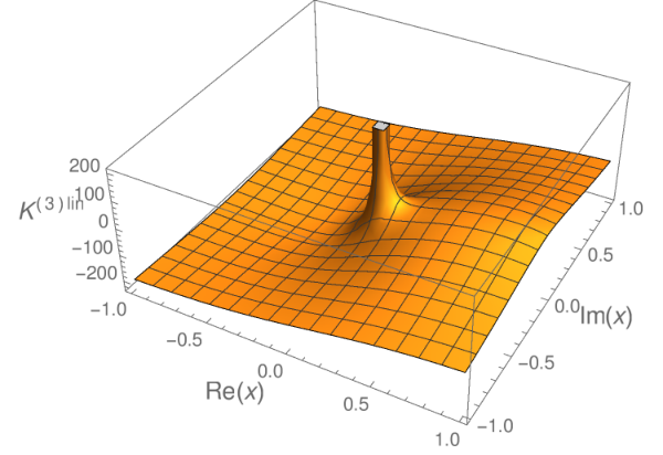
Now the linear equation (77) can be diagonalized explicitly because its eigenfunctions are determined by conformal symmetry [49]. The eigenvalue depends on two quantum numbers: a scaling dimension and an (integer) angular momentum . It can be extracted by looking at the translation invariant wavefunctions55 5 In conventional Regge theory, trajectories are functions of the transverse momentum squared. In a conformal theory there is a continuum of such trajectories for each value of , but this continuum is generated by a symmetry and with fixed and the spectrum becomes discrete, see for example [18].
| (80) |
A special eigenfunction is , corresponding to and , which is a generator of the aforementioned U(1) gauge symmetry at large . The eigenvalue of must thus vanish in this case, which leads to an exact prediction for the intercept of the Odderon trajectory at large [50, 19]:
| (81) |
Since this property was manifest in the original starting point, i.e. eq. (75) before eq. (76) was used, in practice we will use this property to fix the constant . Translation-invariance of the trial wavefunctions enables one transverse integral to be done explicitly. This simplifies the evolution (77) to:
| (82) |
where, labelling four points as , the translation-invariant kernel is
| (83) |
Plugging in the wavefunction (80), we see that the Pomeron trajectory is the Mellin transform of .
The parity symmetry of makes invariant under the inversion . The eigenvalue can thus be written as the sum of two terms, analytic in the lower- and upper-half -planes respectively, representing the contributions from and . Following a common notation in the literature, we thus write the Regge trajectory as:
| (84) |
where, for ,
| (85) |
In summary, the Pomeron trajectory , defined conceptually as the eigenvalue of the evolution (77) on the eigenfunctions (80), is obtained at three loops by computing the Mellin transform (85) of the translation invariant projection (83) of the coordinate space kernel (79).
5.1 Result for the eigenvalue
To efficiently integrate (83) we used the differential equation method, wherein derivatives are iteratively computed and simplified using integration-by-parts identities. This method has a long and successful history in the context of dimensionally regulated Feynman integrals [51, 52]. We used a variant that exploits simplifications occuring for absolutely convergent integrals, based on ideas in refs. [53, 54]. Our procedure is illustrated in appendix B in a few examples. The result is an expression for in terms of iterated integrals starting from the origin .
In principle these iterated integrals could be rewritten in terms of polylogarithms, but we found this neither illuminating nor useful in practice. Rather, to extract the eigenvalue, we found it more efficient to perform the angular integration directly at the level of the iterated integral, using again the differential equation method to obtain the result as a iterated integral in the radial variable . The radial functions then turned out to be conventional harmonic polylogarithms. At one- and two-loop this procedure gives expressions that are very uniform for all transverse angular momentum ():
| (86) | ||||
Here the ‘reg.’ notation is an instruction to subtract all the negative powers of (and powers of they multiply) from the series expansion of the bracket around . The harmonic polylogarithms (with omitted argument ) are defined recursively as [55, 56]66 6 Using classical functions: , and .
| (87) |
The concise expression (86) for the two-loop eigenvalue is apparently new, but we have verified that it agrees, for all values of , with the known result in SYM [10, 11, 57].
Equations (86) takes the form of a Mellin transform over harmonic polylogarithms, which is well-known to give harmonic sums (see appendix C), which in the case of eq. (86) would have argument and . However, it is important to note the “reg” subscript in that equation, which implies that a number of powers of terms, which grows with , have to be subtracted. It would be interesting to see if the result can be usefully written as some kind of “regulated” harmonic sum.
At three-loops, although the “reg.” notation seems to help, we did not succeed in finding a compact formula accounting for the full dependence, and so here we restrict our attention to individual values of , for example
| (88) | |||||
The Mellin integral in eq. (88) gives a practical and efficient way to compute the eigenvalue numerically for any desired value of . The result of the integral can also be formally expressed in terms of harmonic sums (see eq. (106)), although evaluating these sums for complex then requires an analytic continuation. In appendix C we also provide harmonic sums expressions for .
Interestingly, the same constant , fixed here analytically from the condition (81), also appears in the large-spin limit of twist-two anomalous dimensions (), and in the large- limit of the color-adjoint BFKL kernel [58].
A Mathematica notebook trajectories_3loop.nb attached to the arXiv submission article allows to evaluate the eigenvalues for any and . (The command j3Eval[m,nu] evaluates numerically to high accuracy the 3-loop correction to , by numerically integrating the series-expansion around 0 and 1 of the radial functions; the command F3integrandHPL[m] produces symbolic expressions for the radial function and transverse spin in terms of harmonic polylogarithms.)
For even , something new happens: the integrand requires a generalization of harmonic polylogarithms involving iterations of . This is related to the square-root containing entries of the symbol of recorded at the end of appendix B. While still straightforward to evaluate the Mellin transform numerically, the result cannot be written in terms of conventional harmonic sums and it is an interesting open problem to characterize this new class of sums.
Finally, we have compared our result for with the recent works [15, 16], which exploited, respectively, integrability of the theory and high-loop data in the collinear limit. After converting to our basis, we found perfect agreement with both references (showing in particular that they agree with each other). The coordinate space kernel (79), its corresponding eigenvalue for , and the nonlinear terms in eq. (71c), are new predictions.
5.2 Collinear singularities and resummation
The eigenvalue is plotted for and in figs. 5-7. It is apparent that, especially near the peak for , the perturbative series suffers from slow convergence. This was observed already at two loops and explained in terms of nearby singularities in the complex plane at [12].
In short, these singularities are related to the collinear limit of BFKL, where the scaling dimension of the exchanged state coincides with that of twist-two operators: with close to 1, e.g. the operators entering the DGLAP equation. As is common for two-level quantum systems, this crossing of two energy levels [18] gets resolved as depicted in fig. 6:
| (89) |
At small , one branch choice gives the near-horizontal BFKL trajectory while the other gives the 45∘ twist-two (DGLAP) trajectory. (The square root formula follows easily by solving for the , within the overlapping regime of validity of BFKL and DGLAP where the anomalous dimension can be approximated by its leading pole.) It was shown that, expanding the square root to order , reduces by half the magnitude of the two-loop corrections to the intercept (if one also includes the complex conjugate singularity at ) [12]. The “LO resummation” curve in fig. 5, called “scheme 2” in ref. [12], thus shows the LO trajectory plus eq. (89) minus its expansion. (It would be useful to develop a NLO resummation and we leave it as an open problem for the future.)
The formula (89), expanded to three loops, turns out to not predict very well the three-loop correction to the intercept . In fact it gets even the sign wrong. By looking at the singular terms in close to the pole we can try to understand why:
| (90) |
where . Comparing with eq. (89), we find that the leading pole is exactly as predicted (as it had to). Setting , the subleading poles however also give a numerically large contribution to the intercept , so truncating to the leading pole does not give a good approximation to the intercept. However, summing up all the singular terms in eq. (90), one finds that about of the three-loop correction to the intercept is reproduced. A heuristic explanation is that the contributions from the next singularities, at , are suppressed by their distance.
Interestingly, all polar terms at -loops can be obtained from the -loop DGLAP equation. (See for example [59, 60].) From the higher-loop DGLAP equation one can get nonsingular terms in the expansion (90), see for example eq. (21) of [16]. We have verified that our result (88-106) agrees with all these constraints.77 7 Compared to eq. (21) of [16] (version 1), we have , to match with the generally accepted convention that we are following.
We conclude that the physical picture of [12], that large corrections to the intercept originate from the collinear singularities, is consistent with the three-loop trajectory we obtained, although the full polar part, predicted by DGLAP (as opposed to just the leading pole), must be retained. In general it would be very interesting to find a way to make full use of the DGLAP information at a given loop order
Finally, we comment on the Mellin transform of the level-crossing formula (89) back to coordinate space. The transform produces a Bessel function:
| (91) |
The right-hand side has appeared in coordinate space and momentum space resummations [13, 14], so it is nice to see how it arises form the familiar two-level crossing formula (89).
6 Discussion and conclusion
In this paper we have computed, for the first time, the evolution equation which resums large rapidity logarithms in forward scattering to three loops in a gauge theory. Our main results are the full nonlinear equation (71) in planar supersymmetric Yang-Mills theory, its linearization (79), characterizing the BFKL Pomeron in impact parameter space, as well as its eigenvalue, the Pomeron Regge trajectory, described in appendix C. This result is a first step toward the analogous QCD result, and by itself can already be used to assess the convergence of perturbation theory and its proposed resummations, and shed light on nonlinear saturation effects at finite coupling.
This computation was made possible thanks to a recently established correspondence with the resummation of large so-called non-global logarithms, which occur when soft radiation is excluded from a fixed angular region. This correspondence is helpful because it makes available a body of knowledge on the factorization of infrared and collinear divergences, and at a conceptual level it defines in a clear way the evolution equation to all loop orders. This allowed us to derive a systematic subtraction method for nested subdivergences, embodied in eq. (55), such that all energy integrals at fixed angle become convergent. We then dealt with collinear subdivergences and real-virtual cancellations in a second step, by multiplying and dividing by the corrections to the single soft current as in eq. (48).
Therefore, although we set up our calculation in dimensional regularization and some divergent intermediate objects appeared, we find that in the end the evolution equation depends only on the limit of physical scheme-independent quantities like the the Bern-Dixon-Smirnov remainder (50)! This opens a new possibility to relate an object with the topology of the cylinder, the BFKL Pomeron, to the integrable system appearing in planar scattering amplitudes [61]; graphically speaking, this cuts the cylinder into two half-pipes.
As a highly nontrivial test, of both our calculation and of the integrability approach, we have compared our extracted Pomeron trajectory (88) with the recent predictions for in [15, 16], and found perfect agreement! We have also found perfect agreement, in the collinear limit, with the prediction from anomalous dimensions of twist-two operators. The trajectory for other transverse angular momenta , and nonlinear interactions, are new predictions which it would be very interesting to check within the integrability approach.
It is important to clarify the counting in which our result is valid. The projectile is assumed to be made of a finite number of Wilson lines, but whose expectation values across the target can be finite, . This asymmetric setup, motivated for example in proton-nucleus collisions, is the same as that for which the Balitsky-Kovchegov equation is strictly derived. In the context of AdS/CFT this counting would apply to e.g. a light probe of a black hole. This is also a well-defined setup and in fact it would be interesting to work out the nonlinear terms in the Balitsky-Kovchegov equation at strong coupling , including perhaps stringy effects. The linear terms, which govern correlators of light operators with large but not-to-large energies (before the onset of saturation, such that ) have already been identified with graviton exchange [18].
There are several directions in which this work could be extended. One is to go beyond the planar limit at weak coupling, where the two-loop corrections have recently become available [62, 63, 23]. Interesting new physical effects appear at three loops in the non-planar sector, for example the reggeon transition which “closes the Pomeron loop” and restores the symmetry between the target and projectile would first be seen there (see for example [19]). Through the KLN theorem, the three-loop evolution could also independently predict from real corrections, and thus test, the recent result for three-loop soft anomalous dimension [64]. Another direction is towards QCD: technically, our setup gives direct access to the evolution equation for non-global logarithms, which in QCD will differ from rapidity evolution by terms proportional to the -function. These could thus be calculated subsequently by calculating matter loops on both sides of the correspondence.
Acknowledgements.
SCH would like to thank Kolya Gromov and Vitaly Velizhanin for discussions regarding the integrability prediction for the trajectory. SCH’s work was supported partly by the Danish FNU Grant No. 126152 and by the Danish National Research Foundation (DNRF91). MH is supported by the Villum Foundation Grant No. YIP/VKR022599.Appendix A One-loop correction to the squared double soft current
Here we record the interference of the tree and one-loop double soft current, defined in eq. (42), obtained from the soft limit of the six point amplitude as explained in the text.
| (92) | |||||
with , and the parity operation : . Here all analytic continuations have been performed, so the logarithms are all real for timelike (positive) invariants, as is the case for our application. The infrared divergences are contained in the factor but in practice all we will need is the fully renormalized form factor, defined in eq. (48), which is finite and obtained by a simple substitution:
| (93) |
Appendix B Doing transverse integrals efficiently
Two-dimensional integrals can be done extremely efficiently with the differential equation method. Here we elaborate on our implementation, emphasizing the simplifications related to the fact that all the integrals are absolutely convergent and done directly in dimensions. We first illustrate the method on the integral
| (94) |
which occurs at two-loops when obtaining the translation-invariant kernel (83). The idea is to differentiate with respect to and add a total derivative with respect to to remove derivatives of rational factors. Indeed, using the relevant identity:
| (95) |
one readily gets that
| (96) |
We “win” because the derivatives commutes with the rational factor and hits the logarithm, producing a simpler integral.
An important subtlety is that the left-hand-side of eq. (95) is singular and so the equation is only strictly valid for generic . There are additional contact terms given by the “holomorphic anomaly”
| (97) |
This can be understood from the two-dimensional Poisson equation . These terms would be absent in dimensional regularization but appear because we insist to work with (see [54] for four-dimensional examples). In the example (96), the contact terms are at and but the logarithm turns out to vanish on both, so these can be dropped. Evaluating the derivative then gives simply
| (98) |
To finish, one can repeat the same procedure, inserting a variant of eq. (95) to differentiate the integral with respect to (and/or ). Now only the contact term contributes and a general result obtained this way is
| (99) |
which gives (using the vanishing at to fix the integration constant)
| (100) |
This result can be easily confirmed by numerical integration.
A critical point to emphasize is that the factor in eq. (98) had to be pulled out in front of the integral before taking the second derivative. If the derivative were allowed to act on that factor, one would gain nothing from it. Only properly normalized integrals simplify upon taking derivatives.
A simple criterion to identify properly normalized integrals is that all the Poincaré residues of their rational factors should be constant (these are often called leading singularities). These are simply the double residue with respect to followed by , of the rational factors in the integrand, with and treated as independent complex variables. This property is easily verified in eqs. (94) and (99). Its significance is that it ensures that derivatives of the rational factors have vanishing Poincaré residues, which is needed for them to be total derivatives which simplify upon integration by parts as in eq. (95). See for instance refs. [53, 54] for other applications of this criterion.
The procedure to decompose an integral into properly normalized ones is essentially partial fractions. When the denominators do not couple and , it is in fact literally partial fraction in these two variables, one after the other. But the integrals we need also contain in the denominator an irreducible quadratic form , which is harder to partial-fraction out. We illustrate this with the other integral appearing in , coming from the second term in the kernel (22):
Despite appearances, is a quadratic form in . The leading singularities of the rational factor can be computed and found to be linear combinations of and , so the decomposition into properly normalized integrals will require two terms. To illustrate the result of the partial-fraction method to be detailed shortly, one indeed finds that the integral can be rewritten exactly as:
| (101) |
This rewriting of the integrand is a purely algebraic identity. The upshot is that all residues have been pulled out and the leading singularities of the rational factor inside the integral are only . One then expects, and finds, that the derivative of the integral is a total derivatives in and . One does not need to make any clever guess to find this total derivatives: in practice we simply write down an ansatz with a polynomial numerator in and and solve for the coefficients. We obtain for example the identity:
again up to contact terms arising from the holomorphic anomaly (at and ). Plugging this into the integral (101) thus gives its -derivative in terms of contact terms and the simpler integral (99). The derivative can then be easily integrated, and the integration constant again is fixed by the vanishing at , yielding the two-loop linearized kernel:
| (102) |
This agrees precisely with the result in eq. (105) of Balitsky& Chirilli 0710.4330.
Chief advantages of this method are its speed and uniform applicability. Indeed, the basic steps (integration by parts and partial fractions) are algebraic and independent of the transcendental weight of the functions being integrated. That is, the same code we used to do the two-loop integral as just described, automatically also worked for and would presumably work at higher orders as well (producing the result as an iterated integral).
To conclude, we elaborate on partial fractions in the presence of the quadratic form in the denominator. The main step is to exploit the geometry to create a complete basis. For the integrals involving , there are other singularities on the 8 lines and , each line intersecting the quadric at two points. However the geometry is a bit degenerate and there are only 8 intersections: . A complete basis of rational functions is then obtained by writing 8 objects where and the numerators are linear in and chosen to leave only one Poincaré residue nonzero (and equal to 1). A ninth integral (accounting for a residue at infinity), together with simpler integrals with only linear denominators, complete the basis. Once a basis is fixed, partial fraction identities like (101) follow simply from computing Poincaré residues, a fast operation.
The other integrals needed in this paper, involving the triple-real functions (70) and (78), were dealt with in a similar way, although their geometry is somewhat simpler (no square roots appeared in these cases).
B.1 Single-valued functions for the linearized kernel
The linearized kernel (78) is a weight 3 function of one complex variable; the preceding method produces it in the form of an iterated integral, whose integration constants could be easily fixed from the limit . Its symbol turns out to be made of the five letters and . At transcendental weight 3, we found only three nontrivial single-valued functions with such symbol, in terms of which the three-loop linearized kernel in (79) is compactly written:
| (103a) | |||||
| (103b) | |||||
| (103c) | |||||
Although not manifest from these formulas, these functions have no branch cut on the complex plane where . This can be confirmed by series-expanding around singular points such as and , where to all orders one finds only single-valued logarithms of or but never nor separately. Furthermore, there are no singularities along (which traces a unit circle with center at ).
We note that the same five letters are also singularities of the two-loop kernel, so it is natural to conjecture that no other letters appear in to any order in perturbation theory in planar SYM. Its translation-invariant projection , defined by the integration (83), can then be obtained by applying the algorithm detailed above, which implies that at most the ten letters , can appear in its symbol (all of which do indeed appear at three loops).
Appendix C Eigenvalue in terms of harmonic sums for and
Here we give explicit expressions for the 3-loop Pomeron trajectory, given in coordinate space in eq. (79), in Mellin space using the harmonic sums
| (104) |
This defines the sums for integer and the Mellin transform produces their analytical continuation from even . Using standard algorithms [55], we have converted the Mellin integral projected onto transverse angular momentum , eq. (88), to harmonic sums with argument :
| (105) | |||||
| (106) | |||||
Here and are multi-zeta values. This result is in precise agreement with [15]. The Pomeron trajectory is the sum of and , see eq. (84). For our result is new. For , for example, the Mellin transform can be expressed in terms of harmonic sums now with argument , giving the Odderon Regge trajectory:
| (107) | |||||
| (108) | |||||
This is regular and in fact vanishes at , in accordance with the all-order result (81). Other values of can be evaluated numerically using the attached Mathematica notebook.
References
- (1) E. Kuraev, L. Lipatov, and V. S. Fadin, The Pomeranchuk Singularity in Nonabelian Gauge Theories, Sov.Phys.JETP 45 (1977) 199–204.
- (2) I. Balitsky and L. Lipatov, The Pomeranchuk Singularity in Quantum Chromodynamics, Sov.J.Nucl.Phys. 28 (1978) 822–829.
- (3) I. Balitsky, Operator expansion for high-energy scattering, Nucl.Phys. B463 (1996) 99–160, [hep-ph/9509348].
- (4) Y. V. Kovchegov, Small x F(2) structure function of a nucleus including multiple pomeron exchanges, Phys.Rev. D60 (1999) 034008, [hep-ph/9901281].
- (5) L. D. McLerran and R. Venugopalan, Computing quark and gluon distribution functions for very large nuclei, Phys. Rev. D49 (1994) 2233–2241, [hep-ph/9309289].
- (6) F. Gelis, E. Iancu, J. Jalilian-Marian, and R. Venugopalan, The Color Glass Condensate, Ann. Rev. Nucl. Part. Sci. 60 (2010) 463–489, [arXiv:1002.0333].
- (7) F. Caporale, G. Chachamis, B. Murdaca, and A. S. Vera, Balitsky-Fadin-Kuraev-Lipatov Predictions for Inclusive Three Jet Production at the LHC, Phys. Rev. Lett. 116 (2016), no. 1 012001, [arXiv:1508.0771].
- (8) E. Iancu, J. D. Madrigal, A. H. Mueller, G. Soyez, and D. N. Triantafyllopoulos, Collinearly-improved BK evolution meets the HERA data, Phys. Lett. B750 (2015) 643–652, [arXiv:1507.0365].
- (9) I. Balitsky and G. A. Chirilli, Next-to-leading order evolution of color dipoles, Phys.Rev. D77 (2008) 014019, [arXiv:0710.4330].
- (10) V. S. Fadin and L. Lipatov, BFKL pomeron in the next-to-leading approximation, Phys.Lett. B429 (1998) 127–134, [hep-ph/9802290].
- (11) M. Ciafaloni and G. Camici, Energy scale(s) and next-to-leading BFKL equation, Phys. Lett. B430 (1998) 349–354, [hep-ph/9803389].
- (12) G. P. Salam, A Resummation of large subleading corrections at small x, JHEP 07 (1998) 019, [hep-ph/9806482].
- (13) A. Sabio Vera, An ’All-poles’ approximation to collinear resummations in the Regge limit of perturbative QCD, Nucl. Phys. B722 (2005) 65–80, [hep-ph/0505128].
- (14) E. Iancu, J. D. Madrigal, A. H. Mueller, G. Soyez, and D. N. Triantafyllopoulos, Resumming double logarithms in the QCD evolution of color dipoles, Phys. Lett. B744 (2015) 293–302, [arXiv:1502.0564].
- (15) N. Gromov, F. Levkovich-Maslyuk, and G. Sizov, Pomeron Eigenvalue at Three Loops in 4 Supersymmetric Yang-Mills Theory, Phys. Rev. Lett. 115 (2015), no. 25 251601, [arXiv:1507.0401].
- (16) V. N. Velizhanin, BFKL pomeron in the next-to-next-to-leading approximation in the planar N=4 SYM theory, arXiv:1508.0285.
- (17) I. Balitsky, V. Kazakov, and E. Sobko, Three-point correlator of twist-2 operators in BFKL limit, arXiv:1506.0203.
- (18) R. C. Brower, J. Polchinski, M. J. Strassler, and C.-I. Tan, The Pomeron and gauge/string duality, JHEP 0712 (2007) 005, [hep-th/0603115].
- (19) S. Caron-Huot, When does the gluon reggeize?, JHEP 05 (2015) 093, [arXiv:1309.6521].
- (20) A. Banfi, G. Marchesini, and G. Smye, Away from jet energy flow, JHEP 08 (2002) 006, [hep-ph/0206076].
- (21) G. Marchesini and A. H. Mueller, The BMS Equation and Production; A Comparison of the BMS and BK Equations, JHEP 02 (2016) 010, [arXiv:1510.0876].
- (22) Y. Hatta, Relating e+ e- annihilation to high energy scattering at weak and strong coupling, JHEP 0811 (2008) 057, [arXiv:0810.0889].
- (23) S. Caron-Huot, Resummation of non-global logarithms and the BFKL equation, arXiv:1501.0375.
- (24) D. M. Hofman and J. Maldacena, Conformal collider physics: Energy and charge correlations, JHEP 0805 (2008) 012, [arXiv:0803.1467].
- (25) L. Cornalba, M. S. Costa, and J. Penedones, Deep Inelastic Scattering in Conformal QCD, JHEP 03 (2010) 133, [arXiv:0911.0043].
- (26) H. Weigert, Nonglobal jet evolution at finite N(c), Nucl. Phys. B685 (2004) 321–350, [hep-ph/0312050].
- (27) Z. Nagy and D. E. Soper, Parton shower evolution with subleading color, JHEP 1206 (2012) 044, [arXiv:1202.4496].
- (28) A. J. Larkoski, I. Moult, and D. Neill, Non-Global Logarithms, Factorization, and the Soft Substructure of Jets, JHEP 09 (2015) 143, [arXiv:1501.0459].
- (29) T. Becher, M. Neubert, L. Rothen, and D. Y. Shao, Effective Field Theory for Jet Processes, Phys. Rev. Lett. 116 (2016), no. 19 192001, [arXiv:1508.0664].
- (30) S. Catani and M. Grazzini, Infrared factorization of tree level QCD amplitudes at the next-to-next-to-leading order and beyond, Nucl.Phys. B570 (2000) 287–325, [hep-ph/9908523].
- (31) I. Feige and M. D. Schwartz, Hard-Soft-Collinear Factorization to All Orders, Phys.Rev. D90 (2014), no. 10 105020, [arXiv:1403.6472].
- (32) I. Balitsky and G. A. Chirilli, NLO evolution of color dipoles in N=4 SYM, Nucl.Phys. B822 (2009) 45–87, [arXiv:0903.5326].
- (33) E. Avsar, Y. Hatta, and T. Matsuo, Soft gluons away from jets: Distribution and correlation, JHEP 0906 (2009) 011, [arXiv:0903.4285].
- (34) R. Ángeles Martínez, J. R. Forshaw, and M. H. Seymour, Ordering multiple soft gluon emissions, Phys. Rev. Lett. 116 (2016), no. 21 212003, [arXiv:1602.0062].
- (35) T. Kinoshita, Mass singularities of Feynman amplitudes, J.Math.Phys. 3 (1962) 650–677.
- (36) T. Lee and M. Nauenberg, Degenerate Systems and Mass Singularities, Phys.Rev. 133 (1964) B1549–B1562.
- (37) Z. Bern, V. Del Duca, W. B. Kilgore, and C. R. Schmidt, The infrared behavior of one loop QCD amplitudes at next-to-next-to leading order, Phys.Rev. D60 (1999) 116001, [hep-ph/9903516].
- (38) S. Catani and M. Grazzini, The soft gluon current at one loop order, Nucl.Phys. B591 (2000) 435–454, [hep-ph/0007142].
- (39) Z. Bern, J. S. Rozowsky, and B. Yan, Two loop four gluon amplitudes in N=4 superYang-Mills, Phys. Lett. B401 (1997) 273–282, [hep-ph/9702424].
- (40) J. L. Bourjaily, A. DiRe, A. Shaikh, M. Spradlin, and A. Volovich, The Soft-Collinear Bootstrap: N=4 Yang-Mills Amplitudes at Six and Seven Loops, JHEP 03 (2012) 032, [arXiv:1112.6432].
- (41) J. L. Bourjaily, P. Heslop, and V.-V. Tran, Perturbation Theory at Eight Loops: Novel Structures and the Breakdown of Manifest Conformality, arXiv:1512.0791.
- (42) J. L. Bourjaily, Efficient Tree-Amplitudes in N=4: Automatic BCFW Recursion in Mathematica, arXiv:1011.2447.
- (43) Z. Bern, L. J. Dixon, D. C. Dunbar, and D. A. Kosower, One loop n point gauge theory amplitudes, unitarity and collinear limits, Nucl. Phys. B425 (1994) 217–260, [hep-ph/9403226].
- (44) Z. Bern, L. J. Dixon, D. C. Dunbar, and D. A. Kosower, Fusing gauge theory tree amplitudes into loop amplitudes, Nucl. Phys. B435 (1995) 59–101, [hep-ph/9409265].
- (45) J. M. Drummond, J. Henn, G. P. Korchemsky, and E. Sokatchev, Dual superconformal symmetry of scattering amplitudes in N=4 super-Yang-Mills theory, Nucl. Phys. B828 (2010) 317–374, [arXiv:0807.1095].
- (46) J. L. Bourjaily, S. Caron-Huot, and J. Trnka, Dual-Conformal Regularization of Infrared Loop Divergences and the Chiral Box Expansion, JHEP 01 (2015) 001, [arXiv:1303.4734].
- (47) Z. Bern, L. J. Dixon, and V. A. Smirnov, Iteration of planar amplitudes in maximally supersymmetric Yang-Mills theory at three loops and beyond, Phys.Rev. D72 (2005) 085001, [hep-th/0505205].
- (48) N. Beisert, B. Eden, and M. Staudacher, Transcendentality and Crossing, J.Stat.Mech. 0701 (2007) P01021, [hep-th/0610251].
- (49) L. Lipatov, The Bare Pomeron in Quantum Chromodynamics, Sov.Phys.JETP 63 (1986) 904–912.
- (50) Y. V. Kovchegov, Running Coupling Evolution for Diffractive Dissociation and the NLO Odderon Intercept, AIP Conf.Proc. 1523 (2012) 335–338, [arXiv:1212.2113].
- (51) A. V. Kotikov, Differential equations method: New technique for massive Feynman diagrams calculation, Phys. Lett. B254 (1991) 158–164.
- (52) T. Gehrmann and E. Remiddi, Differential equations for two loop four point functions, Nucl. Phys. B580 (2000) 485–518, [hep-ph/9912329].
- (53) J. M. Henn, Multiloop integrals in dimensional regularization made simple, Phys. Rev. Lett. 110 (2013) 251601, [arXiv:1304.1806].
- (54) S. Caron-Huot and J. M. Henn, Iterative structure of finite loop integrals, JHEP 06 (2014) 114, [arXiv:1404.2922].
- (55) E. Remiddi and J. A. M. Vermaseren, Harmonic polylogarithms, Int. J. Mod. Phys. A15 (2000) 725–754, [hep-ph/9905237].
- (56) D. Maitre, HPL, a mathematica implementation of the harmonic polylogarithms, Comput. Phys. Commun. 174 (2006) 222–240, [hep-ph/0507152].
- (57) A. V. Kotikov and L. N. Lipatov, DGLAP and BFKL equations in the N=4 supersymmetric gauge theory, Nucl. Phys. B661 (2003) 19–61, [hep-ph/0208220]. [Erratum: Nucl. Phys.B685,405(2004)].
- (58) B. Basso, S. Caron-Huot, and A. Sever, Adjoint BFKL at finite coupling: a short-cut from the collinear limit, JHEP 01 (2015) 027, [arXiv:1407.3766].
- (59) S. Marzani, R. D. Ball, P. Falgari, and S. Forte, BFKL at next-to-next-to-leading order, Nucl. Phys. B783 (2007) 143–175, [arXiv:0704.2404].
- (60) M. S. Costa, V. Goncalves, and J. Penedones, Conformal Regge theory, JHEP 12 (2012) 091, [arXiv:1209.4355].
- (61) B. Basso, A. Sever, and P. Vieira, Hexagonal Wilson Loops in Planar SYM Theory at Finite Coupling, arXiv:1508.0304.
- (62) I. Balitsky and G. A. Chirilli, Rapidity evolution of Wilson lines at the next-to-leading order, Phys.Rev. D88 (2013) 111501, [arXiv:1309.7644].
- (63) A. Kovner, M. Lublinsky, and Y. Mulian, Jalilian-Marian, Iancu, McLerran, Weigert, Leonidov, Kovner evolution at next to leading order, Phys.Rev. D89 (2014) 061704, [arXiv:1310.0378].
- (64) Ø. Almelid, C. Duhr, and E. Gardi, Three-loop corrections to the soft anomalous dimension in multi-leg scattering, arXiv:1507.0004.