跳到论文正文
W Papers独立论文阅读器 arXiv:1604.07303 论文正文 计算阅读时间 · 0%
引用这篇论文根据当前论文元数据生成,正式投稿前建议核对。


License: arXiv.org perpetual non-exclusive license
arXiv:1604.07303v2 [math.DG] 03 Jul 2016

On approximation of planar curves by circular arcs with length preservation

Alexey Kurnosenko
Abstract

The method for approximation of a planar curve by circular arcs with length preservation, proposed by I. Kh. Sabitov and A. V. Slovesnov, is analyzed. We extend the applicability of the method, and consider some corollaries, not related to the approximation problem. Inequalities for the length of a convex spiral arc with prescribed two-point G1 or G2 Hermite data are derived. We propose a scheme of computer modelling to explore properties of planar curves. As an example, closeness of ovals is tested, leading to some conjectures about closeness conditions.


Keywords: spiral curve, biarc, bilens, triarc, curves approximation, length preservation, cochleoid, cycloidal curves, closed curves.

This note further develops the subject of article [1], whose motivation is sufficiently reasoned by the authors. In [1] a segment of monotone curvature within some given curve is approximated by a biarc curve, sharing end points and end tangents with the segment. In Computer-Aided Design (CAD) applications this is a well-known problem of approximation with given two-point G1 Hermite data. Additional condition is required to select a solution among a family of biarcs. E. g., the condition of minimal curvature jump in the join point could be imposed. To the author’s knowledge, the condition of lengths preservation, proposed in [1], is new for this problem.

Here we extend both the variety of curves, to which the method could be applied (see comments to Theorem 1), and fields of its application, not related to the approximation problem (Sections 3, 4). First, we precise some terminology.

  • •

    As the customary to CAD, we designate curves with monotone curvature as spirals [2].

  • •

    Biarc curve [2, 3] is the curve, composed of two non-closed circular (linear) arcs.

  • •

    Triarc curve is composed of three circular arcs. Curvatures k1,k2,k3k_{1},k_{2},k_{3} of a spiral triarc form a monotone sequence.

1 Notation and some properties of biarcs

Let [x⁡(s),y⁡(s)][x(s),y(s)] be a planar curve, parametrized by the arc length ss. The curvature at a point is defined by derivative k⁡(s)=τs′k(s)=\tau^{\prime}_{s}, where τ⁡(s)=arg⁡(xs′+i​ys′)\tau(s)=\arg(x^{\prime}_{s}+{\mathrm{i}}y^{\prime}_{s}). Curvature element 𝒦0={x0,y0,τ0,k0}{{\mathcal{K}_{0}}}=\left\{x_{0},y_{0},\tau_{0},k_{0}\right\} at the point (x0,y0)(x_{0},y_{0}) includes the slope τ0\tau_{0} of the tangent vector 𝐧⁡(τ0)=(cos⁡τ0,sin⁡τ0)\mathbf{n}\left(\tau_{0}\right)=(\cos\tau_{0},\,\sin\tau_{0}), and curvature k0k_{0}, thus defining the directed circle of curvature at this point.

A spiral arc A​B⌢\displaystyle{\mathrel{\mathop{\kern 0.0ptAB}\limits^{\,\,\frown}}}, supported by the chord of the length |A​B|=2​c\left\lvert AB\right\rvert=2c, is considered in the local coordinate system with point AA moved to position (−c,0)(-c,0), and BB to (c,0)(c,0). Boundary curvature elements are

𝒦1={−c,0,α,k1},𝒦2={c,0,β,k2};denote alsoγ=α−β2,ω=α+β2.{{\mathcal{K}_{1}}}=\left\{-c,0,\alpha,k_{1}\right\},\quad{{\mathcal{K}_{2}}}=\left\{c,0,\beta,k_{2}\right\};\quad\text{denote also}\quad\gamma=\frac{\alpha-\beta}{2},\quad\omega=\frac{\alpha+\beta}{2}\,. (1)

In Fig. 1a two spiral arcs with boundary data (1) are shown by dotted lines; the example to the left presents a convex curve, the rightward one shows a curve with inflection. Three circular arcs are traced from start point AA to end point BB of each curve. One of them shares tangent 𝐧⁡(α)\mathbf{n}\left(\alpha\right) with the spiral at AA, the other shares tangent 𝐧⁡(β)\mathbf{n}\left(\beta\right) at BB. These two arcs form the lens. The third circular arc, shown dotted-dashed, traced from AA at the angle γ\gamma, is the bisector of the lens ; ω\omega is the angular half-width of the lens.

In [4] the inversive invariant QQ of a pair of circles was proposed, equal to sin2⁡Ψ2\sin^{2}\frac{\Psi}{2}, where Ψ\Psi is intersection angle of two circles (purely imaginary if Q<0Q<0). For pair (1)

Q=(k1​c+sin⁡α)​(k2​c−sin⁡β)+sin2⁡ω.Q=(k_{1}c+\sin\alpha)(k_{2}c-\sin\beta)+\sin^{2}\omega. (2)

According to [2] (theorem 2), Q<0Q<0 is the necessary and sufficient condition for existence of a non-biarc spiral with two-point G2 Hermite data (1). If Q=0Q=0, boundary circles of curvature are tangent, and the only possible spiral in this case is biarc.

1.1 Short spirals

We call a spiral arc A​B⌢\displaystyle{\mathrel{\mathop{\kern 0.0ptAB}\limits^{\,\,\frown}}} short, if it has no common points with its chord’s complement to the infinite straight line (possibly, intersecting the chord itself). In [1] „very short spirals“ are considered, namely, those, one-to-one projectable onto the chord.

  • •

    Existence conditions for a short non-biarc spiral with two-point G2 Hermite data (1) are: Q<0Q<0, and

    if ​k1<k2:−π<α⩽π,−π<β⩽π,α+β>0;if ​k1>k2:−π⩽α<π,−π⩽β<π,α+β<0\begin{array}[]{llll}\text{if\penalty\ \penalty\ }k_{1}<k_{2}{:}&-\pi<\alpha\leqslant\pi,&-\pi<\beta\leqslant\pi,&\alpha+\beta>0;\\ \text{if\penalty\ \penalty\ }k_{1}>k_{2}{:}&-\pi\leqslant\alpha<\pi,&-\pi\leqslant\beta<\pi,&\alpha+\beta<0\end{array} (3)

    [5, theorems 1, 3]. The choice between ±π\pm\pi is imposed by continuity of function τ⁡(s)\tau(s), whose values in internal points of a short spiral are in the interval (−π,π)(-\pi;\pi). E. g., spiral with α=β=−π\alpha=\beta=-\pi looks like [Uncaptioned image].

  • •

    Existence conditions for a short biarc with two-point G2 Hermite data (1) require Q=0Q=0 and, additionally to (3), |α+β|≠2​π\left\lvert\alpha+\beta\right\rvert\neq 2\pi. This excludes cases α=β=±π\alpha=\beta=\pm\pi.

  • •

    Conditions (3) include Vogt’s theorem (see [5], theorem 1 and references):

    ⁡s​g​n​(k2−k1)=⁡s​g​n​(α+β).\mathop{\mathrm{}}{sgn}\nolimits(k_{2}-k_{1})=\mathop{\mathrm{}}{sgn}\nolimits(\alpha+\beta).\vskip-3.60004pt (4)

    The theorem remains valid for long spirals, if the values of boundary angles are uniquely precised as α→α+2​m​π\alpha\to\alpha{+}2m\pi, β→β+2​n​π\beta\to\beta{+}2n\pi, to become „the angles, bearing their history“.

  • •

    Short spiral is enclosed into the lens [5, theorem 2].

Refer to caption
Figure 1: (a) Spiral arc (traced by dotted line), its boundary tangents, and the lens; the left example is for 0⩽k1<k20\leqslant k_{1}<k_{2}, and the right one for k1<0<k2k_{1}<0<k_{2}; (b) a family of short biarcs, filling the lens; examples of long biarcs are shown dashed; (c) boundary circles of curvature of the spiral arcs (dashed), defining bilens.

1.2 A family of biarcs with common end tangents

In Fig. 1b the lens is filled with the family of short biarcs, having common end tangents 𝐧⁡(α)\mathbf{n}\left(\alpha\right), 𝐧⁡(β)\mathbf{n}\left(\beta\right). Join points JJ are marked by arrows. Dashed curves show some examples of long biarcs.

Applying homothety with scale factor c−1c^{-1} causes transformations

A→(−1,0),B→(1,0),α→α,β→β,k1→a=k1​c,k2→b=k2​c.A\to(-1,0),\quad B\to(1,0),\quad\alpha\to\alpha,\quad\beta\to\beta,\quad k_{1}\to a=k_{1}c,\quad k_{2}\to b=k_{2}c.

The values aa and bb become dimensionless curvatures of arcs A​JAJ and J​BJB, normalized to the chord length 2​c=22c=2. The condition of tangency of these two arcs, Q=0Q=0, looks like

Q⁡(a,b)=0,whereQ⁡(a,b)=(2)(a+sin⁡α)​(b−sin⁡β)+sin2⁡ω.Q(a,b)=0,\quad\text{where}\quad Q(a,b)\mathrel{\mathop{\kern 0.0pt=}\limits^{\eqref{DefQ1}}}(a+\sin\alpha)(b-\sin\beta)+\sin^{2}\omega. (5)

In the curvatures plane (a;b)(a;b) the curve Q⁡(a,b)=0Q(a,b)=0 is the hyperbola, shown in Fig. 2. Its possible parametrizations [a⁡(p),b⁡(p)][a(p),\,b(p)] yield the parametrization of the biarcs family under consideration. As in [6], we accept

kA​J=a⁡(p)c,kJ​B=b⁡(p)c,wherea(p)=−sinα−sin⁡ωp,b(p)=sinβ+psinω.k_{AJ}=\frac{a(p)}{c},\quad k_{JB}=\frac{b(p)}{c},\quad\text{where}\quad a(p)=-\sin\alpha-\frac{\sin\omega}{p},\quad b(p)=\sin\beta+p\,\sin\omega. (6)

Under such parametrization biarcs with p>0p>0 are short [6], Proof of Property 3). Some properties of biarcs ℬ⁡(p,α,β)\mathcal{B}(p;\alpha,\beta) are mentioned here as functions of family parameter pp.

Join points (XJ,YJ)(X_{J},Y_{J}) form a circular arc ([6, Property 6])

XJ​(p,γ)+i​YJ​(p,γ)=c​p2−1+2​i​p​sin⁡γp2+2​p​cos⁡γ+1.X_{J}(p;\gamma)+{\mathrm{i}}Y_{J}(p;\gamma)=c\,\frac{p^{2}{-}1+2{\mathrm{i}}p\sin\gamma}{{p^{2}+2p\cos\gamma+1}}.

Its arc 0⩽p⩽∞0\leqslant p\leqslant\infty is the lens’ bisector, the locus of join points of short biarcs.

The total turning of a short biarc is equal to β−α\beta-\alpha (and β−α±2​π\beta-\alpha\pm 2\pi for a long one). It is the sum of turnings θ1,2\theta_{1,2} of each subarc [6, Property 9]:

θ1(p)=τJ(p)−α,θ2(p)=β−τJ(p),τJ(p)=−2arctanp​sin⁡α2+sin⁡β2p​cos⁡α2+cos⁡β2=−ω+2arctan(1−p1+p⋅tanγ2)\begin{array}[]{l}\theta_{1}(p)=\tau_{{}_{J}}(p)-\alpha,\\ \theta_{2}(p)=\beta-\tau_{{}_{J}}(p),\end{array}\quad\tau_{{}_{J}}(p)={-2}\arctan\dfrac{p\sin\frac{\alpha}{2}+\sin\frac{\beta}{2}}{p\cos\frac{\alpha}{2}+\cos\frac{\beta}{2}}=-\omega+2\arctan\left(\dfrac{1-p}{1+p}\cdot\tan\dfrac{\gamma}{2}\right) (7)

(with no ±2​π\pm 2\pi corrections for short biarcs). The angle τJ\tau_{{}_{J}} is the slope of tangent to a biarc at the join point. The length S⁡(p)S(p) of a biarc is

S⁡(p)=S1​(p)+S2​(p), where ​S1​(p)=c​θ1​(p)a⁡(p),S2​(p)=c​θ2​(p)b⁡(p).S(p)=S_{1}(p)+S_{2}(p),\text{\penalty\ \penalty\ where\penalty\ \penalty\ }S_{1}(p)=c\frac{\theta_{1}(p)}{a(p)},\quad S_{2}(p)=c\frac{\theta_{2}(p)}{b(p)}. (8)

The length S⁡(p)S(p) of a short biarc is a strictly monotone function of parameter pp, or constant, if α=β\alpha=\beta [6, Property 11]. Let us precise the type of monotonicity of S⁡(p)S(p) (not specified in [6]) by looking at limit cases p→0p\to 0 and p→+∞p\to{+\infty}. If p→0p\to 0, the join point J⁡(p)J(p) of biarc A​J​BAJB tends to point AA, arc A​JAJ vanishes, and the biarc degenerates to the circular arc, one of lens boundaries, the lower one under conditions of Fig. 1. If p→∞p\to\infty, J⁡(p)→BJ(p)\to B, biarc A​J​BAJB degenerates to the second lens boundary. Since

S⁡(0)=2​c​βsin⁡β,S⁡(∞)=2​c​αsin⁡α,S(0)=2c\,\frac{\beta}{\sin\beta},\qquad S(\infty)=2c\,\frac{\alpha}{\sin\alpha},

S⁡(p)S(p) strictly decreases when |α|<|β|\left\lvert\alpha\right\rvert<\left\lvert\beta\right\rvert.

If these two degenerated biarcs are taken into account, there exists the unique biarc, passing through any point in plane, except poles AA and BB [6, Properties 2,10].

1.3 Bilens

Dashed circles in Fig. 1c are boundary circles of curvature (1) of the spiral arc. Biarc A​J1​B=ℬ⁡(p1,α,β)AJ_{1}B=\mathcal{B}(p_{1};\alpha,\beta) is chosen such that its first arc A​J1AJ_{1} is coincident with circle 𝒦1{{\mathcal{K}_{1}}}. Arc J2​BJ_{2}B of biarc A​J2​B=ℬ⁡(p2,α,β)AJ_{2}B=\mathcal{B}(p_{2};\alpha,\beta) is coincident with circle 𝒦2{{\mathcal{K}_{2}}}. So, family parameters p1,2p_{1,2} of these two biarcs are given by equalities k1​c=a⁡(p1)k_{1}c=a(p_{1}) and k2​c=b⁡(p2)k_{2}c=b(p_{2}):

p1=−sin⁡ωk1​c+sin⁡α,p2=k2​c−sin⁡βsin⁡ω.p_{1}=\frac{-\sin\omega}{k_{1}c+\sin\alpha},\qquad p_{2}=\frac{k_{2}c-\sin\beta}{\sin\omega}. (9)

Normalized curvatures of two additional arcs, J1​BJ_{1}B and A​J2AJ_{2}, are b⁡(p1)b(p_{1}) and a⁡(p2)a(p_{2}).

  • •

    We call bilens the region, bounded by biarcs ℬ⁡(p1,α,β)\mathcal{B}(p_{1};\alpha,\beta) и ℬ⁡(p2,α,β)\mathcal{B}(p_{2};\alpha,\beta).

  • •

    Bilens theorem [6, Theorem 1]: all short spirals with boundary curvature elements (1), are enclosed into the bilens.

  • •

    Bilens width, defined as the maximal diameter of inscribed circles, for convex spirals is given by Theorem 2 in [6] as

    ∅=4c(p2−p1)sin|ω|P+P2+4​p2​(p2−p1)​a​(p2)​b​(p1),where ​P=1+2​p2​cos⁡γ+p1​p2.\varnothing=\dfrac{4c(p_{2}-p_{1})\sin\left\lvert\omega\right\rvert}{P{+}\sqrt{P^{2}+4p_{2}(p_{2}-p_{1})\,a(p_{2})\,b(p_{1})}},\quad\text{where\penalty\ \penalty\ }P=1+2p_{2}\cos\gamma+p_{1}p_{2}. (10)

Fig. 2 illustrates the theorem in the curvature plane (a;b)(a;b) of normalized curvatures (6), end tangents 𝐧⁡(α)\mathbf{n}\left(\alpha\right) and 𝐧⁡(β)\mathbf{n}\left(\beta\right) being fixed. Possible values of boundary curvatures (a,b)(a,b) are defined by inequality Q⁡(a,b)⩽0Q(a,b)\leqslant 0 (5). For a spiral with increasing curvature this refers to the convex region, bounded by the left (upper) branch of the hyperbola, located in half-plane a<ba<b. This is also the branch 0<p<∞0<p<\infty of the curve [a⁡(p),b⁡(p)][a(p),\,b(p)] (6). Its location with respect to asymptotes of the hyperbola yields inequalities ([2], cor. 2.1)

a<b⟹a<−sin⁡α,b>sin⁡β.a<b\quad\Longrightarrow\quad a<-\sin\alpha,\quad b>\sin\beta. (11)

Point K=(k1​c,k2​c)=(a1,b2)K=(k_{1}c,k_{2}c)=(a_{1},b_{2}) corresponds to given boundary curvatures of the spiral arc, and defines parameters p1,2p_{1,2} of the bilens (9). By projecting point KK onto hyperbola, we obtain two points, J1=(a1,b1)J_{1}=(a_{1},b_{1}), and J2=(a2,b2)J_{2}=(a_{2},b_{2}). Their coordinates are equal to curvatures of arcs A​J1,J1​BAJ_{1},\,J_{1}B and A​J2,J2​BAJ_{2},\,J_{2}B, bounding the bilens. Points of arc J1​J2J_{1}J_{2} of the hyperbola are images of biarcs, filling the bilens: J1​J2=[a⁡(p),b⁡(p)]J_{1}J_{2}=[a(p),\,b(p)], p1<p<p2p_{1}<p<p_{2}.

Refer to caption
Figure 2: Hyperbola Q⁡(a,b)=0Q(a,b)=0 (5) for two sets {α,β}\left\{\alpha,\beta\right\}, same as in Fig. 1

In terms of Fig. 2, bilens theorem sounds as follows: short spiral arcs with boundary curvatures (1), belonging to curvilinear triangle K​J1​J2KJ_{1}J_{2}, are inside the bilens . If p1→0p_{1}\to 0 (k1→±∞k_{1}\to\pm\infty) and p2→∞p_{2}\to\infty (k2→∓∞k_{2}\to\mp\infty), triangle K​J1​J2KJ_{1}J_{2} transforms to infinite region to the left of the left branch of the hyperbola (5), or, in the case of decreasing curvature, to the right of its right branch; the bilens transforms to the lens.

1.4 Convex biarcs

Now consider convex biarcs, in particular, the limitary case of convexity, namely, biarc ℬ⁡(p¯,α,β)\mathcal{B}(\bar{p};\alpha,\beta), whose one subarc has zero curvature (a⁡(p¯)=0a(\bar{p})=0 or b⁡(p¯)=0b(\bar{p})=0).

A convex biarc must be short (p>0p>0), because a convex curve cannot have the third common point with the complement of its chord to the infinite straight line (X-axis). And curvatures a,ba,b cannot have opposite signs. Inequality a⁡(p)⋅b⁡(p)⩾0a(p)\cdot b(p)\geqslant 0 at p>0p>0 is solved as:

if ​|α|<|β|:\displaystyle\text{if\penalty\ \penalty\ }\left\lvert\alpha\right\rvert<\left\lvert\beta\right\rvert{:}\; p¯\displaystyle\bar{p} ⩽p,\displaystyle}{\displaystyle\leqslant p,\quad where ​p¯=−sin⁡ωsin⁡α>0\displaystyle\text{where\penalty\ \penalty\ }\bar{p}=-\dfrac{\sin\omega}{\sin\alpha}>0\quad [a(p¯)=0 in this case];\displaystyle\left[\,a(\bar{p})=0\text{\penalty\ \penalty\ in this case}\right]; (12a)
if ​|α|>|β|:\displaystyle\text{if\penalty\ \penalty\ }\left\lvert\alpha\right\rvert>\left\lvert\beta\right\rvert{:}\; 0\displaystyle 0 <p⩽p¯,\displaystyle}{\displaystyle<p\leqslant\bar{p},\quad where ​p¯=−sin⁡βsin⁡ω\displaystyle\text{where\penalty\ \penalty\ }\bar{p}=-\dfrac{\sin\beta}{\sin\omega} [b(p¯)=0].\displaystyle\left[\,b(\bar{p})=0\,\right].

The case a⁡(p¯)=0a(\bar{p})=0 is shown in Fig. 4 as biarc A​J0​B=ℬ⁡(p¯)AJ_{0}B=\mathcal{B}(\bar{p}). The length of the straight segment A​J0AJ_{0} can be defined as the limit of S1​(p)S_{1}(p) (8) when a⁡(p)→0a(p)\to 0 (p→p¯=−sin⁡ωsin⁡αp\to\bar{p}=-\frac{\sin\omega}{\sin\alpha}):

|A​J0|=lima⁡(p)→0c​θ1​(p)a⁡(p)=−2​c​sin⁡ωsin⁡γ.\left\lvert AJ_{0}\right\rvert=\lim\limits_{a(p)\to 0}c\frac{\theta_{1}(p)}{a(p)}=-2c\dfrac{\sin\omega}{\sin\gamma}.

Turning angle θ2​(p¯)\theta_{2}(\bar{p}) of the second arc, J0​BJ_{0}B, is β−α=−2​γ\beta-\alpha=-2\gamma, and its curvature and length are

b⁡(p¯)=sin⁡β+p¯​sin⁡ω=sin⁡β−sin2⁡ωsin⁡α=−sin2⁡γsin⁡α,S2​(p¯)=c​θ2​(p¯)b⁡(p¯)=2​c​γ​sin⁡αsin2⁡γ.b(\bar{p})=\sin\beta+\bar{p}\sin\omega=\sin\beta-\frac{\sin^{2}\omega}{\sin\alpha}=-\frac{\sin^{2}\gamma}{\sin\alpha},\qquad S_{2}(\bar{p})=c\frac{\theta_{2}(\bar{p})}{b(\bar{p})}=2c\frac{\gamma\sin\alpha}{\sin^{2}\gamma}.

The total length of biarc ℬ⁡(p¯)\mathcal{B}(\bar{p}) for this case is given as the first case in (12b).

For the case |α|>|β|\left\lvert\alpha\right\rvert>\left\lvert\beta\right\rvert we obtain similarly a⁡(p¯)=sin2⁡γsin⁡βa(\bar{p})=\frac{\sin^{2}\gamma}{\sin\beta}, S1​(p¯)=−2​c​γ​sin⁡βsin2⁡γS_{1}(\bar{p})=-2c\frac{\gamma\sin\beta}{\sin^{2}\gamma}, and, for the segment of zero curvature, S2​(p¯)=2​c​sin⁡ωsin⁡γS_{2}(\bar{p})=2c\frac{\sin\omega}{\sin\gamma}. So,

S⁡(p¯)={2​csin⁡γ​(γ​sin⁡αsin⁡γ−sin⁡ω),if ​|α|<|β|;2​csin⁡γ​(sin⁡ω−γ​sin⁡βsin⁡γ),if ​|α|>|β|(α=ω+γβ=ω−γ.).S(\bar{p})=\left\{\begin{array}[]{lll}\dfrac{2c}{\sin\gamma}\left(\dfrac{\gamma\sin\alpha}{\sin\gamma}-\sin\omega\right)\,,&\text{if\penalty\ \penalty\ \penalty\ }\left\lvert\alpha\right\rvert<\left\lvert\beta\right\rvert;\\[8.61108pt] \dfrac{2c}{\sin\gamma}\left(\sin\omega-\dfrac{\gamma\sin\beta}{\sin\gamma}\right)\,,&\text{if\penalty\ \penalty\ \penalty\ }\left\lvert\alpha\right\rvert>\left\lvert\beta\right\rvert\end{array}\right.\quad\left(\begin{array}[]{l}\alpha=\omega+\gamma\\ \beta=\omega-\gamma.\end{array}\right)\,. (12b)

2 Generalization of theorem 1 [1, Sabitov, Slovesnov]

Theorem 1.

Let Γ\Gamma be a convex spiral of length LL with increasing curvature k⁡(s)k(s), and

k1=k⁡(0),k2=k⁡(L):0⩽k1<k2​ or ​k1<k2⩽0.k_{1}=k(0),\quad k_{2}=k(L):\qquad 0\leqslant k_{1}<k_{2}\text{\penalty\ \penalty\ or\penalty\ \penalty\ }k_{1}<k_{2}\leqslant 0. (13a)

There exists a unique biarc Γ0\Gamma_{0}, approximation of Γ\Gamma, with the same length, same end points, and same end tangents. Curvatures q1q_{1} and q2q_{2} of two arcs of biarc Γ0\Gamma_{0} obey inequalities

k1⩽q1<q2⩽k2,k_{1}\leqslant q_{1}<q_{2}\leqslant k_{2}, (13b)

with equalities arising if and only if Γ\Gamma itself is biarc (Γ0=Γ)(\Gamma_{0}=\Gamma).

If curvature decreases, inequalities (13) are replaced by the opposite ones.

The statement of the theorem includes both the statement of Theorem 1 from [1], and its strengthening for k1=0k_{1}=0 or k2=0k_{2}=0 [1, p. 5]. Additional features are:

  • •

    The proof uses results, previously proven for C1C^{1}-continuous curves. Therefore we do not require curvature continuity, accept nonstrict monotonicity, in particular, piecewise constancy.

  • •

    Uniqueness of the solution is stated.

  • •

    Restriction on the total turning, (θ=∫0Lk⁡(s)​𝑑s<π2)\left(\theta=\int_{0}^{L}k(s)ds<\frac{\pi}{2}\right), is weakened: convexity of the curve is sufficient, which admits the turning angle as close to ±2​π\pm 2\pi as one pleases.

Note that such values do not necessarily yield a bad approximation: its precision is the width of the bilens (10), which could be arbitrarily small even if |θ|⪅2​π\left\lvert\theta\right\rvert\lessapprox 2\pi.

Proof.

The situation is illustrated by Fig. 1c, whose left fragment shows one of two options of (13a): 0⩽k1<k20\leqslant k_{1}<k_{2}, i. e. a convex spiral with non-negative curvature. Spiral Γ\Gamma is shown by dotted line.

The case when Γ\Gamma is a biarc, and Γ0=Γ\Gamma_{0}=\Gamma, is trivial; the uniqueness of the approximation results from monotonicity of function S⁡(p)S(p) (8) for short biarcs.

In the non-trivial case we have to prove strict inequalities (13b). Consider them in the plane (a;b)(a;b) of normalized curvatures as

a1<a0<b0<b2, where ​a1=k1​c,a0=q1​c,b0=q2​c,b2=k2​c.a_{1}<a_{0}<b_{0}<b_{2},\text{\penalty\ \penalty\ where\penalty\ \penalty\ }\ a_{1}=k_{1}c,\quad a_{0}=q_{1}c,\quad b_{0}=q_{2}c,\quad b_{2}=k_{2}c. (13c)

The left side of Fig. 2 corresponds to the left side of Fig. 1c in the sense of identical boundary angles α,β\alpha,\beta, which, in Fig. 1, define the lens, and in Fig. 2 define asymptotes of the hyperbola. From two inequalities (13a), the first option (0⩽k1<k20\leqslant k_{1}<k_{2}) is drawn in the figure: region K​J1​J2KJ_{1}J_{2} is located in the quadrant a⩾0a\geqslant 0, b⩾0b\geqslant 0 of non-negative curvatures; and, more precisely, in the octant a<ba<b of increasing curvature.

According to the bilens theorem, curve Γ\Gamma in enclosed by the bilens. Involved curves are convex, curve Γ\Gamma surrounds one of bilens boundaries, biarc A​J2​BAJ_{2}B, and the second boundary, biarc A​J1​BAJ_{1}B, surrounds curve Γ\Gamma. By theorem 3 from [7, p. 411],

S⁡(p1)=LA​J1​B<LΓ<LA​J2​B=S⁡(p2).S(p_{1})=L_{AJ_{1}B}<L_{\Gamma}<L_{AJ_{2}B}=S(p_{2}).

Because lengths S⁡(p)S(p) of biarcs, filling the bilens, vary monotonously, solution p0p_{0} of the equation S⁡(p0)=LΓS(p_{0})=L_{\Gamma} exists, is unique, enclosed in the range p1<p0<p2p_{1}<p_{0}<p_{2}, and yields the sought for biarc. The image of this biarc is one of points (a0,b0)=(a⁡(p0),b⁡(p0))(a_{0},\,b_{0})=(a(p_{0}),\,b(p_{0})) of arc J1​J2J_{1}J_{2} of the hyperbola, completely located in the octant 0⩽a<b0\leqslant a<b, and inequalities (13c) and (13b) hold. ∎

In terms of article [1] notation α\alpha designates the total turning of the spiral arc. Eq. (4.4)[1](4.4)^{\text{\cite[cite]{[\@@bibref{}{Sabitov}{}{}]}}} for the numerical solution, rewritten with replacement α[1]→θ\alpha^{\text{\cite[cite]{[\@@bibref{}{Sabitov}{}{}]}}}\to\theta, looks like

(R−r)×arccos⁡(R−y−r​cos⁡θR−r)+r​θ=L, where ​R=x2+y2+2​r​(−x​sin⁡θ+y​cos⁡θ)2​(y−r+r​cos⁡θ).(R-r)\times\arccos\left(\frac{R-y-r\cos\theta}{R-r}\right)+r\theta=L,\text{\penalty\ \penalty\ \penalty\ where\penalty\ \penalty\ \penalty\ }R=\frac{x^{2}+y^{2}+2r(-x\sin\theta+y\cos\theta)}{2(y-r+r\cos\theta)}.

Further replacements bring this equation to the notation and coordinate system of this article:

θ→β−α=θ1​(p)+θ2​(p),R[1]→ca⁡(p),r[1]→cb⁡(p),x[1]→2​c​cos⁡α,y[1]→−2​c​sin⁡α\theta\to\beta-\alpha=\theta_{1}(p)+\theta_{2}(p),\quad R^{\text{\cite[cite]{[\@@bibref{}{Sabitov}{}{}]}}}\to\frac{c}{a(p)},\quad r^{\text{\cite[cite]{[\@@bibref{}{Sabitov}{}{}]}}}\to\frac{c}{b(p)},\quad x^{\text{\cite[cite]{[\@@bibref{}{Sabitov}{}{}]}}}\to 2c\cos\alpha,\quad y^{\text{\cite[cite]{[\@@bibref{}{Sabitov}{}{}]}}}\to{-2c}\sin\alpha

(assuming positive curvature). Arccosine transforms to θ1​(p)\theta_{1}(p), and Eq. (4.4)[1](4.4)^{\text{\cite[cite]{[\@@bibref{}{Sabitov}{}{}]}}} becomes equivalent to the equation S⁡(p)=LΓS(p)=L_{\Gamma}.

3 On lengths of convex spiral arcs

The converse of theorem 1 is hardly of interest in the view of approximation problem. Nevertheless, there are situations, when it becomes useful. E. g., theorem 1 finds for a convex spiral

Γ⁡(c,α,β,k1,k2),k1=−1c​(sin⁡α+sin⁡ωp1),k2=1c​(sin⁡β+p2​sin⁡ω),\Gamma(c,\alpha,\beta,k_{1},k_{2}),\quad k_{1}=-\frac{1}{c}\left(\sin\alpha+\frac{\sin\omega}{p_{1}}\right),\quad k_{2}=\frac{1}{c}\left(\sin\beta+p_{2}\sin\omega\right), (14a)
the unique biarc ℬ⁡(p0,α,β)\mathcal{B}(p_{0};\alpha,\beta) from the subfamily of biarcs
ℬ⁡(p,α,β),p1<p<p2,\mathcal{B}(p;\alpha,\beta),\quad p_{1}<p<p_{2}, (14b)

enclosed by the bilens. Monotonicity of S⁡(p)S(p) results in unimprovable inequalities S⁡(p1)≶S⁡(p0)≶S⁡(p2)S(p_{1})\lessgtr S(p_{0})\lessgtr S(p_{2}) for its lengths S⁡(p0)=LΓS(p_{0})=L_{\Gamma}. These inequalities could be extended onto the whole space of curves Γ\Gamma. Theorem 2, the converse of theorem 1, being valid, thus associating any biarc (14b) with at least one curve of class (14a), they could be extended as unimprovable inequalities. Theorem 2 legitimates also the modelling scheme, described in the next section.

Theorem 2.

Let Γ0\Gamma_{0} be a convex biarc of length L0L_{0}, whose two curvatures, q1q_{1} and q2q_{2}, are within the range [k1;k2][k_{1};\,k_{2}], such that 0⩽k1<q1<q2<k20\leqslant k_{1}<q_{1}<q_{2}<k_{2}. Then a convex spiral Γ\Gamma exists, of the same length LΓ=L0L_{\Gamma}=L_{0}, with the same endpoints and endtangents as Γ0\Gamma_{0}, and with boundary curvatures k⁡(0)=k1k(0)=k_{1}, k⁡(LΓ)=k2k\left(L_{\Gamma}\right)=k_{2}.

Proof.

Fig. 3a shows biarc Γ0\Gamma_{0} as curve A​J​B=ℬ⁡(p,c,α,β)AJB=\mathcal{B}(p;\,c,\alpha,\beta). From given curvatures k1,2k_{1,2} bilens parameters p1,2p_{1,2} are defined (9), and bilens is constructed, bounded by biarcs A​J1​B=ℬ⁡(p1,c,α,β)AJ_{1}B=\mathcal{B}(p_{1};\,c,\alpha,\beta) and A​J2​B=ℬ⁡(p2,c,α,β)AJ_{2}B=\mathcal{B}(p_{2};\,c,\alpha,\beta). For biarc Γ0\Gamma_{0} inequalities (3) hold, and

Q0=(2)(q1​c+sin⁡α)​(q2​c−sin⁡β)+sin2⁡ω=0.Q_{0}\mathrel{\mathop{\kern 0.0pt=}\limits^{\eqref{DefQ1}}}(q_{1}c+\sin\alpha)(q_{2}c-\sin\beta)+\sin^{2}\omega=0.

If spiral Γ\Gamma exists, QΓ<0Q_{\Gamma}<0 should be satisfied, where

QΓ=(k1​c+sin⁡α)​(k2​c−sin⁡β)+sin2⁡ω.Q_{\Gamma}=(k_{1}c+\sin\alpha)(k_{2}c-\sin\beta)+\sin^{2}\omega.

In the case of increasing curvature, k1<q1<q2<k2k_{1}<q_{1}<q_{2}<k_{2},

k1​c+sin⁡α<q1​c+sin⁡α<0,k2​c−sin⁡β>q2​c−sin⁡β>0.k_{1}c+\sin\alpha<q_{1}c+\sin\alpha<0,\quad k_{2}c-\sin\beta>q_{2}c-\sin\beta>0.

Comparisons to zero result from (11), and yield QΓ<0Q_{\Gamma}<0. Together with inequalities (3), inherited from biarc A​J​BAJB, this constitutes the necessary and sufficient condition of the existence of spiral Γ\Gamma with required boundary data [5, theorem 3].

Refer to caption
Figure 3: (a) Example of a triarc (curve A​M​N​BAMNB), inscribed into the bilens: arcs A​MAM and N​BNB are partially coincident with bilens boundaries A​J1AJ_{1} and J2​BJ_{2}B; (b) the family of inscribed triarcs; (c) Möbius map of configuration (b), bringing boundary circles of curvature to concentricity.

To satisfy also the requirement LΓ=L0L_{\Gamma}=L_{0}, we construct a family of triarcs, inscribed into the bilens (Fig. 3b). The construction becomes quite simple, if we use Möbius map to transform boundary circles of curvature to a concentric pair11 1 Two maps exist, preserving points AA and BB (z=±1z=\pm 1) intact. One of them transforms increasing curvature k1<k2k_{1}<k_{2} to increasing negative, a<b<0a<b<0, ba=ϰ−<1\frac{b}{a}=\varkappa^{-}<1, the other to increasing positive, 0<a<b0<a<b, ba=ϰ+>1\frac{b}{a}=\varkappa^{+}>1; and ϰ±=(1−Q±−Q)2\varkappa^{\pm}=\left(\sqrt{1-Q}\pm\sqrt{-Q}\right)^{2}. Maps look like w⁡(z)=z0+z1+z0​z,wherez0=r0​ei​λ0−1r0​ei​λ0+1,r0=ϰp1​p2,λ0=π−γ+arctan⁡(ϰ−1ϰ+1​cot⁡ω).w(z)=\dfrac{z_{0}+z}{1+z_{0}z},\quad\text{where}\quad z_{0}=\dfrac{r_{0}{\mathrm{e}}^{{\mathrm{i}}\lambda_{0}}-1}{r_{0}{\mathrm{e}}^{{\mathrm{i}}\lambda_{0}}+1},\quad r_{0}=\sqrt{\frac{\varkappa}{p_{1}p_{2}}},\quad\lambda_{0}=\pi-\gamma+\arctan\left(\frac{\varkappa-1}{\varkappa+1}\cot\omega\right). . This is possible due to condition Q<0Q<0 (circles do not intersect). Constructing in the case of concentricity is simplified by the fact that any arc, joining two circles, is the semicircle, and all of them have the same curvature; the whole construction can be easily described in polar coordinates with the pole OO in the common center of two circles.

Möbius map preserves the values of QQ, ω\omega, and the very fact (and type) of spirality. Tangencies, used to construct the bilens, are preserved, as well as the order of tangency of two curves: circles of curvature of an arc remain such after transformation. Non-invariant are turning angles of curves (in particular, the property on an arc to be a semicircle), shortness and convexity of a curve; but these aspects are not used in the further reasoning.

In Fig. 3c semicircles A​J2′AJ^{\prime}_{2} and J1′​BJ^{\prime}_{1}B are images of arcs A​J2AJ_{2} and J1​BJ_{1}B; they join smoothly boundary circles of curvature, now concentric. Together with arcs A​J1′AJ_{1}^{\prime} and J2′​BJ_{2}^{\prime}B they bound the region, the image of the original bilens. The family of semicircles M′​N′M^{\prime}N^{\prime}, M′∈A​J1′M^{\prime}\in AJ^{\prime}_{1}, fills the region everywhere densely. When the polar ray O​M′OM^{\prime} sweeps out sector A​O​J1′AOJ^{\prime}_{1}, ray O​N′ON^{\prime} sweeps out the opposite sector J2′​O​BJ_{2}^{\prime}OB. We obtain the family of inscribed triarcs A​M′​N′​BAM^{\prime}N^{\prime}B such that:

∙\bullet arc A​M′AM^{\prime} is partially coincident with the circle of curvature at the startpoint;

∙\bullet it is continued by the transition curve, semicircle M′​N′M^{\prime}N^{\prime};

∙\bullet the third arc, N′​BN^{\prime}B, assures the required curvature at the endpoint;

∙\bullet the three curvatures form monotone sequence.
The backward transformation provides the family of triarcs A​M​N​BAMNB, everywhere densely inscribed into the bilens. As M1M_{1} moves to AA, N′N^{\prime} moves to J2′J^{\prime}_{2}, and M→AM\to A, N→J2N\to J_{2}: the first arc of the triarc vanishes, the triarc degenerates to biarc A​J2​BAJ_{2}B (M2→J2M_{2}\to J_{2}). Similarly, as N′→BN^{\prime}\to B, the third arc of the triarc vanishes, triarc A​M​N​BAMNB degenerates to biarc A​J1​BAJ_{1}B.
The lengths of inscribed triarcs vary continuously in the same range, wherein the lengths of inscribed biarcs vary continuously and monotonically. Therefore the sought for spiral Γ\Gamma of length L0L_{0} exists, at least as a triarc curve. ∎

Corollary.

The length LΓL_{\Gamma} of a convex spiral arc Γ\Gamma with boundary data (1) obeys unimprovable inequalities

if ​|α|<|β|:\displaystyle\text{if\penalty\ \penalty\ }\left\lvert\alpha\right\rvert<\left\lvert\beta\right\rvert{:}\; S⁡(∞)<S⁡(p2)⩽\displaystyle S(\infty)<S(p_{2})\leqslant{} LΓ⩽S⁡(p1)⩽S⁡(p¯)\displaystyle L_{\Gamma}\leqslant S(p_{1})\leqslant S(\bar{p})\; [0⩽k1<k2,β>−α>0;0⩾k1>k2,β<−α<0;].\displaystyle\left[\begin{array}[]{lcl}0\leqslant k_{1}<k_{2},&&\beta>-\alpha>0;\\ 0\geqslant k_{1}>k_{2},&&\beta<-\alpha<0;\end{array}\right]. (15)
if ​|α|>|β|:\displaystyle\text{if\penalty\ \penalty\ }\left\lvert\alpha\right\rvert>\left\lvert\beta\right\rvert{:}\; S⁡(0)<S⁡(p1)⩽\displaystyle S(0)<S(p_{1})\leqslant{} LΓ⩽S⁡(p2)⩽S⁡(p¯)\displaystyle L_{\Gamma}\leqslant S(p_{2})\leqslant S(\bar{p})\; [k1<k2⩽0,α>−β>0;k1>k2⩾0,α<−β<0;].\displaystyle\left[\begin{array}[]{lcl}k_{1}<k_{2}\leqslant 0,&&\alpha>-\beta>0;\\ k_{1}>k_{2}\geqslant 0,&&\alpha<-\beta<0;\end{array}\right].

Here the inner inequalities account for boundary curvatures; equalities arise if and only if Γ\Gamma is biarc (p1=p2)(p_{1}=p_{2}). The outer inequalities account for boundary angles only; the equality case arises if Γ\Gamma is the biarc with straight line segment (p1=p2=p¯)(p_{1}=p_{2}=\bar{p}).

Proof.

This is an immediate corollary of theorems 1 and 2. Below we simply comment additional [bracketed] inequalities, accompanying cases |α|≷|β|\left\lvert\alpha\right\rvert\gtrless\left\lvert\beta\right\rvert.

  • •

    If curvature is non-positive and increasing, k1<k2⩽0k_{1}<k_{2}\leqslant 0, we have sin⁡β<k2​c⩽0\sin\beta<k_{2}c\leqslant 0 (11), i. e. sin⁡β<0\sin\beta<0, β<0\beta<0. Together with Vogt’s theorem, α+β>0\alpha+\beta>0 (4), this yields α>−β>0\alpha>-\beta>0.

  • •

    In the case 0⩽k1<k20\leqslant k_{1}<k_{2} we have 0⩽k1​c<−sin⁡α0\leqslant k_{1}c<-\sin\alpha, and α+β>0\alpha+\beta>0, i. e. sin⁡α<0\sin\alpha<0, α<0\alpha<0, and therefore β>−α>0\beta>-\alpha>0.

  • •

    The cases of decreasing curvature can be brought to the above ones by the symmetry about X-axis, which looks like the sign changes for α,β,k1,k2\alpha,\beta,k_{1},k_{2}.

∎

Refer to caption
Figure 4: Illustration to inequalities (15)

Fig. 4 illustrates inequalities (15). The case |α|<|β|\left\lvert\alpha\right\rvert<\left\lvert\beta\right\rvert with increasing curvature is shown. Because β=π\beta=\pi is chosen, one of lens boundaries has transformed into X-axis (with chord A​BAB cut off), and the horizontal asymptote of hyperbola Q⁡(a,b)=0Q(a,b)=0 (in the right fragment) became the axis b=0b=0. One of non-convex biarcs is also shown (A​J​BAJB with k1<0<k2k_{1}<0<k_{2}), related to the part of the hyperbola in the second quadrant (a<0a<0, b>0b>0). Since only convex curves are considered, we are interested in the subregion of curvatures Q⁡(a,b)⩽0Q(a,b)\leqslant 0, falling into quadrants with a​b⩾0ab\geqslant 0, i. e. the first or the thirds ones. In Fig. 4 this is shaded subregion Q⁡(a,b)⩽0Q(a,b)\leqslant 0, 0⩽a<b0\leqslant a<b in the first quadrant.

Biarc A​J0​BAJ_{0}B is ℬ⁡(p¯)\mathcal{B}(\bar{p}), because k⁡(A​J0)=0k({AJ_{0}})=0. The subfamily of convex biarcs, ℬ⁡(p)\mathcal{B}(p), p¯⩽p⩽∞\bar{p}\leqslant p\leqslant\infty (12a), is bounded by this biarc and by the circular arc A​M​B=ℬ⁡(∞)AMB=\mathcal{B}(\infty), lens’ boundary. The lengths of these two curves form limits to the length LΓL_{\Gamma} of an arbitrary convex spiral with chord |A​B|=2​c\left\lvert AB\right\rvert=2c and boundary tangents 𝐧⁡(α)\mathbf{n}\left(\alpha\right) and 𝐧⁡(β)\mathbf{n}\left(\beta\right): S⁡(p¯)⩾LΓ>S⁡(∞)S(\bar{p})\geqslant L_{\Gamma}>S(\infty). The second inequality is strict, because curve ℬ⁡(∞)\mathcal{B}(\infty) is no more a curve with given tangents, although can be as close as one pleases to such one.

If boundary curvatures of a spiral arc are known, bilens p∈[p¯;∞)p\in[\bar{p};\infty) (or p∈(0;p¯]p\in(0;\bar{p}]) narrows down to p∈(p1;p2)p\in(p_{1};p_{2}), and inequalities (15) become correspondingly constricted.

These inequalities, having rather simple geometric construction, have rather lengthy algebraic form. Below we put together the sequence of required calculations. First, apply the symmetry about one or both coordinate axes, in order to bring any of four possibilities (15)

[Uncaptioned image]

to the first one, with increasing non-negative curvature. Angles α,β\alpha,\beta become τ1\tau_{1} and τ2\tau_{2}, normalized curvatures k1​c,k2​ck_{1}c,k_{2}c become a1a_{1} and b2b_{2}:

τ1=−min(|α|,|β|),\displaystyle\tau_{1}=-\min\left(\left\lvert\alpha\right\rvert,\left\lvert\beta\right\rvert\right),\quad τ2=max⁡(|α|,|β|)\displaystyle\tau_{2}=\max\left(\left\lvert\alpha\right\rvert,\left\lvert\beta\right\rvert\right)\qquad [0<−τ1<τ2⩽π];\displaystyle\left[0<-\tau_{1}<\tau_{2}\leqslant\pi\right];
a1=c⋅min(|k1|,|k2|),\displaystyle a_{1}=c\cdot\min\left(\left\lvert k_{1}\right\rvert,\left\lvert k_{2}\right\rvert\right),\quad b2=c⋅max⁡(|k1|,|k2|)\displaystyle b_{2}=c\cdot\max\left(\left\lvert k_{1}\right\rvert,\left\lvert k_{2}\right\rvert\right)\quad [0⩽a1<b2];\displaystyle\left[0\leqslant a_{1}<b_{2}\right];
b1=a1sinτ2−sin2γa1+sin⁡τ1,\displaystyle b_{1}=\frac{a_{1}\sin\tau_{2}-\sin^{2}\gamma}{a_{1}+\sin\tau_{1}},\quad a2=−b2sinτ1+sin2γb2−sin⁡τ2,\displaystyle a_{2}=-\frac{b_{2}\sin\tau_{1}+\sin^{2}\gamma}{b_{2}-\sin\tau_{2}},\quad ω=τ1+τ22,γ=τ1−τ22.\displaystyle\omega=\frac{\tau_{1}+\tau_{2}}{2},\quad\gamma=\frac{\tau_{1}-\tau_{2}}{2}.

The third line yields additional curvatures, b1=b⁡(p1)b_{1}=b(p_{1}) of arc J1​BJ_{1}B, and a2=a⁡(p2)a_{2}=a(p_{2}) of arc A​J2AJ_{2}, expressed through given curvatures a1a_{1} and b2b_{2}. Turning angles of arcs, θ⁡(A​J1)=2​ξ1\theta(AJ_{1})=2\xi_{1} and θ⁡(J2​B)=2​ξ2\theta(J_{2}B)=2\xi_{2}, are in the range [0; 2​π)[0;\,2\pi), and therefore can be exactly got as 2​arccot⁡(cot⁡θ2)2\arccot\left(\cot\frac{\theta}{2}\right). We express them through known curvatures as 2​ξ1=θ1​(p⁡(a1))2\xi_{1}=\theta_{1}(p(a_{1})) and 2​ξ2=θ2​(p⁡(b2))2\xi_{2}=\theta_{2}(p(b_{2})) (7):

ξ1=arccot⁡a1​cos⁡ω+sin⁡γ−a1​sin⁡ω,ξ2=arccot⁡b2​cos⁡ω+sin⁡γb2​sin⁡ω.\xi_{1}=\arccot\frac{a_{1}\cos\omega+\sin\gamma}{-a_{1}\sin\omega},\qquad\xi_{2}=\arccot\frac{b_{2}\cos\omega+\sin\gamma}{b_{2}\sin\omega}.

Turning angles of complementary arcs can be defined from the total turning τ2−τ1=−2​γ\tau_{2}-\tau_{1}=-2\gamma. Inequalities (15) are rewritten below in terms of curve length to chord length ratio:

τ1sin⁡τ1<−γ+ξ2a2+ξ2b2⩽LΓ2​c⩽ξ1a1−γ+ξ1b1⩽γsinτ1−sinωsinγsin2⁡γ.\frac{\tau_{1}}{\sin\tau_{1}}<-\frac{\gamma+\xi_{2}}{a_{2}}+\frac{\xi_{2}}{b_{2}}\leqslant\frac{L_{\Gamma}}{2c}\leqslant\frac{\xi_{1}}{a_{1}}-\frac{\gamma+\xi_{1}}{b_{1}}\leqslant\frac{\gamma\sin\tau_{1}-\sin\omega\sin\gamma}{\sin^{2}\gamma}.

Indeterminacy at a1=0a_{1}=0 is evaluated by replacing the last inequality of this chain by equality.

4 Investigation of properties of planar curves by modelling

In this section we are going to demonstrate the scheme of curves modelling, aimed to explore properties of curves under some particular constraints, to formulate or verify some hypotheses or preliminary propositions. That’s why the conclusions, suggested by the below examples, are left as hypotheses, without an attempt to prove them.

The principle of modelling is based on theorems 1 and 2, allowing us to replace the analysis in infinite-dimensional space of monotonic functions k⁡(s)k(s) (0⩽s⩽L0\leqslant s\leqslant L, k1⩽k⁡(s)⩽k2k_{1}\leqslant k(s)\leqslant k_{2}) by enumeration in the three-parametric family k¯​(s,C1,C2,C3)\bar{k}(s;\,C_{1},C_{2},C_{3}) of piecewise constant functions, namely

k¯​(s,q1,q2,l1)={q1, if 0⩽s⩽l1,q2, if l1<s⩽L[0<l1<L,k1<q1<q2<k2].\bar{k}(s;\,q_{1},q_{2},l_{1})=\begin{cases}q_{1},&\text{\penalty\ \penalty\ if\penalty\ \penalty\ }\makebox[11.2917pt][r]{$0$}\leqslant s\leqslant l_{1},\\ q_{2},&\text{\penalty\ \penalty\ if\penalty\ \penalty\ }\makebox[11.2917pt][r]{$l_{1}$}<s\leqslant L\end{cases}\qquad\left[\begin{array}[]{l}0<l_{1}<L,\\ k_{1}<q_{1}<q_{2}<k_{2}\end{array}\right]\,. (16)

Such enumeration can be coded by 3 embedded loops with some reasonable step over each of 3 parameters.

4.1 Modelling of spirals: location of endpoints

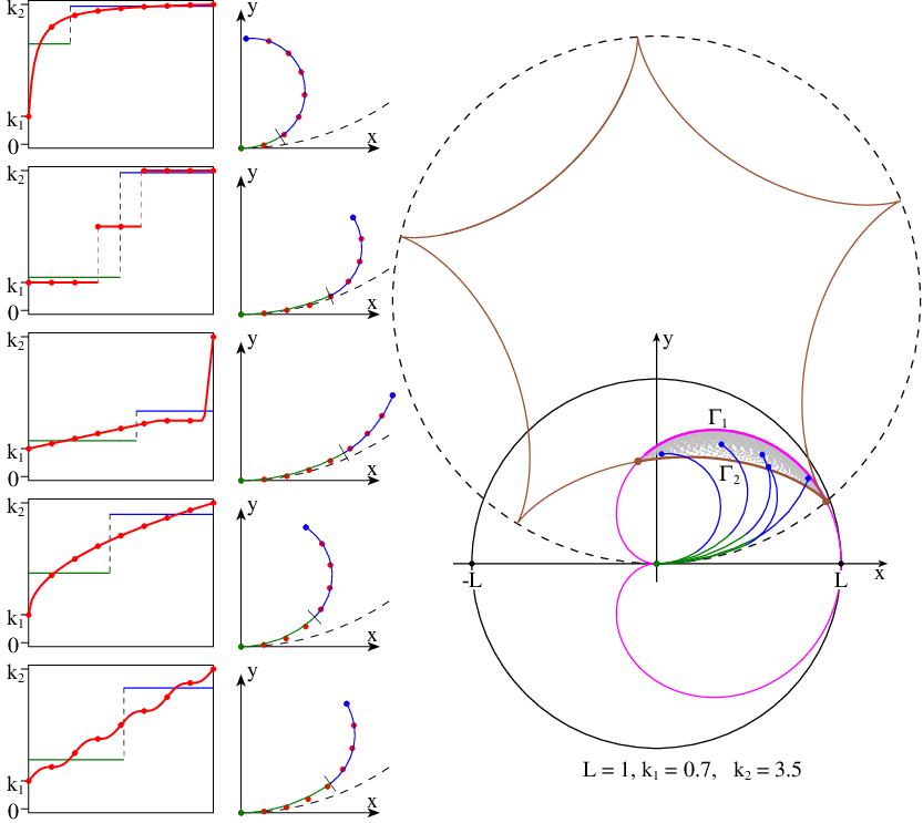
In [1] possible positions of the endpoint of a spiral arc with prescribed end curvatures k⁡(0)=k1k(0)=k_{1}, k⁡(L)=k2k(L)=k_{2}, and length LL are of interest. In Fig. 5 five examples of such arcs are traced. The left column shows plots of curvature k⁡(s)k(s), monotone increasing from k1k_{1} to k2k_{2}. There are also drawn two-level plots of curvatures k¯​(s)\bar{k}(s) of biarcs, approximating every spiral arc in terms of Theorem 1. Biarcs themselves are drawn in the second column, together with some points of the original (approximated) curve. Dashed arc is the circle of curvature {0,0,0,k1}\left\{0,0,0,k_{1}\right\} at the startpoint.

Refer to caption
Figure 5: Modelling of location of endpoints of a spiral arcs (case 0⩽k1<k20\leqslant k_{1}<k_{2})
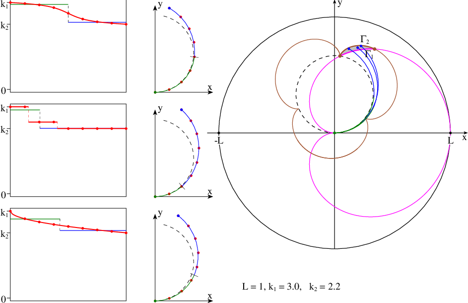
Refer to caption
Figure 6: Modelling of location of endpoints of a spiral arcs, the case k1>k2⩾0k_{1}>k_{2}\geqslant 0.

Let complex number Z1​(k,l)Z_{1}(k;l) denotes the endpoint of the circular arc, whose curvature and length are kk and ll, traced from the coordinate origin along the X-axis:

Z1(k;l)=∫0lei​k​sds=ik(1−ei​k​l)=2ksink​l2ei​k​l2[Z1(0;l)=limk→0Z1(k;l)=l].Z_{1}(k;l)=\displaystyle\int\limits_{0}^{l}{{\mathrm{e}}^{{\mathrm{i}}ks}}\,{\mathrm{d}}s=\frac{{\mathrm{i}}}{k}\left(1-{\mathrm{e}}^{{\mathrm{i}}kl}\right)=\frac{2}{k}\sin\frac{kl}{2}{\mathrm{e}}^{\frac{{\mathrm{i}}kl}{2}}\qquad\left[Z_{1}(0;l)=\lim\limits_{k\to 0}Z_{1}(k;l)=l\right].

Let Z2​(q1,l1,q2,l2)Z_{2}(q_{1},l_{1};q_{2},l_{2}) denotes the endpoint of the biarc, whose curvatures and lengths are q1,l1q_{1},l_{1}, and q2,l2q_{2},l_{2}:

Z2​(q1,l1,q2,l2)=Z1​(q1,l1)+ei​q1​l1​Z1​(q2,l2).Z_{2}(q_{1},l_{1};q_{2},l_{2})=Z_{1}(q_{1},l_{1})+{\mathrm{e}}^{{\mathrm{i}}q_{1}l_{1}}Z_{1}(q_{2},l_{2}).

For every curve in model (16) we calculate the endpoint as Z2​(q1,l1,q2,L−l1)Z_{2}(q_{1},l_{1};\,q_{2},L-l_{1}). The result of such procedure is shown in the right side of Fig. 5 as the pointset, bounded by curves Γ1\Gamma_{1} and Γ2\Gamma_{2}. As the hypotheses for bounds, the limitary cases of model (16) were thought of, namely:

  • •

    Vanishing of one of two arcs, i. e. either l1=0l_{1}=0, or l1=Ll_{1}=L: biarc (16) degenerates into the circular arc of curvature qq and length LL. With varying qq, the endpoints of these arcs trace parametric curve Γ1​(q)\Gamma_{1}(q) (17).

  • •

    Biarcs of the total length LL with curvatures, taking limit values q1=k1q_{1}=k_{1}, q2=k2q_{2}=k_{2}, the join point being varied. Their endpoints trace curve Γ2​(t)\Gamma_{2}(t):

    Γ1:x⁡(q)+i​y​(q)=Z1​(q,L),k1⩽q⩽k2;Γ2:x⁡(t)+i​y​(t)=Z2​(k1,L−t,k2,t),0⩽t⩽L.\begin{array}[]{lll}\Gamma_{1}{:}&x(q)+{\mathrm{i}}y(q)=Z_{1}(q;L),&k_{1}\leqslant q\leqslant k_{2};\\ \Gamma_{2}{:}&x(t)+{\mathrm{i}}y(t)=Z_{2}(k_{1},L{-}t;\,k_{2},t),&0\leqslant t\leqslant L.\end{array} (17)

In Fig. 5 curves Γ1,2\Gamma_{1,2} are extended beyond the parameter ranges, specified in (17). Curve Γ1\Gamma_{1} is known as cochleoid [8, p. 230]. Its polar equation is p⁡(φ)=L​sin⁡φφp(\varphi)=L\frac{\sin\varphi}{\varphi}.

Under conditions of Fig. 5 (0<k1<k20<k_{1}<k_{2}), curve Γ2\Gamma_{2} is hypocycloid. To bring it to the canonical position, one should move the coordinate origin to the point (0,k1−1)\left(0,k_{1}^{-1}\right), and apply rotation by the angle k1​L−π/2k_{1}L-{\pi}/2.

The output of modelling for the case of curvature, decreasing in the range k1>k2⩾0k_{1}>k_{2}\geqslant 0, is shown in Fig. 6 in the same manner. Bound Γ2\Gamma_{2} becomes epicycloid, or, if k2=0k_{2}=0, involute of initial circle of curvature.

Some more examples of such pointsets and their bounds are shown in Fig. 7. In the leftmost picture bound Γ2\Gamma_{2} becomes cycloid (k1=0k_{1}=0), or straight line segment (k2=2​k1k_{2}=2k_{1}). The last picture shows additionally subsets of endpoints, obtained by modelling with fixed value of turning angle

θ=∫0Lk⁡(s)​𝑑s=q1​l1+q2​(L−l1),\theta=\int_{0}^{L}k(s)ds=q_{1}l_{1}+q_{2}(L-l_{1}),

which is not affected by the approximation. Boundaries of these subsets are guessed as curves
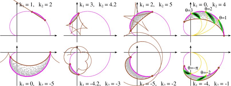
Z2​(q⁡(t),L−t,k2,t),\displaystyle Z_{2}(q(t),L{-}t;\,k_{2},t), where\displaystyle\text{where} q⁡(t)​(L−t)+k2​t=θ,\displaystyle q(t)(L-t)+k_{2}t=\theta, 0⩽\displaystyle 0\leqslant{} t⩽θ−k1​Lk2−k1,\displaystyle t\leqslant\frac{\theta-k_{1}L}{k_{2}-k_{1}},
and\displaystyle\text{and\penalty\ \penalty\ } Z2​(k1,L−t,q⁡(t),t),\displaystyle Z_{2}(k_{1},L{-}t;\,q(t),t), where\displaystyle\text{where} k1(L−t)+q(t)t=θ,\displaystyle k_{1}(L-t)+q(t)t=\theta,\quad θ−k1​Lk2−k1⩽\displaystyle\frac{\theta-k_{1}L}{k_{2}-k_{1}}\leqslant{} t⩽L.\displaystyle t\leqslant L.
Refer to caption
Figure 7: Other examples, with curvature decreasing, increasing, positive, negative.

4.2 Modelling of closeness of ovals

Oval is usually meant a closed convex curve. Additionally, we assume it to have the minimal number of verticez, i. e., exactly four, in virtue of the Four-vertex theorem. An example is given by curve V0​V1​V2​V3​V0V_{0}V_{1}V_{2}V_{3}V_{0} in Fig. 10a.

Consider the possibility of modelling curves with only one vertex, namely, with curvature k⁡(s)k(s), increasing from k⁡(0)=k1k(0)=k_{1} to k⁡(L1)=k2k(L_{1})=k_{2} on an arc of length L1L_{1}, and then decreasing to k⁡(L)=k3k(L)=k_{3} on an arc of length L2=L−L1L_{2}=L-L_{1}. We need an analogue of model (16), as before, piecewise constant, but with 2×3=62\times 3=6 free parameters. Fixation of total turning θ\theta of a curve decrements the number of degrees of freedom (and embedded loops) to five. An example of modelling of a set of endpoints for a curve with one vertex and fixed turning is shown in Fig. 10b.

As a candidate to oval, consider a curve with periodic curvature k⁡(s)⩾0k(s)\geqslant 0, having four extrema within the period s4=L1+L2+L3+L4s_{4}=L_{1}{+}L_{2}{+}L_{3}{+}L_{4}:

k1=k(0)=k(s4),k2=k(s1),k3=k(s2),k4=k(s3),andk1<k2>k3<k4>k1.k_{1}=k(0)=k(s_{4}),\quad k_{2}=k(s_{1}),\quad k_{3}=k(s_{2}),\quad k_{4}=k(s_{3}),\quad\text{and}\quad k_{1}<k_{2}>k_{3}<k_{4}>k_{1}.

Several versions of k⁡(s)k(s) with prescribed si,kis_{i},k_{i} are shown below:

[Uncaptioned image] (18)

Denote curves, generated by such curvature function, as V0​V1​V2​V3​V4V_{0}V_{1}V_{2}V_{3}V_{4}. The curve is oval if:

(a) ​∫0s4k⁡(s)​𝑑s=2​π;(b) ​V0=V4.\text{(a)\penalty\ }\textstyle\int\limits_{0}^{s_{4}}{k(s)}\mathrm{d}s=2\pi;\quad\text{(b)\penalty\ }V_{0}=V_{4}.

Let μ=∫0s2k⁡(s)​𝑑s\mu=\int\limits_{0}^{s_{2}}{k(s)}\mathrm{d}s and ν=∫s1s3k⁡(s)​𝑑s\nu=\int\limits_{s_{1}}^{s_{3}}{k(s)}\mathrm{d}s be the turning angles between two opposite verticez, those of minimal curvature (μ\mu, arc V0​V1​V2V_{0}V_{1}V_{2}), and those of maximal curvature (ν\nu, arc V1​V2​V3V_{1}V_{2}V_{3}). For μ\mu, and for turning 2​π−μ2\pi-\mu on the complementary arc V2​V3​V0V_{2}V_{3}V_{0} we have natural restrictions (here L1=s1L_{1}=s_{1}, L2=s2−s1L_{2}=s_{2}-s_{1}, L3=s3−s2L_{3}=s_{3}-s_{2}, L4=s4−s3L_{4}=s_{4}-s_{3}):

k1L1+k3L2<μ<k2(L1+L2),k3L3+k1L4<2π−μ<k4(L3+L4)⟹k_{1}L_{1}+k_{3}L_{2}<\mu<k_{2}(L_{1}+L_{2}),\quad k_{3}L_{3}+k_{1}L_{4}<2\pi-\mu<k_{4}(L_{3}+L_{4})\quad\Longrightarrow\quad
max⁡(k1​L1+k3​L2, 2​π−k4​(L3+L4))<μ<min⁡(k2​(L1+L2), 2​π−(k3​L3+k1​L4)).\max\left(k_{1}L_{1}+k_{3}L_{2},\,2\pi-k_{4}(L_{3}+L_{4})\right)<\mu<\min\left(k_{2}(L_{1}+L_{2}),\,2\pi-(k_{3}L_{3}+k_{1}L_{4})\right). (19)

Restrictions for ν\nu can be derived similarly.

Refer to caption
Figure 8: Oval V0​V1​V2​V3​V0V_{0}V_{1}V_{2}V_{3}V_{0}, and modelling of possible locations of vertex V2V_{2}


Refer to caption

Figure 9: Testing closeness of ovals (20). Sets of endpoints (with one example of generating curve for each set), obtained by varying parameter μ\mu.


Refer to caption

Figure 10: In (20) the value k1=0.25k_{1}=0.25 is replaced by k1=0.42k_{1}=0.42; sets do not intersect.

Let us subdivide oval V0​V1​V2​V3​V0V_{0}V_{1}V_{2}V_{3}V_{0} into two curves, each with one vertex.

  • •

    The first curve, V0​V1​V2V_{0}V_{1}V_{2}, is traced from the coordinate origin along the direction 𝐧⁡(−π2)\mathbf{n}\left(-\frac{\pi}{2}\right). Its turning μ\mu is fixed, the set A1​B1​C1​D1​A1A_{1}B_{1}C_{1}D_{1}A_{1} of possible endpoints V2V_{2} is shown in Fig. 10b.

  • •

    The second curve, V0​V3​V2V_{0}V_{3}V_{2}, is obtained by reversing the curve V2​V3​V0V_{2}V_{3}V_{0}. Its curvature function is k~​(s)=−k⁡(s4−s)\widetilde{k}(s)=-k(s_{4}{-}s), 0⩽s⩽s4−s20\leqslant s\leqslant s_{4}{-}s_{2}. The curve starts from the coordinate origin along the direction 𝐧⁡(π2)\mathbf{n}\left(\frac{\pi}{2}\right). Its turning angle μ−2​π\mu-2\pi is fixed such as to get smooth closeness, if endpoints of the two curves come to coincidence. The set A2​B2​C2​D2​A2A_{2}B_{2}C_{2}D_{2}A_{2} of possible endpoints V2V_{2} of the second curve is shown in Fig. 10c.

Non-empty intersection of two sets (Fig. 10d) means that, with given μ\mu, a common point V2V_{2} exists, and constructing closed curve V0​V1​V2​V3​V0V_{0}V_{1}V_{2}V_{3}V_{0} is possible. Empty intersection would signify that with given μ\mu closeness is impossible. Fig. 10 with

k1=0.25,L1=3.5,k2=0.80,L2=3.2,k3=0.07,L3=4.3,k4=0.85,L4=4.0,k_{1}=0.25,\;L_{1}=3.5,\quad k_{2}=0.80,\;L_{2}=3.2,\quad k_{3}=0.07,\;L_{3}=4.3,\quad k_{4}=0.85,\;L_{4}=4.0, (20)

shows how the mutual position of two sets changes as μ\mu varies. One of sets vanishes as μ\mu reaches limits (19). Two sets approach each other as μ\mu increases from minimum, come to contact at μ≈0.79​π\mu\approx 0.79\pi, intersect each other, and diverge after μ≈1.07​π\mu\approx 1.07\pi.

A lot of tests discovered two kinds of behavior:

  1. 1.

    The sets approach each other, intersect between two contact positions, and separate thereafter. Tangency of curves A​BAB and C​DCD, demonstrated in Fig. 10, is not the only way of contact.

  2. 2.

    Two sets pass around each other, without coming to contact (Fig. 10).

Similar behavior was observed when parameter ν\nu was varied. These observations lead to the following hypotheses about closeness of ovals.

  1. 1.

    Closeness requires restrictions μ′<μ<μ′′\mu^{\prime}<\mu<\mu^{\prime\prime}, ν′<ν<ν′′\nu^{\prime}<\nu<\nu^{\prime\prime}, essentially more narrow than natural restrictions (19). The values of μ′,μ′′,ν′,ν′′\mu^{\prime},\mu^{\prime\prime},\nu^{\prime},\nu^{\prime\prime} are solutions of some equations Fj​(x,Li,ki)=0F_{j}(x;L_{i},k_{i})=0, describing contact of boundary curves.

  2. 2.

    The values Li,kiL_{i},k_{i} exist, such that closeness of curve (18) is impossible for whatever profile k⁡(s)k(s). We cannot specify whether this fact is reflected as μ′′⩽μ′\mu^{\prime\prime}\leqslant\mu^{\prime} (ν′′⩽ν′\nu^{\prime\prime}\leqslant\nu^{\prime}), or as the absence of solutions of the above mentioned equations.

  3. 3.

    These restrictions are necessary for closeness of the curve, and sufficient for existence of an oval with given parameters Li,kiL_{i},k_{i}, i=1,2,3,4i=1,2,3,4.

With rather simple and clear graphic representation, we come across bulky formulas, which seems inevitable, as soon as high order cycloidal curves become involved. E. g., bound A1​B1​(u)A_{1}B_{1}(u) is

e−i​π2⋅Z2​(q1​(u),L1,q2​(u),L2),q1​(u)=μ−2​u​L2L1+L2,q2​(u)=μ+2​u​L1L1+L2,{k1⩽q1​(u)⩽k2,k2⩾q2​(u)⩾k3{\mathrm{e}}^{-{\mathrm{i}}\frac{\pi}{2}}\cdot Z_{2}(q_{1}(u),L_{1};\,q_{2}(u),L_{2}),\quad q_{1}(u)=\frac{\mu-2uL_{2}}{L_{1}+L_{2}},\quad q_{2}(u)=\frac{\mu+2uL_{1}}{L_{1}+L_{2}},\quad\begin{cases}k_{1}\leqslant q_{1}(u)\leqslant k_{2},\\ k_{2}\geqslant q_{2}(u)\geqslant k_{3}\end{cases}

(q1​L1+q2​L2=μq_{1}L_{1}+q_{2}L_{2}=\mu). Bound C1​D1​(v)C_{1}D_{1}(v) is e−i​π2​Z3​(k1,l1​(v),k2,l2​(v),k3,l3​(v)){\mathrm{e}}^{-{\mathrm{i}}\frac{\pi}{2}}Z_{3}(k_{1},l_{1}(v);\,k_{2},l_{2}(v);\,k_{3},l_{3}(v)), with Z3Z_{3} defined as

Z3​(q1,l1,q2,l2,q3,l3)=Z1​(q1,l1)+ei​q1​l1​Z1​(q2,l2)+ei⁡(q1​l1+q2​l2)​Z1​(q3,l3),Z_{3}(q_{1},l_{1};\,q_{2},l_{2};\,q_{3},l_{3})=Z_{1}(q_{1},l_{1})+{\mathrm{e}}^{{\mathrm{i}}q_{1}l_{1}}Z_{1}(q_{2},l_{2})+{\mathrm{e}}^{{\mathrm{i}}(q_{1}l_{1}+q_{2}l_{2})}Z_{1}(q_{3},l_{3}),

with l1,2,3​(v)l_{1,2,3}(v) and the range for vv defined from

{l1​(v)+l2​(v)+l3​(v)=L1+L2,k1​l1​(v)+k2​l2​(v)+k3​l3​(v)=μ,l3​(v)−l1​(v)=2​v;{0⩽l1​(v)⩽L1,0⩽l3​(v)⩽L2.\begin{cases}l_{1}(v)+l_{2}(v)+l_{3}(v)=L_{1}+L_{2},\\ k_{1}l_{1}(v)+k_{2}l_{2}(v)+k_{3}l_{3}(v)=\mu,\\ l_{3}(v)-l_{1}(v)=2v;\end{cases}\qquad\begin{cases}0\leqslant l_{1}(v)\leqslant L_{1},\\ 0\leqslant l_{3}(v)\leqslant L_{2}.\end{cases}

We also note that these hypotheses got a concrete form in the particular case

L1=L2=L3=L4=L,k1=k3⩾0,k2=k4>k1.L_{1}=L_{2}=L_{3}=L_{4}=L,\qquad k_{1}=k_{3}\geqslant 0,\qquad k_{2}=k_{4}>k_{1}.

Namely, denote

ϰ1=k1​L,ϰ2=k2​L,Φ⁡(x,p,q)=q⁡(x+2​p)​sin⁡x2−x⁡(q−p)​sin⁡q⁡(2​p+x−2​π)2​(q−p).\varkappa_{1}=k_{1}L,\quad\varkappa_{2}=k_{2}L,\qquad\Phi(x;p,q)=q(x+2p)\sin\frac{x}{2}-x(q-p)\sin\frac{q(2p+x-2\pi)}{2(q-p)}.

The necessary condition of smooth closeness, ∫04​Lk⁡(s)​𝑑s=2​π\int\limits_{0}^{4L}k(s)\,\mathrm{d}s=2\pi, requires for an oval

k1​(L1+L4)+k3​(L2+L3)<2​π<k2​(L1+L2)+k4​(L3+L4)⟹0⩽ϰ1<π2<ϰ2,k_{1}(L_{1}+L_{4})+k_{3}(L_{2}+L_{3})<2\pi<k_{2}(L_{1}+L_{2})+k_{4}(L_{3}+L_{4})\quad\Longrightarrow\quad 0\leqslant\varkappa_{1}<\frac{\pi}{2}<\varkappa_{2},

and (19) looks like

if ​ϰ1+ϰ2⩽π:\displaystyle\text{if\penalty\ \penalty\ }\varkappa_{1}+\varkappa_{2}\leqslant\pi{:} 2​π−2​ϰ2<\displaystyle 2\pi-2\varkappa_{2}<{} μ<2​ϰ2,\displaystyle\mu<2\varkappa_{2}, (21)
if ​ϰ1+ϰ2⩾π:\displaystyle\text{if\penalty\ \penalty\ }\varkappa_{1}+\varkappa_{2}\geqslant\pi{:} 2​ϰ1<\displaystyle 2\varkappa_{1}<{} μ<2​π−2​ϰ1\displaystyle\mu<2\pi-2\varkappa_{1}

(ν\nu is in the same range). We observe in this case the following.

  1. 1.

    Intersection of two sets always occurs, starting with tangency of bounds A2​B2A_{2}B_{2} and C1​D1C_{1}D_{1} at μ=μ′\mu=\mu^{\prime}, ending with tangency of A1​B1A_{1}B_{1} and C2​D2C_{2}D_{2} at μ=μ′′\mu=\mu^{\prime\prime} (and likewise in modelling for ν\nu). Under the above parametrizations, A1​B1​(u)A_{1}B_{1}(u), C1​D1​(v)C_{1}D_{1}(v), and similar ones for A2​B2​(u)A_{2}B_{2}(u), C2​D2​(v)C_{2}D_{2}(v), tangencies occur at u=0u=0 and v=0v=0.

  2. 2.

    Equations for μ′,μ′′,ν′,ν′′\mu^{\prime},\mu^{\prime\prime},\nu^{\prime},\nu^{\prime\prime} are:

    Φ⁡(μ′′,ϰ1,ϰ2)=0,Φ⁡(ν′,ϰ2,ϰ1)=0,μ′=2​π−μ′′,ν′′=2​π−ν′.\Phi(\mu^{\prime\prime};\varkappa_{1},\varkappa_{2})=0,\quad\Phi(\nu^{\prime};\varkappa_{2},\varkappa_{1})=0,\quad\mu^{\prime}=2\pi-\mu^{\prime\prime},\quad\nu^{\prime\prime}=2\pi-\nu^{\prime}.

    Numerical verification shows existence and uniqueness of solutions in ranges (21).

5 Further work

In conclusion, we announce some results, already studied by the author, and concerning the further development of the subject.

Using approximation with spiral triarcs (instead of biarcs) reproduces, together with boundary tangents, also boundary curvatures, i. e. the two-point G2 Hermite data of the original curve. Approximation problem with length preservation always has one or two solutions; the second one appears for arcs with inflection.

If the curve, split into nn spiral arcs, is approximated by triarcs, we get 3​n3n circular arcs instead of 2​n2n, given by biarcs method. But, for every inner node, the curvature of the left-sided arc is equal to that of the right-sided arc, both being equal to the curvature k⁡(si)k(s_{i}) of the original curve in the node. These two arcs can be merged, and the approximating curve will be composed of 2​n+12n+1 arcs (or still of 2​n2n, if the original curve was closed).

For approximation with triarcs, two-level model (16) is replaced by three-level one:

[Uncaptioned image]

The family of approximating curves remains three-parametric, so, implementation of modelling procedure requires the same depth of embedded loops as in the biarcs case.

Using triarcs approximation does not require convexity of the original arc. Therefore, there is no need to include inflection points into initial splitting of a curve. Taking into account applications to conformal maps, mentioned in [1], this feature resonates with the fact that, e. g., under Möbius map of both the curve and its approximation, verticez remain such [4, Cor. 1.1]. Inflection points are not thus invariant: they can shift along the mapped curve, appear on, or disappear from it.

References

  • [1] Sabitov I. Kh., Slovesnov A. V. Approximation of plane curves by circular arcs. Computational Math. and Math. Physics, 2010, Vol. 50, No. 8, pp. 1279–1288.
  • [2] Kurnosenko A.I. General properties of spiral plane curves. Journal of Math. Sciences, 161, No. 3(2009), 405-418. (transl. from Zapiski nauch. sem. POMI, 353(2008), 93–115).
  • [3] Bolton K.M. Biarc curves. Comp.-Aided Design, 7(1975), N 2, 89–92.
  • [4] Kurnosenko A.I. An inversion invariant of a pair of circles. Journal of Math. Sciences, 110, No. 4(2002), 2848–2860. (translated from Zapiski nauch. sem. POMI, 261(1999), 167–186).
  • [5] Kurnosenko A.I. Short spirals. Journal of Math. Sciences, 175, No. 5(2011), 517-522. (transl. from Zapiski nauch. sem. POMI, 372(2009), 34–43).
  • [6] Kurnosenko A.I. Biarcs and bilens. Comp. Aided Geom. Design, 30 (2013), 310–330.
  • [7] Alexandrov A. D. Intrinsic Geometry of Convex Surfaces. CRC, Boca Raton, 2006, p. 411 (OGIZ, Moscow, 1948; p. 373).
  • [8] Savelov A.A. Planar curves. Systematics, properties, applications. Moscow, Fizmatgiz, 1960.