msam10 \correspondChristiane Notarmarco, Springer-Verlag London Limited, Sweetapple House, Catteshall Road, Godalming, Surrey GU7 3DJ, UK. e-mail: chris@svl.co.uk \pagerangeModeling and Efficient Verification of Wireless Ad hoc Networks–References
Modeling and Efficient Verification of Wireless Ad hoc Networks
Abstract
Wireless ad hoc networks, in particular mobile ad hoc networks (MANETs), are growing very fast as they make communication easier and more available. However, their protocols tend to be difficult to design due to topology dependent behavior of wireless communication, and their distributed and adaptive operations to topology dynamism. Therefore, it is desirable to have them modeled and verified using formal methods. In this paper, we present an actor-based modeling language with the aim to model MANETs. We address main challenges of modeling wireless ad hoc networks such as local broadcast, underlying topology, and its changes, and discuss how they can be efficiently modeled at the semantic level to make their verification amenable. The new framework abstracts the data link layer services by providing asynchronous (local) broadcast and unicast communication, while message delivery is in order and is guaranteed for connected receivers. We illustrate the applicability of our framework through two routing protocols, namely flooding and AODVv2-11, and show how efficiently their state spaces can be reduced by the proposed techniques. Furthermore, we demonstrate a loop formation scenario in AODV, found by our analysis tool.
keywords
state-space reduction; mobile ad hoc network; ad hoc routing protocol; Rebeca; actor-based language; model checking.1 Introduction
Applicability of wireless communications is rapidly growing from home networks to satellite transmissions due to their high accessibility and low cost. Wireless communication has a broadcasting nature, as messages sent by each node can be received by all nodes in its transmission range, called local broadcast. Therefore, by paying the cost of one transmission, several nodes may receive the message, which leads to lower energy consumption for the sender and throughput improvement [CCH07].
Mobile ad hoc networks (MANETs) consist of several portable hosts with no pre-existing infrastructure, such as routers in wired networks or access points in managed (infrastructure) wireless networks. In such networks, nodes can freely change their locations so the network topology is constantly changing. For unicasting a message to a specific node beyond the transmission range of a node, it is needed to relay the message by some intermediate nodes to reach the desired destination. Due to lack of any pre-designed infrastructure and global network topology information, network functions such as routing protocols are devised in a completely distributed manner and adaptive to topology changes. Topology dependent behavior of wireless communication, distribution and adaptation requirements make the design of MANET protocols complicated and more in need of modeling and verification so that it can be trusted. For instance, MANET protocols like the Ad hoc On Demand Distance Vector (AODV) routing protocol [PB99] has been evolved as new failure scenarios were experienced or errors were found in the protocol design [BOG02, NT15b, FVGH+13].
The actor model [Agh90, Hew77] has been introduced for the purpose of modeling concurrent and distributed applications. It is an agent-based language introduced by Hewitt [Hew77], extended by Agha to an object-based concurrent computation model [Agh90]. An actor model consists of a set of actors communicating with each other through unicasting asynchronous messages. Each computation unit, modeled by an actor, has a unique address and mailbox. Messages sent to an actor are stored in its mailbox. Each actor is defined through a set of message handlers, called message servers, to specify the actor behavior upon processing of each message. In this model, message delivery is guaranteed but is not in-order. This policy implicitly abstracts away from effects of the network, i.e., delays over different routing paths, message conflicts, etc., and consequently makes it a suitable modeling framework for concurrent and distributed applications. Rebeca [SMSdB04] is an actor-based modeling language which aims to bridge the gap between formal verification techniques and the real-world software engineering of concurrent and distributed applications. It provides an operational interpretation of the actor model through a Java-like syntax, which makes it easy to learn and use. Rebeca is supported by a robust model checking tool, named Afra [afrb], which takes advantage of various reduction techniques [JSM+10, SS10] to make efficient verification possible. With the aim of reducing the state space, computations, i.e., executions of message servers in actors, are assumed to be instantaneous while message delivery is in-order. Consequently, instructions of message servers are not interleaved and hence, execution of message servers becomes atomic in semantic model and each actor mailbox is modeled through a FIFO queue.
In [YGK15] we introduced bRebeca as an extension to Rebeca, to support broadcast communication which abstracts the global broadcast communications [BG92]. To abstract the effect of network, the order of receipts for two consequent broadcast communications is not necessarily the same as their corresponding sends in an actor model. Hence, each actor mailbox was modeled by a bag. The resulting framework is suitable for modeling and efficient verification of broadcasting protocols above the network layer, but not appropriate for modeling MANETs in two ways: firstly the topology is not defined, and every actor (node) can receive all messages, in other words all nodes are connected to each other. Secondly, as there is no topology defined, mobility is not concerned.
In this paper, we extend the actor-based modeling language bRebeca [YGK15] to address local broadcast, topology, and its changes. The aim of the current paper is to provide a framework to detect malfunctions of a MANET protocol caused by conceptual mistakes in the protocol design, rather than by an unreliable communication. Therefore, the new framework abstracts away from the data link layer services by providing asynchronous reliable local broadcast, multicast, and unicast communications [Pen08, SL04]. Since only one-hop communications are considered, the message delivery is in-order and is guaranteed for connected receivers. Consequently, each actor mailbox is modeled through a queue. The reliable communication services of the data link layer provide feedback (to its upper layer applications) in case of (un)successful delivery. Therefore, our framework provides conditional unicast to model protocol behaviors in each scenario (in the semantic model, the status of the underlying topology defines the behavior of actors).
The resulting framework provides a suitable means to model the behavior of ad hoc networks in a compositional way without the need to consider asynchronous communications handled by message storages in the computation model. However, to minimize the effect of message storages on the growth of the state space, we exploit techniques to reduce it. Since nodes can communicate through broadcast and a limited form of multicast/unicast, it is possible to consider actors that have the same neighbors and local states as identical according to the counter abstraction technique [BMWK09, PXZ02, ET99]. Therefore, the states whose number of actors (irrespective of their identifiers) with the same neighbors and local state are the same for each local state value, will be aggregated, thus the state space is reduced considerably. The reduced semantics is strongly bisimilar to the original one.
To examine resistance and adaptation of MANET protocols to changes of the underlying topology, we address mobility via arbitrary changes of the topology at the semantic level. Since network protocols have no control over movement of MANET nodes and mobility is an intrinsic characteristic of such nodes, the topology should be implicitly manipulated at the semantics. In other words, with the aim of verifying behaviors of MANET protocols for any mobility scenario, the underlying topology is arbitrarily changed at each semantic state. We provide mechanisms to restrict this random changes in the topology through specifying constraints over the topology. However, these random changes make the state space grow exponentially while the proposed counter abstraction technique becomes invalid. To this end, each state is instead explored for each possible topology and meanwhile topology information is removed from the state. Therefore, two next states only different in their topologies are consolidated together and hence, the state space is reduced considerably. Due to arbitrary changes of the underlying topology, states with different topologies are reachable from each other (through -transitions denoting topology changes). We establish that such states are branching bisimilar, and consequently a set of properties such as ACTL-X [DV90] are preserved. The proposed reduction techniques makes our framework scalable to verify some important properties of MANET protocol, e.g., loop freedom, in the presence of mobility in a unified model (cf. generating a model for each mobility scenario).
The contributions of this paper can be summarized as follows:
- •
We extend the computation model of the actor model, in particular Rebeca, with the concepts of MANETs, i.e., asynchronous reliable local broadcast/multicast/unicast, topology, and topology changes;
- •
We apply the counter abstraction in presence of topology as a part of semantic states to reduce state space substantially: actors with the same neighbors, i.e., topological situations, and local states are counted together in the counter abstraction technique;
- •
We show that the soundness of the counter abstraction technique is not preserved in presence of mobility, and propose another technique to reduce the state space.
- •
We provide a tool that supports both reduction techniques and examines invariant properties automatically. We illustrate the scalability of our approach through the specification and verification of two MANET protocols, namely flooding and AODV.
- •
We present a complete and accurate model of the core functionalities of a recent version of AODVv2 protocol (version 11), abstracting from its timing issues, and investigate its loop freedom property. We detect scenarios over which the property is violated due to maintaining multiple unconfirmed next hops for a route without checking them to be loop free. We have communicated this scenario to the AODV group and they have confirmed that it can occur in practice. In response, their route information evaluation was modified, published in version of the draft.11 1 https://tools.ietf.org/html/draft-ietf-manet-aodvv2-13 Furthermore, we verify the monotonic increase of sequence numbers and packet delivery properties using existing model checkers.
Our framework can also be applied to Wireless Mesh Networks (WMNs). Unlike MANETs, WSNs have a backbone of dedicated mesh routers along with mesh clients. Hence, they provide flexibility in terms of mobility: in contrast to MANETs, the clients mobility has limited effect on the overall network configuration, as the mesh routers are fixed [MKKAR06].
The paper is structured as follows. Section 2 briefly introduces bRebeca, explain the idea behind the counter abstraction technique and its relation to symmetry reduction technique, and explains equivalence relations that validate our reduction techniques. Section 3 addresses the main modeling challenges of wireless networks. Section 4 presents our extension to bRebeca for modeling MANETs. In Section 5, we generate the state space compactly with the aim of efficient model checking. To illustrate the applicability of our approach, we specify the core functionalities of AODVv2-11 in Section 6. Then, in Section 7, we discuss the efficiency of our state-space generation over two cases studies: the AODV and the flooding-based routing protocol. We illustrate our tool and possible analysis over the models through a verification of AODV. Finally, we review some related work in Section 8 before concluding the paper.
2 Preliminaries
2.1 bRebeca
Rebeca [SMSdB04] is an actor-based modeling language proposed for modeling and verification of concurrent and distributed systems. It has a Java-like syntax familiar to software developers and it is also supported by a tool via an integrated modeling and verification environment [afrb]. Due to its design principle it is possible to extend the core language based on the desired domain [SJ11]. For example, different extensions have been introduced in various domains such as probabilistic systems [VK12], real-time systems [RSA+14], software product lines [SK13], and broadcasting environment [YGK15]. As in this paper we intend to extend bRebeca, we briefly review its syntax and semantics.
In bRebeca as well as in Rebeca, actors are the computation units of the system, called rebecs (short for reactive objects), which are instances of the defined reactive classes in the model.
Rebecs communicate with each other only through broadcasting message which is asynchronous. Every sent message eventually will be received and processed by its potential receivers. In Rebeca, the rebecs defined as the known rebecs of a sender, the sender itself using the “self” keyword, or the sender of the message currently processed using the keyword “sender” are considered as the potential receivers. However, in bRebeca, it is assumed the network is fully connected and therefore, all rebecs of a model constitute the potential receivers. In other words, a broadcast message is received by all the nodes to which a sender has a (one-hop/multi-hop) path. So, unlike Rebeca, there is no need for declaring the known rebecs in the reactive class definition. Due to unpredictability of multi-hop communications, the arrival order of messages must be considered arbitrary. Therefore, as the second difference with Rebeca, received messages are stored in an unordered bag in each node.
Every reactive class has two major parts, first the state variables to maintain the state of the rebec, and second the message servers to indicate the reactions of the rebec on received messages. The local state of a rebec is defined in terms of its state variables together with its message bag. Whenever a rebec receives a message which has no corresponding message server to respond to, it simply discards the message. Each rebec has at least one message server called “initial”, which acts like a constructor in object-oriented languages and performs the initialization tasks.
A rebec is said to be enabled if and only if it has at least one message in its bag. The computation takes place by removing a message from the bag and executing its corresponding message server atomically, after which the rebec proceeds to process the other messages in its bag (if any). Processing a message may have the following consequences:
- •
it may modify the value of the state variables of the executing rebec, or
- •
some messages may be broadcast to other rebecs.
Each bRebeca model consists of two parts, the reactive classes part and the main part. In the main part the instances of the reactive classes are created initially while their local variables are initialized.
As an example, Figure 1 illustrates a simple max finding algorithm modeled in bRebeca, referred to as “Max-Algorithm” [DK86]. Every node in a network contains an integer value and they intend to find the maximum value of all nodes in a distributed manner. The initial message server has a parameter, named starter. The rebec with the starter value initiates the algorithm by broadcasting the first message. Whenever a node receives a value from others, it compares this value with its current value and one of the following scenarios happens:
- •
if it has not broadcast its value yet and its value is greater than the received one, it broadcasts its value to others;
- •
if its current value is less than the received one, it gives up broadcasting its value and updates its current value to the received one;
- •
if it has already sent its value, it only checks whether it must updates its value.
This protocol does not work on MANETs as nodes give up to rebroadcast their value after their first broadcast. The Max-Algorithm should find the maximum value among the connected nodes in MANETs. To this aim, if a node moves and connects to new nodes, it has to re-send its value as its value may be the maximum value in the currently connected nodes.
2.2 Counter Abstraction
Since model checking is the main approach of verification in Rebeca, we need to overcome state-space explosion, where the state space of a system grows exponentially as the number of components in the system increases. One way to tackle this well-known problem is through applying reduction techniques such as symmetry reduction [CEJS98] and counter abstraction [BMWK09, PXZ02, ET99]. Counter abstraction is indeed a form of symmetry reduction and, in case of full symmetry, it can be used to avoid the constructive orbit problem, according to which finding a unique representative of each state is NP-hard [CEJS98]. The idea of using counters and counter abstraction in model checking was first introduced in [ET99]. However, the term of counter abstraction was first presented in [PXZ02] for the verification of parameterized systems and further used in different studies such as [BMWK09, Kat11].
The idea of counter abstraction is to record the global state of a system as a vector of counters, one per local state. Each counter denotes the number of components currently residing in the corresponding local state. In our work, by“components” we mean the actors of the system. This technique turns a model with an exponential size in , i.e. , into one of a size polynomial in , i.e. , where and denote the number of components and local states, respectively. Two global states and are considered identical up to permutation if for every local state , the number of components residing in is the same in the two states and , as permutation only changes the order of elements. For example, consider a system which consists of three components that each have only one variable of boolean type. Three global states , , and are equivalent and can be abstracted into one global state represented as .
2.3 Semantic Equivalence
Strong bisimilarity [Plo81] is used as a verification tool to validate the counting abstraction reduction technique on labeled transition systems. A labeled transition system (LTS), is defined by the quadruple where is a set of states, a set of transitions, a set of labels, and the initial state. Let denote .
Definition 2.1 (Strong Bisimilarity)
A binary relation is called a strong bisimilation if and only if, for any , and and , the following transfer conditions hold:
- •
,
- •
.
Two states and are called strong bisimilar, denoted by , if and only if there exists a strong bisimulation relating and .
As explained in Section 1, mobility is addressed through random changes of underlying topology at each semantic state, modeled by -transitions. We propose to remove such transitions while the behavior of each semantic state is explored for all possible topologies. We exploit branching bisimilarity [vGW96] to establish the reduced semantic is branching bisimilar to the original one. Let be reflexive and transitive closure of -transitions:
- •
;
- •
, and , then .
Definition 2.2 (Branching Bisimilarity)
A binary relation is called a branching bisimilation if and only if, for any , and and , the following transfer conditions hold:
- •
,
- •
.
Two states and are called branching bisimilar, denoted by , if and only if there exists a branching bisimulation relating and .
3 Modeling Topology and Mobility
In this section, we discuss issues brought up by extending bRebeca to model and verify MANETs, and our solutions to overcome these challenges. We assume that the number of nodes is fixed (to make the state space finite as explained in [DSZ11]).
3.1 Network Topology and Mobility
Every rebec represents a node in the MANET model. A node can communicate only with those located in its communication range, so-called connected. bRebeca does not define a “topology” concept as the network graph is considered to be connected, all nodes are globally connected.
Mobility is the intrinsic characteristic of MANET nodes. Furthermore, network protocols have no control over the movement of MANET nodes, and hence, topology changes cannot be specified as a part of the specification. Additionally, to verify a protocol with respect to any mobility scenario, we need to consider all possible topology changes while constructing the state space. To this end, we consider the topology as a part of the states and randomly change the underlying topology at the semantic level. To this aim, a topology is modeled as an matrix in each (global) state of the semantic model, where is the number of nodes in the network. Each element of this matrix, denoted by , indicates whether is connected to () or not (). As the communication ranges of all nodes are assumed to be equal, connectivity is a bidirectional concept, and hence, the resulting matrix will be symmetric. The main diagonal elements are always to make it possible for nodes to unicast messages to themselves. (However, in the case of broadcast, our semantic rules prevent a node from receiving its own message, see Section 4.2). Changing the topology is considered an unobservable action, modeled by a transition, which alters the topology matrix. Hence, each -transition represents a set of (bidirectional) link setups/breakdowns in the underlying topology.
To set up the initial topology of the network, the known-rebecs definitions, provided by the Rebeca language, is extended to address the connectivity of rebecs. Figure 2(a) shows the communication range of the nodes in a simple network. To configure the initial topology of this network, known-rebecs of each rebec should be defined as shown in Figure 2(b) during its instantiation (cf. Figure 1). The corresponding semantic representation (as a part of the initial state) is shown in Figure 2(c).
The connectivity matrix has elements which can be either or , and since on the main diagonal we will exclusively have s, we have possible topologies. For example, in a network of nodes, we have possible topologies. Considering all these topologies may lead to a state-space explosion. Hence, we provide a mechanism to limit the possible topologies by applying some network constraints to characterize the set of topologies in terms of (dis)connectivity relations to (un)pin a set of the links among the nodes. We use the notations or to show that two nodes and are connected or disconnected, respectively, and to denote both and hold. For example, specifies that () never gets connected to (), in other words, never enters into ’s communication range, and vice versa. Therefore a topology is called valid for the network constraint , denoted as , if:
where represents the element of the corresponding semantic model of , and characterizes all possible topologies.
If the only valid topology of a network constraint is equal to the initial topology, then the underlying topology will be static. This case can be useful for modeling WMNs with stable mesh routers with no mesh clients.
3.2 Restricted Delivery Guarantee
The nature of communications in the wireless networks is based on broadcast. The aim of the current paper is to provide a framework to detect malfunctions of a MANET protocol caused by conceptual mistakes in the protocol design, rather than by an unreliable communication. Therefore, we consider the wireless communications in our framework, namely local broadcast, multicast, and unicast, to be asynchronous and reliable in order to abstract the data link layer services. In this way, we abstract the issues related to contention management and collision detection following the approach of [KLN11]. This work abstracts the services of data link layer22 2 Data link layer (the second layer of Open Systems Interconnection (OSI) model) is responsible for transferring data across the physical link. It consists of two sublayers: Logical Link Control sublayer (LLC) and Media Access Control sublayer (MAC). LLC is mainly responsible for multiplexing packets to their protocol stacks identified by their IP addresses, while MAC manages accesses to the shared media. with the aim to design/analyze MANET protocols irrespective to the network radio model that implements them (its effect is captured by three delays functions). It provides reliable local broadcast communication, with timing guarantees on the worst-case amount of time for a message to be delivered to all its recipients, total amount of time the sender receives its acknowledgment, and the amount of time for a receiver to receive some message among those currently being transmitted by its neighbors, expressed by delay functions. Therefore, our approach to specify protocols relying on the abstract data link layer simplifies the study of such protocols, and is valid as its real implementation with such reliable services exists [Pen08, SL04]. In these implementations, a node can broadcast/multicast/unicast a message successfully only to the nodes within its communication range. Therefore, message delivery is guaranteed for the connected nodes to the sender. In the case of unicast, if the sender is located in the receiver communication range, it will be notified, otherwise it assumes that the transmission was unsuccessful so it can react appropriately. Therefore, we extended bRebeca with conditional unicast so that it enables the model to react accordingly based on the status of underlying topology (which defines the delivery status in reliable communications).
Since we only consider one-hop communications (in contrast to the broadcast in bRebeca), the assumption about the unpredictability of multi-hop communications (with different delays) is not valid anymore, and message storages in wRebeca are modeled by queues instead of bags.
4 wRebeca: Syntax and Semantics
In this section, we extend the syntax of bRebeca, introduced in Section 2.1, with conditional unicast and multicast, topology constraint, and known rebecs to set up the initial topology. Next, we provide the semantics of wRebeca models in terms of LTSs.
4.1 Syntax
The grammar of wRebeca is presented in Figure 3. It consists of two major parts: reactive classes and main part. The definition of reactive classes is almost similar to the one in bRebeca. However, the part is augmented with the , where constraints are introduced to reduce all possible topologies in the network. The instances of the declared reactive classes are defined in the part, before the , by indicating the name of a reactive class and an arbitrary rebec name along with two sets of parentheses divided by the character . The first couple of parentheses is used to define the neighbors of the rebec in the initial topology. The second couple of parentheses is used to pass values to the initial message server. Rebecs here communicate through broadcast, multicast, and unicast. In the broadcast statement, we simply use the message server name along with its parameters without specifying the receivers of a message. In contrast, when unicasting/multicasting a message, we also need to specify the receiver/receivers of the message. However, there is no delivery guarantee, depending on the location of the receiver. In case of unicasting, the sender can react based on the delivery status. Let indicate when the delivery status has no effect on the rebec behavior.
In addition to communication statements, there are assignment, conditional, and loop statements. The first one is used to assign a value to a variable. The second is used to branch based on the evaluation of an expression: if the expression evaluates to , then the part, and otherwise the part will be executed. Let denote . Finally, the third is used to execute a set of statements iteratively as long as the loop condition, i.e., the boolean expression , holds. Furthermore, can be used to terminate its nearest enclosing loop statement and transfer the control to the next statement. For the sake of readability, we use to denote . A variable can be defined in the scope of message servers as a statement similar to programming languages.
A given wRebeca model is called well-formed if no state variable is redefined in the scope of a message server, no two state variables, message servers or rebec classes have identical names, identifiers of variables, message servers and classes do not clash, and all rebec instance accesses, message communications and variable accesses occur over declared/specified ones and the number and type of actual parameters correctly match the formal ones in their corresponding message server specifications. Each should occur within a loop statement. Furthermore, the initial topology should satisfy the network constraint and be symmetric, i.e., if is the known rebec of , then should be the known rebec of . By default, the network constraint is if no network constraint is defined, and all the nodes are disconnected if no initial topology is defined.
Example: The flooding protocol is one of the earliest methods used for routing in wireless networks. The flooding protocol modeled in wRebeca is presented in Figure 4. Every node upon receiving a packet checks whether it is the packet’s destination. If so it processes the message, otherwise it broadcasts the message to its neighbors. To reduce the number of transferred messages, each message contains a counter, called hopNum, which shows how many times it has been re-broadcast. If the hopNum is more than the specified bound, it quits re-broadcasting.
4.2 Semantics
The formal semantics of a well-formed wRebeca is expressed as an LTS. In the following, we formally define the states, transitions, and initial states of the semantic model generated for a given wRebeca specification. To this aim, the given specification is decomposed into its constituent components, i.e., rebec instances, reactive classes, initial topology, and network constraint represented by the wRebeca model . The topology is implicitly changed as long as the given network constraint is satisfied. As explained in Section 1, message server executions are atomic and their statements are not interleaved. Intuitively, the global state of a wRebeca model is defined by the local states of its rebecs and the underlying topology. Consequently, a state transition occurs either upon atomic execution of a message server (i.e., when a rebec processes its corresponding message in its queue), or at a random change in the topology (modeled through unobservable -transitions).
Let denote the set of variables ranged over by , and denote the set of all possible values for the variables, ranged over by . Furthermore, we assume that the set of types consists of the integer and boolean data types, i.e., . We consider the default value for the integer and boolean variables since the boolean values and can be modeled by and in the semantics, respectively. The variable assignment in each scope can be modeled by the valuation function ranged over by . An assignment can be extended by writing . To monitor value assignments regarding scope management, we specify the set of all environments as , ranged over by . Let extend the variable assignments of the current scope, i.e, the top of the stack, by if the stack is not empty. Assume denotes an empty environment. By entering into a scope, the environment is updated by where is empty if the scope belongs to a block (which will be extended by the declarations in the block). Upon exiting from the scope, it is updated by which removes the top of the stack. Let denote the value of the expression in the context of environment , and the environment identical to except that is assigned to .
Assume denotes the set of all sequences of elements in ; we use notations and for a non-empty and empty sequence, respectively. Note that the elements in a sequence may be repeated. A FIFO queue of elements of can be viewed as a . For instance, denotes a FIFO queue of natural numbers where its head is . For a given FIFO queue , assume denotes the sequence obtained by appending to the end of , while denotes the sequence with head and tail .
A wRebeca model is defined through a set of reactive classes, rebec instances, an initial topology, and a network constraint. Let denote the set of all reactive classes in the model ranged over by , the set of rebec instances ranged over by , and the set of network constraints ranged over by . Assume is the set of all possible topologies ranged over by . Each reactive class is described by a tuple , where is the set of class state variables and the set of message types ranged over by that its instances can respond to. We assume that for each class , we have the state variable , and which can be seen as its constructor in object-oriented languages. For the sake of simplicity, we assume that messages are parameterized with one argument, so , where defines the set of all messages that rebec instances of the reactive class can respond to. The formal parameter of a message can be accessed by . Let denote the set of statements ranged over by (we use to denote a sequence of statements), and specify the sequence of statements executed by a message server. A block, denoted by , is either defined by a statement or a sequence of statements surrounded by braces.
A rebec instance is specified by the tuple where is its reactive class, and defines the value passed to the message which is initially put in the rebec’s queue. We assume a unique identifier is assigned to each rebec instance. Let denote a finite set of all rebec identifiers ranged over by and . Furthermore, we use to denote the rebec instance with the assigned identifier . As explained in Section 2.1, a rebec in wRebeca, like Rebeca, holds its received messages in a FIFO queue (unlike bRebeca, in which messages are maintained in a bag).
All rebecs of the model form a closed model, denoted by , where for some and . By default, and if no network constraint and initial topology were defined. The (global) state of the is defined in terms of rebec’s local states and the underlying topology.
Definition 4.1
The semantics of a wRebeca model is expressed by the LTS where
- •
is the set of global states such that iff , and is the set of local states of rebec where models a FIFO queue of messages sent to the rebec . Therefore, each can be denoted by the pair . We use the dot notations and to access the environment and FIFO queue of the rebec , respectively.
- •
is the set of labels, where ;
- •
The transition relation is the least relation satisfying the semantic rules in Table 1;
Table 1: wRebeca natural semantic rules : : : : : : : : : : , where : , where : : : : : , where , where - •
is the initial state which is defined by the combination of initial states of rebecs and the initial topology, i.e., , where for the rebec , which denotes that the class variables (i.e., ) are initialized to the default value, denoted by , and its queue includes only the message , and .
To describe the semantics of transitions in wRebeca in Table 1, we exploit an auxiliary transition relation to address the effect of statement executions on the given environment of the rebec (which executes the statements) and the queue of all rebecs. Upon execution, the statements are either successfully terminated, denoted by , or abnormally terminated, denoted by . Let range over . Rule explains that an empty statement terminates successfully. The effect of an assignment statement, i.e., , is that the value of variable is updated by in as explained by the rule . The variable declaration extends the variable valuation corresponding to the current scope by the value assignment , where is the default value for the types of , as explained in the rule . The behavior of a block is expressed by the rule , based on the behavior of the statements (in its scope) on the environment , where the empty valuation function may be extended by the declarations in the scope (by rule ). Thereafter, to find the effect of the block, the last scope is popped from the environment. Rules specify the effect of the statement: If evaluates to , its effect is defined by the effect of executing the part, otherwise the part. Rules explain the effect of the statement; If the loop condition evaluates to , the effect of the statement is defined in terms of the effect of its body by the rules , otherwise it terminates immediately as specified by the rule . If the body of the statement terminates successfully, the effect of the statement is defined in terms of the effect of the statement on the resulting environment and queues of its body execution as explained by . Rule expresses that if the body of the statement terminates abnormally (due to a statement) while its condition evaluates to , then it terminates successfully while taking the effect of its body execution into account. The effect of a sequence of statements is specified by the rules . Upon successful execution of a statement, the effect of its next statements is considered (rule ). A statement makes all its next statements be abandoned (rule ).
The expression in the post-conditions of rules and abbreviates . The effects of broadcast and multi-cast communications are specified by the rules and , respectively: the message is appended to the queue of all connected nodes to the sender in case of broadcast, and all connected nodes among the specified receivers (i.e., ) in case of multi-cast. Rules express the effect of unicast communication upon its delivery status. If the communication was successful (i.e., the sender was connected to the receiver), the message is appended to the queue of the receiver while the effect of the part is also considered (rule ), otherwise only the effect of the part is considered (rule ).
The rule expresses that the execution of a wRebeca model progresses when a rebec processes the first message of its queue. In this rule, the message is processed by the rebec as . To process this message, its corresponding message server, i.e. is executed. The effect of its execution is captured by the transition relation on the environment of , updated by the variable assignment for the scope of the message server of , and the queue of all rebecs while message is removed from the queue of . Finally, the rule specifies that the underlying topology is implicitly changed at the semantic level, and the new topology satisfies .
Example: Consider the global state such that , , , , and for the wRebeca model in Figure 4 where denotes . Regarding our rules, the following transition is derived:
The following inference tree uses the result of the first tree, denoted by , as a part of its premise to derive the transition.
where , , , , , , and . Note that denotes destination, and refers to relay_packet message. By the rule , the message in the queue of is processed. To this aim, the body of its message server, i.e., is executed. Since , by the rule , the part (i.e., ) is executed. Due to , by the rule , the part is executed.
5 State-Space Reduction
We extend application of the counter abstraction technique to wRebeca models when the topology is static. To this end, the local states of rebecs and their neighborhoods are considered. Later, we inspect the soundness of the counter abstraction technique in the presence of mobility. As a consequence, we propose a reduction technique based on removal of -transitions. Recall that the topology is static when the only valid topology of the network constraint is equal to the initial topology.
5.1 Applying Counter Abstraction
Assume is the set of local states that the instances of the reactive class can take (i.e., ) and is the set of rebec identifiers. To apply counter abstraction, rebecs with an identical local state and neighbors that are topologically equivalent are counted together. Two nodes are said to be topologically equivalent, denoted by , iff . Intuitively, two topologically equivalent nodes have the same neighbors (except themselves). So if either one broadcasts, the same set of nodes (except themselves) will receive, and if they are also connected to each other, their counterpart (that is symmetric to the sender) will receive. Nodes in are called topologically equivalent iff . This definition implies that all topologically equivalent nodes should be either all connected to each other, or disconnected, while they should have the same neighbors (except themselves). Therefore, topologically equivalent nodes will affect the same nodes when either one broadcasts. Hence, topologically equivalent nodes with an identical local state can be aggregated. To this aim, nodes of the underlying topology are partitioned into the maximal sets of topologically equivalent nodes, denoted by . We define the set of distinct local states as , and the set of topology equivalence classes as . Consequently, each global state is abstracted into a vector of elements where , , and is the number of nodes in the topology equivalence class that reside in the very local state . The reduced global state, called abstract global state, is presented as follows, where and donate the number of all rebecs and distinct local states (i.e., ), respectively:
For instance, nodes , and in Figure 2(a) have the same neighbors, so if their state variables and queue contents are the same, then they can be counted together.
Recall that when the underlying topology is static, a global state may only change upon processing a message by a rebec, since in wRebeca the bodies of message servers execute atomically. Thus, its corresponding abstract global state may also only change upon processing a message by a rebec.
Counting abstraction is beneficial when the reactive classes do not have a variable that will be assigned uniquely to its instances, such as “unique address” as a state variable. (Note that at the semantics, rebecs have identifiers which are not a part of their local states.) For example, counter abstraction is not effective on the specification of the flooding protocol given in Figure 4, since its nodes are identified uniquely by their IP addresses, and hence their state variables can not be collapsed. Therefore, to take benefit of this abstraction, we revise the example in the way that nodes are not distinguished by their IP addresses. To this aim, the IP variable is replaced by the boolean variable destination which identifies the sink node, while the last parameter of the relay_packet message server is removed. The revised version is shown in Figure 5.
The reduction takes place on-the-fly while constructing the state space. To this end, each global state is transformed into the form such that is the set of node identifiers that are topologically equivalent with the local state equal to , where . This new presentation of the global state is called transposed global state. The sets are leveraged to update the states of the potential receivers (known by the underlying topology) when a communication occurs. To generate the abstract global states, each transposed global state is processed by taking an arbitrary node from the set assigned to a distinct local state and a topology equivalence class if the distinct local state consists of a non-empty queue. The next transposed global state is computed by executing the message handler of the head message in the queue. This is repeated for all the pairs of a distinct local state and a topology equivalence class of the transposed global state. After generating all the next transposed global states of a transposed state, the transposed state is transformed into its corresponding abstract global state by replacing each by . A transposed global state is processed only if its corresponding abstract global state has not been previously computed. During state-space generation, only the abstract global states are stored. Figure 6 illustrates a global state and its corresponding transposed global state. It is assumed that the network consists of four nodes of the reactive class with only one state variable and message server . Each row in Figure 6(a) represents a local state, i.e., valuation of the local state variable and message queue, while each row in Figure 6(b) represents a distinct local state and a set of topologically equivalent identifiers together with those nodes of the set that reside in that distinct local state. As the topology is static, it can be removed from the abstract/transposed global states. Furthermore, each topology equivalence class of nodes can be represented by its unique representative, e.g., the one with the minimum identifier.
.
The following theorem states that applying counter abstraction preserves semantic properties of the model modulo strong bisimilarity. To this aim, we prove that states that are counted together are strong bisimilar. For instance, the global state similar to the one in Figure 6(a) except that the distinct local states of nodes and are swapped, is mapped into the same abstract global state that corresponds to Figure 6(b).
Theorem 5.1 (Soundness of Counter Abstraction)
Assume two global states and such that for all pair of and , the number of topologically equivalent nodes of that have the distinct local state are the same in and . Then they are strongly bisimilar.
Proof 5.2.
Since the topology is static, the only transitions these states have are the result of processing messages in their rebec queues. Suppose since there is a node with the local state in the topology equivalence class , where is the head of using the semantic rule in Table 1. Assume that belongs to the topologically equivalent nodes , where is an element of the transposed global state corresponding to . Due to the assumption, there exist topologically equivalent nodes in with the distinct local state where . We choose an arbitrary node in and prove that it triggers the same transition as . We claim that , the number of nodes in the topology equivalence class that are a neighbor of , denoted by , and reside in the local state is the same to the number of the nodes in the topology equivalence class that are a neighbor of , denoted by , with the local state . Assume for the arbitrary transposed global state element this does not hold, and we consider the case where has more topologically equivalent nodes than in . As the links are bidirectional, due to the definition of abstract/transposed global states, is the neighbor of nodes in . Furthermore, as the topology is the same for and and , then is also the neighbor of nodes in . However, due to the assumption, the number of topologically equivalent nodes of in and that have the distinct local state are the same. So there are some topologically equivalent nodes of with the local state that are not in , which contradicts to fact that is the neighbor of nodes in .
As both and handle the same message, they execute the same message server, and consequently the effects on their own local state and their neighbors will be the same. Therefore, while the number of topologically equivalent nodes from the equivalence class in that have the distinct local state is the same to . A similar argumentation holds when while the inequality between and goes the other way.
As mentioned before, the reduction is only applicable if the network is static. This is due to the fact that if node neighborhoods may change, then nodes which are in the same equivalence class in some state may no longer be equivalent in the next state. Consider the flooding protocol (Figure 5) for the two topologies shown in Figure 7(a) and Figure 7(b) (satisfying the network constraint in Figure 7(c)). By applying counter abstraction, nodes and are considered equivalent under topology , but not under topology .
To illustrate that counter abstraction is not applicable to systems with a dynamic topology, Figure 8 shows a part of the state space of the flooding protocol with a change in the underlying topology (from Figure 7(a) to Figure 7(b)) with/without applying counter abstraction, where only these two topologies are possible. As predicted, the reduced state space is not strong bisimilar (see Section 2.3 for the definition) to its original state space. During transposed global state generation, the next state is only generated for node with the distinct local state from the equivalence class . Therefore, it is obvious that the next states in the left LTS of Figure 8 can be matched to the states with the solid borders in the right LTS. However, the solid bordered states are not strong bisimilar to the dotted ones in the right LTS. As explained in Section 1, the reduced LTS should be strong bisimilar to its original one to preserve all properties of its original model.
To take a better advantage of the reduction technique, the message storages can be modeled as bags. However, such an abstraction results in more interleavings of messages which do not necessarily happen in reality, and hence, an effort to inspect if a given trace (of the semantic model) is a valid scenario in the reality is needed. This effort is only tolerable if the state space reduces substantially.
5.2 Eliminating -Transitions
Instead of modifying the underlying topology, modeled by -transitions, messages can be processed with respect to all possible topologies (not only to the current underlying topology). Therefore, all -transitions are eliminated and only those that correspond to processing of messages are kept. The following theorem expresses that removal of -transitions and topology information from the global states preserves properties of the original model modulo branching bisimulation, such as ACTL-X [DV90]. In fact, by exploiting a result from [DV90] about the correspondence between the equivalence induced by ACTL-X and branching bisimulation, the ACTL-X fragments of CACTL [GAFM13], introduced to specify MANET properties, and -calculus are also preserved. We show in Section 7.3 that important properties of MANET protocols can be still verified over reduced state spaces.
Theorem 5.3 (Soundness of -Transition Elimination).
For the given LTS , assume that , and . If , where , then .
Proof 5.4.
Construct as shown in Figure 9. We show that is a branching bisimulation. To this aim, we show that it satisfies the transfer conditions of Definition 2.2. For an arbitrary relation , assume . If , then two cases can be distinguished: (1) either , and hence by definition of , holds which concludes , (2) or and by definition of , , and . If , then by definition of , and hence by definition of , , and . Whenever , then by definition of there exists such that and hence, . Consequently is a branching bisimulation relation.
We remark that the labeled transitions and in the Theorem 5.3 specify the state space of wRebeca models before and after elimination of -transitions, respectively. As an example, consider a network which consists of three nodes, which are the instances of a reactive class with no state variable and only one message, . The message server has only one statement to broadcast the message to its neighbors. We assume that the set of all possible topologies is restricted by a network constraint to the three topologies depicted in Figure 10. Consider the global state in which only has one in its queue.
The state space of the above imaginary model before reduction is presented in Figure 11(a), where transitions take place by processing messages or changing the topology. Figure 11(b) illustrates the state space after eliminating -transitions and topology information. Connectivity information is removed from the global states, as in each state its transitions are derived for all possible topologies. In this approach, transition labels are paired with the topology to denote the topology-dependent behavior of transitions. The two transitions labeled with and can be merged by characterizing the links that make communication from to and ; i.e., from the sender to the receivers. Such links can be characterized by the network constraints depicted in Figure 11(c). In this model, a state is representative of all possible topologies. The resulting semantic model, called Constrained Labeled Transition System (CLTS), was introduced in [GFM11] as the semantic model to compactly model MANET protocols. Another advantage of a CLTS is its model checker to verify topology-dependant behavior of MANETs [GAFM13]. The properties in wireless networks are usually pre-conditioned to existence of a path between two nodes. This model checker takes benefit of network constraints over transitions and assures a property holds if the required paths hold (inferred from the traversed network constraints).
6 Modeling the AODVv2 Protocol
To illustrate the applicability of the proposed modeling language, the AODVv2 33 3 https://tools.ietf.org/html/draft-ietf-manet-aodvv2-11(i.e., version 11) protocol is modeled. The AODV is a popular routing protocol for wireless ad hoc networks, first introduced in [PB99], and later revised several times.
In this algorithm, routes are constructed dynamically whenever requested. Every node has its own routing table to maintain information about the routes of the received packets. When a node receives a packet (whether it is a route discovery or data packet), it updates its own routing table to keep the shortest and freshest path to the source or destination of the received packet. Three different tables are used to store information about the neighbors, routes and received messages:
- •
neighbor table: keeps the adjacency states of the node’s neighbors. The neighbor state can be one of the following values:
- –
Confirmed: indicates that a bidirectional link to that neighbor exists. This state is achieved either through receiving a rrep message in response to a previously sent rreq message, or a RREP_Ack message as a response to a previously sent rrep message (requested an RREP_Ack) to that neighbor.
- –
Unknown: indicates that the link to that neighbor is currently unknown. Initially, the states of the links to the neighbors are unknown.
- –
Blacklisted: indicates that the link to that neighbor is unidirectional. When a node has failed to receive the RREP_Ack message in response to its rreq message to that neighbour, the neighbor state is changed to blacklisted. Hence, it stops forwarding any message to it for an amount of time, ResetTime. After reaching the ResetTime, the neighbor’s state will be set to unknown.
- –
- •
route table: contains information about discovered routes and their status: The following information is maintained for each route:
- –
SeqNum: destination sequence number
- –
route_state: the state of the route to the destination which can have one of the following values:
- *
unconfirmed: when the neighbor state of the next hop is unknown;
- *
active: when the link to the next hop has been confirmed, and the route is currently used;
- *
idle: when the link to the next hop has been confirmed, but it has not been used in the last ACTIVE_INTERVAL;
- *
invalid: when the link to the next hop is broken, i.e., the neighbor state of the next hop is blacklisted.
- *
- –
Metric: indicates the cost or quality of the route, e.g., hop count, the number of hops to the destination
- –
NextHop: IP address of the next hop to the destination
- –
Precursors (optional feature): the list of the nodes interested in the route to the destination, i.e., upstream neighbors.
- –
- •
route message table, also known as RteMsg Table: contains information about previously received route messages such as and , so that we can determine whether the new received message is worth processing or redundant. Each entry of this table contains the following information:
- –
MessageType: which can be either or
- –
OrigAdd: IP address of the originator
- –
TargAdd: IP address of the destination
- –
OrigSeqNum: sequence number of the originator
- –
TargSeqNum: sequence number of the destination
- –
Metric
- –
When one node, i.e., source, intends to send a package to another, i.e., destination, it looks up its routing table for a valid route to that destination, i.e., a route of which the route state is not invalid. If there is no such a route, it initiates a route discovery procedure by broadcasting a message. The freshness of the requested route is indicated through the sequence number of the destination that the source is aware of. Whenever a node initiates a route discovery, it increases its own sequence number, with the aim to define the freshness of its route request. Every node upon receiving this message checks its routing table for finding a route to the requested destination. If there is such a path or the receiver is in fact the destination, it informs the sender through unicasting a message. However, an acknowledgment is requested whenever the neighbor state of the next hop is unconfirmed. Otherwise, it re-broadcasts the message to examine if any of its neighbors has a valid path. Meanwhile, a reverse forwarding path is constructed to the source over which messages are going to be communicated later. In case a node receives a message, if it is not the source, it forwards the after updating its routing table with the received route information. Whenever a node fails to receive a requested , it uses a message to inform all its neighbors intended to use the broken link to forward their packets.
In our model, each node is represented through a rebec (actor), identified by an IP address, with a routing table and a sequence number (). In addition, every node keeps track of the adjacency status to its neighbors by means of a neighbor table, through the array, where indicates that it is adjacent to the node with the IP address , while indicates that its adjacency status is either unknown or blacklisted (since timing issues are not taken into account, these two statuses are considered the same). As the destinations of any two arbitrary rows of a routing table are always different, the routing table has at most rows, where is the number of nodes in the model. Therefore, the routing table is modeled by a set of arrays, namely, , , , , and , to represent the , , , , and columns of the routing table, respectively. The arrays and are of size , while the arrays , , and are of size . For instance, , keeps the sequence number of the destination with IP address , while contains the next hop of the -th route to the destination with the IP address .
- •
: destination sequence number
- •
: an integer that refers to the state of the route to the destination and can have one of the following values:
- –
: the route is unconfirmed, there may be more than one route to the destination with different next hops and hop counts;
- –
: the route is valid, the link to the next hop has been confirmed, the route state in the protocol is either active or idle; since we abstract from the timing issues, these two states are depicted as one;
- –
: the route is invalid, the link to the next hop is broken;
- –
- •
: the number of hops to the destination for different routes
- •
: IP address of the next hop to the destination for different routes
- •
: an array that indicates which of the nodes are interested in the routes to the destination, for example indicates that the node with the IP address is interested in the routes to the node with the IP address .
Since we have considered a row for each destination in our routing table, to indicate whether the node has any route to each destination until now, we initially set to which implies that the node has never known any route to the node with the IP address . We refer to the all above mentioned arrays as routing arrays. Initially all integer cells of arrays are set to and all boolean cells are set to . To model expunging a route, its corresponding next hop and hop count entries in the arrays and are set to . Since we have only considered one node as the destination and one node as the source, the information in and messages has no conflict and consequently the route message table can be abstracted away. In other words, the routing table information can be used to identify whether the new received message has been seen before or not, as the stored routes towards the source represent information about s and the routes towards the destination represent s.
Note that and , i.e., all route messages, carry route information to their source and destination, respectively. Therefore, a bidirectional path is constructed while these messages travel through the network. Whenever a node receives a route message, it processes incoming information to determine whether it offers any improvement to its known existing routes. Then, it updates its routing table accordingly in case of an improvement. The processes of evaluating and updating the routing table are explained in the following subsections.
6.1 Evaluating Route Messages
Every received route message contains a route and consequently is evaluated to check for any improvement. Note that a message contains a route to its source while a message contains a route to its destination. Therefore, as the routes are identified by their destinations (denoted by ), in the former case, the destination of the route is the originator of the message (i.e., ), and in the latter, it is the destination of the message (i.e., ). The routing table must be evaluated if one of the following conditions is realized:
- 1.
no route to the destination has existed, i.e.,
- 2.
there are some routes to the destination, but all their route states are unconfirmed
- 3.
there is a valid or invalid route to the destination in the routing table and one of following conditions holds:
- •
the sequence number of the incoming route is greater than the existing one
- •
the sequence number of the incoming route is equal to the existing one, however the hop count of the incoming route is less than the existing one (the new route offers a shorter path and also is loop free)
- •
6.2 Updating the Routing Table
The routing table is updated as follows:
- •
if no route to the destination has existed, i.e., , the incoming route is added to the routing table.
- •
if the route states of existing routes to the destination are unconfirmed, the new route is added to the routing table.
- •
the incoming route has a different next hop from the existing one in the routing table, while the next hop’s neighbor state of the incoming route is unknown and the route state of the existing route is valid. The new route should be added to the routing table since it may offer an improvement in the future and turn into confirmed.
- •
if the existing route state is invalid and the neighbor state of the next hop of the incoming route is unknown, the existing route should be updated with information of the received one.
- •
if the next hop’s neighbor state of the incoming route is confirmed, the existing route is updated with new information and all other routes with the route state unconfirmed are expunged from the routing table.
As described earlier, there are three types of route discovery packets: , and . There is a message server for handling each of these packet types:
- •
is responsible for processing a route discovery request message;
- •
handles a reply request message;
- •
updates the routing table in case an error occurs over a path and informs the interested nodes about the broken link.
There are also two message servers for receiving and sending a data packet. All these message servers will be discussed thoroughly in the following subsections.
6.3 Message Server
This message server processes a received route discovery request and reacts based on its routing table, shown in Figure 14. The message has the following parameters: and as the number of hops and the maximum number of hops, as the destination sequence number, and , , , and respectively refer to the IP address and sequence number of the originator, and the IP address of the destination, and the IP address of the sender. Whenever a node receives a route request, i.e., message, it checks incoming information with the aim to improve the existing route or introduce a new route to the destination, and then updates its routing table accordingly (see also Sections 6.1 and 6.2). During processing an message, a backward route, from the destination to the originator is built by manipulating the routing arrays with the index . Similarly, while processing an message, it constructs a forwarded route to the destination by addressing the routing arrays with the index . Therefore, the procedure of evaluating the new route and updating the routing table is the same for both and messages, except for different indices and , respectively.
Updating the routing table: Figure 12 depicts this procedure which includes both evaluating the incoming route and updating the routing table (the code is the body of -part in the line of Figure 14). If no route exists to the destination, the received information is used to update the routing table and generate discovery packets, lines (1-10). The route state is set based on the neighbor status of the sender: if its neighbor status is confirmed, the route state is set to valid, otherwise to unconfirmed. The next hop is set to the sender of the message, i.e., . If a route exists to the destination (i.e., ), one of the following conditions happens:
- •
the route state is unconfirmed, lines (11-36): it either updates the routing table if there is a route with a next hop equal to the sender, or adds the incoming route to the first empty cells of and arrays. If the neighbor status of the sender is confirmed, then all other routes with the same destination are expunged while the route state is set to valid, lines (21-30).
- •
the route state is invalid or it is valid, but the neighbor status of the sender is confirmed, lines (38-48): if the incoming message contains a greater sequence number, or an equal sequence number with a lower hop count, then it updates the current route while a new discovery message is generated.
- •
the route state is valid and the neighbor status of the sender is unknown, lines (50-66): the incoming route is added to the routing table and a new discovery message is generated if it provides a fresher or shorter path.
In these cases, if a new discovery message should be generated (when the node has no route as fresh as the route request), the auxiliary boolean variable is set to . In Figure 14, after updating the routing table, if a new message should be generated, indicated by , it rebroadcasts the message with the increased hop count if the node is not the destination, lines (51-54). Otherwise, it increases its sequence number and replies to the next hop(s) toward the originator of the route request, , based on its routing table. Before unicasting messages, next hops toward the destination, , and the sender are set as interested nodes to the route toward the originator, , lines (17-22). It unicasts each message to its next hops one by one until it gets an ack from one, lines (23-43); ack reception is modeled implicitly through successful delivery of unicast, i.e., the part. If it receives an ack, it updates the route state to valid and the neighbor status of the next hop to confirmed and stops unicasting messages. If it doesn’t receive an message from the next hop when the route state is valid, it initiates the error recovery procedure.
Error Recovery Procedure: The code for this procedure is illustrated in Figure 13 (its code is the body of -part in line of Figure 14). As explained earlier, this procedure is initiated when a node doesn’t receive an message from the next hop of the route with state valid. Then, it updates its route state to invalid and adds the sequence number of the originator to the array of invalidated sequence numbers, denoted by . Furthermore, it adds all the interested nodes in the current route to the list of affected neighbors, denoted by , lines (3-7). It invalidates other valid routes that use the same broken next hop as their next hops, adds their sequence numbers to the invalidated array and sets the nodes interested in those routes as affected neighbors, lines (8-24). Finally, it multicasts an message which contains the destination IP address, the node IP address, and the invalidated sequence numbers to the affected neighbors, line 25.
6.4 Message Server
This message server, shown in Figure 15, processes the received reply messages and also constructs the route forward to the destination. At first, it updates the routing table and decides whether the message is worth processing, as previously mentioned for messages, and constructs the route, but this time to the destination (its code is similar to the one in Figure 12 except that is used instead of , and is place at line of Figure 15). This message is sent backwards till it reaches the source through the reversed path constructed while broadcasting the messages. When it reaches the source, it can start forwarding data to the destination. In case the node is not the originator of the route discovery message, it updates the array of interested nodes, lines (17-23). Then, it unicasts the message to the next hop(s), on the reverse path to the originator, lines (24-42). Based on the AODVv2 protocol, if connectivity to the next hop on the route to the originator is not confirmed yet, the node must request a Route Reply Acknowledgment (RREP_Ack) from the intended next hop router. If a RREP_Ack is received, then the neighbor status of the next hop and route state must be updated to confirmed and valid, respectively, lines (30-36), otherwise the neighbor status of the next hop remains unknown, lines (37-40). This procedure is modeled through conditional unicast which enables the model to react based on the delivery status of the unicast message so that models the part where the RREP_ACK is received while models the part where it fails to receive an acknowledgment from the next hop. In case the unicast is unsuccessful and the route state is valid, the error recovery procedure will be followed, lines (43-46).
6.5 Message Server
This message server, shown in Figure 16, processes the received error messages and informs those nodes that depend on the broken link. When a node receives an message, it must invalidate those routes using the broken link as their next hops and sends the message to those nodes interested in the invalidated routes. This message has only two parameters: which indicates the IP address of the sender, and , which contains the sequence number of those destinations which have become unaccessible from the .
For all the valid routes to the different destinations, it examines whether the next hop of the route to the destination is equal to and the sequence number of the route is smaller then the received sequence number, line 10. In case the above conditions are satisfied, the route is invalidated, lines (11-19), and an message is sent to the affected nodes, line 21.
6.6 Message Server
Whenever a node intends to send a data packet, it creates a which has only two parameters, and . The code for this message server is shown in Figure 17. If it is the destination of the message, it delivers the message to itself, lines (4-7). Otherwise, if it has a valid route to the destination, it sends data using that route, lines (11-15). If it has no valid route, it increases its own sequence number and broadcasts a route request message, lines (16-25). In addition, if a route to the destination is not found within , the node retries to send a new message after increasing its own sequence number. Since we abstracted away from time, we model this procedure through the message server which attempts to resend an message while the node sequence number is smaller than (to make the state space finite).
7 Evaluation
In this section, we will review the results obtained from efficiently constructing the state spaces for the two introduced wRebeca models, the flooding and AODV protocol. Also, we briefly introduce our tool and its capabilities. Then, the loop freedom invariant is defined and one possible loop scenario is demonstrated. Finally, two properties that must hold for the AODV protocol are expressed that can be checked with regard to the AODV model.
7.1 State-Space Generation
Static Network . Consider a network with a static topology, in other words the network constraint is defined so that it leads to only one valid topology. We illustrate the applicability of our counting abstraction technique on the flooding routing protocol. In contrast to the intermediate nodes on a path (the ones except the source and destination), the two source and destination nodes cannot be aggregated (due to their local states). However, in the case of the AODV protocol, no two nodes can be counted together due to the unique variables of IP and routing table of each node. As the number of intermediate nodes with the same neighbors increases, the more reduction takes place. We have precisely chosen four fully connected network topologies to show the power of our reduction technique when the intermediate nodes increase from one to four.
Table 2 illustrates the number of states when running the flooding protocol on different networks with different topologies before and after applying counter abstraction reduction. In the first, second, third, and fourth topology, there are three nodes with one intermediate, four nodes with two, five nodes with three, and six with four intermediates, respectively. By applying counter abstraction reduction, the intermediate nodes are collapsed together as they have the same role in the protocol. However, the effectiveness of this technique depends on the network topology and the modeled protocol.
| No. of | No. of states | No. of states | No. of transitions | No. of transitions |
|---|---|---|---|---|
| intermidate nodes | before reduction | after reduction | before reduction | after reduction |
| 1 | 24 | 24 | 36 | 36 |
| 2 | 226 | 133 | 574 | 276 |
| 3 | 3,689 | 912 | 13,197 | 2,441 |
| 4 | 71,263 | 6,649 | 321,419 | 21,466 |
Dynamic network. At these networks, topology is constantly changing, in other words there are more than one possible topology. The resulting state spaces after and before eliminating -transitions are compared for the two case studies while the topology is constantly changing for a networks of and nodes, as shown in Table 3. Table 4 depicts the constraints used to generate the state spaces and the number of topologies that each constraint results in. Constraints are chosen randomly here, just to show the effectiveness of our reduction technique. To this aim, we have randomly removed a (fixed) link from the network constraints. Nevertheless, constraints can be chosen wisely to limit the network topologies to those which are prone to lead to an erroneous situation, i.e., violation of a correctness property like loop freedom. However, it is also possible to check the model against all possible topologies by not defining any constraint. In other words, a modeler at first can focus on some suspicious network topologies and after resolving the raised issues it check the model for all possible topologies. There are also some networks which have certain constraints about how the topology can change, e.g., node can never get into the communication range of node . These restrictions on topology changes can be reflected through constraints too. The sizes of state spaces are compared under different network constraints resulting in different number of valid topologies. Eliminating -transitions and topology information manifestly reduces the number of states and transitions even when all possible topologies are not restricted. Therefore, it makes MANET protocol verification possible in an efficient manner. Note that in case the size of the network was increased from four to five, we couldn’t generate its state space without applying reduction due to the memory limitation on a computer with GB RAM.
| No. of | No. of valid | No. of states | No. of transitions | No. of states | No. of transitions | |
|---|---|---|---|---|---|---|
| nodes | topologies | before reduction | before reduction | after reduction | after reduction | |
| flooding | 4 | 4 | 2,119 | 11,724 | 541 | 1,652 |
| protocol | 4 | 8 | 4,431 | 42,224 | 567 | 1,744 |
| 4 | 16 | 10,255 | 179,936 | 655 | 2,192 | |
| 4 | 32 | 22,255 | 747,200 | 710 | 2,765 | |
| 4 | 64 | 44,495 | 2,917,728 | 710 | 3,145 | |
| AODV | 4 | 4 | 3,007 | 16,380 | 763 | 1,969 |
| protocol | 4 | 8 | 12,327 | 113,480 | 1,554 | 3,804 |
| 4 | 16 | 35,695 | 610,816 | 2,245 | 5,549 | |
| 4 | 32 | 93,679 | 3,097,792 | 2,942 | 7,596 | |
| 4 | 64 | 258,447 | 16,797,536 | 4,053 | 10,629 | |
| 5 | 16 | 655,441 | 11,276,879 | 165,959 | 598,342 |
| No. of | No. of valid | constraint |
|---|---|---|
| nodes | topologies | |
| 4 | 4 | |
| | ||
| 4 | 8 | |
| 4 | 16 | |
| 4 | 32 | |
| 5 | 16 | |
7.2 Tool Support
The presented modeling language is supported by a tool (available at [Beh]), providing a number of options to generate the state space. A screen-shot of this tool is given in Figure 18. This tool supports both bRebeca and wRebeca models characterized by different file types. After opening a model, the tool extracts the information of the reactive classes, such as the state variables and message servers, and also the main part including the rebec declarations and the network constraint. Then it generates several classes in the Java language based on the obtained information and compiles them together with some abstract and base classes (common in all models), for example global state and topology, to build an engine that constructs the model state space upon its execution. Before compiling, a user can decide about rebecs message processing method, in a FIFO manner (queue) or in an arbitrary way (bag), and if the reduction should be applied. To take advantage of all hardware capabilities, we have implemented our state-space generation algorithm in a multi-threaded way to leverage the power of multi-core CPUs.
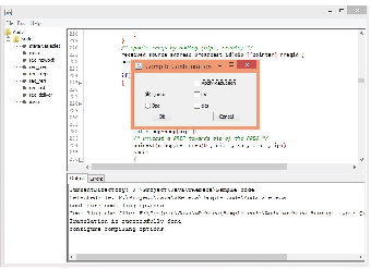
During state-space generation, information about the state variables and transitions are stored as an LTS in the Aldebaran format44 4 http://cadp.inria.fr/man/aldebaran.html. This LTS can be evaluated by tools such as the mCRL2 toolset [afra]. For example, one can express desired properties in -calculus [MS03] and verify them. Also, as explained in Section 5, labels are extended with network constraints as defined in [GFM11] so that the reduced LTS can be model checked with respect to underlying topology [GAFM13].
7.3 Model Checking of the AODV Protocol Properties
There are different ways to check a given property on a wRebeca model. Invariant properties can be evaluated while generating the state space by checking each reached global state against defined invariants. Furthermore, the resulting state space can be model checked by tools supporting Aldebaran format such as mCRL2 and CLTS model checker.
7.3.1 Checking the Loop Freedom Invariant
Loop freedom is one of the well-known property which must hold for all routing protocols such as the AODV protocol. For example, consider the routes to a destination in the routing tables of all nodes, where has a route to with the next hop , has a route to with the next hop , and has a route to with the next hop . The given example constructs a loop which consists of the three nodes, , , and . A state is considered loop free if the collective routing table entries of all nodes for each pair of a source and destination do not form a loop. As it was mentioned earlier in AODV-v2-11, each route may have more than one next hop when the adjacency states of the next hops are unconfirmed. Therefore, while the loop freedom of a state is checked, one must take into account all next hops stored for each route. Then, for each next hop check whether it leads to a loop or not. A routing protocol deployed on a network is called loop free if all of its reachable states are loop free. In other words, loop freedom property of a protocol is an invariant (which can be easily specified by the ACTL-X fragment of -calculus, and hence, is preserved by the reduced semantic model). However, We have extended our state-space generator engine to check invariants (specified by functions) over each newly generated global state on the fly by calling the functions provided by a user, i.e., the invariants. To this aim, we have specified the loop freedom invariant by a recursive function, to inspect for a given global state whether the next hops in the routing table entries of nodes collectively lead to a loop-formation scenario, as shown in Figure 19. Therefore, whenever the state-space generator reaches to a new state, before proceeding any further, it checks whether any loop is formed on the forward/backward routes between the source and destination, by calling and , as and are the destination and source respectively. If the loop freedom condition is violated, the function returns , and the state generator engine stops while it returns the path which has led to the global state under consideration as a counter example. The function has three parameters: refers to the destination of the route, refers to the IP address of the current node which is going to be processed and is the list of IP addresses of those nodes which have been processed.
Although keeping more than one next hop for each route may increase the route availability, it compromises its validity by violating the loop freedom invariant in a network of at least four nodes with a dynamic topology. Consider the network topology shown in Figure 2(a). The following scenario explains steps that lead to the invariant violation.
- 1.
initiates a route discovery procedure for destination by broadcasting a message.
- 2.
and upon receiving the message, add a route to their routing tables towards and store as their next hop. Since it is the first time that these nodes have received a message from , the neighbor state of is set to unconfirmed. Therefore, the route state is unconfirmed.
- 3.
As and are not the intended destination of the route request, they rebroadcast the message.
- 4.
receives the message sent by and since the route to is unconfirmed it adds as a new next hop to .
- 5.
also adds as the new next hop towards after processing the sent by . At this point a loop is formed between and .
- 6.
receives the message sent by and since it is the destination, it sends a message towards .
- 7.
moves out of the communication ranges of and .
- 8.
receives the message sent by and as the route state towards is unconfirmed it unicasts the message one by one to the existing next hops, and , till it gets an ack. Since has moved out of the communication ranges of , no ack is received from and gets removed from the routing table as the next hop to . Then, another is sent to . Since is adjacent to , it receives the message and then sends an ack to . Therefore, sets the neighbor state of to confirmed and subsequently the route state towards to valid.
- 9.
by receiving the message from unicasts it to its next hops and similar to . Since it fails to receive an ack from and receives one from , it updates its routing table by validating as its next hop to .
We have found the scenario in the wRebeca model with the network constraint resulting four topologies as indicated in Table 4. However, this scenario was also found for all the network constraints described in the table. Furthermore, we can generalize the scenario to all networks with the same connectivity when the communications occur, and the same mobility scenario.
7.3.2 Checking the Properties by mCRL2
Sequence numbers are used frequently by the AODV protocol to evaluate the freshness of routes. Therefore, it is important that each node’s sequence number increases monotonically. To this end, we manually configured the state generator to add two self-loops to each state with the label to monitor the sequence number of the source node, where is of the source node, and the label to trace the destination sequence number of routes to the source and destination for each node (i.e., the backward and forward routes to the destination of our model), where and are and of node , respectively. These properties are expressed through the ACTL-X fragment of -calculus as shown in Figure 20. The first formula asserts a monotonic increase of the source sequence number. The second formula assures the destination sequence numbers stored in the routing table of are increased monotonically, and must hold for the nodes in the model.
7.3.3 Checking Packet Delivery Property by the CLTS Model Checker
The CLTS model checker can be used to express and verify interesting properties of MANET protocols dependent to the underlying topology specified in Constrained Action Computation Tree Logic (CACTL) [GAFM13], an extension of Action CTL [DV90]. The path quantifier All in CACTL is parametrized by a multi-hop constrain over the topology, which specifies the pre-condition required for paths of a state to be inspected. Therefore, a state satisfies if its paths over which the multi-hop constraint holds, also satisfy . It also contains the two temporal operators until and weak until to specify the path formulae and to denote a path over which states satisfying are met by actions of until a state satisfying is met by actions of (in case of weak until, the state satisfying can never be met).
The important property of packet delivery in routing or information dissemination protocols in the context of MANETs becomes: if there exists an end-to-end route (multi-hop communication path) between two nodes and for a sufficiently long period of time, then packets sent by will eventually be received by [FVGH+13]. To specify such the property, inspired from [FVGH+13] we revised our specification to include data packet handling (to forward the packet to its next hop towards the destination) in addition to the route discovery packets and their corresponding handlers. Therefore, whenever a node, source, discovers a route to an intended destination, it starts forwarding its data packet through the next hop specified in its routing table. The data packet is forwarded by intermediate nodes to their next hops. When the data packet reaches the intended destination, it delivers the data to itself by unicasting the message to itself. In case an intermediate node fails to forward the message, the error recovery procedure is followed as explained in Section 6. Consequently, using the following formula, we can verify packet delivery property:
It expresses that as long as there is a stable multi-hop path from to and vice versa (specified by ), any message is proceeded by a message after passing -transitions which abstract away from other message communications. By model checking the resulting CLTS of the AODVv2 model, we found a scenario in which the property does not hold. We explain this scenario in a network of three nodes , and , where node is always connected to the nodes and , while the connection between the nodes and is transient. Therefore, the mobility of nodes leads to the topologies shown in Figure 10(b) and Figure 10(c). Assume the topology is initially as the one in Figure 10(b):
- •
Node unicasts a to itself, indicating that it wants to send to node .
- •
Node initiates a route discovery procedure by broadcasting an message to its neighbors, i.e., nodes and . Note that refers to an message received from node with the hop count of . Each message has more parameters but here only these two parameters are of interest and the other parameters are assumed to be equal for all the messages, i.e., the destination and source sequence numbers, and the source and destination IP addresses.
- •
Node processes the and since it is not the destination and has no route to in its routing table, rebroadcasts the message to its neighbors, nodes and , after increasing the hop count. At this point, node has two messages in its queue, and .
- •
Node moves out of the communication range of node , resulting the network topology shown in Figure 10(c).
- •
Node takes from the head of its queue and updates its routing table by setting as the next hop in the route towards . As node is the intended destination for the route discovery message, it unicasts an message towards the originator, , indicating that the route has been built and it can start forwarding the data. Therefore, node attempts to unicast an message to node , i.e., its next hop towards the originator.
- •
Since the connection between the nodes and is broken, it fails to receive an ack from and marks the route as invalid.
- •
Node takes from its queue and since the route state towards is invalid, it evaluates the received route to determine whether it is loop free. Updating the routing table with the received route is said to be “loop free”, if the received message cost, e.g., the hop count is less than or equal to the existing route cost. Since the hop count of the received message is greater than the existing one, it does not update the existing route and the message is discarded.
Although the route through node to node seems to be valid, the protocol refuses to employ it to prevent possible loop formation in the future.
8 Related Work
A large number of studies has been conducted for modeling and verification of MANET protocols using different approaches to tackle its specific challenges. These challenges, as discussed in Section 3, are modeling the underlying topology, mobility and local broadcast.
Some works model and analyze the correctness of MANET protocols using existing formal frameworks such as SPIN [DRA04, WPP04] and UPPAAL [FvGH+12, MF06, WPP05]. In a SPIN model, node connectivity is modeled with the help of PROMELA channels, one for each node. Also, mobility is modeled by case selection instruction provided by PROMELA, for modeling nondeterminism. In the initialization section, possible links to other neighbors are defined as different cases that all will be checked for a model. Since it does not provide a specific technique to reduce the state space, its state space grows very fast and it is only feasible to check small topologies. Therefore, models would be limited to fewer nodes. In UPPAAL, connectivity is modeled through a set of arrays of booleans, while changing topology is modeled by a separate automaton which manipulates the arrays. In [WPP04], a case study was carried out to evaluate two model checkers, SPIN and UPPAAL. Due to state-space explosion, the analysis was limited to some special mobility scenarios (as a part of the specification). However, our reduction technique makes it possible to verify a MANET for all possible topology changes to find an error.
As explained in [EM99], from a theoretical point view, compositionality is not preserved if broadcast is encoded based on point-to-point communications. Lack of support for compositional modeling and arbitrary topology changes has motivated new approaches with a primitive for local broadcast and support of arbitrary mobility in an algebraic way. These approaches include CBS# [NH06], CWS [MS06], CMN [Mer09], the -calculus [SRS10], bA [God10], CMAN [God07, God09], RBPT [GFM08] and the bpsi-calculi [BHJ+15, PBPR13]. Each of these proposed frameworks overcome the modeling difficulties such as local broadcast and its message delivery guarantee property and mobility in different ways. All these approaches, except CBS#, CWS, AWN and bpsi-calculi, suffer from lack of message delivery guarantee that makes them inappropriate for analyzing properties such as packet delivery [FVGH+13]. They model broadcast through either an enforced synchronized or lossy communication. When communications are lossy, a node may not receive a message although it is in the transmission range of the sender. CBS# and CWS use enforced synchronization for broadcast to make sure that all ready nodes within the transmission range of a sender will receive the message. Although they guarantee message delivery to the ready receivers, it is not possible to define meaningful nodes (which can successfully receive messages while they are processing another message) in their syntax which are always ready (i.e, input-enabled) [FVGH+13]. The process algebra AWN is proposed particularly for modeling wireless mesh network (WMN) routing protocols which uses local broadcast with message delivery guarantee. It defines its own data structures to model routing tables and other necessary data types to model the AODV protocol. In addition, conditional unicast is introduced for modeling the procedure to act based on the message delivery acknowledgment. In all these approaches, while a node is busy processing a message, it fails to receive messages from other nodes. Therefore, either nodes are defined to be input-enabled at the semantics as in CBS# and CWS or a process with a queue that concurrently stores new messages should be specified at the syntax as in AWN and bpsi-calculus. Almost all these languages model mobility of nodes in their semantics through arbitrary changes of the topology with the exception that it is modeled through different generations of assertions on connectivity information in [BHJ+15]. In wRebeca, communications are asynchronous and received messages are stored in queues implicitly at the semantic level (without the need to make nodes explicitly input-enabled). Furthermore, the atomic execution of message handlers, which avoids unnecessary interleaving of the node behaviors, together with topology abstraction through -elimination technique, where the topology changes are a source of state-space explosion in the process calculi approaches, make our framework applicable to the verification of real-world yet complex protocols such as AODV. We remark that unnecessary interleaving of behaviors can be handled in bpsi-calculus by means of priorities.
There are different approaches [DSTZ12, DSZ11, ADR+11] with the aim to analyze networks with an infinite number of nodes, where nodes execute an instance of a network process. A network configuration is represented as a graph in which each individual node represents a state of the process. The behavior of a process is modeled by an automaton. The network configuration transforms due to either the process evolution at a network node or the topology reconfiguration. Verification of safety properties, reaching to an undesirable configuration starting from an initial configuration, is parameterized due to any possible number of nodes and connectivity among them. It is proved that the problem of parameterized safety properties, the so-called control states reachability problem, is undecidable. However, that problem turns out to be decidable for the class of bounded path graphs [DSZ11, DSTZ12]. Decidability of the problem was also considered when configurations evolve due to discrete/continuous clocks at processes [ADR+11]. Furthermore, an inductive approach based on reduction to prove compositional invariants for the dynamic process networks was presented in [NT15a]. This approach reduces the calculation of a compositional invariant to a smallest representative network through setting up a collection of local symmetry relations between nodes, specifically defined for each problem. The computed non-dynamic compositional invariant on the representative network is generalized for the entire dynamic network family when the non-dynamic invariant is preserved by any reaction to a dynamic change in the network. Then, they proved loop freedom of AODVv2-04 for an arbitrary number of nodes in [NT15b] through an inductive and compositional proof: It provides an inductive invariant and proves that it is held initially and also preserved by every action, either a protocol action or a change in the network, similar to the approach of [vGHPT16]. They have reported two loop-formation scenarios due to inappropriate setting of timing constants and accepting any valid route when the current route is broken without any further evaluation (to ensure loop formation). Another approach is based on graph transformation systems, where network configurations are hypergraphs and transitions are specified by graph rewriting rules, modeling the dynamic behavior of a protocol. Safety properties are symbolically specified by graph patterns, a generalized form of hypergraphs with negative conditions, through a symbolic backward reachability analysis which is not guaranteed to terminate due to the undecidability of the problem [SWJ08]. To this aim, an over-approximation of the set of configurations preceding a bad configuration are computed by using a fixed point analysis, and then check that this set contains no initial configuration. While these approaches are scalable to prove a property for MANETs with a potentially unbounded number of nodes with an exhaustive effort, our approach is valuable to easily examine confirmation and diagnostics of suspected errors in the early phase of protocol development for a limited number of nodes. In other words, our efficient model checking tool can be used as an initial step before involving to generalize a property for an arbitrary sized network.
9 Conclusion and Future Work
In this paper we extended the syntax and semantics of bRebeca, the actor-based modeling language for broadcasting environment, to support wireless communication in a dynamic environment. We addressed the key features of wireless ad hoc networks, namely reliable local broadcast, conditional unicast, and last but not least mobility. The reliable asynchronous local broadcast/unicast communication, and implicit support of message storages make our framework suitable to analyze MANETs with respect to different mobility scenarios. A modeler only focuses on how to decompose a protocol into a set of communicating actors to cover functionalities of the protocol under investigation.
To overcome the state-space explosion, we leveraged the counter abstraction technique to analyze ad hoc networks with static topologies. Our reduction technique performs well on protocols with no specific state variable that distinguishes each rebec, and topologies with many topologically equivalent nodes. We demonstrated the effectiveness of our approach on the flooding protocol in different network settings. However, mobility ruins the soundness of our counting abstraction. To this end, we eliminated -transitions while topology information was removed from the global states to considerably reduce the size of the state space. We integrated the proposed reduction techniques into a tool customizable in verifying wRebeca models for different message storage policies and the topology dynamism. Invariants can be checked during the state-space generation while the resulting output can be fed into the existing model checking tools such as mCRL2 and CLTS model checker.
We presented a complete and accurate model of the core functionalities of a recent version of AODVv2 protocol (version 11). We abstracted optional features and timing aspects to make our model manageable. We verified the loop freedom property in AODVv2-11 and found a scenario in which the property violated. The scenario was confirmed by the AODV group. Loop freedom has already been proved on various versions of AODV: AODVv1-02 [BOG02], AODV-rfc3561 [FVGH+13, vGHPT16], and AODVv2-04 [NT15b, SWJ08], respectively. Among these only [NT15b] considers the timed behavior of the AODV. The new version differs in the following aspects which distinguish our attempt: in this version multiple next hops are maintained for each destination and consequently the process to update the routing table is completely different; Different statuses are considered for a route in the table of a node regarding the neighbor status of its next hop; Sequence numbers for invalid destinations in intermediate nodes are not increased anymore (like [NT15b, SWJ08], in contrast to others). Although, these approaches focus on providing a general proof for the property, our model checking-based approach detects the error and the scenario that leads to it. Our approach, can be adopted to resolve conceptual/design errors in an iterative way in the early phase of protocol development. The positive result of verifications constitutes a predicate about the protocol for a limited number of nodes. The combination of model checking and theorem proving techniques allows to prove a predicate about a MANET protocol for any number of nodes.
We plan to integrate our state-space generator tool into the verification environment [afrb] to take advantage of its model checker. Furthermore, we aim to run more cast studies to extend application of our framework. To analyze real-time and probabilistic behaviors of wireless network protocols, wRebeca can be extended in the same way of [KSS+15, VK12]. To this aim, there is a need to examine the soundness of our reduction techniques when probability and time are introduced.
Acknowledgements
We would like to thank the anonymous reviewers for their constructive comments on the earlier version of the paper, the AODV group for their supports, Mohammad Reza Mousavi for his discussion on the paper, Wan Fokkink and Bas Luttik for their helpful comments on the paper.
References
- [ADR+11] P. Aziz Abdulla, G. Delzanno, O. Rezine, A. Sangnier, and R. Traverso. On the verification of timed ad hoc networks. In 9th International Conference on Formal Modeling and Analysis of Timed Systems, volume 6919 of LNCS, pages 256–270. Springer, 2011.
- [afra] mCRL2: analysing system behaviors. http://www.mcrl2.org/.
- [afrb] Rebeca formal modeling language. http://www.rebeca-lang.org/wiki/pmwiki.php/Tools/Afra.
- [Agh90] Gul A. Agha. ACTORS - a model of concurrent computation in distributed systems. MIT Press series in artificial intelligence. MIT Press, 1990.
- [Beh] wRebeca, Efficient Modeling of Mobile Ad hoc Networks. https://github.com/b-yousefi/wRebeca.
- [BG92] D. P. Bertsekas and R.t G. Gallager. Data Networks. Prentice Hall, 1992.
- [BHJ+15] Johannes Borgström, Shuqin Huang, Magnus Johansson, Palle Raabjerg, Björn Victor, Johannes Åman Pohjola, and Joachim Parrow. Broadcast psi-calculi with an application to wireless protocols. Software and System Modeling, 14(1):201–216, 2015.
- [BMWK09] Gérard Basler, Michele Mazzucchi, Thomas Wahl, and Daniel Kroening. Symbolic counter abstraction for concurrent software. In Computer Aided Verification, pages 64–78. Springer, 2009.
- [BOG02] K. Bhargavan, D. Obradovic, and C. A. Gunter. Formal verification of standards for distance vector routing protocols. J. ACM, 49(4):538–576, 2002.
- [CCH07] Tao Cui, Lijun Chen, and Tracey Ho. Distributed optimization in wireless networks using broadcast advantage. In Decision and Control, pages 5839–5844. IEEE, 2007.
- [CEJS98] Edmund M. Clarke, E. Allen Emerson, Somesh Jha, and A. Prasad Sistla. Symmetry reductions in model checking. In Computer Aided Verification, pages 147–158. Springer, 1998.
- [DK86] R. Dechter and L. Kleinrock. Broadcast communications and distributed algorithms. IEEE Trans. Computers, 35(3):210–219, 1986.
- [DRA04] R De Renesse and AH Aghvami. Formal verification of ad-hoc routing protocols using spin model checker. In 12th IEEE Mediterranean, Electrotechnical Conference, volume 3, pages 1177–1182. IEEE, 2004.
- [DSTZ12] G. Delzanno, A. Sangnier, R. Traverso, and G. Zavattaro. On the complexity of parameterized reachability in reconfigurable broadcast networks. In Annual Conference on Foundations of Software Technology and Theoretical Computer Science, volume 18 of LIPIcs, pages 289–300. Schloss Dagstuhl - Leibniz-Zentrum fuer Informatik, 2012.
- [DSZ11] G. Delzanno, A. Sangnier, and G. Zavattaro. Parameterized verification of safety properties in ad hoc network protocols. In First International Workshop on Process Algebra and Coordination, volume 60 of EPTCS, pages 56–65, 2011.
- [DV90] R. De Nicola and F.W. Vaandrager. Action versus state based logics for transition systems. In Semantics of Systems of Concurrent Processes, volume 469 of Lecture Notes in Computer Science, pages 407–419. Springer, 1990.
- [EM99] C. Ene and T. Muntean. Expressiveness of point-to-point versus broadcast communications. In Fundamentals of Computation Theory, pages 258–268, 1999.
- [ET99] E. Allen Emerson and Richard J. Trefler. From asymmetry to full symmetry: New techniques for symmetry reduction in model checking. In Correct Hardware Design and Verification Methods, pages 142–156. Springer, 1999.
- [FvGH+12] Ansgar Fehnker, Rob van Glabbeek, Peter Höfner, Annabelle McIver, Marius Portmann, and WeeLum Tan. Automated analysis of AODV using Uppaal. In Tools and Algorithms for the Construction and Analysis of Systems, volume 7214 of LNCS, pages 173–187. Springer Berlin Heidelberg, 2012.
- [FVGH+13] Ansgar Fehnker, Rob Van Glabbeek, Peter Höfner, Annabelle McIver, Marius Portmann, and Wee Lum Tan. A process algebra for wireless mesh networks used for modelling, verifying and analysing AODV. arXiv preprint arXiv:1312.7645, 2013.
- [GAFM13] Fatemeh Ghassemi, Saeide Ahmadi, Wan Fokkink, and Ali Movaghar. Model checking MANETs with arbitrary mobility. In Fundamentals of Software Engineering, pages 217–232. Springer, 2013.
- [GFM08] F. Ghassemi, W. Fokkink, and A. Movaghar. Restricted broadcast process theory. In Sixth IEEE International Conference on Software Engineering and Formal Methods (SEFM), pages 345–354. IEEE Computer Society, 2008.
- [GFM11] F. Ghassemi, W. Fokkink, and A. Movaghar. Verification of mobile ad hoc networks: An algebraic approach. Theoretical Computer Science, 412(28):3262–3282, 2011.
- [God07] JensChr. Godskesen. A calculus for mobile ad hoc networks. In AmyL. Murphy and Jan Vitek, editors, Coordination Models and Languages, volume 4467 of LNCS, pages 132–150. Springer Berlin Heidelberg, 2007.
- [God09] J. Chr. Godskesen. A calculus for mobile ad-hoc networks with static location binding. Electr. Notes Theor. Comput. Sci., 242(1):161–183, 2009.
- [God10] JensChr. Godskesen. Observables for mobile and wireless broadcasting systems. In Coordination Models and Languages, volume 6116 of LNCS, pages 1–15. Springer Berlin Heidelberg, 2010.
- [Hew77] Carl Hewitt. Viewing control structures as patterns of passing messages. Artif. Intell., 8(3):323–364, 1977.
- [JSM+10] Mohammad Mahdi Jaghoori, Marjan Sirjani, Mohammad Reza Mousavi, Ehsan Khamespanah, and Ali Movaghar. Symmetry and partial order reduction techniques in model checking Rebeca. Acta Informatica, 47(1):33–66, 2010.
- [Kat11] Joost-Pieter Katoen. Model checking: One can do much more than you think! In Fundamentals of Software Engineering, pages 1–14. Springer, 2011.
- [KLN11] F. Kuhn, N. A. Lynch, and C. C. Newport. The abstract MAC layer. Distributed Computing, 24(3-4):187–206, 2011.
- [KSS+15] E. Khamespanah, M. Sirjani, Z. Sabahi-Kaviani, R. Khosravi, and M. Izadi. Timed rebeca schedulability and deadlock freedom analysis using bounded floating time transition system. Science of Computer Programming, 98:184–204, 2015.
- [Mer09] Massimo Merro. An observational theory for mobile ad hoc networks (full version). Information and Computation, 207(2):194 – 208, 2009. Special issue on Structural Operational Semantics (SOS).
- [MF06] AK Mclver and Ansgar Fehnker. Formal techniques for the analysis of wireless networks. In Second International Symposium on Leveraging Applications of Formal Methods, Verification and Validation, pages 263–270. IEEE, 2006.
- [MKKAR06] S. Ali Mahmud, Shahbaz Khan, Shoaib Khan, and H. Al-Raweshidy. A comparison of manets and wmns: commercial feasibility of community wireless networks and manets. In 1st International Conference on Access Networks. ACM, 2006.
- [MS03] Radu Mateescu and Mihaela Sighireanu. Efficient on-the-fly model-checking for regular alternation-free mu-calculus. Sci. Comput. Program., 46(3):255–281, 2003.
- [MS06] Nicola Mezzetti and Davide Sangiorgi. Towards a calculus for wireless systems. Electronic Notes in Theoretical Computer Science, 158(0):331 – 353, 2006.
- [NH06] Sebastian Nanz and Chris Hankin. A framework for security analysis of mobile wireless networks. Theor. Comput. Sci., 367(1-2):203–227, 2006.
- [NT15a] K. S. Namjoshi and R. J. Trefler. Analysis of dynamic process networks. In Tools and Algorithms for the Construction and Analysis of Systems, volume 9035 of LNCS, pages 164–178. Springer, 2015.
- [NT15b] K. S. Namjoshi and R. J. Trefler. Loop freedom in aodvv2. In Formal Techniques for Distributed Objects, Components, and Systems, volume 9039 of LNCS, pages 98–112, 2015.
- [PB99] Charles E. Perkins and Elizabeth M. Belding-Royer. Ad-hoc on-demand distance vector routing. In 2nd Workshop on Mobile Computing Systems and Applications, pages 90–100. IEEE Computer Society, 1999.
- [PBPR13] J. Åman Pohjola, J. Borgström, J. Parrow, and P. Raabjerg. Negative premises in applied process calculi. Technical report, Department of Information Technology, Uppsala University, 2013.
- [Pen08] Jun Peng. A new arq scheme for reliable broadcasting in wireless lans. IEEE Communications Letters, 12(2):146–148, 2008.
- [Plo81] G. D. Plotkin. A structural approach to operational semantics. Technical Report DAIMI FN-19, University of Aarhus, 1981.
- [PXZ02] Amir Pnueli, Jessie Xu, and Lenore D. Zuck. Liveness with (0, 1, infty)-Counter Abstraction. In 14th International Conference on Computer Aided Verification, CAV ’02, pages 107–122. Springer-Verlag, 2002.
- [RSA+14] Arni Hermann Reynisson, Marjan Sirjani, Luca Aceto, Matteo Cimini, Ali Jafari, Anna Ingólfsdóttir, and Steinar Hugi Sigurdarson. Modelling and simulation of asynchronous real-time systems using Timed Rebeca. Sci. Comput. Program., 89:41–68, 2014.
- [SJ11] Marjan Sirjani and Mohammad Mahdi Jaghoori. Ten years of analyzing actors: Rebeca experience. In Formal Modeling: Actors, Open Systems, Biological Systems, pages 20–56. Springer, 2011.
- [SK13] Hamideh Sabouri and Ramtin Khosravi. Delta modeling and model checking of product families. In Fundamentals of Software Engineering, pages 51–65. Springer, 2013.
- [SL04] W. Si and C. Li. RMAC: A reliable multicast MAC protocol for wireless ad hoc networks. In 33rd International Conference on Parallel Processing (ICPP 2004), pages 494–501. IEEE Computer Society, 2004.
- [SMSdB04] Marjan Sirjani, Ali Movaghar, Amin Shali, and Frank S. de Boer. Modeling and verification of reactive systems using Rebeca. Fundam. Inform., 63(4):385–410, 2004.
- [SRS10] Anu Singh, C.R. Ramakrishnan, and Scott A. Smolka. A process calculus for mobile ad hoc networks. Science of Computer Programming, 75(6):440 – 469, 2010. 10th International Conference on Coordination Models and Languages COORD’08.
- [SS10] Hamideh Sabouri and Marjan Sirjani. Slicing-based reductions for rebeca. Electronic Notes in Theoretical Computer Science, 260:209–224, 2010.
- [SWJ08] M. Saksena, O. Wibling, and B. Jonsson. Graph grammar modeling and verification of ad hoc routing protocols. In 14th International Conference on Tools and Algorithms for the Construction and Analysis of Systems, volume 4963 of LNCS, pages 18–32. Springer, 2008.
- [vGHPT16] R. J. van Glabbeek, P. Höfner, M. Portmann, and W. Lum Tan. Modelling and verifying the AODV routing protocol. To appear in Distributed Computing, 2016.
- [vGW96] R. van Glabbeek and W. P. Weijland. Branching time and abstraction in bisimulation semantics. Journal of the ACM, 43(3):555–600, 1996.
- [VK12] Mahsa Varshosaz and Ramtin Khosravi. Modeling and verification of probabilistic actor systems using pRebeca. In Formal Methods and Software Engineering, pages 135–150. Springer, 2012.
- [WPP04] Oskar Wibling, Joachim Parrow, and Arnold Pears. Automatized verification of ad hoc routing protocols. In Formal Techniques for Networked and Distributed Systems, volume 3235 of LNCS, pages 343–358. Springer, 2004.
- [WPP05] Oskar Wibling, Joachim Parrow, and Arnold Pears. Ad hoc routing protocol verification through broadcast abstraction. In Formal Techniques for Networked and Distributed Systems-FORTE 2005, pages 128–142. Springer, 2005.
- [YGK15] B. Yousefi, Fatemeh Ghassemi, and Ramtin Khosravi. Modeling and efficient verification of broadcasting actors. In In pre-proceeding of 6th IPM International Conference on Fundamentals of Software Engineering, pages 114–128, 2015.