Optimal Estimation of Slope Vector in
High-dimensional Linear Transformation Model
Abstract
In a linear transformation model, there exists an unknown monotone nonlinear transformation function such that the transformed response variable and the predictor variables satisfy a linear regression model. In this paper, we present CENet, a new method for estimating the slope vector and simultaneously performing variable selection in the high-dimensional sparse linear transformation model. CENet is the solution to a convex optimization problem and can be computed efficiently from an algorithm with guaranteed convergence to the global optimum. We show that under a pairwise elliptical distribution assumption on each predictor-transformed-response pair and some regularity conditions, CENet attains the same optimal rate of convergence as the best regression method in the high-dimensional sparse linear regression model. To the best of our limited knowledge, this is the first such result in the literature. We demonstrate the empirical performance of CENet on both simulated and real datasets. We also discuss the connection of CENet with some nonlinear regression/multivariate methods proposed in the literature.
Key Words: canonical correlation analysis, elastic net penalty, elliptical distribution, Kendall’s tau, optimal rate of convergence, variables transformation.
1 Introduction
Recently, there has been significant interest in theoretically appealing and algorithmically efficient regression methods that are suitable for analyzing high-dimensional datasets whose dimension is comparable or much larger than the sample size . Under the linear regression model, researchers have proposed various computationally efficient regularization methods for simultaneously estimating the slope vector and selecting predictors, and substantial progress has been made on understanding the theoretical properties of these regression methods. See, for example, Tibshirani (1996); Chen et al. (1998); Fan and Li (2001); Efron et al. (2004); Zou and Hastie (2005); Zou (2006); Candes and Tao (2007); Bickel et al. (2009); Bühlmann and van de Geer (2011) and the references therein. In particular, when is assumed to be sparse with number of non-zero coordinates , the lasso estimator and the Dantzig selector have been shown to both attain an optimal rate of convergence for estimating (Bickel et al., 2009).
When the relationship between the response variable and the predictors is nonlinear, however, the performance of regression methods based on linear models can be severely compromised. In this paper, we study a family of sparse transformational regression models where a response variable is related to predictor variables through an equation
| (1) |
Here is an unknown, strictly increasing transformation function, is a sparse slope vector of interest, and is a noise term independent of with unknown distribution . Model (1) generalizes the linear regression model by allowing an unknown monotone transformation on the response variable . It has been widely studied in the classical setting, but the problem of estimating in model (1) in the high-dimensional setting has received much less attention and a rate of convergence has not been derived. Han and Wang (2015) recently proposed a rank-based estimator for and established consistency but not rate of convergence of their estimator. Furthermore, the algorithm for computing their estimator does not scale well with increasing dimension and sample size. In this paper, we propose a computationally efficient method for estimating in the high-dimensional setting, given independent and identically distributed observations from (1). Since is unknown, for identifiability of the model we assume that and satisfy and throughout the paper, where . Interestingly, we showed that under certain regularity conditions, our estimator achieves a convergence rate of for estimating . To the best of our limited knowledge, this is the first result in the literature that shows that an estimator for model (1) achieves the same optimal rate of convergence as the best regression method in the sparse linear regression model, despite the unknown nonlinearity introduced by .
Model (1) is also known as the linear transformation model (Doksum, 1987; Dabrowska and Doksum, 1988) and has been studied extensively in the literature in the low-dimensional setting. It generates many popular econometric and statistical models under different assumptions on and . For example, when takes the form of a power function and is a normal distribution, model (1) reduces to the familiar Box-Cox transformation models (Box and Cox, 1964; Bickel and Doksum, 1981). On the other hand, model (1) specializes to the Cox’s proportional hazard model (Cox, 1972) and the proportional odds rate model (Pettitt, 1982; Pettitt, 1984; Bennett, 1983) when denotes the extreme value distribution and the standard logistic distribution, respectively. More general models for which is unknown and is specified up to a vector of finite-dimensional parameter were studied in Doksum (1987); Dabrowska and Doksum (1988); Cheng et al. (1995); Chen et al. (2002), among others. In the case where there are no parametric specifications for both the transformation function and the noise distribution, Han (1987) introduced the maximum rank correlation (MRC) estimator for , treating as a nuisance parameter. Given an estimate of , Horowitz (1996), Ye and Duan (1997), Klein and Sherman (2002), and Chen (2002) further proposed methods for estimating . The MRC approach is based on the idea of maximizing a rank-based correlation between and . Rank estimation is known to be robust, and retains a relatively high level of efficiency. However, due to the discontinuity of the rank-based objective function in the MRC approach, the computation of the MRC estimator is intractable especially in high dimensions. In addition, such a discontinuity renders the theoretical analysis of the MRC estimator difficult. Lin and Peng (2013) proposed a computationally simpler smoothing approach as a remedy to the drawbacks of the MRC procedure, and established the -consistency and asymptotic normality of their estimator. A more recent work by Han and Wang (2015) offered a similar approach and extended the study of the estimation problem to the high-dimensional setting. In fact, the model considered in Han and Wang (2015) is a more general model than (1), and was first introduced in Han (1987) under which the MRC estimator is also applicable. Although Han and Wang (2015) characterized the range of the problem dimensions for which their estimator is consistent, they did not establish the convergence rate of their estimator. Moreover, their algorithm requires substantial running time for large and/or and only finds local optimums.
Another line of work that is related to model (1) is based on the idea of sufficient dimension reduction. In this framework, is assumed to be independent of conditional on the projection of onto some lower-dimensional subspaces. The goal is then to recover the effective dimension reduction (e.d.r.) space, which is the minimal subspace for which the conditional independence property holds. Model (1) can be viewed as a special case in this framework where the e.d.r. space of interest is one-dimensional. Many methods have been proposed in the context of sufficient dimension reduction (Cook and Weisberg, 1991; Li, 1992; Cook, 1998), but the sliced inverse regression (SIR) method of Duan and Li (1991) is the first, yet the most widely studied method. Although SIR can be applied to model (1), the original implementation of SIR proposed by Duan and Li (1991) requires to be smaller than . While several proposals extending SIR to the high-dimensional setting have appeared in the literature (Li and Yin, 2008; Yu et al., 2013; Lin et al., 2015), the rate of convergence of SIR in high dimensions has not yet been derived. In particular, Li and Yin (2008) proposed SIR with both - and -regularization but did not study the theoretical properties of their method. Yu et al. (2013) proposed to combine SIR with the Dantzig selector (Candes and Tao, 2007) and established a non-asymptotic rate for the recovery of the e.d.r. space, but the sparsity is not allowed to scale with and in their theoretical guarantees. A more recent paper by Lin et al. (2015) proposed to apply a preliminary variables screening procedure before fitting SIR. Lin et al. (2015) gave a consistency result for their method in the high-dimensional setting, but again, a rate of convergence has not been established.
In this paper, we propose the Constrained Elastic Net (CENet), a new method that combines a robust rank correlation and an elastic net penalty for performing simultaneous estimation and variable selection in the linear transformation model (1) in the high-dimensional setting. Our proposal is inspired by the correspondence between least squares regression and (one-dimensional) canonical correlation analysis (CCA), and is conceptually simple. CENet is the solution of a convex optimization problem and hence can be computed efficiently. We showed that under certain regularity conditions, the CENet estimator achieves the optimal convergence rate of . Our convergence rate is established from a random- point of view, under a pairwise elliptical assumption on the distribution of each predictor and the transformed response. We do not make any assumptions on besides it being strictly increasing. In addition to robustness to nonlinearity in the response, our simulation results also indicate the robustness of CENet to heavy-tailed noise distribution. Finally, we show that a connection exists between CENet and SIR, and also two other nonlinear multivariate techniques proposed in the literature: the alternating conditional expectation (ACE) method of Breiman and Friedman (1985) and the additive principal components (APC) method of Donnell et al. (1994). Such an observation adds new insight to the understanding of behavior of SIR, ACE, and APC under model (1).
1.1 Related Models
When is strictly increasing, model (1) belongs to the class of single-index models:
| (2) |
This can be seen by noting the equivalence between model (1) and
where is the inverse transformation, in which case and . In general, is different from due to the integration with respect to the noise distribution.
The single-index model is well-studied in low dimensions. Some important proposals for estimating the slope vector include the semiparametric -estimation approaches (Ichimura, 1993; Härdle et al., 1993; Delecroix et al., 2006) and the average derivative estimation approaches (Härdle and Stoker, 1989; Powell et al., 1989; Hristache et al., 2001). The -estimators have been shown to possess nice theoretical properties such as consistency and asymptotic efficiency. Nonetheless, they are rarely implemented in practice as they involve solving difficult non-convex optimization problem. The average derivative estimators can be computed directly, but they involve local smoothing and yield worse performance as the dimension increases due to data sparseness (the so-called “curse of dimensionality”). Another drawback for both the -estimators and the average derivative estimators is that they usually require strong smoothness assumptions on .
In the high-dimensional setting, Alquier and Biau (2013) provided a PAC-Bayesian analysis for single index models in the case where is sparse. Plan et al. (2014) and Plan and Vershynin (2015) proposed metrically projected marginal regression estimators and generalized Lasso estimators, respectively, in the case where lies in some known low-dimensional subspace . They showed that by exploiting the structural assumptions on , these estimators attain fast rates of convergence despite the unknown nonlinearity in observations. However, the clean theoretical results of Plan et al. (2014) and Plan and Vershynin (2015) are established under the assumption that follows a multivariate normal distribution, and it is unclear if similar results hold at a greater generality. Radchenko (2015) proposed a promising approach for sparse single index models that does not require such a restrictive assumption on . Nonetheless, the theoretical analysis requires boundedness on , smoothness on , and subgaussianity of , and the convergence rate of the proposed estimator is not as fast as ours.
1.2 Organization
The remainder of the paper is organized as follows. In Section 2, we introduce our new methodology CENet, discuss the intuition behind it, and present an efficient algorithm for computing it. We study the performance of CENet in Section 3. In Section 3.1, we establish the rate of convergence of CENet. We conduct some simulation studies to evaluate the finite-sample performance of CENet in Section 3.2. Section 3.3 gives a real data application of CENet. We conclude with Section 4, where we give a detailed description of the connection of CENet with SIR, ACE, and APC. The proofs of the theoretical results in Section 3.1 are collected in Appendix A. Appendix B contains the proofs of all other results in the paper, while Appendix C contains the derivation details of our algorithm. More extensive simulation results can be found in Appendix D.
Notation:
For any event , denotes its indicator function. For a vector , we denote the , , , and (pseudo)-norms of by , , , and , respectively. For a matrix , its spectral norm is given by . The notation stands for the index set for a positive integer . For any set , denotes its cardinality and denotes its complement. For any subsets , , we use to represent the submatrix of with rows and columns indexed by and . For a symmetric matrix , we write to indicate that is positive semidefinite. For any , denotes its principal square root that is positive semidefinite and satisfies . The notation and stand for the smallest and the largest eigenvalue of , respectively. We write for the identity matrix and for the vector of all zeros (the respective dimension of which will be clear from context). For any , we set . Finally, , and variants thereof denote generic positive constants whose value may vary for each occurrence.
2 Methodology
In this section, we introduce CENet for estimation of in the linear transformation model. We are particularly interested in the setting where the dimension can be much larger than the sample size . In such a setting, it is common to assume that is sparse, i.e., contains many zero entries.
2.1 The Optimization Problem
Throughout the paper, we assume model (1) holds and we observe independent and identically distributed pairs generated from (1), where and . We do not pose any parametric assumptions on the transformation function , except that it being strictly monotonically increasing. Let and . Since is unknown, for identifiability of the model we assume that any additive and multiplicative constants are absorbed into , so that and . Without loss of generality, we also assume that .
In practice, when is known, then can be found as the solution to
Since is generally unknown, cannot be estimated through a direct least squares approach. However, there is a direct correspondence between least squares regression and (one-dimensional) CCA:
Proposition 1.
Suppose that model (1) holds. Then is a solution to
| (3) |
In other words, among all linear combinations with , has the highest correlation with . Note that is only identifiable up to scale in (3). The following lemma gives an alternative formulation of (3), where with is the unique solution:
Lemma 1.
Solving (3) is equivalent to solving the following CCA problem:
| (4) |
To obtain an estimator for , a simple idea is to replace and in (4) with their empirical estimates and , and solve the resulting optimization problem. However, such an approach is problematic in two respects: (1) without knowledge of , is not estimable; (2) the sample covariance matrix is a natural estimator for but is singular when , so there might exist infinitely many solutions to such an empirical version of (4).
To address the first issue, we note that for ,
where , , and . To estimate , we use , the sample standard deviation of . To estimate , we exploit the monotonic assumption on and consider the use of Kendall’s tau, a classical nonparametric correlation estimator. The Kendall’s tau statistic is defined as
| (5) |
Note that the Kendall’s tau statistic is invariant under strictly monotone transformations of ’s and ’s. The population version of Kendall’s tau is given by
where the second equality holds under the assumption that is strictly monotonically increasing.
One can show that Kendall’s tau is related to Pearson correlation through
| (6) |
when follows a multivariate normal distribution (see, e.g., Cramér (1946), p. 290), or, more generally, a joint elliptical distribution (Lindskog et al., 2003). Motivated by such a relationship, we propose to estimate by the transformed version of Kendall’s tau:
| (7) |
We then define as our “estimator” for , with entry given by
| (8) |
Remark 1.
Since is only identifiable up to scale, there is no need to estimate . Without loss of generality, we can set in (8) to 1.
We wish to estimate in the case , and also to induce sparsity on our estimator . To address the second issue of singularity of , we propose to solve the following constrained optimization problem:
| (9) |
Here we turn the optimization problem (4) into a convex problem and we regularize the optimization criterion by an elastic net penalty (Zou and Hastie, 2005), where and are tuning parameters. We refer to the solution to (9) as CENet, standing for Constrained Elastic Net.
The formulation (9) of CENet is inspired by the formulation of the CCA problem in Gao et al. (2014). Different from the CCA formulation in Gao et al. (2014) which only employs an -penalty, in (9) an additional -penalty is needed because of the use of the robust estimator . In such a case, when , is singular and there might exist vectors belonging to the null space of that are not orthogonal to , such that the criterion in (9) with is unbounded below. Indeed, the following lemma gives a sufficient condition for the existence and uniqueness of solution to problem (9) across all values of and . The key is that ensures that we have a strictly convex criterion.
Lemma 2.
Suppose that and . Then there exists a unique solution to problem (9).
The following lemma, on the other hand, gives the range of for which .
Lemma 3.
The solution to (9) is completely sparse if and only if .
Hence, when selecting , we need never consider a value larger than that in Lemma 3.
2.2 ADMM Algorithm for CENet
Although (9) is a convex problem, closed form solution is not available. We consider using the Alternating Direction Method of Multipliers (ADMM) to solve (9) (Boyd et al., 2011).
We first rewrite the optimization problem as follows:
| (10) |
where
Then the augmented Lagrangian of (10) takes the form
where is an ADMM parameter. We present the ADMM algorithm for solving (9) in Algorithm 1. Derivations of the algorithm can be found in Appendix C.
- (1)
Initialize , , .
- (2)
Repeat:
- (a)
update for (solving a lasso problem):
where
- (b)
update for (projection onto the unit ball):
- (c)
update for :
- (d)
;
until .
- (a)
3 Performance of CENet
In this section, we study the performance of CENet. We first give our main results in Section 3.1, where we establish the rate of convergence of CENet under some regularity conditions. In Section 3.2, we explore the finite-sample performance of CENet through simulation studies. Finally, we demonstrate an application of CENet on a real dataset in Section 3.3.
3.1 Rate of Convergence
We first state the main assumptions used to establish the rate of convergence of CENet.
Assumption 1.
For , is pairwise elliptical.
Under model (1), Assumption 1 holds, for instance, when follows a joint elliptical distribution. Such an assumption is sufficient for (6) to hold (Lindskog et al., 2003). We examine the sensitivity of CENet to violations of Assumption 1 in Section 3.2.
Remark 2.
More generally, Kendall (1949) showed that when a bivariate random variable is not normal but the Pearson correlation exists, an approximation of the Kendall’s tau using the bivariate Gram-Charlier series expansion up to the fourth-order cumulants yield
where , , are bivariate cumulants. This means that we may expect (6) to be approximately true even in some cases where Assumption 1 is violated.
The following subgaussian assumption on and boundedness condition on are adopted to ensure that a restricted eigenvalue condition holds with high probability for . The restricted eigenvalue condition is a key assumption used in bounding the estimation error of lasso-type estimators in the high-dimensional sparse linear regression model (Bickel et al., 2009; Bühlmann and van de Geer, 2011).
Assumption 2.
- (i)
is subgaussian, with subgaussian norm , where ;
- (ii)
There exists a positive constant such that .
Remark 3.
Assumptions 1 and 2(i) are satisfied when is multivariate normal. More generally, suppose that follows a mixture variance normal distribution, i.e., , where is a constant vector, and is a scalar random variable independent of . Suppose further that almost surely, where is some constant. Then is joint elliptical and is subgaussian, and so Assumptions 1 and 2(i) are also satisfied.
We now state our main results:
Theorem 1.
Consider the linear transformation model (1) with true slope vector satisfying . Suppose that Assumptions 1 and 2 hold, and
| (11) |
for some sufficiently large constant . For any constant , there exists positive constants , and depending only on , and , such that when the tuning parameters for and ,
with probability at least .
Since the linear transformation model contains the linear regression model as a special case, the rate in Theorem 1 is optimal. The following is an immediate consequence of Theorem 1:
Corollary 1.
Under the same conditions as in Theorem 1, for any constant , there exist positive constants , and depending only on , and , such that when for and ,
with probability at least .
3.2 Simulation Studies
We study the finite-sample performance of CENet in this section. Due to the use of Kendall’s tau, we expect CENet to be robust to both nonlinear monotone transformations on the response variable and heavy-tailed noise distributions. In addition, we are interested in the sensitivity of CENet to violations of Assumption 1 in Section 3.1. We examine these issues in the following simulation studies. For comparison, we also evaluate the performance of the lasso and the smoothed MRC estimator of Han and Wang (2015) in our simulation studies. More extensive simulation results can be found in Appendix D.
Simulation settings:
We consider two scenarios for the transformation function:
The first scenario concerns the linear model whereas the second scenario concerns a linear transformation model. For each scenario, we generate data according to model (1) with , with , and we sample independent of from one of the following distributions:
- (a)
normal: ;
- (b)
contaminated normal: , ;
- (c)
mixture normal: ;
- (d)
centralized gamma: , where , .
Each of the (uncontaminated) noise distribution above has mean 0 and variance . We calibrate to achieve a desired level of . Under such a data generating mechanism, Assumption 1 is not satisfied except for noise distribution (a).
Figure 1 shows the densities for each of the four noise distributions. Compared to the normal distribution which is unimodal and symmetric, the contaminated normal distribution has heavier tails whereas the mixture normal distribution is bimodal and the gamma distribution is skewed.
Performance measures:
For fair comparison of different methods, we assess the performance of an estimator by the standardized squared estimation error
In the case , we simply set the estimation error as . Each method we consider has a tuning parameter that controls the sparsity of ( for CENet, for lasso and MRC). We compute the estimation error as a function of the number of non-zero coordinates of .
To measure the accuracy of support recovery for , we also consider plotting the receiver operating characteristic (ROC) curves, which is the plot of the true positive rate (TPR) against the false positive rate (FPR):
TPR gives the proportion of nonzero elements in that are correctly estimated to be nonzero, whereas FPR gives the proportion of zero elements in that are incorrectly estimated to be nonzero.
Implementation details:
For each scenario and noise distribution, we generate 100 simulated datasets with dimension and sample size (high-dimensional setting), (low-dimensional setting). For CENet, we fix , or and consider a range of . In all numerical results reported in this section, we set the ADMM parameter and the tolerance level in Algorithm 1. We implement the smoothed MRC estimator using the code provided by the authors. MRC requires the specification of a smoothing function and corresponding smoothing parameter value. We choose a Gaussian CDF approximation and use its default smoothing parameter value, and consider a range of . For lasso, we use the implementation given in the R-package gam (Hastie, 2015) and consider a range of .
Results:
Since both CENet and MRC are invariant to monotone transformation of the response variable , we combine the results for scenarios 1 and 2 in Figures 2 and 3. Figure 2 shows the results for each method under different noise distributions, when , and . The panels on the left column correspond to the plots of average squared estimation error (MSE) over average number of non-zero coordinates of estimated slopes, while the panels on the right column correspond to the average ROC curves. When the noise term follows a contaminated normal distribution, CENet performs the best while lasso performs the worst under both scenarios 1 and 2. Like CENet, MRC is much more robust to contaminated normal noise than lasso. Note that under both scenarios, the lasso estimated slopes tend to be dense. Moreover, the MSE is large and the estimation error curves stay relatively flat across different sparsity levels of the estimated slopes. It is therefore not surprising that lasso also has poor variable selection performance under the contaminated normal noise distribution. For other noise distributions, when the estimated slope is sparse, CENet has comparable MSE to lasso under scenario 1, and it has much smaller MSE than lasso (under scenario 2) and MRC (under both scenarios). Similarly, the variable selection performance of CENet is comparable to lasso under scenario 1, and is consistently better than lasso under scenario 2 and MRC under both scenarios. For all noise distributions, we also see that the overall estimation and variable selection performance of CENet improves as gets smaller. Based on our limited simulation experience, we recommend when each predictor variable is standardized to have unit variance.
Although MRC is designed for the high-dimensional setting, we see from Figure 2 that its MSE curves are quite flat and take relatively large values compared to CENet when , across all noise distributions. A plot of its MSE against tuning parameter (see Figure in Appendix D) suggests that MRC suffers from convergence issue in such a low signal-to-noise ratio setting. As we increase the sample size to , we see from Figure 3 that the convergence issue dissipates. The estimation error curves of MRC first decrease then increase with respect to the number of non-zero coordinates of estimated slopes, just like those of all other methods (except for lasso under the contaminated normal noise). The estimation performance of MRC improves significantly compared to when . We observe similar improvement when is increased from 0.6 to 0.9 (see Appendix D). Under the contaminated normal noise distribution, CENet still performs the best and lasso still performs the worst under both scenarios. For other noise distributions, CENet and MRC perform comparably to lasso under scenario 1 and outperform lasso under scenario 2 in terms of estimation. CENet performs much better than MRC in terms of variable selection. Interestingly, the performance of lasso under scenario 2 is not as bad as one might have anticipated when the noise distribution is not heavy-tailed. We also observe that when , the performance of CENet is relatively insensitive to the values of .
In summary, CENet has comparable performance to lasso under the linear model, but is considerably more robust to heavy-tailed noise distributions in both the linear and the transformation model. Moreover, it is not too sensitive to the underlying noise distributions when the noise is sampled independently from the predictors. Its performance improves as becomes smaller. On the other hand, MRC is reasonably robust to both non-linearity in the response variable and heavy-tailed noise distributions, but it does not perform as well as CENet in all the cases we consider, unless the signal-to-noise ratio is high.
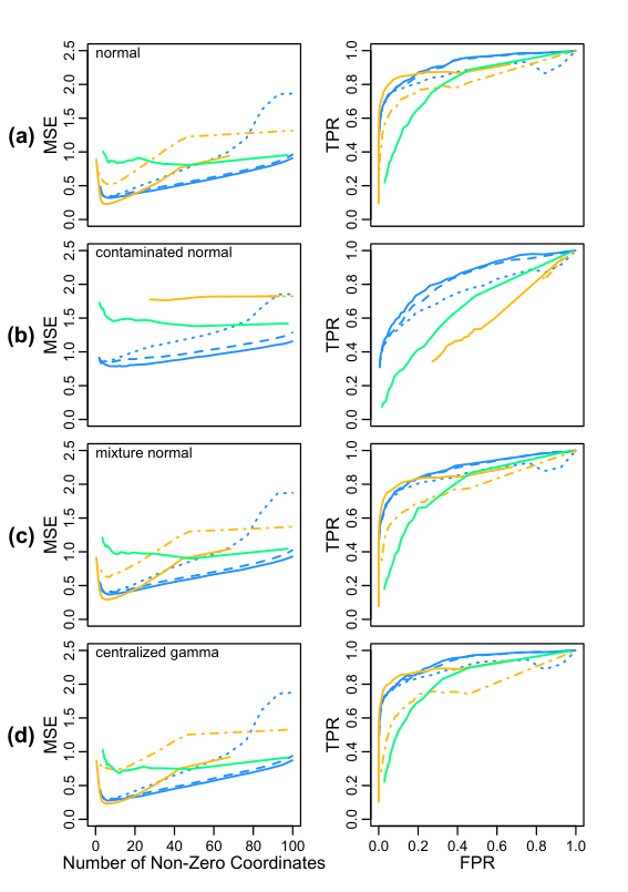
 ), lasso under scenario 2 (
 ), CENet with (
 ), (
), ( ), (
), ( ) under both scenarios, and MRC (
 ) under both scenarios.
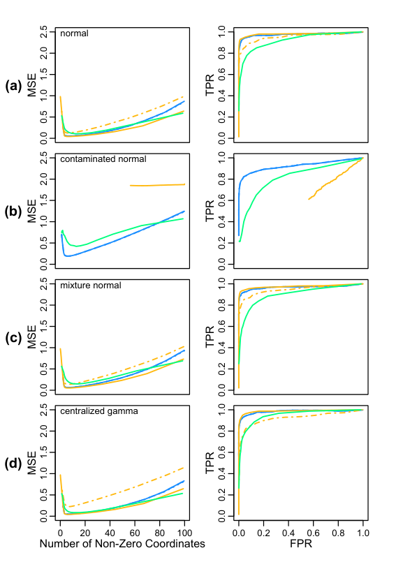 ), lasso under scenario 2 (), CENet with (), (), () under both scenarios, and MRC () under both scenarios.
3.3 Data Application
We consider the cardiomyopathy microarray data from a transgenic mouse model of dilated cardiomyopathy that is related to the understanding of human heart diseases (Redfern et al., 2000). The dataset includes an matrix of gene expression values , where is the expression level of the gene for the mouse, for and . Each mouse also give an outcome expression level of a G protein-coupled receptor, designated Ro1.
The cardiomyopathy microarray data was previously studied in Segal et al. (2003), Hall and Miller (2009), and Li et al. (2012). The goal is to determine genes whose expression changes are due to the expression of Ro1. However, such a selection is inherently difficult due to two distinguishing features of the microarray data: (i) vastly exceeds , and (ii) the gene expression values are highly correlated. Segal et al. (2003) gave an overview and evaluation of some proposals for tackling these issues, and obtained results that motivate regularized regression procedures such as the lasso and the least angle regression (Efron et al., 2004) as alternate regression tools for microarray studies. As noted in Segal et al. (2003), a major challenge with the application of these high-dimensional regression methods is the determination of the right amount of regularization.
In this study, we do not argue whether regularized regression procedures are the best tools for analyzing the cardiomyopathy microarray data. Instead, we are interested in exploring whether there is a significant overlap between the genes selected by CENet and those that are identified in Segal et al. (2003), Hall and Miller (2009), and Li et al. (2012). We address the problem of proper regularization with the stability selection of Meinshausen and Bühlmann (2010). We first standardize the expression values of each gene to have zero mean and unit variance. We then repeat for times:
- (i)
Sample pairs of with replacement from the original dataset.
- (ii)
Since , we apply the robust rank correlation based screening procedure of Li et al. (2012) to the resampled dataset and retain the top 50 genes that have the highest Kendall’s tau correlation (in magnitude) with the Ro1 expression values. Li et al. (2012) showed that for the purpose of variable selection it is appropriate to perform variables screening before fitting a linear transformation model, as the screening step will eliminate irrelevant predictors and keep relevant predictors with high probability. A similar screening strategy based on sample correlation has been widely used in practice when fitting a linear regression model, and a theoretical justification can be found in Fan and Lv (2008).
- (iii)
Apply CENet with over a grid of , and record the genes selected (i.e., genes whose corresponding ) for each .
Finally, we compute , the selection frequency of the gene across the B resampled datasets at tuning parameter value , for at each value. Figure 4 shows the stability path of each gene, which is the plot of against for . There are five genes that stand out throughout their stability paths (colored in red): Msa.10108.0, Msa.10044.0, Msa.1009.0, Msa.1166.0, Msa.10274.0. Besides for Msa.1166.0, none of the other four genes have been previously implicated for the cardiomyopathy dataset. Msa.1166.0 was identified in Hall and Miller (2009) and Li et al. (2012) for its strong nonlinear association with the Ro1 expression level. A second group of genes stand out when , and their stability paths are colored in blue: Msa.7019.0, Msa.2877.0, Msa.5794.0, Msa.15442.0. We highlighted the stability paths of a third group of genes in green, as they also stand out, albeit less strongly, when : Msa.1590.0, Msa.2134.0, Msa.3969.0. The genes Msa.7019.0, Msa.2877.0, Msa.2134.0 were identified in Li et al. (2012) for their high Kendall’s tau correlations with the Ro1 expression level.
For comparison, we also compute the stability paths of lasso for the cardiomyopathy dataset. We follow essentially the same steps as outlined above for CENet, except that we use Pearson correlation rather than Kendall’s tau for variables screening, and we apply lasso over . From Figure 5, we see that four genes stand out throughout their stability paths (colored in red): Msa.2877.0, Msa.964.0, Msa.778.0_i, Msa.2134.0. Besides for Msa.964.0, the other three genes have been previously identified by Segal et al. (2003) using lasso with cross-validation. We also see that four other genes stand out when (colored in blue): Msa.1590.0, Msa.1043.0, Msa.3041.0, Msa.741.0. Msa.1590.0 is also identified by CENet when .
Surprisingly, we do not see an overlap between the top five genes identified by CENet and the top four genes identified by lasso, though it is known (Li et al., 2012) that Msa.1166.0 identified by CENet is highly collinear with Msa.2877.0 identified by lasso. Upon inspection, we find that the relative strengths of association between the expression level of each of these nine genes and that of Ro1 change when the measure of association is changed from Pearson correlation to Kendall’s tau. For instance, the two genes Msa.964.0 and Msa.778.0_i stand out when the association is measured by Pearson correlation, but they do not stand out when the association is measured by Kendall’s tau. Figures 6 and 7 show the scatterplots of expression level of each of these nine genes with the Ro1 expression level. In such a case, Pearson correlation measures the strength of linear relationship between the gene expression level and the Ro1 expression level. For comparison, we also include the scatterplots of the ranked gene expression levels, which serve to illustrate the strengths of association as measured by Kendall’s tau. We see that the association is better captured by Kendall’s tau for Msa.10274.0 and Msa.1166.0 (i.e., the scatterplots of ranked expression levels exhibit more linearity than their unranked counterparts), whereas the association is better captured by Pearson correlation for Msa.2134.0 and Msa.2877.0 (i.e., the scatterplots of original expression levels exhibit more linearity than their ranked counterparts).
Due to the relatively small sample size (), it is hard to justify if there is a single best way to summarize the association between the expression level of Ro1 and that of other genes. As was mentioned in Segal et al. (2003), with the current state of microarray technology and study dimensions, different data processing and/or modeling approaches can give very different results. This is not necessarily a bad thing as such results can be viewed from a “sensitivity analysis” perspective, and ultimately, microarray results need to be validated experimentally by another complimentary method. The interpretation of the biological relevance of the genes identified above is beyond the scope of the paper. For completeness, we include their names and descriptions in Table 1.

 ), Msa.7019.0, Msa.2877.0, Msa.5794.0, Msa.15442.0 (
 ), and Msa.1590.0, Msa.2134.0, Msa.3969.0 (
 ).
). ), and Msa.1590.0, Msa.1043.0, Msa.3041.0, Msa.741.0 ().

| Genes | Descriptions |
|---|---|
| Msa.10108.0 | Homologous to sp P07814: MULTIFUNCTIONAL AMINOACYL-TRNA SYNTHETASE |
| Msa.10044.0 | Homologous to sp P10658: PROBABLE PHOSPHOSERINE AMINOTRANSFERASE |
| Msa.1009.0 | Mouse myoblast D1 (MyoD1) mRNA, complete cds |
| Msa.1166.0 | Mus musculus sterol carrier protein-2 (SCP-2) gene, complete cds |
| Msa.10274.0 | Homologous to sp P07335: CREATINE KINASE, B CHAIN |
| Msa.7019.0 | Homologous to sp P10719: ATP SYNTHASE BETA CHAIN, MITOCHONDRIAL PRECURSOR |
| Msa.2877.0 | Mouse MARib mRNA for ribophorin, complete cds |
| Msa.5794.0 | Homologous to sp P11730: CALCIUM/CALMODULIN-DEPENDENT PROTEIN KINASE TYPE II GAMMA CHAIN (CAM- KINAS |
| Msa.15442.0 | Homologous to sp P07379: PHOSPHOENOLPYRUVATE CARBOXYKINASE, CYTOSOLIC (GTP) |
| Msa.1590.0 | Mouse protein kinase C delta mRNA, complete cds |
| Msa.2134.0 | Murine mRNA for 4F2 antigen heavy chain |
| Msa.3969.0 | Homologous to sp P36542: ATP SYNTHASE GAMMA CHAIN, MITOCHONDRIAL PRECURSOR |
4 Discussion
Nonlinear transformation of variables is commonly practiced in regression analysis. In the mainstream statistical literature, variables transformation methods have been introduced by way of an estimation problem based on a model with parameters and noise terms (Box and Cox, 1964; Carroll and Ruppert, 1984). The CENet method proposed in this paper and many other methods referenced in Section 1 fall into this category. Another line of work focuses on dimension reduction rather than approximation of regression surfaces, and an early important work is the sliced inverse regression (SIR) method of Duan and Li (1991). Yet a different approach towards nonlinear regression analysis exists, where one searches for optimal nonlinear transformation of variables through optimizing some objective function of interest, with or without a model in mind. This includes, in particular, the alternating conditional expectation (ACE) algorithm proposed by Breiman and Friedman (1985). Although the ACE algorithm is a powerful and useful tool, it is more of a nonlinear multivariate analysis method than a regression method (Buja, 1990), and is known to be connected to the additive principal components (APC) method of Donnell et al. (1994). Despite the fact that CENet is developed with model (1) in mind, interestingly we are able to find a connection between CENet and SIR, ACE, APC. Such a connection stems primarily from the fact that a correlation-based approach is used for all these methods, and that we take a random- view when motivating the CENet methodology.
4.1 Connections between CENet and SIR, ACE, APC
The inquiry of connections between CENet and SIR, ACE, APC is motivated by the key observation in Proposition 1 that is used to formulate CENet. Setting aside the fact that relation (6) (whose validity requires distributional assumption on ) is used to bypass the unknown nonlinear transformation in model (1), on a population level CENet is built on the simple idea of performing CCA on and , allowing linear transformation on each. Such an observation naturally links CENet to SIR, ACE, and APC, three methods that we will review in the next few paragraphs.
In their pioneering article on dimension reduction, Duan and Li (1991) considered a semiparametric index model of the form
| (12) |
where is an unknown link function and is a noise term independent of , and proposed SIR for estimating the effective dimension reduction (e.d.r.) space, which is the linear space generated by the ’s. Rather than modeling the conditional distribution of given as in conventional approaches, Duan and Li (1991) took an inverse modeling perspective by treating as random and considering the conditional distribution of given . Indeed, when , the population version of SIR amounts to solving the following generalized eigenproblem:
| (13) |
Chen and Li (1998) later showed that there is a natural connection between SIR and multiple linear regression, in that the SIR direction obtained from (13) can be interpreted as the slope vector of multiple linear regression applied to an optimally transformed . That is, the solution to (13) also solves
| (14) |
where the maximization is taken over all transformations with and vectors . Regarding the statistical theory of SIR, Duan and Li (1991) showed that the SIR directions fall into the e.d.r. space under a linearity assumption on the distribution of , which is satisfied when follows an elliptical distribution. Observing that model (1) is a special case of model (12) for which SIR is applicable, that both SIR and CENet require some sort of (elliptical) distributional assumption on for recovering , and also comparing (3) and (14), it is natural to expect that a connection exists between SIR and CENet.
The characterization (14) of SIR in terms of maximum correlation connects it to ACE (Breiman and Friedman, 1985) and APC (Donnell et al., 1994; Tan et al., 2015), two nonlinear multivariate techniques that make use of maximum correlation for searching optimal variable transformations. Given a response and predictors , Breiman and Friedman (1985) considered a regression model of the form , and defined the optimal ACE transformations as functions that solve
Whereas each predictor is allowed to make only linear transformation in SIR, each is allowed to make possibly nonlinear transformation in ACE. When have a joint normal distribution and is an independent , and , for (Breiman and Friedman, 1985, p. 581).
On the other hand, APC treats all variables symmetrically by fitting an implicit additive equation , as opposed to regression analysis which treats variables asymmetrically by singling out a response variable. The (smallest) APC transformations can be found by solving
In the case where , the smallest and the largest APCs (obtained by maximizing instead of minimizing the criterion above) are in trivial correspondence since a largest APC given by generates a smallest APC given by .
In general, APC and ACE analyses are not identical, but a direct correspondence exists in one-simple situation: single-predictor ACE is equivalent to two-variable APC (Donnell et al., 1994, Section 4.6). Such an equivalence enables us to link SIR to APC, by treating and as the two variables of interest, and considering linear transformation for and possibly nonlinear transformation for . The following lemma summarizes the connection among SIR, ACE, and APC.
Proposition 2.
SIR, ACE, and APC are equivalent in that
| (15) |
Remark 4.
In (15) we replace the infinite-dimensional Hilbert spaces in ACE by a single -dimensional Hilbert space and keep the same. On the other hand, in APC we take for the two variables and and consider optimizing over and . In essence, one can view SIR as performing CCA between the Hilbert spaces and , and all three criteria in (15) are equivalent characterization of the CCA problem.
Now that we have established the equivalence of SIR, ACE, and APC (without referring to any true underlying models), we are ready to explore their connection with CENet. For brevity, in the rest of the section we shall refer to the solution to (15) as the SIR transformation and the SIR direction, respectively. Comparing (14) with (3), we see that to draw a connection between SIR and CENet, it suffices to find conditions for which the SIR transformation is (up to intercept and scale) when model (1) holds. The following proposition gives two such conditions:
Proposition 3.
Under model (1), suppose that is invertible, has mean 0 and variance , and that one of the following holds:
- (i)
follows a joint elliptical distribution with ;
- (ii)
is degenerate, i.e., (no distributional assumption on ).
Then the solutions to (15) recover and in model (1). In other words, the SIR direction obtained from (15) also solves (3).
Condition (i) includes the special case where has a multivariate normal distribution and independent of . Under condition (i), both the CENet direction and the SIR direction are proportional to . However, the validity of CENet relies on the relationship between the orthant probability and , whereas the validity of SIR relies on the linearity of the conditional expectation . Interestingly, when is invertible, has a joint elliptical distribution, and is independent of , then the SIR direction is always proportional to regardless of the distribution of (Duan and Li, 1991). However, in such a case the SIR transformation is not necessarily given by . On the other hand, the CENet direction will be affected by the distribution of even if is independent of , but the relation (6) (and hence, CENet) is valid under condition (i) even when . Although SIR is applicable to the more general model (12) and requires less restrictive assumption on the noise distribution than CENet, as mentioned in the introduction its rate of convergence in the high dimensions has not been derived, whereas CENet is shown to attain the optimal rate of convergence under a pair-elliptical assumption on , .
Under condition (ii), SIR recovers in model (1) regardless of the distribution of . This is not surprising given the equivalence of SIR with (14). Unfortunately, for CENet, an additional assumption like ellipticality of the distribution of is required for recovering even if is degenerate. This is because such an assumption is critical for us to bypass the estimation of in model (1), and the convenience comes at a price. On the contrary, the explicit need to estimate in (15) grants greater flexibility on the distribution of for SIR/ACE/APC, but it also renders their implementations more cumbersome and their theoretical analyses more challenging. Even if one considers computing the SIR direction from (13) where estimation of is not needed, the slicing step (Duan and Li, 1991) involved in estimating can still affect the finite-sample performance of SIR when is large relative to (even if ) due to data sparseness.
To summarize, we have the following corollary:
Corollary 2.
Remark 5.
Under conditions given in Corollary 2, unlike SIR, ACE, and APC, CENet recovers without requiring knowledge of .
4.2 Concluding Remarks
We have presented a new approach, CENet, for efficiently performing simultaneous variables selection and slope vector estimation in the linear transformation model when the dimension can be much larger than the sample size . CENet is the solution of a convex optimization problem, for which a computationally efficient algorithm with guaranteed convergence to the global optimum is provided. CENet has two tuning parameters that control the level of regularization. We showed that under certain regularity conditions, CENet attains the optimal rate of convergence for the estimation of slope vector in the sparse linear transformational models, just as the best regression method do in the sparse linear models. On the other hand, CENet does not require the specification of the transformation function and the noise distribution, and so is considerably more robust compared to existing estimation and variable selection methods for linear models in the large--small- setting. The robustness of CENet to both nonlinearity in the response and heavy-tailedness in the noise distribution is confirmed by the theoretical results and simulation studies given in the paper. We also showed that a connection exists between CENet and three other nonlinear regression/multivariate methods: SIR, ACE, APC, when model (1) is valid and an elliptical assumption on holds. In such a case, an advantage of CENet over SIR, ACE, and APC is that it bypasses the need to explicitly estimate the unknown transformation function when the primary interest is in the estimation of the slope vector.
The rate of convergence of the CENet estimator in the paper is established under an elliptical assumption on the predictor-transformed-response pairs. As demonstrated in our simulation results, CENet performs well when the noise term is generated independently of the predictor but not necessarily from the same family of distribution. This motivates studying the convergence rate of CENet when the pair-elliptical assumption is violated, and exploring if there exists more general condition for which CENet still attains the optimal rate of convergence. We leave this for future work.
Acknowledgements
We thank Fang Han and Honglang Wang for providing R code for implementing the MRC estimator proposed in Han and Wang (2015); Mark Segal for sharing the cardiomyopathy dataset studied in Segal et al. (2003); Andreas Buja, Zijian Guo, Po-Ling Loh, and Zongming Ma for helpful feedback that has helped improve the presentation of the paper.
References
- Alquier and Biau (2013) Alquier, P. and Biau, G. (2013), Sparse single-index model, J. Mach. Learn. Res. 14, 243–280.
- Bennett (1983) Bennett, S. (1983), Analysis of survival data by the proportional odds model, Statistics in medicine 2(2), 273–277.
- Bickel and Doksum (1981) Bickel, P. J. and Doksum, K. A. (1981), An analysis of transformations revisited, J. Amer. Statist. Assoc. 76(374), 296–311.
- Bickel et al. (2009) Bickel, P. J., Ritov, Y. and Tsybakov, A. B. (2009), Simultaneous analysis of lasso and Dantzig selector, Ann. Statist. 37(4), 1705–1732.
- Box and Cox (1964) Box, G. E. P. and Cox, D. R. (1964), An analysis of transformations. (With discussion), J. Roy. Statist. Soc. Ser. B 26, 211–252.
- Boyd et al. (2011) Boyd, S., Parikh, N., Chu, E., Peleato, B. and Eckstein, J. (2011), Distributed optimization and statistical learning via the alternating direction method of multipliers, Foundations and Trends® in Machine Learning 3(1), 1–122.
- Breiman and Friedman (1985) Breiman, L. and Friedman, J. H. (1985), Estimating optimal transformations for multiple regression and correlation, J. Amer. Statist. Assoc. 80(391), 580–619. With discussion and with a reply by the authors.
- Bühlmann and van de Geer (2011) Bühlmann, P. and van de Geer, S. (2011), Statistics for high-dimensional data, Springer Series in Statistics, Springer, Heidelberg. Methods, theory and applications.
- Buja (1990) Buja, A. (1990), Remarks on functional canonical variates, alternating least squares methods and ACE, Ann. Statist. 18(3), 1032–1069.
- Candes and Tao (2007) Candes, E. and Tao, T. (2007), The Dantzig selector: statistical estimation when is much larger than , Ann. Statist. 35(6), 2313–2351.
- Carroll and Ruppert (1984) Carroll, R. J. and Ruppert, D. (1984), Power transformations when fitting theoretical models to data, J. Amer. Statist. Assoc. 79(386), 321–328.
- Chen and Li (1998) Chen, C.-H. and Li, K.-C. (1998), Can SIR be as popular as multiple linear regression?, Statist. Sinica 8(2), 289–316.
- Chen et al. (2002) Chen, K., Jin, Z. and Ying, Z. (2002), Semiparametric analysis of transformation models with censored data, Biometrika 89(3), 659–668.
- Chen (2002) Chen, S. (2002), Rank estimation of transformation models, Econometrica 70(4), 1683–1697.
- Chen et al. (1998) Chen, S. S., Donoho, D. L. and Saunders, M. A. (1998), Atomic decomposition by basis pursuit, SIAM J. Sci. Comput. 20(1), 33–61.
- Cheng et al. (1995) Cheng, S. C., Wei, L. J. and Ying, Z. (1995), Analysis of transformation models with censored data, Biometrika 82(4), 835–845.
- Cook (1998) Cook, R. D. (1998), Principal Hessian directions revisited, J. Amer. Statist. Assoc. 93(441), 84–100. With comments by Ker-Chau Li and a rejoinder by the author.
- Cook and Weisberg (1991) Cook, R. D. and Weisberg, S. (1991), Comment, J. Amer. Statist. Assoc. 86(414), 328–332.
- Cox (1972) Cox, D. R. (1972), Regression models and life-tables, J. Roy. Statist. Soc. Ser. B 34, 187–220. With discussion by F. Downton, Richard Peto, D. J. Bartholomew, D. V. Lindley, P. W. Glassborow, D. E. Barton, Susannah Howard, B. Benjamin, John J. Gart, L. D. Meshalkin, A. R. Kagan, M. Zelen, R. E. Barlow, Jack Kalbfleisch, R. L. Prentice and Norman Breslow, and a reply by D. R. Cox.
- Cramér (1946) Cramér, H. (1946), Mathematical Methods of Statistics, Princeton Mathematical Series, vol. 9, Princeton University Press, Princeton, N. J.
- Dabrowska and Doksum (1988) Dabrowska, D. M. and Doksum, K. A. (1988), Partial likelihood in transformation models with censored data, Scand. J. Statist. 15(1), 1–23.
- Delecroix et al. (2006) Delecroix, M., Hristache, M. and Patilea, V. (2006), On semiparametric -estimation in single-index regression, J. Statist. Plann. Inference 136(3), 730–769.
- Doksum (1987) Doksum, K. A. (1987), An extension of partial likelihood methods for proportional hazard models to general transformation models, Ann. Statist. 15(1), 325–345.
- Donnell et al. (1994) Donnell, D. J., Buja, A. and Stuetzle, W. (1994), Analysis of additive dependencies and concurvities using smallest additive principal components, Ann. Statist. 22(4), 1635–1673. With a discussion by Bernard D. Flury [Bernhard Flury] and a rejoinder by the authors.
- Duan and Li (1991) Duan, N. and Li, K.-C. (1991), Slicing regression: a link-free regression method, Ann. Statist. 19(2), 505–530.
- Efron et al. (2004) Efron, B., Hastie, T., Johnstone, I. and Tibshirani, R. (2004), Least angle regression, Ann. Statist. 32(2), 407–499. With discussion, and a rejoinder by the authors.
- Fan and Li (2001) Fan, J. and Li, R. (2001), Variable selection via nonconcave penalized likelihood and its oracle properties, J. Amer. Statist. Assoc. 96(456), 1348–1360.
- Fan and Lv (2008) Fan, J. and Lv, J. (2008), Sure independence screening for ultrahigh dimensional feature space, J. R. Stat. Soc. Ser. B Stat. Methodol. 70(5), 849–911.
- Gao et al. (2014) Gao, C., Ma, Z. and Zhou, H. H. (2014), Sparse cca: Adaptive estimation and computational barriers, arXiv preprint arXiv:1409.8565 .
- Hall and Miller (2009) Hall, P. and Miller, H. (2009), Using generalized correlation to effect variable selection in very high dimensional problems, J. Comput. Graph. Statist. 18(3), 533–550.
- Han (1987) Han, A. K. (1987), Nonparametric analysis of a generalized regression model. The maximum rank correlation estimator, J. Econometrics 35(2-3), 303–316.
- Han and Wang (2015) Han, F. and Wang, H. (2015), Provable smoothing approach in high dimensional generalized regression model, arXiv preprint arXiv:1509.07158 .
- Härdle et al. (1993) Härdle, W., Hall, P. and Ichimura, H. (1993), Optimal smoothing in single-index models, Ann. Statist. 21(1), 157–178.
- Härdle and Stoker (1989) Härdle, W. and Stoker, T. M. (1989), Investigating smooth multiple regression by the method of average derivatives, J. Amer. Statist. Assoc. 84(408), 986–995.
- Hastie (2015) Hastie, T. (2015), ‘Gam: generalized additive models. r package version 1.12’.
- Horowitz (1996) Horowitz, J. L. (1996), Semiparametric estimation of a regression model with an unknown transformation of the dependent variable, Econometrica 64(1), 103–137.
- Hristache et al. (2001) Hristache, M., Juditsky, A. and Spokoiny, V. (2001), Direct estimation of the index coefficient in a single-index model, Ann. Statist. 29(3), 595–623.
- Ichimura (1993) Ichimura, H. (1993), Semiparametric least squares (SLS) and weighted SLS estimation of single-index models, J. Econometrics 58(1-2), 71–120.
- Kendall (1949) Kendall, M. G. (1949), Rank and product-moment correlation, Biometrika 36, 177–193.
- Klein and Sherman (2002) Klein, R. W. and Sherman, R. P. (2002), Shift restrictions and semiparametric estimation in ordered response models, Econometrica 70(2), 663–691.
- Li et al. (2012) Li, G., Peng, H., Zhang, J. and Zhu, L. (2012), Robust rank correlation based screening, Ann. Statist. 40(3), 1846–1877.
- Li (1992) Li, K.-C. (1992), On principal Hessian directions for data visualization and dimension reduction: another application of Stein’s lemma, J. Amer. Statist. Assoc. 87(420), 1025–1039.
- Li and Yin (2008) Li, L. and Yin, X. (2008), Sliced inverse regression with regularizations, Biometrics 64(1), 124–131, 323.
- Lin and Peng (2013) Lin, H. and Peng, H. (2013), Smoothed rank correlation of the linear transformation regression model, Comput. Statist. Data Anal. 57, 615–630.
- Lin et al. (2015) Lin, Q., Zhao, Z. and Liu, J. S. (2015), On consistency and sparsity for sliced inverse regression in high dimensions, arXiv preprint arXiv:1507.03895 .
- Lindskog et al. (2003) Lindskog, F., Mcneil, A. and Schmock, U. (2003), Kendall’s tau for elliptical distributions, Springer.
- Meinshausen and Bühlmann (2010) Meinshausen, N. and Bühlmann, P. (2010), Stability selection, J. R. Stat. Soc. Ser. B Stat. Methodol. 72(4), 417–473.
- Pettitt (1984) Pettitt, A. (1984), Proportional odds models for survival data and estimates using ranks, Applied Statistics pp. 169–175.
- Pettitt (1982) Pettitt, A. N. (1982), Inference for the linear model using a likelihood based on ranks, J. Roy. Statist. Soc. Ser. B 44(2), 234–243.
- Plan and Vershynin (2015) Plan, Y. and Vershynin, R. (2015), The generalized lasso with non-linear observations, arXiv preprint arXiv:1502.04071 .
- Plan et al. (2014) Plan, Y., Vershynin, R. and Yudovina, E. (2014), High-dimensional estimation with geometric constraints, arXiv preprint arXiv:1404.3749 .
- Powell et al. (1989) Powell, J. L., Stock, J. H. and Stoker, T. M. (1989), Semiparametric estimation of index coefficients, Econometrica 57(6), 1403–1430.
- Radchenko (2015) Radchenko, P. (2015), High dimensional single index models, J. Multivariate Anal. 139, 266–282.
- Redfern et al. (2000) Redfern, C. H., Degtyarev, M. Y., Kwa, A. T., Salomonis, N., Cotte, N., Nanevicz, T., Fidelman, N., Desai, K., Vranizan, K., Lee, E. K. et al. (2000), Conditional expression of a gi-coupled receptor causes ventricular conduction delay and a lethal cardiomyopathy, Proceedings of the National Academy of Sciences 97(9), 4826–4831.
- Segal et al. (2003) Segal, M. R., Dahlquist, K. D. and Conklin, B. R. (2003), Regression approaches for microarray data analysis, Journal of Computational Biology 10(6), 961–980.
- Tan et al. (2015) Tan, X. L., Buja, A. and Ma, Z. (2015), Kernel additive principal components, arXiv preprint arXiv:1511.06821 .
- Tibshirani (1996) Tibshirani, R. (1996), Regression shrinkage and selection via the lasso, J. Roy. Statist. Soc. Ser. B 58(1), 267–288.
- Vershynin (2012) Vershynin, R. (2012), Introduction to the non-asymptotic analysis of random matrices, in ‘Compressed sensing’, Cambridge Univ. Press, Cambridge, pp. 210–268.
- Ye and Duan (1997) Ye, J. and Duan, N. (1997), Nonparametric -consistent estimation for the general transformation models, Ann. Statist. 25(6), 2682–2717.
- Yu et al. (2013) Yu, Z., Zhu, L., Peng, H. and Zhu, L. (2013), Dimension reduction and predictor selection in semiparametric models, Biometrika 100(3), 641–654.
- Zou (2006) Zou, H. (2006), The adaptive lasso and its oracle properties, J. Amer. Statist. Assoc. 101(476), 1418–1429.
- Zou and Hastie (2005) Zou, H. and Hastie, T. (2005), Addendum: “Regularization and variable selection via the elastic net” [J. R. Stat. Soc. Ser. B Stat. Methodol. 67 (2005), no. 2, 301–320; mr2137327], J. R. Stat. Soc. Ser. B Stat. Methodol. 67(5), 768.