The discrete sign problem: uniqueness, recovery algorithms and phase retrieval applications

Consider a signal ${\bf F}\in\mathbb{R}^{N}$ satisfying assumptions A1 and A2, and further assume that the length $\tau$ of the compact support of $\bf f$ is a-priori known. As in our earlier works [24, 25], instead of working with the $(\tau+1)$ signal values $f(k)$, $k=-\tau/2,\ldots,\tau/2\,(\!\!\!\!\mod N)$, as the unknown variables, we consider the vector of $N$ unknown signs ${\bf X}=(X_{0},\ldots,X_{N-1})$. Further, rather than dealing with the combinatorial set ${\bf X}\in\{-1,1\}^{N}$, we relax this constraint and allow all entries $X_{j}$ to be complex valued, namely ${\bf X}\in\mathbb{C}^{N}$.

As we now show, this allows us to write a system of linear equations for the vector ${\bf X}$ over the field $\mathbb{C}$ whose unique real-valued solution is the true sign pattern. The first set of equations captures the compact support assumption on the vector ${\bf f}={\mathcal{D}FT}\{{\bf F}\}$. Since ${\bf f}$ is zero outside the set of indices CS of Eq. (5), the unknown vector ${\bf X}$ must satisfy the following set of $N-\tau-1$ linear equations

The second set of equations imposes the known segmentation into intervals of constant sign, as described in A2. Let $\mathcal{S}$ denote the set of indices within the intervals of constant sign, excluding the last one in each interval. Then,

Given a segmentation to $M$ constant sign intervals the number of equations in (7) is thus $N-M$.

By definition, the true sign pattern ${\bf s}=sign({\bf F})$ is a solution of Eqs. (6)-(7). Theorem 3 below shows that under suitable conditions and up to multiplication by a constant, it is the only solution to this system of equations.

By Theorem 3, with a suitable over-segmentation one can retrieve the sign of $\bf F$ by solving the set of linear equations (6)-(7). To this end, however, one must first determine an (over-)segmentation from $|{\bf F}|^{2}$ alone. The following lemma provides a principled method to do so.

Lemma 2 implies that at any pair of consecutive indices $\{j-1,j\}$ that satisfy

the sign of $\bf F$ must be equal. Hence, knowing only the vector $|{\bf F}|$, Eq. (9) provides an over-segmentation to constant sign intervals. If the number of found segments $M$ is sufficiently small so that $N>2\tau+M$ then we can directly recover the sign pattern by solving the system of linear equations (6)-(7).

Unfortunately, even though Eq. (9) provides a correct over-segmentation, with a finite over-sampling rate the resulting number of segments can be too large, so that the corresponding Eqs. (6)-(7) have multiple solutions. To decrease the number of segments, and thus increase the number of linear equations, we supplement Eq. (9) with a heuristic segmentation scheme which works very well in practice, even though it is not theoretically guaranteed to yield a correct over-segmentation. Our heuristic segmentation scheme relies on the fact that for a sign change to occur between ${F}_{j}$ and ${F}_{j+1}$ its analytic continuous extension $F(\omega)$ must have a zero crossing at some intermediate $\omega\in[\omega_{j},\omega_{j+1}]$. Hence, $|{\bf F}|$ is likely to have a local discrete minimum near this zero crossing.

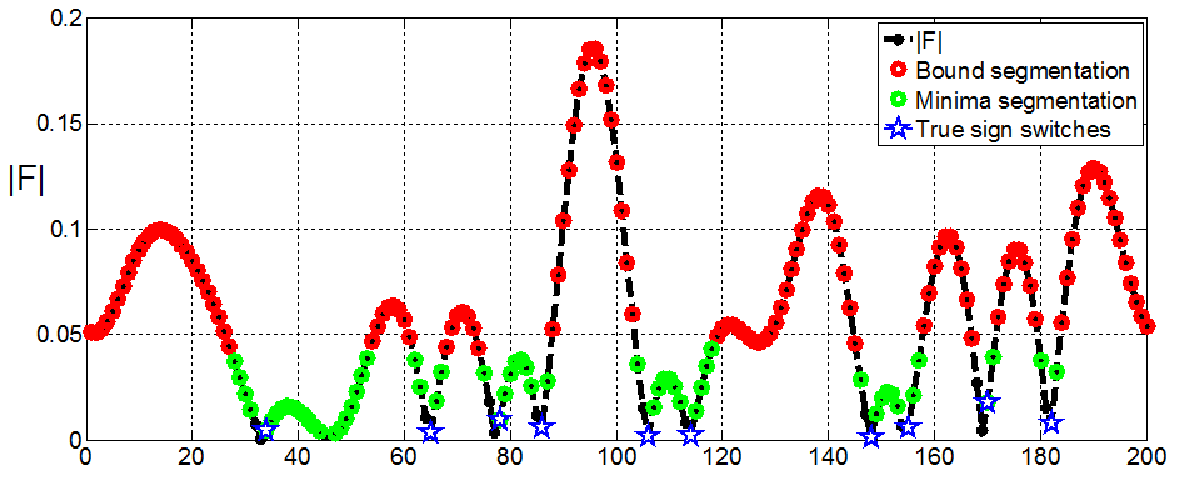
This observation leads to the following segmentation algorithm summarized in Table 1: First, the discrete local minima of $|{\bf F}|$ are found and their indices are defined as single index segments. Next, all the indices between each pair of consecutive minima are defined to have the same sign. Finally, for each minimum index, the adjacent index for which $|{\bf F}|$ has closer value to the minimum value is also defined as a single index segment. The last step is applied to reduce errors in the resulting segmentation. In the absence of noise, our final segmentation is the merging of both segmentations described above. Fig. 9 in Section 6.6 presents an example of the segmentations produced by both schemes.

In any realistic scenario the vector of intensities $|{\bf F}|^{2}$ is measured with some noise. In this case, no sign pattern satisfies Eq. (6). To cope with measurement noise, we reformulate the sign problem as the minimization of a suitable quadratic functional. To this end, we first describe our noise model, then construct the functional to be minimized and detail our minimization approach.

Let $|\tilde{\bf F}|^{2}$ be the vector of noisy measurements. As described in [25], a rather general noise model is

where ${\bm{\eta}}^{s}$ is background additive noise with noise level $\sigma$, ${\bm{\eta}}^{d}$ is dark counts noise, and $|{\bf F}+{\tfrac{\sigma}{\sqrt{N}}}{\bm{\eta}}^{s}|{\bm{\eta}}^{sh}$ is the detector shot noise which is proportional to the signal intensity. In many cases the dark counts ${\bm{\eta}}^{d}$ has small variance and its main effect can be removed by proper calibration. We thus assume for simplicity that ${\bm{\eta}}^{d}=0$. We assume a classical light experiment, far from the single photon regime and we thus neglect the effect of shot noise. We further assume that ${\bm{\eta}}^{s}=(\eta^{s}_{0},\ldots,\eta^{s}_{N-1})$ consists of $N$ independent and identically distributed (i.i.d.) complex-valued Gaussian random variables $\mathcal{N}(0,1)$.

To cope with noisy measurements, we modify our sign retrieval scheme in two ways: (i) refine the method to find an oversegmentation; (ii) replace the solution of a homogeneous linear system by the minimization of a quadratic functional. In the presence of noise, our sign retrieval consists of the following key steps:

Next, we impose our two segmentation schemes starting with the heuristic one. We use $\mathcal{S}_{1}$ to construct the matrix $\mathcal{A}_{1}$ of size $S_{1}\times N$, whose $k^{th}$ row is given by

where $k\in[1,S_{1}]$, $l_{k}$ is the $k$-th index in ${\cal S}_{1}$, and the vector of weights ${\bf W}=[W_{1},\dots,W_{S_{1}}]$ is defined as $W(k)=\min\{|{\tilde{F}}_{l_{k}}|^{2},|{\tilde{F}}_{l_{k}+1}|^{2}\}$. We note that $\mathcal{A}_{1}{\bf X}=0$ imposes that $\bf X$ is piecewise constant in the intervals defined by Table 1. The purpose of $\bf W$ is to account for the fact that the heuristic algorithm presented in Table 1 does not guarantee a correct over-segmentation and that errors typically occur at indices corresponding to low $|\tilde{\bf F}|^{2}$ values where we have less certainty in our segmentation. With our weighting approach, we have that $\mathcal{A}_{1}{\bf X}=0$ imposes $W_{j}(X_{j}-X_{j+1})=0$ for $j\in\mathcal{S}_{1}$. Hence, when a quadratic functional based on $\mathcal{A}_{1}$ is minimized, as described below, the constraint that $\bf X$ is piecewise constant at $j\in\mathcal{S}_{1}$ is suppressed for entries corresponding to low $|\tilde{\bf F}|^{2}$ values.

Our second segmentation approach is guaranteed to yield a correct over-segmentation in the noise-free case, and in practice for high SNR, it is unlikely to make errors. Hence, we impose this segmentation without weights, in a way that also reduces the computational cost of our problem by reducing the number of variables. To this end, we sum over the appropriate columns of the $(N+S_{1}-\tau-1)\times N$ matrix $[\mathcal{A}_{cs};\mathcal{A}_{1}]$ to construct the matrix $\mathcal{A}$ according to

The size of $\mathcal{A}$ is $(N+S_{1}-\tau-1)\times(N-S_{2})$.

Our approach is to find a vector $\bf X$ which minimizes the following,

Since the required output is a sign vector, in principle Eq. (15) should be minimized over the $\{-1,1\}^{N}$, which results in a non-convex problem. Here we relax this constraint and instead minimize $Q({\bf X})$ over the set of complex-valued vectors. Similarly to [25], given the $\pm 1$ global sign ambiguity, without loss of generality, we set $X(\nu)=-1$ for some index $\nu\in\{0,\ldots,N-1\}$. The functional $Q({\bf X})$ of Eq. (15) can thus be written as

where $a_{\nu}$ is the $\nu^{\text{th}}$ column of $\mathcal{A}$, $\mathcal{A}_{-\nu}$ is the matrix $\mathcal{A}$ without $a_{\nu}$ and ${\bf X}_{-\nu}$ is the vector $\bf X$ without its $\nu^{\text{th}}$ entry. We choose $\nu$ as the index in which $|\tilde{\bf F}|^{2}$ is maximal. Minimizing $Q({\bf X})$ amounts to the convex problem of solving a set of linear equations without constraints. Moreover, in the noise-free case, minimizing $Q({\bf X})$ is equivalent to solving the set of linear equations

which effectively imposes Eqs. (6)-(7) with $\mathcal{S}=\mathcal{S}_{1}\cup\mathcal{S}_{2}$. Therefore, under the assumptions of Theorem 3 the minimizer of $Q({\bf X})$ is the true sign vector $\bf s$ (up to multiplication by a constant). As demonstrated in section 6.2, empirically this approach is robust to noise and, in practice, even tolerates a small number of segmentation errors. Table 2 summarizes our algorithm.

In practice, the length $\tau+1$ of the compact support of $\bf f$ is typically not known precisely. Here we propose an algorithm to estimate it from the (possibly noisy) measurements $|\tilde{\bf F}|^{2}$, under the assumption that $\tau_{min}\leq\tau\leq\tau_{max}$ for some a-priori known values of $\tau_{min}$ and $\tau_{max}$.

To estimate $\tau$, we scan over the possible values $\tau_{min}\leq\tau_{s}\leq\tau_{max}$. For each value $\tau_{s}$ we retrieve the sign pattern $\hat{\bf s}$ according to the algorithm in Table 2, compute the corresponding signal $\hat{\bf f}=\mathcal{DFT}\{|{\bf F}|\hat{\bf s}\}$ and its average energy outside of the assumed compact support,

Our estimate $\hat{\tau}$ of $\tau$ is the first location where $E_{out}(\tau_{s})$ attains its minimal value. This simple scheme is summarized in Table 3.

To justify this approach let us first analyze the noise-free case. Here, for $\tau_{s}=\tau$, as proven in Section 4.1 our algorithm perfectly recovers the true signal $\bf f$. Hence, at the correct compact support, $E_{out}(\tau)=0$. For $\tau_{s}<\tau$ there is no signal ${\bf f}$ with compact support parameter $\tau_{s}$ whose DFT has a piecewise constant-phase. Namely, there is no vector ${\bf X}$ which gives $Q({\bf X})=0$ in Eq. (15). Minimizing this quadratic functional gives as output some signal ${\bf f}$ which does not vanish outside the assumed compact support, as otherwise this would contradict Theorem 3. Hence, for any $\tau_{s}<\tau$, $E_{out}(\tau_{s})>0$. For $\tau_{s}>\tau$, the only solution is the true sign vector ${\bf s}$. In the noise-free case $\hat{\tau}=\tau$.

In the presence of noise, even at $\tau_{s}=\tau$, due to the noise, the recovered signal is noisy as well, and $E_{out}(\tau)>0$. As $\tau_{s}$ increases above $\tau$ the number of linear equations in Eq. (17) decreases. Hence, the sensitivity to noise of the corresponding solution is increased, which in turn leads to an increase in $E_{out}(\tau_{s})$ as a function of $\tau_{s}$. When the noise level is low, our approach is thus still able to correctly estimate the true support parameter.

VPR consists of a recently suggested family of physically feasible measurement schemes together with computationally efficient methods to recover the phase. In VPR, the problem is to recover two compactly supported signals ${\bf f}_{1},{\bf f}_{2}\in\mathbb{C}^{N}$ with corresponding Fourier transforms ${\bf F}_{1}$ and ${\bf F}_{2}$ from the following measurements,

As proven in [25], under suitable conditions this phase problem admits a unique solution. Furthermore, the phase vectors ${\bf X}_{1},{\bf X}_{2}\in\mathbb{C}^{N}$ that correspond to ${\bf F}_{1}$ and ${\bf F}_{2}$ can be uniquely retrieved by solving the following set of linear equations

In [25], several physical scenarios were described where the following 4 vectors can be measured, $|{\bf F}_{1}|$, $|{\bf F}_{2}|$, $|{\bf F}_{1}+{\bf F}_{2}|$ and $|{\bf F}_{1}+\boldsymbol{\mathrm{i}}{\bf F}_{2}|$. From these measurements the interference term ${\bf F}_{1}{\bf F}^{*}_{2}$ can be easily computed as $\frac{1}{2}(\big|{\bf F}_{1}+{\bf F}_{2}|^{2}+\boldsymbol{\mathrm{i}}|{\bf F}_{1}+\boldsymbol{\mathrm{i}}{\bf F}_{2}|^{2}-(1+\boldsymbol{\mathrm{i}})(|{\bf F}_{1}|^{2}+|{\bf F}_{2}|^{2})\big)$. Then, the phase is retrieved by solving Eq.(20). However, in various physical scenarios obtaining the fourth measurement, $|{\bf F}_{1}+\boldsymbol{\mathrm{i}}{\bf F}_{2}|$, is difficult or impossible and only the following three spectra can be measured

As we now show, using sign retrieval, these three measurements allow to recover ${\bf F}_{1}{\bf F}^{*}_{2}$, the interference term required to apply VPR to solve the phase problem.

It was recently proven in [5], that the phase problem corresponding to Eq. (21) admits a unique solution if ${\bf f}_{1}$ and ${\bf f}_{2}$ have a sufficiently small compact support, but without suggesting a possible algorithm to solve it. We propose the following scheme: Given Eq.(21), compute

where ${\bm{\phi}}_{12}=arg({\bf F}_{1}{\bf F}_{2}^{*})$. Since ${\bf E}_{R}=\mathcal{R}\big[{\bf F}_{1}{\bf F}_{2}^{*}\big]$ its $\mathcal{DFT}$ is compactly supported. This is also true for the unknown corresponding imaginary part ${\bf E}_{I}=\mathcal{I}\big[{\bf F}_{1}{\bf F}_{2}^{*}\big]$. Moreover, the absolute value of ${\bf E}_{I}$ can be calculated from Eq.(21),

To fully recover ${\bf F}_{1}{\bf F}_{2}^{*}$ we thus need to solve the following sign problem: Given the absolute value of the imaginary part of the interference term ${\bf E}_{I}$, whose $\mathcal{DFT}$ is compactly supported, retrieve $sign({\bf E}_{I})$. We can thus use our sign retrieval algorithm to retrieve this sign. This immediately allows computation of ${\bf E}_{R}+\boldsymbol{\mathrm{i}}{\bf E}_{I}={\bf F}_{1}{\bf F}_{2}^{*}$ which, together with Eq. (21) completes the required input for VPR depicted in Eq.(19). Applying this scheme, we demonstrate VPR reconstructions with 3 measurements in Section 6.4.

A second phase retrieval scenario in which the sign problem arises is the reconstruction of two compactly supported objects that are well-separated, by more than the length of the larger compact support. Let ${\bf f}\in\mathbb{C}^{N}$ be of the form ${\bf f}={\bf f}_{1}+{\bf f}_{2}$ where ${\bf f}_{1}$ and ${\bf f}_{2}$ are compactly supported and well-separated. In [11], it was shown that despite this being a 1-D phase problem, under suitable conditions, the signal ${\bf f}$ is uniquely determined by the single measurement vector $|{\bf F}|=|\mathcal{IDFT}\{{\bf f}\}|=|{\bf F}_{1}+{\bf F}_{2}|$.

Given the above uniqueness result, the goal here is to reconstruct $\bf f$ from the single measurement $|{\bf F}|^{2}$. Our approach is to use sign retrieval as a step to recover the input required for VPR from $|{\bf F}|^{2}$ and then apply VPR to retrieve $\bf f$. Since ${\bf f}_{1}$ and ${\bf f}_{2}$ are well-separated, we have that $\mathcal{DFT}\left\{|{\bf F}_{1}+{\bf F}_{2}|^{2}\right\}$ yields 3 separated terms. The central term is the sum of the autocorrelations of ${\bf f}_{1}$ and ${\bf f}_{2}$, given by ${\bf f}_{1}\star{\bf f}_{1}+{\bf f}_{2}\star{\bf f}_{2}$. The two other terms are their cross-correlation, ${\bf f}_{1}\star{\bf f}_{2}$ and its complex conjugate. Performing an inverse $\mathcal{DFT}$ separately on each of these terms, yields the following equations

In order to apply VPR we first need to resolve the vectors $|{\bf F}_{1}|^{2}$ and $|{\bf F}_{2}|^{2}$ from Eq. (23). To this end, consider the (unknown) function

Since ${\bf I}_{D}$ is the difference between the Fourier intensities of ${\bf f}_{1}$ and ${\bf f}_{2}$, its Fourier transform is also compactly supported. Furthermore, its absolute value can be computed from Eq.(23) as,

This gives rise to the following sign problem: Given $|{\bf I}_{D}|$ with $\mathcal{DFT}\{{\bf I}_{D}\}$ compactly supported, retrieve $sign({\bf I}_{D})$. Once the sign is retrieved $|{\bf F}_{1}|^{2}$ and $|{\bf F}_{2}|^{2}$ can be immediately computed from their sum and difference which together with ${\bf F}_{1}{\bf F}_{2}^{*}$ gives the required input of Eq. (19). The underlying two signals $\bf{f}_{1}$ and ${\bf f}_{2}$ can be now recovered by applying VPR.

In Section 6.5 below we numerically demonstrate this scheme. For an application of this scheme to the reconstruction of separated 2D objects from experimental X-ray free electron laser measurements, see [18].

We demonstrate that with noise-free measurements and sufficient over-sampling, our sign retrieval algorithm perfectly recovers the underlying signal, essentially with machine-precision error. To this end, we generated a complex-valued random signal of length $N=500$ with compact support parameter $\tau=100$, whose Fourier transform is real-valued. We applied our sign retrieval algorithm including a scan over the unknown compact support, as described in Section 4. The left panel of Fig. 1 shows the reconstructed signal versus the true one in the frequency domain. The right panel shows, on a logarithmic scale, the residual energy outside the assumed compact support, as described in Section 4.4. As seen from this figure and in accordance with our theoretical analysis, the residual error sharply drops precisely at the correct compact support parameter $\tau_{s}=100$ and remains at essentially zero value (up to machine error) for all values $\tau_{s}\geq\tau$. At this estimated compact support, our algorithm recovers correctly the exact sign pattern, leading to a zero MSE.

In the above example, our algorithm found a correct over-segmentation with not too many segments and thus resulted in perfect reconstruction. Even with noise-free measurements, this is not always the case. In the left panel of Fig. 2, we present the number of sign errors, averaged over 100 random realizations as a function of the compact support parameter $\tau$, with a fixed signal length $N=500$, whereas the right panel shows the corresponding averaged MSE. In accordance with Remark 7, for small values of $\tau$ (e.g., a high oversampling rate), our segmentation scheme almost always obtains a perfect recovery. In contrast, as $\tau$ increases, the exact segmentation does not yield a sufficient number of equations, and the heuristic segmentation may make small errors. These, however, typically occur at small values $|F_{j}|$, which as seen in the right panel lead to small reconstruction errors.

Next, we demonstrate the robustness of our algorithm to noise. First, we show the resulting reconstructions from noisy measurements with $\sigma=0.03$ of the same signal as in Section 6.1, normalized to $\|{\bf F}\|=1$. As shown in Fig. 3(left) the reconstruction is in very good agreement with the true signal. The scan over $E_{out}$ for different values of the compact support depicted in Fig. 3(right), shows that in contrast to the noise-free case, $E_{out}$ increases as the compact support is scanned above its true value. This occurs because increasing the compact support is equivalent to decreasing the number of linear equations which in turn decreases the stability to noise of the minimization problem described in Section 4.3.

Next, we study the effect of noise on our reconstructions by Monte Carlo simulations for different compact support lengths, $\tau=20,100,140,200$, while keeping the oversampling ratio constant at $N=5\tau$. For each $\tau$, we computed the average MSE from the reconstructions of $10$ randomly generated, complex-valued signals, each with $100$ noise realizations. The results, presented in Fig. 4, show that the reconstructions are stable up to $\sigma\simeq 0.01$ even for $\tau=200$. Note that for $\tau=20$, the segmentation scheme makes almost no errors, and thus the MSE increases linearly with $\sigma$ (on a log-log scale). For higher values of $\tau$, the probability for small segmentation errors increases, leading to nearly constant MSE for small noise levels. Possible routes to improve the noise stability are discussed in Section 7.

We now study the applicability of our algorithm, which relies on a discrete formulation, to the continuous sign problem. Following Thakur [30], we sample at $N=200$ equispaced points the absolute $|F_{c}(\omega_{j})|$ of a real-valued continuous function $F_{c}(\omega)$ whose continuous Fourier transform $f_{c}(t)$, has a compact support. Note that this scenario is different from our previous investigations, since the discrete Fourier transform of $F_{c}(\omega_{j})$ is not compactly supported. It is thus interesting to see if our algorithm can still succeed in recovering the sign pattern.

We compare our algorithm to [30] via Monte Carlo simulations at several noise levels, $\sigma=(0,1,2,3,4)\cdot 10^{-3}$. We consider two signals, a shifted Bessel function as in [30] and depicted in Fig. 5(right), and a linear combination of 10 randomly shifted, randomly weighted sinc functions, depicted in Fig. 5(left). Note that Thakur’s method depends on a parameter $c$ that needs to be set. Following the recommendation in [30], we considered the following six values for reconstruction, $c=0.02,0.05,0.1,0.2,0.5,1$. Fig. 6(left) compares the two methods for the randomly shift sinc functions. In this case, Thakur’s method exhibits poor sensitivity to noise and its MSE rapidly increases with noise level for all considered values of $c$. In contrast, our method achieved a significantly lower error. For the shifted Bessel function, presented in Fig. 6(right), Thakur’s method achieved a lower MSE than ours for $c=0.2,0.5$. However, we note that the choice of the optimal $c$ value is not a-priori known, and may depend on the signal to be reconstructed. Also, as we verified in additional simulations, our method achieved a lower MSE than Thakur’s, if the sampling rate is increased.

Next, we demonstrate the use of sign retrieval with VPR to reconstruct two unknown complex-valued random signals, ${\bf f}_{1}$ and ${\bf f}_{2}$ both with compact support parameter $\tau=50$, from 3 measurements $|{\bf F}_{1}+{\bf F}_{2}|^{2}$, $|{\bf F}_{1}|^{2}$ and $|{\bf F}_{2}|^{2}$, as described in Section 5.1. Fig. 7(left) shows the result for a noise-free reconstruction. For simplicity, we present the magnitudes of the complex-valued true and reconstructed signal, ${\bf f}_{1}$ (the results for ${\bf f}_{2}$ are similar). The reconstruction is perfect to within machine error. In this reconstruction we do not assume that the compact support size is known. Instead, we scan over its possible values, similarly to Section 4.4 and [25]. A plot of the average energy outside of the compact support is presented in Fig. 7(right). Note that in contrast to the sign problem here a clear minimum of $E_{out}$ is obtained at the correct value of the compact support. The reason for this behavior is that for the phase problem, as opposed to the sign problem, shifted solutions are allowed as detailed in [25].

Here we demonstrate 1D phase retrieval of a complex-valued vector consisting of two well separated signals, from a single measurement. This is achieved by combining sign retrieval with VPR as described in Section 5.2. To this end, we generated a signal ${\bf f}$ of length $N=500$ and compact support length $151$, which consists of two randomly drawn, complex-valued vectors of length $50$ separated by $51$ zero valued entries. In the absence of noise, the signal is perfectly reconstructed (to within machine error), as demonstrated in Fig 8(left). As in section 6.4, we did not assume here a known compact support but rather estimated it as a part of the algorithm. The scan over $\tau_{s}$ for different compact support values is presented in Fig. 8(right). As mentioned in Section 6.4, also here a clear minimum of $E_{out}$ is attained at the true compact support value.

Fig. 9 illustrates our segmentation scheme of Section 4.2 in the noise-free case. The indices in which sign changes occur are denoted by blue stars. The red circle denote indices for which Eq. (9) holds. The green circles denote indices for which Eq. (9) does not hold, but are assigned to constant sign intervals according to the heuristic segmentation scheme of Table 1.

References

- [1] B. Alexeev, A.S. Afonso, M. Fickus, and D.G. Mixon. Phase retrieval with polarization. SIAM Journal on Imaging Sciences, 7(1):35–66, 2014.
- [2] R. Balan. Reconstruction of signals from magnitudes of redundant representations: The complex case. Foundations of Computational Mathematics, pages 1–45, 2015.
- [3] R. Balan, B.G. Bodmann, P.G. Casazza, and D. Edidin. Painless reconstruction from magnitudes of frame coefficients. J. Fourier Anal. Appl., 15:488–501, 2009.
- [4] H.H. Bauschke, P.L. Combettes, and D. R. Luke. Phase retrieval, error reduction algorithm, and Fienup variants: a view from convex optimization. J. Opt. Soc. Amer. A., 19:1334–45, 2002.
- [5] R. Beinert and G. Plonka. Ambiguities in one-dimensional discrete phase retrieval from fourier magnitudes. Journal of Fourier Analysis and Applications, pages 1–30, 2015.
- [6] Y.M. Bruck and L.G. Sodin. On the ambiguity of the image reconstruction problem. Optics Communications, 30(3):304–308, 1979.
- [7] R.E. Burge, M.A. Fiddy, A.H. Greenaway, and G. Ross. The phase problem. Proceedings of the Royal Society of London A: Mathematical, Physical and Engineering Sciences, 350(1661):191–212, 1976.
- [8] E.J. Candes, Y. Eldar, T. Strohmer, and Voroninski V. Phase retrieval via matrix completion. SIAM review, 57:225–251, 2015.
- [9] E.J. Candes, X. Li, and M. Soltanolkotabi. Phase retrieval from coded diffraction patterns. Applied and Computational Harmonic Analysis, 39(2):277–299, 2015.
- [10] H. N. Chapman, A. Barty, M.J. Bogan, S. Boutet, M. Frank, S.P. Hau-Riege, S. Marchesini, B.W. Woods, S. Bajt, W.H. Benner, et al. Femtosecond diffractive imaging with a soft-X-ray free-electron laser. Nature Physics, 2(12):839–843, 2006.
- [11] T.R. Crimmins and J.R. Fienup. Uniqueness of phase retrieval for functions with sufficiently disconnected support. J. Opt. Soc. Am, 73(2):218–221, 1983.
- [12] V. Elser. Phase retrieval by iterated projections. JOSA A, 20(1):40–55, 2003.
- [13] P. Ferreira and A. Kempf. Superoscillations: faster than the Nyquist rate. IEEE Transactions on Signal Processing, 54(10):3732–3740, 2006.
- [14] J. R. Fienup. Phase retrieval algorithms: a comparison. App. Opt., 21(15):2758–2769, 1982.
- [15] J.R. Fienup and J. Dainty. Phase retrieval and image reconstruction for astronomy. Image Recovery: Theory and Application, pages 231–275, 1987.
- [16] D.W. Kammler. A first course in Fourier analysis. Cambridge University Press, 2007.
- [17] M.V. Klibanov, P. E. Sacks, and A. V. Tikhonravov. The phase retrieval problem. Inverse Problems, 11:1–28, 1995.
- [18] B. Leshem, R. Xu, Y. Dallal, J. Miao, B. Nadler, D. Oron, N. Dudovich, and O. Raz. Direct single-shot phase retrieval from the diffraction pattern of separated objects. Nature Communications, 7, 2016.
- [19] O.L. Mangasarian and B. Recht. Probability of unique integer solution to a system of linear equations. European Journal of Operational Research, 214(1):27–30, 2011.
- [20] S. Marchesini. A unified evaluation of iterative projection algorithms for phase retrieval. Rev. Sci. Instrum., 78:011301, 2007.
- [21] J. Miao, D. Sayre, and H.N. Chapman. Phase retrieval from the magnitude of the fourier transforms of nonperiodic objects. JOSA A, 15(6):1662–1669, 1998.
- [22] R.P. Millane. Phase retrieval in crystallography and optics. J. Opt. Soc. Am. A, 7:394–411, 1990.
- [23] A. Novikov, M. Moscoso, and G. Papanicolaou. Illumination strategies for intensity-only imaging. SIAM Journal on Imaging Sciences, 8(3):1547–1573, 2015.
- [24] O. Raz, B. Leshem, J. Miao, B. Nadler, D. Oron, and N. Dudovich. Direct phase retrieval in double blind fourier holography. Opt. Express, 22(21):24935–24950, Oct 2014.
- [25] O. Raz, B. Nadler, and N. Dudovich. Vectorial phase retrieval for 1-D signals. IEEE Transactions on Signal Processing, 61:1632 – 1643, 2013.
- [26] O. Raz, O. Schwartz, D. Austin, A.S. Wyatt, A. Schiavi, O. Smirnova, B. Nadler, I.A. Walmsley, D. Oron, and N. Dudovich. Vectorial phase retrieval for linear characterization of attosecond pulses. Physical review letters, 107(13):133902, 2011.
- [27] J.L.C. Sanz. Mathematical considerations for the problem of Fourier transform phase retrieval from magnitude. SIAM J. on Appl. Math., 45:651–664, 1985.
- [28] P. Sidorenko, O. Kfir, Y. Shechtman, A. Fleischer, Y.C. Eldar, M. Segev, and O. Cohen. Sparsity-based super-resolved coherent diffraction imaging of one-dimensional objects. Nature communications, 6, 2015.
- [29] A. Szameit, Y. Shechtman, E. Osherovich, E. Bullkich, P. Sidorenko, H. Dana, S. Steiner, E. B. Kley, S. Gazit, T. Cohen-Hyams, S. Shoham, M. Zibulevsky, I. Yavneh, Y. C. Eldar, O. Cohen, and M. Segev. Sparsity-based single-shot subwavelength coherent diffractive imaging. Nature Materials, 11:455–459, 2012.
- [30] G. Thakur. Reconstruction of bandlimited functions from unsigned samples. Journal of Fourier Analysis and Applications, 17(4):720–732, 2011.
- [31] L.N. Trefethen and D. Bau III. Numerical linear algebra, volume 50. Siam, 1997.
- [32] I. Waldspurger, A. d’Aspremont, and S. Mallat. Phase recovery, maxcut and complex semidefinite programming. Mathematical Programming, 149(1-2):47–81, 2015.
- [33] I. A. Walmsley and C. Dorrer. Characterization of ultrashort electromagnetic pulses. Adv. Opt. Photon., 1:308–437, 2009.
Appendix
A Proofs
Proof of Theorem 1.
By assumption A1, the compact support of the signal is of the form . It is convenient to consider its circularly shifted signal, , defined as . By definition, has compact support at the indices , and thus its is by definition . The relation between and is
where the last equality follows since for all .
Next, we make the change of variables , known as the z-transform. With some abuse of notation we denote the resulting polynomial as , defined for all ,