跳到论文正文
W Papers独立论文阅读器 arXiv:1604.06708 论文正文 计算阅读时间 · 0%
引用这篇论文根据当前论文元数据生成,正式投稿前建议核对。


License: arXiv.org perpetual non-exclusive license
arXiv:1604.06708v2 [math.AP] 30 Nov 2016

Approximate Solutions of Von Kármán Plate under Uniform Pressure — Equations in Differential Form

Xiaoxu Zhong 3, Shijun Liao 1,2,3 ** * Corresponding author. Email address: sjliao@sjtu.edu.cn

1 State Key Laboratory of Ocean Engineering, Shanghai 200240, China

2 Collaborative Innovative Center for Advanced Ship and Deep-Sea Exploration, Shanghai 200240, China

3 School of Naval Architecture, Ocean and Civil Engineering

Shanghai Jiao Tong University, Shanghai 200240, China

Abstract The large deflection of a circular thin plate under uniform external pressure is a classic problem in solid mechanics, dated back to Von Kármán [1]. This problem is reconsidered in this paper using an analytic approximation method, namely the homotopy analysis method (HAM). Convergent series solutions are obtained for four types of boundary conditions with rather high nonlinearity, even in the case of w⁡(0)/h>20w(0)/h>20, where w⁡(0)/hw(0)/h denotes the ratio of central deflection to plate thickness. Especially, we prove that the previous perturbation methods for an arbitrary perturbation quantity (including the Vincent’s [2] and Chien’s [3] methods) and the modified iteration method [4] are only the special cases of the HAM. However, the HAM works well even when the perturbation methods become invalid. All of these demonstrate the validity and potential of the HAM for the Von Kármán’s plate equations, and show the superiority of the HAM over perturbation methods for highly nonlinear problems.

Key Words circular plate, , uniform external pressure, , homotopy analysis method (HAM)

1 Introduction

The large deflection of a circular thin plate under uniform external pressure, which may date back to Love [6] and shell [7], plays an important role in many engineering fields, such as mechanical and marine engineering, the precision instrument manufacture, and so on. In 1910, Von Kármán [1] derived the so-called Von Kármán’s plate equations for large displacements. Its differential form [1, 5] reads

𝒩1​[φ,S,y]\displaystyle{\cal N}_{1}[\varphi,S,y] =\displaystyle= y2​d2​φ​(y)d​y2−φ⁡(y)​S​(y)−Q​y2=0,\displaystyle y^{2}\frac{d^{2}\varphi(y)}{dy^{2}}-\varphi(y)S(y)-Qy^{2}=0, (1)
𝒩2​[φ,S,y]\displaystyle{\cal N}_{2}[\varphi,S,y] =\displaystyle= y2​d2​S​(y)d​y2+12​φ2​(y)=0,\displaystyle y^{2}\frac{d^{2}S(y)}{dy^{2}}+\frac{1}{2}\varphi^{2}(y)=0, (2)

subject to the boundary conditions

φ⁡(0)=S⁡(0)=0,\varphi(0)=S(0)=0, (3)
φ⁡(1)=λλ−1⋅d​φ​(y)d​y|y=1,S⁡(1)=μμ−1⋅d​S​(y)d​y|y=1,\varphi(1)=\frac{\lambda}{\lambda-1}\cdot\frac{d\varphi(y)}{dy}\bigg|_{y=1},\;\;\;\;S(1)=\frac{\mu}{\mu-1}\cdot\frac{dS(y)}{dy}\bigg|_{y=1}, (4)

under the definitions

y=r2Ra2,W⁡(y)=3​(1−ν2)​w⁡(y)h,φ⁡(y)=y​d​W​(y)d​y,y=\frac{r^{2}}{R_{a}^{2}},\;\;\;\;W(y)=\sqrt{3(1-\nu^{2})}\frac{w(y)}{h},\;\;\;\;\varphi(y)=y\frac{dW(y)}{dy}, (5)
S⁡(y)=3​(1−ν2)​Ra2​NrE​h3​y,Q=3​(1−ν2)​3​(1−ν2)​Ra44​E​h4​p,S(y)=3(1-\nu^{2})\frac{R_{a}^{2}N_{r}}{Eh^{3}}y,\;\;\;\;Q=\frac{3(1-\nu^{2})\sqrt{3(1-\nu^{2})}R_{a}^{4}}{4Eh^{4}}p, (6)

where rr is the radial coordinate whose origin locates at the center of the plate, w⁡(y)w(y) and NrN_{r} describe the deflection and the radial membrane force of the plate, the constants EE, ν\nu, RaR_{a}, hh are elastic modulus, the Poisson’s ratio, radius and thickness of the plate, respectively, pp represents the external uniform load, λ\lambda and μ\mu are parameters related to the boundary conditions at y=1y=1. From Eq. (5), we have the dimensionless central deflection

W(y)=−∫y11εφ(ε)dε.W(y)=-\int_{y}^{1}\frac{1}{\varepsilon}\varphi(\varepsilon)d\varepsilon. (7)

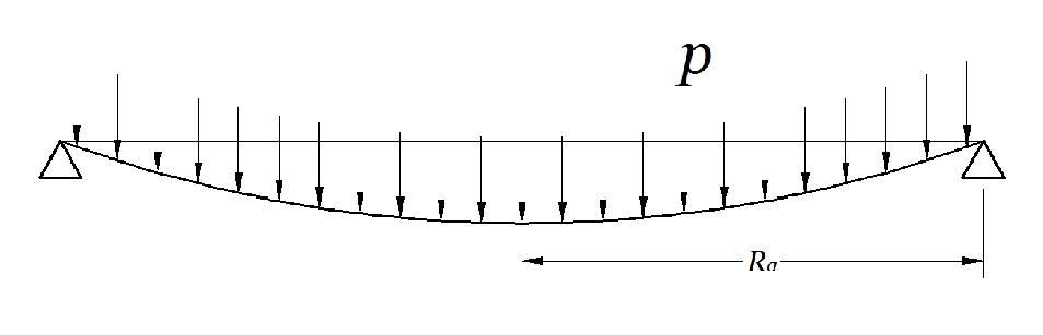
As shown in Fig. 1, four types of boundary conditions are considered:

  1. (a)

    Clamped: λ=0\lambda=0 and μ=2/(1−ν)\mu=2/(1-\nu);

  2. (b)

    Moveable clamped: λ=0\lambda=0 and μ=0\mu=0;

  3. (c)

    Simple support: λ=2/(1+ν)\lambda=2/(1+\nu) and μ=0\mu=0;

  4. (d)

    Simple hinged support: λ=2/(1+ν)\lambda=2/(1+\nu) and μ=2/(1−ν)\mu=2/(1-\nu);

Refer to caption
(a) Clamped
Refer to caption
(b) Moveable clamped
Refer to caption
(c) Simple support
Refer to caption
(d) Simple hinged support
Figure 1: Four types of boundary conditions

Over the past century, lots of analytic/numerical methods are proposed [8, 9, 10, 11, 12, 13, 14, 15] for the Von Kármán’s plate equations. Vincent [2] proposed a perturbation approach by using the load QQ as a small physical parameter, say,

φ⁡(y)=φ(V)​(y)=∑i=1+∞φi(V)​(y)​Q2​i−1,S⁡(y)=S(V)​(y)=∑i=1+∞Si(V)​(y)​Q2​i,\begin{split}\varphi(y)=\varphi^{(V)}(y)=\sum_{i=1}^{+\infty}\varphi_{i}^{(V)}(y)Q^{2i-1},\\ S(y)=S^{(V)}(y)=\sum_{i=1}^{+\infty}S_{i}^{(V)}(y)Q^{2i},\;\;\;\end{split} (8)

where φi(V)​(y)\varphi_{i}^{(V)}(y) and Si(V)​(y)S_{i}^{(V)}(y) are governed by

Q:{y2d2​φ1(V)​(y)d​y2=y2,y∈(0,1),φ1(V)(0)=0,φ1(V)(1)=λλ−1d​φ1(V)​(y)d​y|y=1;{Q:}\left\{\begin{split}{y^{2}\frac{d^{2}\varphi_{1}^{(V)}(y)}{dy^{2}}=}{~y^{2}}{,\;\;\;\;y\in(0,1),}~~~~~~~~~~~~~~~~~~~~~~~~~~~~~~~~\\ {\varphi_{1}^{(V)}(0)=0,\;\;\;\;\;\varphi_{1}^{(V)}(1)=\frac{\lambda}{\lambda-1}\frac{d\varphi_{1}^{(V)}(y)}{dy}\bigg|_{y=1};\;\;\;\;~~~~~~~~~~}\end{split}\right. (9)
Q2:{y2​d2​S1(V)​(y)d​y2=−12​(φ1(V)​(y))2,S1(V)(0)=0,S1(V)(1)=μμ−1d​S1(V)​(y)d​y|y=1;{Q^{2}:}\left\{\begin{split}{y^{2}\frac{d^{2}S_{1}^{(V)}(y)}{dy^{2}}=-\frac{1}{2}\left(\varphi_{1}^{(V)}(y)\right)^{2},}~~~~~~~~~~~~~~~~~~~~~~~~~~~~~\\ {S_{1}^{(V)}(0)=0,\;\;\;\;\;S_{1}^{(V)}(1)=\frac{\mu}{\mu-1}\frac{dS_{1}^{(V)}(y)}{dy}\bigg|_{y=1};~~~~~~~~~~}\end{split}\right. (10)

⋯⋯~~~~~\cdots\cdots

Q2​i+1:{y2​d2​φi+1(V)​(y)d​y2=∑j=1iφj(V)​(y)​Si−j+1(V)​(y),φi+1(V)(0)=0,φi+1(V)(1)=λλ−1d​φi+1(V)​(y)d​y|y=1;{Q^{2i+1}:}\left\{\begin{split}{y^{2}\frac{d^{2}\varphi_{i+1}^{(V)}(y)}{dy^{2}}=\sum_{j=1}^{i}\varphi_{j}^{(V)}(y)S_{i-j+1}^{(V)}(y),}~~~~~~~~~~~~~~~~~~~~~~~~~\\ {\varphi_{i+1}^{(V)}(0)=0,\;\;\;\;\varphi_{i+1}^{(V)}(1)=\frac{\lambda}{\lambda-1}\frac{d\varphi_{i+1}^{(V)}(y)}{dy}\bigg|_{y=1};~~~~~~~~~~~~~~}\end{split}\right. (11)
Q2​i+2:{y2d2​Si+1(V)​(y)d​y2=−12∑j=1i+1φj(V)(y)φi−j+2(V)(y),Si+1(V)(0)=0,Si+1(V)(1)=μμ−1d​Si+1(V)​(y)d​y|y=1.{Q^{2i+2}:}\left\{\begin{split}{y^{2}\frac{d^{2}S_{i+1}^{(V)}(y)}{dy^{2}}=-\frac{1}{2}\sum_{j=1}^{i+1}\varphi_{j}^{(V)}(y)\varphi_{i-j+2}^{(V)}(y),~~~~~~~~~~~~~~~~~~~~}\;\\ {S_{i+1}^{(V)}(0)=0,\;\;\;\;\;S_{i+1}^{(V)}(1)=\frac{\mu}{\mu-1}\frac{dS_{i+1}^{(V)}(y)}{dy}\bigg|_{y=1}.~~~~~~~~~~~~~~}\end{split}\right. (12)

In the case of circular plate with clamped boundary (λ=0\lambda=0, μ=20/7\mu=20/7), the Vincent’s perturbation solutions are:

φ1(V)​(y)\displaystyle{\varphi_{1}^{(V)}(y)} =\displaystyle= −y2+y22,\displaystyle{-\frac{y}{2}+\frac{y^{2}}{2},} (13)
S1(V)​(y)\displaystyle{S_{1}^{(V)}(y)} =\displaystyle= 41​y672−y216+y324−y496,\displaystyle{\frac{41y}{672}-\frac{y^{2}}{16}+\frac{y^{3}}{24}-\frac{y^{4}}{96},} (14)
φ2(V)​(y)\displaystyle{\varphi_{2}^{(V)}(y)} =\displaystyle= 659​y80640−41​y22688+83​y38064−5​y41152+y5768−y65760,\displaystyle{\frac{659y}{80640}-\frac{41y^{2}}{2688}+\frac{83y^{3}}{8064}-\frac{5y^{4}}{1152}+\frac{y^{5}}{768}-\frac{y^{6}}{5760},} (15)
S2(V)​(y)\displaystyle{S_{2}^{(V)}(y)} =\displaystyle= −2357​y1505280+659​y2322560−1889​y3967680+103​y496768−59​y5161280\displaystyle{-\frac{2357y}{1505280}+\frac{659y^{2}}{322560}-\frac{1889y^{3}}{967680}+\frac{103y^{4}}{96768}-\frac{59y^{5}}{161280}} (16)
+13​y6138240−17​y7967680+y8645120,\displaystyle{+\frac{13y^{6}}{138240}-\frac{17y^{7}}{967680}+\frac{y^{8}}{645120},}
⋯⋯\displaystyle\cdots\cdots

Unfortunately, Vincent’s perturbation method is valid only for rather small ratio of central deflection to plate thickness w⁡(0)/h<0.52w(0)/h<0.52 for a circular plate with clamped boundary [2]. Thereafter, extensive researches were done to find a better perturbation quantity. For instance, the central deflection and the average angular deflection were used by Chien [3], Chien and Yeh [16] and Hu [17] as perturbation quantity. It is found [18] that the central deflection is the best, which can give perturbation results convergent within w⁡(0)/h<2.44w(0)/h<2.44 for clamped boundary [3]. Expanding φ⁡(y)\varphi(y), S⁡(y)S(y) and QQ into power series of the central deflection W⁡(0)W(0), we have

{φ⁡(y)=φ(C)​(y)=∑m=1+∞φm(C)​(y)​W2​m−1​(0),S⁡(y)=S(C)​(y)=∑m=1+∞Sm(C)​(y)​W2​m​(0),Q=Q(C)=∑m=1+∞Qm(C)​W2​m−1​(0).\left\{\begin{split}\varphi(y)=\varphi^{(C)}(y)=\sum_{m=1}^{+\infty}\varphi_{m}^{(C)}(y)W^{2m-1}(0),\\ S(y)=S^{(C)}(y)=\sum_{m=1}^{+\infty}S_{m}^{(C)}(y)W^{2m}(0),~~\\ Q=Q^{(C)}=\sum_{m=1}^{+\infty}Q_{m}^{(C)}W^{2m-1}(0).~~~~~~~\end{split}\right. (17)

The procedures of Chien’s perturbation method [3, 5] are:

W(0):{y2d2​φ1(C)​(y)d​y2=Q1(C)y2,y∈(0,1),φ1(C)(0)=0,φ1(C)(1)=λλ−1d​φ1(C)​(y)d​y|y=1,−∫011ϵφ1(C)(ϵ)dϵ=1;{W(0):}\left\{\begin{split}{y^{2}\frac{d^{2}\varphi_{1}^{(C)}(y)}{dy^{2}}=Q_{1}^{(C)}y^{2},\;\;\;\;y\in(0,1),~~~~~~~~~~~~~~~~~~~~~}\\ {\varphi_{1}^{(C)}(0)=0,\;\;\;\;\varphi_{1}^{(C)}(1)=\frac{\lambda}{\lambda-1}\frac{d\varphi_{1}^{(C)}(y)}{dy}\bigg|_{y=1},~~~~~~~~}\\ {-\int_{0}^{1}\frac{1}{\epsilon}\varphi_{1}^{(C)}(\epsilon)d\epsilon=\textbf{1};}\qquad\qquad\qquad\qquad\qquad~~~~~~~~\end{split}\right. (18)
W2(0):{y2​d2​S1(C)​(y)d​y2=−12​(φ1(C)​(y))2,S1(C)(0)=0,S1(C)(1)=μμ−1d​S1(C)​(y)d​y|y=1;{W^{2}(0):}\left\{\begin{split}{y^{2}\frac{d^{2}S_{1}^{(C)}(y)}{dy^{2}}=-\frac{1}{2}\left(\varphi_{1}^{(C)}(y)\right)^{2},\;\;\;\;}~~~~~~~~~~~~~~~~~~~~~~~~\\ {S_{1}^{(C)}(0)=0,\;\;\;\;S_{1}^{(C)}(1)=\frac{\mu}{\mu-1}\frac{dS_{1}^{(C)}(y)}{dy}\bigg|_{y=1};~~~~~~~~~}\end{split}\right. (19)

⋯⋯~~~~~\cdots\cdots

W2​i+1(0):{y2​d2​φi+1(C)​(y)d​y2=∑j=1iφj(C)​(y)​Si−j+1(C)​(y)+Qi+1(C)​y2,φi+1(C)(0)=0,φi+1(C)(1)=λλ−1d​φi+1(C)​(y)d​y|y=1,−∫011ϵφi+1(C)(ϵ)dϵ=0;{W^{2i+1}(0):}\left\{\begin{split}{y^{2}\frac{d^{2}\varphi_{i+1}^{(C)}(y)}{dy^{2}}=\sum_{j=1}^{i}\varphi_{j}^{(C)}(y)S_{i-j+1}^{(C)}(y)+Q_{i+1}^{(C)}y^{2},}\;\;\;\;~~~~~~~\\ {\varphi_{i+1}^{(C)}(0)=0,\;\;\varphi_{i+1}^{(C)}(1)=\frac{\lambda}{\lambda-1}\frac{d\varphi_{i+1}^{(C)}(y)}{dy}\bigg|_{y=1},~~~~~~~~~~~~~}\\ {-\int_{0}^{1}\frac{1}{\epsilon}\varphi_{i+1}^{(C)}(\epsilon)d\epsilon=0;~~~~~~~~~~~~~~~~~~~~~~~~~~~~~~~~~~~~~~~~}\end{split}\right. (20)
W2​i+2(0):{y2d2​Si+1(C)​(y)d​y2=−12∑j=1i+1φj(C)(y)φi−j+2(C)(y),Si+1(C)(0)=0,Si+1(C)(1)=μμ−1d​Si+1(C)​(y)d​y|y=1;{W^{2i+2}(0):}\left\{\begin{split}{y^{2}\frac{d^{2}S_{i+1}^{(C)}(y)}{dy^{2}}=-\frac{1}{2}\sum_{j=1}^{i+1}\varphi_{j}^{(C)}(y)\varphi_{i-j+2}^{(C)}(y),}~~~~~~~~~~~~~~\;\\ {S_{i+1}^{(C)}(0)=0,\;\;\;\;S_{i+1}^{(C)}(1)=\frac{\mu}{\mu-1}\frac{dS_{i+1}^{(C)}(y)}{dy}\bigg|_{y=1};~~~~~~~~~~}\end{split}\right. (21)

In the case of clamped boundary (λ=0\lambda=0, μ=20/7\mu=20/7), we have the Chien’s perturbation solutions

φ1(C)​(y)\displaystyle{\varphi_{1}^{(C)}(y)} =\displaystyle= −2​y+2​y2,\displaystyle{-2y+2y^{2},} (22)
s1(C)​(y)\displaystyle{s_{1}^{(C)}(y)} =\displaystyle= 41​y42−y2+2​y33−y46,\displaystyle{\frac{41y}{42}-y^{2}+\frac{2y^{3}}{3}-\frac{y^{4}}{6},} (23)
φ2(C)​(y)\displaystyle{\varphi_{2}^{(C)}(y)} =\displaystyle= 233​y1890−2179​y23780+83​y3126−5​y418+y512−y690,\displaystyle{\frac{233y}{1890}-\frac{2179y^{2}}{3780}+\frac{83y^{3}}{126}-\frac{5y^{4}}{18}+\frac{y^{5}}{12}-\frac{y^{6}}{90},} (24)
s2(C)​(y)\displaystyle{s_{2}^{(C)}(y)} =\displaystyle= −211​y19845+233​y21890−529​y32268+667​y43240−59​y5630\displaystyle{-\frac{211y}{19845}+\frac{233y^{2}}{1890}-\frac{529y^{3}}{2268}+\frac{667y^{4}}{3240}-\frac{59y^{5}}{630}} (25)
+13​y6540−17​y73780+y82520,\displaystyle{+\frac{13y^{6}}{540}-\frac{17y^{7}}{3780}+\frac{y^{8}}{2520},}
⋯⋯\displaystyle\cdots\cdots

Unfortunately, as pointed out by Volmir [19], the deflection curve given by the Chien’s perturbation method [3] becomes concave at centre when the central deformation increases to a certain level, which is obviously in contradiction with physical phenomena.

In summary, for circular plate under uniform external pressure, the previous perturbation methods [2, 3] are valid only for the small physical parameters, i.e. corresponding to the weak nonlinearity.

In 19651965 a modified iteration method was proposed by Yeh and Liu [4], which inherits the merits of iteration technique and Chien’s perturbation method [3]. The procedures of the modified iteration method [4, 5] are as follows:

y2​d2​ψn​(y)d​y2\displaystyle y^{2}\frac{d^{2}\psi_{n}(y)}{dy^{2}} =\displaystyle= −12​ϑn2​(y),\displaystyle-\frac{1}{2}\vartheta_{n}^{2}(y), (26)
y2​d2​ϑn+1​(y)d​y2\displaystyle y^{2}\frac{d^{2}\vartheta_{n+1}(y)}{dy^{2}} =\displaystyle= ϑn​(y)​ψn​(y)+Qn​y2,\displaystyle\vartheta_{n}(y)\psi_{n}(y)+Q_{n}y^{2}, (27)

subject to the boundary conditions

ϑn+1​(0)=ψn​(0)=0,\vartheta_{n+1}(0)=\psi_{n}(0)=0, (28)
ϑn+1​(1)=λλ−1⋅d​ϑn+1​(y)d​y|y=1,ψn​(1)=μμ−1⋅d​ψn​(y)d​y|y=1,\vartheta_{n+1}(1)=\frac{\lambda}{\lambda-1}\cdot\frac{d\vartheta_{n+1}(y)}{dy}\bigg|_{y=1},\;\;\;\;\psi_{n}(1)=\frac{\mu}{\mu-1}\cdot\frac{d\psi_{n}(y)}{dy}\bigg|_{y=1}, (29)

with the restriction condition

W(0)=a=−∫011εϑn+1(ε)dεW(0)=a=-\int_{0}^{1}\frac{1}{\varepsilon}\vartheta_{n+1}(\varepsilon)d\varepsilon (30)

and the initial guess

ϑ1​(y)=−2​a2​λ+1​[(λ+1)​y−y2].\vartheta_{1}(y)=\frac{-2a}{2\lambda+1}[(\lambda+1)y-y^{2}]. (31)

However, Zhou [20] studied the relationship between Chien’s perturbation solutions [3] and the modified iterative solutions [4], but found that they have the same convergent region. The modified iterative method [4], therefore, is also only valid for a small central deflection, too. Therefore, iteration itself can not enlarge the convergence radius of perturbation series, although greatly boosts the computational efficiency.

Keller and Reiss [21] proposed the interpolation iterative method by introducing an interpolation parameter to the iteration procedure. Fortunately, the interpolation iterative method yields convergent solutions even for loads as large as Q=7000Q=7000. However, while all of the iterations can be obtained explicitly as polynomials, their degrees increase geometrically. Keller and Reiss [21], therefore, computed the iterations approximately by means of finite differences and gave numerical results. In 19881988, Zheng and Zhou [22] proved that the series solutions given by the interpolation iterative method are convergent for arbitrary values of load if proper interpolation iterative parameter is chosen [22].

In this paper, the same problem is solved by means of the homotopy analysis method (HAM) [23, 24, 25, 26], an analytic approximation technique proposed by Liao [23] for highly nonlinear problems. Unlike perturbation technique, the HAM is independent of any small/large physical parameters. Besides, it provides great freedom to choose equation-type and solution expression of the high-order approximation equations. Especially, the HAM also provides us a convenient way to guarantee the convergence of series solutions by means of introducing the so-called “convergence-control parameter" c0c_{0}. It should be emphasized that some mathematical theorems of convergence have been rigorously proved in the frame of the HAM [25]. For instance, it has been proved [25] that the power series given by the HAM

u⁡(t)=limm→+∞∑n=0mμ0m,n​(c0)​(−t)n,u(t)=\lim_{m\rightarrow+\infty}\sum_{n=0}^{m}\mu_{0}^{m,n}(c_{0})(-t)^{n}, (32)

where

μ0m,n​(c0)=(−c0)n​∑k=0m−n(n−1+kk)​(1+c0)k,\mu_{0}^{m,n}(c_{0})=(-c_{0})^{n}\sum_{k=0}^{m-n}\binom{n-1+k}{k}(1+c_{0})^{k}, (33)

converge to 1/(1+t)1/(1+t) in the intervals:

−1<t<−2c0−1,w​h​e​n​c0<0,-1<t<-\frac{2}{c_{0}}-1,\qquad when\;\;c_{0}<0, (34)

and

−2c0−1<t<−1,w​h​e​n​c0>0,-\frac{2}{c_{0}}-1<t<-1,\qquad when\;\;c_{0}>0, (35)

respectively. So, the power series (32) converges to 1/(1+t)1/(1+t) either in the interval (−1,+∞)(-1,+\infty) if c0<0c_{0}<0 impends 00, or in the interval (−∞,−1)(-\infty,-1) if c0>0c_{0}>0 tends to 00, respectively. In other words, the introduction of the convergence-control parameter c0c_{0} allows the power series (32) to converge to 1/(1+t)1/(1+t) in its entire definition domain. Note that the traditional power series (regarding tt as a small variable):

11+t∼1−t+t2−t3+t4−⋯\frac{1}{1+t}\sim 1-t+t^{2}-t^{3}+t^{4}-\cdots (36)

only converges in the interval (−1,1)(-1,1). Thus, the so-called “convergence-control parameter" c0c_{0} can indeed greatly enlarge the convergence interval of solution series. As a powerful technique to solve highly nonlinear equations, the HAM has been successfully employed to solve various types of nonlinear problems over the past two decades [27, 28, 29, 30, 31, 32, 33, 34, 35, 36]. Note that the Föppl-Von Kármán’s plate equations was solved by means of the HAM [37]. Especially, the HAM can bring us something completely new/different: the steady-state resonant waves were first predicted by the HAM in theory [38, 39, 40, 41] and then confirmed experimentally in a laboratory [40].

In this paper, Von Kármán’s plate equations in the differential form with clamped boundary are solved at first. By means of the normal HAM (without iteration), convergent results are obtained in the case of w⁡(0)/h=3.03w(0)/h=3.03, which is larger than the maximum convergent range (w⁡(0)/h<2.44w(0)/h<2.44) of the perturbation method [18]. Further, an iteration approach is proposed in the frame of the HAM to gain convergent solutions within a rather large ratio of w⁡(0)/h>20w(0)/h>20, corresponding to a case of rather high nonlinearity. Our HAM approximations agree well with those given by the interpolation iterative method [5]. Furthermore, analytic approximations for other three boundaries (moveable clamped, simple support and simple hinged support) are also presented in a similar way. In addition, we prove that the previous perturbation methods (including Vincent’s [2] and Chien’s [3] perturbation methods) and the modified iteration method [4] are only special cases of the HAM.

2 Analytic approach based on the HAM

Like Zheng [5], we express φ⁡(y)\varphi(y) and S⁡(y)S(y) in power series

φ⁡(y)=∑m=1+∞am⋅ym,S⁡(y)=∑m=1+∞bm⋅ym,\varphi(y)=\sum_{m=1}^{+\infty}a_{m}\cdot y^{m},\;\;\;\;S(y)=\sum_{m=1}^{+\infty}b_{m}\cdot y^{m}, (37)

where ama_{m} and bmb_{m} are constant coefficients to be determined. This provides us the so-called “solution expression” of φ⁡(y)\varphi(y) and S⁡(y)S(y) in the frame of the HAM. Writing

W⁡(0)=a,W(0)=a, (38)

we have due to Eq. (7) an algebraic equation:

∫011ε​φ​(ε)​𝑑ε=−a.\int_{0}^{1}\frac{1}{\varepsilon}\varphi(\varepsilon)d\varepsilon=-a. (39)

Let φ0​(y)\varphi_{0}(y) and S0​(y)S_{0}(y) denote the initial guesses of φ⁡(y)\varphi(y) and S⁡(y)S(y), respectively, which satisfy the boundary conditions (3), (4) and (39). Moreover, let ℒ\mathcal{L} denote an auxiliary linear operator with property ℒ⁡[0]=0{\cal L}[0]=0, H1​(y)H_{1}(y) and H2​(y)H_{2}(y) the auxiliary functions, c0c_{0} a non-zero auxiliary parameter, called the convergence-control parameter, and q∈[0,1]q\in[0,1] the embedding parameter, respectively. We construct a family of differential equations in q∈[0,1]q\in[0,1]:

(1−q)​ℒ​[Φ⁡(y,q)−φ0​(y)]\displaystyle(1-q)\mathcal{L}\big[\Phi(y;q)-\varphi_{0}(y)\big] (40)
=\displaystyle= c0​q​H1​(y)​[y2​∂2Φ⁡(y,q)∂y2−Φ⁡(y,q)​Ξ​(y,q)−Θ⁡(q)​y2],\displaystyle c_{0}qH_{1}(y)\bigg[y^{2}\frac{\partial^{2}\Phi(y;q)}{\partial y^{2}}-\Phi(y;q)\Xi(y;q)-\Theta(q)y^{2}\bigg],
(1−q)​ℒ​[Ξ⁡(y,q)−S0​(y)]\displaystyle(1-q)\mathcal{L}\big[\Xi(y;q)-S_{0}(y)\big]
=\displaystyle= c0​q​H2​(y)​[y2​∂2Ξ⁡(y,q)∂y2+12​Φ2​(y,q)],\displaystyle c_{0}qH_{2}(y)\bigg[y^{2}\frac{\partial^{2}\Xi(y;q)}{\partial y^{2}}+\frac{1}{2}\Phi^{2}(y;q)\bigg], (41)

subject to the boundary conditions

Φ⁡(0,q)=Ξ⁡(0,q)=0,\Phi(0;q)=\Xi(0;q)=0, (42)
Φ⁡(1,q)=λλ−1⋅∂Φ⁡(y,q)∂y|y=1,Ξ⁡(1,q)=μμ−1⋅∂Ξ⁡(y,q)∂y|y=1,\Phi(1;q)=\frac{\lambda}{\lambda-1}\cdot\frac{\partial\Phi(y;q)}{\partial y}\bigg|_{y=1},\;\;\;\;\Xi(1;q)=\frac{\mu}{\mu-1}\cdot\frac{\partial\Xi(y;q)}{\partial y}\bigg|_{y=1}, (43)

with the restriction condition

∫011ε​Φ​(ε,q)​𝑑ε=−a.\int_{0}^{1}\frac{1}{\varepsilon}\Phi(\varepsilon;q)d\varepsilon=-a. (44)

Note that Φ⁡(y,q),Ξ⁡(y,q)\Phi(y;q),\Xi(y;q) and Θ⁡(q)\Theta(q) correspond to the unknown φ⁡(y),S⁡(y)\varphi(y),S(y) and QQ, respectively, as mentioned below.

Note that QQ is unknown for a given value of W⁡(0)=aW(0)=a. Expand Θ⁡(q)\Theta(q) in a power series

Θ⁡(q)=Q0+∑m=1+∞Qm​qm,\Theta(q)=Q_{0}+\sum_{m=1}^{+\infty}Q_{m}\;q^{m}, (45)

where

Qm=𝒟m​[Θ⁡(q)],Q_{m}={\cal D}_{m}[\Theta(q)], (46)

is determined later, in which

𝒟m​[f]=1m!​∂mf∂qm|q=0{\cal D}_{m}[f]=\frac{1}{m!}\frac{\partial^{m}f}{\partial q^{m}}\bigg|_{q=0} (47)

is called the mmth-order homotopy-derivative of ff.

When q=0q=0, due to the property ℒ⁡(0)=0\mathcal{L}(0)=0, Eqs. (40)-(44) have the solution

Φ⁡(y,0)=φ0​(y),Ξ⁡(y,0)=S0​(y).\Phi(y;0)=\varphi_{0}(y),\;\;\;\;\;\;\Xi(y;0)=S_{0}(y). (48)

When q=1q=1, Eqs. (40)-(44) are equivalent to the original equations (1)-(4) and (39), provided

Φ⁡(y,1)=φ⁡(y),Ξ⁡(y,1)=S⁡(y),Θ⁡(1)=Q.\Phi(y;1)=\varphi(y),\;\;\;\;\Xi(y;1)=S(y),\;\;\;\;\Theta(1)=Q. (49)

Therefore, as the embedding parameter qq increases from 00 to 11, Φ⁡(y,q)\Phi(y;q) varies (or deforms) continuously from the initial guess φ0​(y)\varphi_{0}(y) to φ⁡(y)\varphi(y), so do Ξ⁡(y,q)\Xi(y;q) from the initial guess S0​(y)S_{0}(y) to S⁡(y)S(y), and Θ⁡(q)\Theta(q) from Q0Q_{0} to QQ, respectively. So, we call Eqs. (40)-(44) the zeroth-order deformation equation. Note that Q0Q_{0} is an unknown constant at present, which will be determined later.

Using (48), we have the power series

Φ⁡(y,q)=φ0​(y)+∑m=1+∞φm​(y)​qm,Ξ⁡(y,q)=S0​(y)+∑m=1+∞Sm​(y)​qm,\displaystyle\Phi(y;q)=\varphi_{0}(y)+\sum_{m=1}^{+\infty}\varphi_{m}(y)\;q^{m},\;\;\;\Xi(y;q)=S_{0}(y)+\sum_{m=1}^{+\infty}S_{m}(y)\;q^{m}, (50)

in which

φm​(y)=𝒟m​[Φ⁡(y,q)],Sm​(y)=𝒟m​[Ξ⁡(y,q)],\varphi_{m}(y)={\cal D}_{m}[\Phi(y;q)],\;\;\;\;\;\;S_{m}(y)={\cal D}_{m}[\Xi(y;q)], (51)

where 𝒟m{\cal D}_{m} is defined by (47).

It is well-known that convergence radius of a power series is finite in general. Fortunately, in the frame of the HAM, we have great freedom to choose the auxiliary linear operator ℒ\cal L and especially the so-called convergence-control parameter c0c_{0}. Assume that all of them are properly chosen so that the power series (45) and (50) are convergent at q=1q=1. Then, according to (49), we have the so-called homotopy-series solution

φ⁡(y)=∑m=0+∞φm​(y),S⁡(y)=∑m=0+∞Sm​(y),Q=∑m=0+∞Qm.\varphi(y)=\sum_{m=0}^{+\infty}\varphi_{m}(y),\;\;\;\;S(y)=\sum_{m=0}^{+\infty}S_{m}(y),\;\;\;\;Q=\sum_{m=0}^{+\infty}Q_{m}. (52)

The governing equations and boundary conditions of φm​(y)\varphi_{m}(y), Sm​(y)S_{m}(y) and Qm−1Q_{m-1} are obtained in the following way. Substituting (45) and (50) into the zeroth-order deformation equations (40)-(44) and then equating the like-power of qq, we have the so-called mmth-order deformation equations

ℒ⁡[φm​(y)−χm​φm−1​(y)]=c0​H1​(y)​δ1,m−1​(y),\displaystyle\mathcal{L}[\varphi_{m}(y)-\chi_{m}\varphi_{m-1}(y)]=c_{0}H_{1}(y)\delta_{1,m-1}(y), (53)
ℒ⁡[Sm​(y)−χm​Sm−1​(y)]=c0​H2​(y)​δ2,m−1​(y),\displaystyle\mathcal{L}[S_{m}(y)-\chi_{m}S_{m-1}(y)]=c_{0}H_{2}(y)\delta_{2,m-1}(y), (54)

subject to the boundary conditions

φm​(0)=Sm​(0)=0,\varphi_{m}(0)=S_{m}(0)=0, (55)
φm​(1)=λλ−1⋅d​φm​(y)d​y|y=1,Sm​(1)=μμ−1⋅d​Sm​(y)d​y|y=1,\varphi_{m}(1)=\frac{\lambda}{\lambda-1}\cdot\frac{d\varphi_{m}(y)}{dy}\bigg|_{y=1},\;\;\;\;S_{m}(1)=\frac{\mu}{\mu-1}\cdot\frac{dS_{m}(y)}{dy}\bigg|_{y=1}, (56)

with the restriction condition

∫011ε⋅φm​(ε)​𝑑ε=0,\int_{0}^{1}\frac{1}{\varepsilon}\cdot\varphi_{m}(\varepsilon)d\varepsilon=0, (57)

where

χm={0when m≤1,1when m>1,\chi_{m}=\left\{\begin{array}[]{cc}{0}&\mbox{when $m\leq 1$},\\ {1}&\mbox{when $m>1$,}\end{array}\right. (58)

and

δ1,m−1​(y)\displaystyle\delta_{1,m-1}(y) =\displaystyle= y2​d2​φm−1​(y)d​y2−∑k=0m−1φk​(y)​Sm−1−k​(y)−Qm−1​y2,\displaystyle y^{2}\frac{d^{2}\varphi_{m-1}(y)}{dy^{2}}-\sum_{k=0}^{m-1}\varphi_{k}(y)S_{m-1-k}(y)-Q_{m-1}y^{2}, (59)
δ2,m−1​(y)\displaystyle\delta_{2,m-1}(y) =\displaystyle= y2​d2​Sm−1​(y)d​y2+12​∑k=0m−1φk​(y)​φm−1−k​(y).\displaystyle y^{2}\frac{d^{2}S_{m-1}(y)}{dy^{2}}+\frac{1}{2}\sum_{k=0}^{m-1}\varphi_{k}(y)\varphi_{m-1-k}(y). (60)

According to the solution expression (37), we choose

φ0​(y)=−2​a2​λ+1​[(λ+1)​y−y2],S0​(y)=(μ+1)​y−y2\varphi_{0}(y)=\frac{-2a}{2\lambda+1}[(\lambda+1)y-y^{2}],\;\;\;\;\;\;\;\;S_{0}(y)=(\mu+1)y-y^{2} (61)

as the initial guesses of φ⁡(y)\varphi(y) and S⁡(y)S(y), and such an auxiliary linear operator

ℒ⁡[u⁡(y)]=d2​u​(y)d​y2.\mathcal{L}[u(y)]=\frac{d^{2}u(y)}{dy^{2}}. (62)

Note that the initial guesses (61) satisfy all boundary conditions. Similarly, according to the solution expression (37), the auxiliary functions H1​(y)H_{1}(y) and H2​(y)H_{2}(y) should be properly chosen so as to make sure that the right-hand sides of the high-order deformation equations (53) and (54) are in the forms

c0​H1​(y)​δ1,m−1​(y)\displaystyle c_{0}H_{1}(y)\delta_{1,m-1}(y) =\displaystyle= ∑k=0d1,k​yk,\displaystyle\sum_{k=0}d_{1,k}\;y^{k}, (63)
c0​H2​(y)​δ2,m−1​(y)\displaystyle c_{0}H_{2}(y)\delta_{2,m-1}(y) =\displaystyle= ∑k=0d2,k​yk,\displaystyle\sum_{k=0}d_{2,k}\;y^{k}, (64)

where d1,kd_{1,k} and d2,kd_{2,k} are constants. The auxiliary function H1​(y)H_{1}(y) and H2​(y)H_{2}(y), therefore, must be in the form

H1​(y)=H2​(y)=1y2.H_{1}(y)=H_{2}(y)=\frac{1}{y^{2}}. (65)

Then, we have the general solutions of the high-order deformation equation (53) and (54):

φm​(y)=χm​φm−1​(y)+c0​∫0y∫0ηδ1,m−1​(τ)τ2​𝑑τ​𝑑η+D1,m​y+D2,m,\varphi_{m}(y)=\chi_{m}\varphi_{m-1}(y)+c_{0}\int_{0}^{y}\int_{0}^{\eta}\frac{\delta_{1,m-1}(\tau)}{\tau^{2}}d\tau d\eta+D_{1,m}y+D_{2,m}, (66)
Sm​(y)=χm​Sm−1​(y)+c0​∫0y∫0ηδ2,m−1​(τ)τ2​𝑑τ​𝑑η+D3,m​y+D4,m,S_{m}(y)=\chi_{m}S_{m-1}(y)+c_{0}\int_{0}^{y}\int_{0}^{\eta}\frac{\delta_{2,m-1}(\tau)}{\tau^{2}}d\tau d\eta+D_{3,m}y+D_{4,m}, (67)

where D1,mD_{1,m}, D2,mD_{2,m}, D3,mD_{3,m}, D4,mD_{4,m} are determined by four linear boundary conditions (55) and (56), and the unknown Qm−1Q_{m-1} is determined by the restriction condition (57). In this way, φm​(y)\varphi_{m}(y) , Sm​(y)S_{m}(y) and Qm−1Q_{m-1} of Eqs. (53) and (54) can be obtained step by step, starting from m=1m=1. Then, we have the MMth-order homotopy-approximation of φ⁡(y)\varphi(y), S⁡(y)S(y) and QQ:

φ~​(y)=∑m=0Mφm​(y),S~​(y)=∑m=0MSm​(y),Q~=∑m=0MQm.\tilde{\varphi}(y)=\sum_{m=0}^{M}\varphi_{m}(y),\;\;\;\;\tilde{S}(y)=\sum_{m=0}^{M}S_{m}(y),\;\;\;\;\tilde{Q}=\sum_{m=0}^{M}Q_{m}. (68)

Define the squared residual error

ℰ=∫01{(𝒩1​[φ~​(y),S~​(y),y])2+(𝒩2​[φ~​(y),S~​(y),y])2}​𝑑y,{\cal E}=\int_{0}^{1}\left\{\bigg({\cal N}_{1}\left[\tilde{\varphi}(y),\tilde{S}(y),y\right]\bigg)^{2}+\bigg({\cal N}_{2}\left[\tilde{\varphi}(y),\tilde{S}(y),y\right]\bigg)^{2}\right\}dy, (69)

where the nonlinear operators defined by 𝒩1{\cal N}_{1} and 𝒩2{\cal N}_{2} are related to the original equations (1) and (2). Obviouly, the smaller the ℰ\cal E, the more accurate the HAM approximation. According to Liao [24, 25], the optimal value of the convergence-control parameter c0c_{0} is determined by the minimum of ℰ\cal E. It was proved [24, 25] in general cases that the homotopy-series converge to solutions of original equations as long as all squared residual errors tend to zero. So, it is enough to check the squared residual error (69) only.

According to Liao [24], convergence of the homotopy-series solutions can be greatly accelerated by means of iteration technique, which uses the MMth-order homotopy-approximation (67) as the new initial guesses φ0​(y)\varphi_{0}(y) and S0​(y)S_{0}(y) for the next iteration. This provides us the MMth-order iteration of the HAM. In the iteration process of the HAM, the right-hand side of Eqs. (53) and (54) are truncated to yNy^{N}, say,

c0​H1​(y)⋅δ1,m​(y)≈∑k=0NEm,k⋅yk,c0​H2​(y)⋅δ2,m​(y)≈∑k=0NFm,k⋅yk,c_{0}H_{1}(y)\cdot\delta_{1,m}(y)\approx\sum_{k=0}^{N}E_{m,k}\cdot y^{k},\;\;\;\;c_{0}H_{2}(y)\cdot\delta_{2,m}(y)\approx\sum_{k=0}^{N}F_{m,k}\cdot y^{k}, (70)

where Em,kE_{m,k} and Fm,kF_{m,k} are constants and NN is called the truncation order.

3 Result analysis

Without loss of generality, the Poisson’s ratio ν\nu is taken to be 0.30.3 in all cases considered in this paper.

3.1 The HAM-based approach without iteration

Without loss of generality, let us consider the clamped boundary in the case of a=5a=5, equivalent to w⁡(0)/h=3.03w(0)/h=3.03. At the beginning, the so-called convergence-control parameter c0c_{0} is unknown. Its optimal value (i.e. -0.28 in this case) is determined by the minimum of the squared residual error defined by (69). According to Table 1, the squared residual error decreases to 4.9×10−124.9\times 10^{-12} by means of c0=−0.28c_{0}=-0.28. So, unlike perturbation method that is valid only for w⁡(0)/h<2.44w(0)/h<2.44 in the same case [18], we gain convergent result by means of the HAM. This is mainly because the so-called convergence-control parameter in the frame of the HAM provides us a convenient way to guarantee the convergence of solution series.

Table 1: The approximations of QQ, the squared residual errors E​r​rErr and the used CPU time in the case of a=5a=5 with the clamped boundary by means of the HAM (without iteration) using c0=−0.28c_{0}=-0.28.
 
mm, order of approx. ℰ\cal E      QQ CPU time (seconds)
20 6.4×10−26.4\times 10^{-2} 131.7 6
40 5.8×10−45.8\times 10^{-4} 132.1 35
60 9.3×10−69.3\times 10^{-6} 132.1 106
80 2.0×10−72.0\times 10^{-7} 132.2 243
100 5.1×10−95.1\times 10^{-9} 132.2 465
120 1.5×10−101.5\times 10^{-10} 132.2 782
140 4.9×10−124.9\times 10^{-12} 132.2 1205
 
Table 2: The approximations of QQ, the squared residual errors ℰ\cal E and the used CPU time versus iteration times in the case of a=5a=5 with the clamped boundary, given by the1st-order HAM iteration approach using c0=−0.55c_{0}=-0.55 with the truncation order N=100N=100.
 
mm, times of iteration ℰ\cal E     QQ CPU time (seconds)
10 4.5×10−34.5\times 10^{-3} 132.2 5
20 4.8×10−114.8\times 10^{-11} 132.2 12
30 1.3×10−181.3\times 10^{-18} 132.2 18
40 1.7×10−241.7\times 10^{-24} 132.2 25
 

Given a value of aa, the optimal value of c0c_{0} for the Von Kármán’s plate equations with clamped boundary can be obtained in a similarly, which can be expressed by such an empirical formula

c0=−5050+0.45⋅a72(0≤a≤5).c_{0}=-\frac{50}{50+0.45\cdot a^{\frac{7}{2}}}\;\;\;\;\;(0\leq a\leq 5). (71)

Note that, like perturbation approximations, all of these homotopy-approximations of φ⁡(y)\varphi(y) and S⁡(y)S(y) are expressed in polynomial for a given value of aa.

In Appendix A, we prove that the previous perturbation methods for an arbitrary perturbation quantity (including the Vincent’s [2] and Chien’s [3] methods) are only the special cases of the HAM when c0=−1c_{0}=-1. This also explains why the HAM can give convergent results for larger w⁡(0)/hw(0)/h: the convergence-control parameter c0c_{0} plays an important role in the guarantee of convergence of solution series.

3.2 Convergence acceleration by means of iteration

Iteration can be naturally introduced into the frame of the HAM to greatly accelerate the convergence, as illustrated by Liao [24, 25]. Without loss of generality, let us first consider here the same case of a=5a=5 with the clamped boundary. It is found that the squared residual error arrives its minimum at c0≈−0.55c_{0}\approx-0.55 by means of the HAM-based 1st-order iteration approach with the truncation order N=100N=100. As shown in Table 2, the squared residual error quickly decreases to 1.7×10−241.7\times 10^{-24} in only 2525 seconds, which is about 100100 times faster than the HAM approach without iteration. Thus, from the viewpoint of computational efficiency, the iteration HAM approach is used below in the subsequent part of this paper.

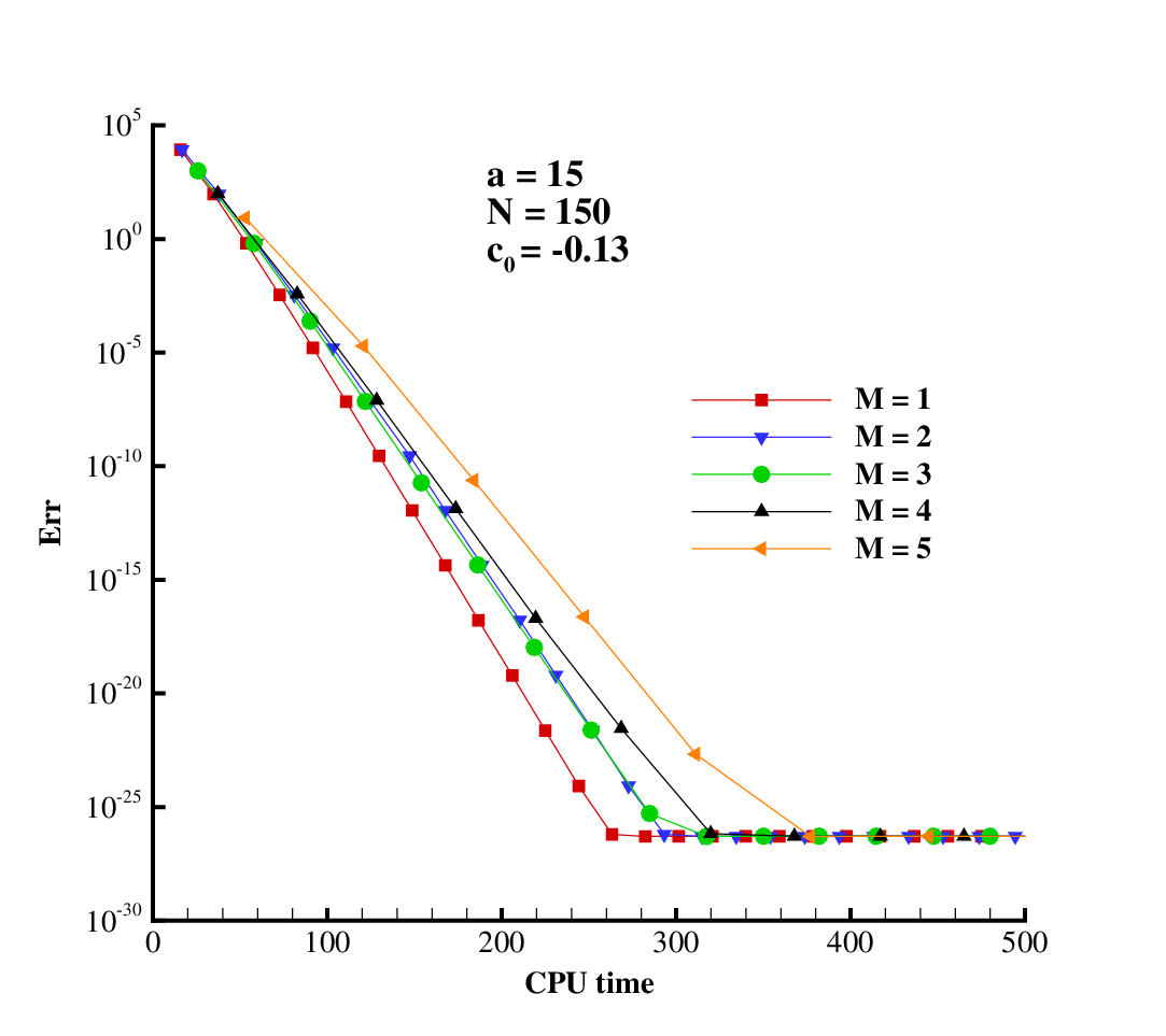
The HAM iteration approach contains two parameters, the iteration order MM and the truncation order NN. Without loss of generality, let us further consider the case of a=15a=15, corresponding to a higher nonlinearity. As shown in Fig. 2, the squared residual errors decrease to the level of 10−2610^{-26} with different iteration order MM: the higher-order iteration need less iteration times, but more CPU times. Thus, from the computational efficiency, the first-order HAM iteration approach is suggested.

Refer to caption Refer to caption
Figure 2: The squared residual error versus the times of iteration and the CPU times in the case of a=15a=15 with clamped boundary, given by the HAM iteration approach using c0=−0.13c_{0}=-0.13 with the truncation order N=150N=150 and different order MM of iteration approach. Square: 1st-order; Triangle down: 2nd-order; Circle: 3rd-order; Triangle up: 4th-order; Triangle left: 5th-order.

In addition, it is found that the iteration converges with high accuracy when NN is large enough, but larger NN also corresponds to a slower convergence. Obviously, as the load increases, i.e. aa enlarges, the nonlinearity becomes stronger, so that larger NN is necessary. It is found that, in the frame of 1st-order HAM iteration approach, the following empirical formula for the truncation order is good enough for all cases in this paper:

N=M​a​x​{100,γ⋅a},N=Max\left\{100,\gamma\cdot a\right\}, (72)

where γ\gamma is dependent upon the type of boundary:

γ={10,c​l​a​m​p​e​d​b​o​u​n​d​a​r​y;13,m​o​v​e​a​b​l​e​c​l​a​m​p​e​d​b​o​u​n​d​a​r​y;7,s​i​m​p​l​e​s​u​p​p​o​r​t​b​o​u​n​d​a​r​y;5,s​i​m​p​l​e​h​i​n​g​e​d​s​u​p​p​o​r​t​b​o​u​n​d​a​r​y.\gamma=\left\{\begin{array}[]{llllll}10,~~~~~clamped~boundary;\\ 13,~~~~~moveable~clamped~boundary;\\ ~7,~~~~~simple~support~boundary;\\ ~5,~~~~~simple~hinged~support~boundary.\end{array}\right.
Table 3: The homotopy-approximation of the load QQ versus aa for clamped boundary, given by the HAM-based 1st-order iteration approach with the truncation order NN given by (72) and the optimal convergence-control parameter c0c_{0} given by (73).
 
aa      c0c_{0}     NN QQ
5 -0.51 100 132.2
10 -0.21 100 957.7
15 -0.10 150 3152.1
20 -0.06 200 7386.9
25 -0.04 250 14334.1
30 -0.03 300 24665.7
35 -0.02 350 39053.6
 

As shown in Table 3, by means of the 1st-order HAM iteration approach, the convergent results in polynomials are obtained by means of the optimal convergence-control parameter with the empirical formula

c0=−2626+a2(0≤a≤35)c_{0}=-\frac{26}{26+a^{2}}\;\;\;\;\;(0\leq a\leq 35) (73)

within a≤35a\leq 35, which is large enough for practice, since a=35a=35 corresponds to w⁡(0)/h=21.2w(0)/h=21.2

As shown in Fig. 3, Chien’s perturbation method [3] is valid only in the region of w⁡(0)/h<2.44w(0)/h<2.44, and becomes worser and worser for larger w⁡(0)/hw(0)/h. In addition, our HAM results agree quite well with those given by Zheng [5] using the interpolation iterative method, but converge in larger region. The obtained deflections under different loads are depicted in Fig. 4.

In Appendix B, we prove that the modified iteration method [4] are only a special cases of the HAM when c0=−1c_{0}=-1. This reveals why the modified iteration method [4] is valid for weak nonlinearity and besides shows the importance of the convergence-control parameter c0c_{0} in the frame of the HAM. In fact, it is the convergence-control parameter c0c_{0} that differs the HAM from all other analytic approximations [24, 25].

Refer to caption Refer to caption
Figure 3: Comparison of the results given by the HAM-based 1st-order iteration approach and other methods for clamped boundary. Solid line: results given by the HAM; Symbols: results given by Chien’s perturbation method [3] (left) and by Zheng [5] using the interpolation iterative method (right).
Refer to caption
Figure 4: The deflections of a thin circular plate with clamped boundary given by the HAM-based 1st-order iteration approach in the case of a=5,15,25,35a=5,15,25,35. Solid line: p​Ra4/E​h4=117.2pR_{a}^{4}/Eh^{4}=117.2; Dash-double-dotted line: p​Ra4/E​h4=2795.2pR_{a}^{4}/Eh^{4}=2795.2; Dash-dotted line: p​Ra4/E​h4=12711.2pR_{a}^{4}/Eh^{4}=12711.2; Dashed line: p​Ra4/E​h4=34632.0pR_{a}^{4}/Eh^{4}=34632.0.

Similarly, by means of the 1st-order HAM iteration approach, the convergent results for moveable clamped boundary are obtained by means of the optimal convergence-control parameter with the empirical formula

c0=−3939+a2c_{0}=-\frac{39}{39+a^{2}} (74)

within the range of a≤35a\leq 35, as shown in Table 4.

For simple support boundary, the convergent results are obtained by means of the optimal convergence-control parameter with the empirical formula

c0=−8080+a2c_{0}=-\frac{80}{80+a^{2}} (75)

within the range of 0≤a≤500\leq a\leq 50, as shown in Table 5. For a circular plate with the boundary of simple hinged support, the convergent results are obtained by means of the optimal convergence-control parameter with the empirical formula

c0=−4040+a52c_{0}=-\frac{40}{40+a^{\frac{5}{2}}} (76)

within the range of 0≤a≤500\leq a\leq 50, as shown in Table 6.

Table 4: The convergent homotopy-approximation of the load QQ in case of different values of aa for a circular plate with moveable clamped boundary, given by the HAM-based 1st-order iteration approach using the truncation order NN given by (72) and the optimal convergence-control parameter c0c_{0} given by (74).
 
aa      c0c_{0}     NN QQ
5 -0.61 100 49.3
10 -0.28 130 240.1
15 -0.15 195 657.7
20 -0.09 260 1372.5
25 -0.06 325 2450.9
30 -0.04 390 3956.8
35 -0.03 455 5952.2
 
Table 5: The convergent homotopy-approximation of the load QQ in case of different values of aa for a circular plate with the simple support boundary, given by the HAM-based 1st-order iteration approach with the truncation order NN given by (72) and the optimal convergence-control parameter c0c_{0} given by (75).
 
aa      c0c_{0}     NN QQ
10 -0.44 100 107.8
20 -0.17 140 737.4
30 -0.08 210 2304.8
40 -0.05 280 5199.8
50 -0.03 350 9799.3
 
Table 6: The convergent homotopy-approximation of the load QQ in case of different values of aa for a circular plate with the boundary of simple hinged support given by the HAM-based 1st-order iteration approach with the truncation order NN given by (72) and the optimal convergence-control parameter c0c_{0} given by (76).
 
aa      c0c_{0}     NN QQ
10 -0.112 100 890.0
20 -0.021 100 7152.3
30 -0.008 150 24166.4
40 -0.004 200 57308.7
50 -0.002 250 111955.3
 

4 Conclusions

In this paper, the homotopy analysis method (HAM) is applied to the large deflection of a circular thin plate under uniform external pressure. By means of choosing a proper value of the so-called convergence-control parameter c0c_{0} given by the empirical formulas (73), (74), (75) and (76), convergent results are successfully obtained even in the case of w⁡(0)/h>20w(0)/h>20 for four types of boundary conditions. Besides, it is found that iteration can greatly accelerate the convergence of solutions. In addition, we reveal that the previous perturbation methods for an arbitrary perturbation quantity (including the Vincent’s [2] and Chien’s [3] methods) and the modified iteration method [4] are only the special cases of the HAM†† † Even the interpolation iterative method [21] is also a special case of the HAM. Limited to the length of the paper, we will give the proof somewhere else when c0=−1c_{0}=-1. This reveals the reason why the previous perturbation techniques [2, 3] and the modified iteration method [4] are only valid for small physical parameters, corresponding to weak nonlinearity. This work shows once again that the convergence-control parameter c0c_{0} indeed plays a very important role in the frame of the HAM: it differs the HAM from all other analytic approximation methods.

This paper demonstrates the validity of the HAM for the Von Kármán plate equations, and also clearly shows the superiority of the HAM over perturbation methods. Without doubt, the HAM can be further applied to solve some challenging problems with high nonlinearity in solid mechanics.

Acknowledgment

This work is partly supported by National Natural Science Foundation of China (Approval No. 11272209 and 11432009) and State Key Laboratory of Ocean Engineering (Approval No. GKZD010063).

Appendix A. Relations between the perturbation methods and the HAM approach

Here we prove that the perturbation methods for an arbitrary perturbation quantity (including Vincent’s [2] and Chien’s [3] perturbation methods) are special cases of the HAM approach when c0=−1c_{0}=-1.

In general, the perturbation solutions can be expressed as:

uP​(y)=u0P​(y)+u1P​(y)​ε+u2P​(y)​ε2+⋯,{u^{P}(y)=u^{P}_{0}(y)+u^{P}_{1}(y)\varepsilon+u^{P}_{2}(y)\varepsilon^{2}+\cdot\cdot\cdot,}

where ε\varepsilon is a physical parameter. The HAM-series solutions are expressed by

uH​(y,c0)=u0H​(y,c0)+u1H​(y,c0)+u2H​(y,c0)+⋯.{u^{H}(y;c_{0})=u^{H}_{0}(y;c_{0})+u^{H}_{1}(y;c_{0})+u^{H}_{2}(y;c_{0})+\cdot\cdot\cdot.}

Obviously, if uiP​(y)​εiu^{P}_{i}(y)\varepsilon^{i} = uiH​(y,−1)u^{H}_{i}(y;-1), then uP​(y)u^{P}(y) is exactly the same as uH​(y,−1)u^{H}(y;-1), say, the perturbation method is a special case of the HAM when c0=−1c_{0}=-1.

First, we describe the perturbation methods for a circular plate under uniform pressure in a general way. Let ζ\zeta denote a perturbation quantity and write the perturbation series

{φ(P)(y)=∑i=1+∞φi(P)(y)ζ2​i−1,S(P)(y)=∑i=1+∞Si(P)(y)ζ2​i,Q(P)=∑i=1+∞Qi(P)ζ2​i−1,W(P)(0)=∑i=1+∞Wi(P)(0)ζ2​i−1.\left\{\begin{split}\varphi^{(P)}(y)=\sum_{i=1}^{+\infty}\varphi_{i}^{(P)}(y)\zeta^{2i-1},\;\;\;S^{(P)}(y)=\sum_{i=1}^{+\infty}S_{i}^{(P)}(y)\zeta^{2i},\;\;\;\;\\ \;\;\;\;\;\;Q^{(P)}=\sum_{i=1}^{+\infty}Q_{i}^{(P)}\zeta^{2i-1},\;\;\;\;\;W^{(P)}(0)=\sum_{i=1}^{+\infty}W_{i}^{(P)}(0)\zeta^{2i-1}.\end{split}\right. (A-1)

Define

S0(P)​(y)=0.S_{0}^{(P)}(y)=0.

Substituting (A-1) into Eqs. (1)-(4) and (7), and equating the like-power of ζ\zeta, we have the governing equations

y2​d2​φm(P)​(y)d​y2\displaystyle y^{2}\frac{d^{2}\varphi_{m}^{(P)}(y)}{dy^{2}} =\displaystyle= ∑i=1mφi(P)​(y)​Sm−i(P)​(y)+Qm(P)⋅y2,\displaystyle\sum_{i=1}^{m}\varphi_{i}^{(P)}(y)S_{m-i}^{(P)}(y)+Q_{m}^{(P)}\cdot y^{2}, (A-2)
y2​d2​Sm(P)​(y)d​y2\displaystyle y^{2}\frac{d^{2}S_{m}^{(P)}(y)}{dy^{2}} =\displaystyle= −12∑i=1mφi(P)(y)φm+1−i(P)(y),\displaystyle-\frac{1}{2}\sum_{i=1}^{m}\varphi_{i}^{(P)}(y)\varphi_{m+1-i}^{(P)}(y), (A-3)

subject to the boundary conditions

φm(P)​(0)=Sm(P)​(0)=0,\varphi_{m}^{(P)}(0)=S_{m}^{(P)}(0)=0, (A-4)
φm(P)​(1)=λλ−1⋅d​φm(P)​(y)d​y|y=1,Sm(P)​(1)=μμ−1⋅d​Sm(P)​(y)d​y|y=1,\varphi_{m}^{(P)}(1)=\frac{\lambda}{\lambda-1}\cdot\frac{d\varphi_{m}^{(P)}(y)}{dy}\bigg|_{y=1},\;\;\;\;\ S_{m}^{(P)}(1)=\frac{\mu}{\mu-1}\cdot\frac{dS_{m}^{(P)}(y)}{dy}\bigg|_{y=1}, (A-5)

with the restriction condition

−∫011ε⋅φm(P)(ε)dε=Wm(P)(0).-\int_{0}^{1}\frac{1}{\varepsilon}\cdot\varphi_{m}^{(P)}(\varepsilon)d\varepsilon=W_{m}^{(P)}(0). (A-6)

Note that there is an another linear equation that characterizes the relation between the physical parameter ζ\zeta and the central deflection W⁡(0)W(0), which provides an another linear restriction condition. Note that the above-mentioned perturbation approach is valid for arbitrary physical parameter ζ\zeta.

The Von Kármán’s equations for a circular plate under uniform pressure can be solved by the HAM in the following way, which is a little different from those mentioned in § 2.

Let the initial guesses of φ⁡(y)\varphi(y) and S⁡(y)S(y) be zero. We construct the following homotopy deformation equations:

(1−q)​y2​d2​Φ~​(y,q)d​y2=c0​[q​y2​d2​Φ~​(y,q)d​y2−Φ~​(y,q)​Ξ~​(y,q)−Θ~​(q)​y2],\displaystyle(1-q)y^{2}\frac{d^{2}\tilde{\Phi}(y;q)}{dy^{2}}=c_{0}\bigg[q\;y^{2}\frac{d^{2}\tilde{\Phi}(y;q)}{dy^{2}}-\tilde{\Phi}(y;q)\tilde{\Xi}(y;q)-\tilde{\Theta}(q)y^{2}\bigg], (A-7)
(1−q)​y2​d2​Ξ~​(y,q)d​y2=c0​[q​y2​d2​Ξ~​(y,q)d​y2+(12​q)​Φ~2​(y,q)],\displaystyle(1-q)y^{2}\frac{d^{2}\tilde{\Xi}(y;q)}{dy^{2}}=c_{0}\bigg[q\;y^{2}\frac{d^{2}\tilde{\Xi}(y;q)}{dy^{2}}+\left(\frac{1}{2q}\right)\tilde{\Phi}^{2}(y;q)\bigg],~~~~~~~~~~~ (A-8)

subject to the boundary conditions:

Φ~​(0,q)=Ξ~​(0,q)=0,\tilde{\Phi}(0;q)=\tilde{\Xi}(0;q)=0, (A-9)
Φ~​(1,q)=λλ−1⋅∂Φ~​(y,q)∂y|y=1,Ξ~​(1,q)=μμ−1⋅∂Ξ~​(y,q)∂y|y=1,\tilde{\Phi}(1;q)=\frac{\lambda}{\lambda-1}\cdot\frac{\partial\tilde{\Phi}(y;q)}{\partial y}\bigg|_{y=1},\;\;\tilde{\Xi}(1;q)=\frac{\mu}{\mu-1}\cdot\frac{\partial\tilde{\Xi}(y;q)}{\partial y}\bigg|_{y=1}, (A-10)

with the restriction condition:

−∫011εΦ~(ε;q)dε=Ψ~(q),-\int_{0}^{1}\frac{1}{\varepsilon}\tilde{\Phi}(\varepsilon;q)d\varepsilon=\tilde{\Psi}(q), (A-11)

where q∈[0,1]q\in[0,1] is the embedding parameter.

When q=0q=0, the solutions of Eqs. (A-7)-(A-11) are the initial guess, i.e.

Φ~​(y,0)=0,Ξ~​(y,0)=0.\tilde{\Phi}(y;0)=0,\;\;\;\;\;\;\;\;\tilde{\Xi}(y;0)=0. (A-12)

When q=1q=1, Eqs. (A-7)-(A-11) are equivalent to the original equations (1)-(4) and (39), provided

Φ~​(y,1)=φ⁡(y),Ξ~​(y,1)=S⁡(y),Θ~​(1)=Q,Ψ~​(1)=W⁡(0).\tilde{\Phi}(y;1)=\varphi(y),\;\;\;\;\tilde{\Xi}(y;1)=S(y),\;\;\;\;\tilde{\Theta}(1)=Q,\;\;\;\;\tilde{\Psi}(1)=W(0). (A-13)

Then, according to (A-12), Φ~​(y,q)\tilde{\Phi}(y;q), Ξ~​(y,q)\tilde{\Xi}(y;q), Θ~​(q)\tilde{\Theta}(q) and Ψ~​(q)\tilde{\Psi}(q) can be expanded as

{Φ~(y;q)=∑m=1+∞φ~m(y)qm,Ξ~(y;q)=∑m=1+∞S~m(y)qm,Θ~(q)=∑m=0+∞Q~mqm,Ψ~(q)=∑m=0+∞W~m(0)qm.\left\{\begin{split}\tilde{\Phi}(y;q)=\sum_{m=1}^{+\infty}\tilde{\varphi}_{m}(y)\;q^{m},\;\;\;\;\;\;\tilde{\Xi}(y;q)=\sum_{m=1}^{+\infty}\tilde{S}_{m}(y)\;q^{m},\\ \tilde{\Theta}(q)=\sum_{m=0}^{+\infty}\tilde{Q}_{m}\;q^{m},\;\;\;\;\;\;\;\;\;\;\;\;\;\tilde{\Psi}(q)=\sum_{m=0}^{+\infty}\tilde{W}_{m}(0)\;q^{m}.\end{split}\right. (A-14)

Substituting (A-14) into equations (A-7)-(A-11) and equating the like-power of qq, it is easy to find that Q~0=0\tilde{Q}_{0}=0 and W~0​(0)=0\tilde{W}_{0}(0)=0, and besides to obtain the mmth-order deformation equations

y2​d2d​y2​[φ~m​(y)−χm​φ~m−1​(y)]\displaystyle y^{2}\frac{d^{2}}{dy^{2}}\left[\tilde{\varphi}_{m}(y)-\chi_{m}\tilde{\varphi}_{m-1}(y)\right] (A-15)
=\displaystyle= c0​(y2​d2​φ~m−1​(y)d​y2−∑i=1mφ~i​(y)​S~m−i​(y)−Q~m​y2),\displaystyle c_{0}\;\bigg(y^{2}\frac{d^{2}\tilde{\varphi}_{m-1}(y)}{dy^{2}}-\sum_{i=1}^{m}\tilde{\varphi}_{i}(y)\tilde{S}_{m-i}(y)-\tilde{Q}_{m}y^{2}\bigg),
y2​d2d​y2​[S~m​(y)−χm​S~m−1​(y)]\displaystyle y^{2}\frac{d^{2}}{dy^{2}}\left[\tilde{S}_{m}(y)-\chi_{m}\tilde{S}_{m-1}(y)\right]
=\displaystyle= c0​(y2​d2​S~m−1​(y)d​y2+12​∑i=1mφ~i​(y)​φ~m+1−i​(y)).\displaystyle c_{0}\;\bigg(y^{2}\frac{d^{2}\tilde{S}_{m-1}(y)}{dy^{2}}+\frac{1}{2}\sum_{i=1}^{m}\tilde{\varphi}_{i}(y)\tilde{\varphi}_{m+1-i}(y)\bigg). (A-16)

subject to the boundary conditions

φ~m​(0)=S~m​(0)=0,\tilde{\varphi}_{m}(0)=\tilde{S}_{m}(0)=0, (A-17)
φ~m​(1)=λλ−1⋅d​φ~m​(y)d​y|y=1,S~m​(1)=μμ−1⋅d​S~m​(y)d​y|y=1,\tilde{\varphi}_{m}(1)=\frac{\lambda}{\lambda-1}\cdot\frac{d\tilde{\varphi}_{m}(y)}{dy}\bigg|_{y=1},\;\;\;\;\tilde{S}_{m}(1)=\frac{\mu}{\mu-1}\cdot\frac{d\tilde{S}_{m}(y)}{dy}\bigg|_{y=1}, (A-18)

with the restriction condition

−∫011ε⋅φ~m(ε)dε=W~m(0),-\int_{0}^{1}\frac{1}{\varepsilon}\cdot\tilde{\varphi}_{m}(\varepsilon)d\varepsilon=\tilde{W}_{m}(0), (A-19)

where χm\chi_{m} is defined by (58).

When c0=−1c_{0}=-1, Eqs. (A-15)-(A-19) are the same as the perturbation procedures (A-2)-(A-6), apart from the boundary conditions in the 1st-order deformation equations that leads to φ~1​(y)=ζ⋅φ1(P)​(y)\widetilde{\varphi}_{1}(y)=\zeta\cdot\varphi_{1}^{(P)}(y). Thus, it holds

{φ~m(y)=φm(P)(y)ζ2​m−1,S~m(y)=Sm(P)(y)ζ2​m,Q~m=Qm(P)ζ2​m−1,W~m(0)=Wm(P)(0)ζ2​m−1.\left\{\begin{split}{\tilde{\varphi}_{m}(y)=\varphi_{m}^{(P)}(y)\;{\zeta^{2m-1}},\;\;\;\;\;\;\tilde{S}_{m}(y)=S_{m}^{(P)}(y)\;{\zeta^{2m}},}\\ {\tilde{Q}_{m}=Q_{m}^{(P)}\;{\zeta^{2m-1}},\;\;\;\;\;\;\;\;\tilde{W}_{m}(0)=W_{m}^{(P)}(0)\;{\zeta^{2m-1}}.}\end{split}\right. (A-20)

Therefore, the perturbation methods for arbitrary perturbation quantity ζ\zeta are only special cases of the HAM when c0=−1c_{0}=-1.

For instance, if we choose the perturbation quantity ζ=Q\zeta=Q and define Θ~​(q)=Q⋅q\widetilde{\Theta}(q)=Q\cdot q in the frame of the HAM, i.e. Q~1=Q\tilde{Q}_{1}=Q and Q~m=0\tilde{Q}_{m}=0 for m≥2m\geq 2, we have

q:{y2d2​φ~1​(y)d​y2=Q⋅y2,y2d2​S~1​(y)d​y2=−12(φ~1(y))2,φ~1(0)=0,φ~1(1)=λλ−1d​φ~1​(y)d​y|y=1,S~1(0)=0,S~1(1)=μμ−1d​S~1​(y)d​y|y=1;{q:}\left\{\begin{split}{y^{2}\frac{d^{2}\tilde{\varphi}_{1}(y)}{dy^{2}}={Q\cdot y^{2}},\;\;\;\;y^{2}\frac{d^{2}\tilde{S}_{1}(y)}{dy^{2}}=-\frac{1}{2}\left(\tilde{\varphi}_{1}(y)\right)^{2},}~~\\ {\tilde{\varphi}_{1}(0)=0,\;\;\;\tilde{\varphi}_{1}(1)=\frac{\lambda}{\lambda-1}\frac{d\tilde{\varphi}_{1}(y)}{dy}\bigg|_{y=1},\;\;~~~~~~~~~~~~~}\\ {\tilde{S}_{1}(0)=0,\;\;\;\;\tilde{S}_{1}(1)=\frac{\mu}{\mu-1}\frac{d\tilde{S}_{1}(y)}{dy}\bigg|_{y=1};~~~~~~~~~~~~~~}\end{split}\right. (A-21)
q2:{y2​d2​φ~2​(y)d​y2=φ~1​(y)​S~1​(y),y2​d2​S~2​(y)d​y2=−φ~1​(y)​φ~2​(y),φ~2(0)=0,φ~2(1)=λλ−1d​φ~2​(y)d​y|y=1,S~2(0)=0,S~2(1)=μμ−1d​S~2​(y)d​y|y=1;{q^{2}:}\left\{\begin{split}{y^{2}\frac{d^{2}\tilde{\varphi}_{2}(y)}{dy^{2}}=\tilde{\varphi}_{1}(y)\tilde{S}_{1}(y),~~~~~~~~~~~~~~~~~~~~~~~~~~~~~~~~~~}\\ {y^{2}\frac{d^{2}\tilde{S}_{2}(y)}{dy^{2}}=-\tilde{\varphi}_{1}(y)\tilde{\varphi}_{2}(y),~~~~~~~~~~~~~~~~~~~~~~~~~~~~~~~~}\\ {\tilde{\varphi}_{2}(0)=0,\;\;\tilde{\varphi}_{2}(1)=\frac{\lambda}{\lambda-1}\frac{d\tilde{\varphi}_{2}(y)}{dy}\bigg|_{y=1},\;\;~~~~~~~~~~~~~~~}\\ {\tilde{S}_{2}(0)=0,\;\;\;\;\tilde{S}_{2}(1)=\frac{\mu}{\mu-1}\frac{d\tilde{S}_{2}(y)}{dy}\bigg|_{y=1};~~~~~~~~~~~~~~~}\end{split}\right. (A-22)

⋯⋯~~~~~\cdots\cdots

qi+1:{y2​d2​φ~i+1​(y)d​y2=∑j=1iφ~j​(y)​S~i−j+1​(y),y2d2​S~i+1​(y)d​y2=−12∑j=1i+1φ~j(y)φ~i−j+2(y),φ~i+1(0)=0,φ~i+1(1)=λλ−1d​φ~i+1​(y)d​y|y=1,S~i+1(0)=0,S~i+1(1)=μμ−1d​S~i+1​(y)d​y|y=1;{q^{i+1}:}\left\{\begin{split}{y^{2}\frac{d^{2}\tilde{\varphi}_{i+1}(y)}{dy^{2}}=\sum_{j=1}^{i}\tilde{\varphi}_{j}(y)\tilde{S}_{i-j+1}(y),~~~~~~~~~~~~~~~~~~~~~~~}\;\;\\ {y^{2}\frac{d^{2}\tilde{S}_{i+1}(y)}{dy^{2}}=-\frac{1}{2}\sum_{j=1}^{i+1}\tilde{\varphi}_{j}(y)\tilde{\varphi}_{i-j+2}(y),~~~~~~~~~~~~~~~~~~~~}\\ {\tilde{\varphi}_{i+1}(0)=0,\;\;\tilde{\varphi}_{i+1}(1)=\frac{\lambda}{\lambda-1}\frac{d\tilde{\varphi}_{i+1}(y)}{dy}\bigg|_{y=1},\;\;~~~~~~~~~~}~\\ {\tilde{S}_{i+1}(0)=0,\;\;\;\;\tilde{S}_{i+1}(1)=\frac{\mu}{\mu-1}\frac{d\tilde{S}_{i+1}(y)}{dy}\bigg|_{y=1};~~~~~~~~~~~~}\end{split}\right. (A-23)

In the case of circular plate with clamped boundary (λ=0\lambda=0, μ=20/7\mu=20/7), the homotopy solutions are:

φ~1​(y)\displaystyle{\tilde{\varphi}_{1}(y)} =\displaystyle= Q⋅(−y2+y22),\displaystyle{Q}{\cdot\left(-\frac{y}{2}+\frac{y^{2}}{2}\right),} (A-24)
S~1​(y)\displaystyle{\tilde{S}_{1}(y)} =\displaystyle= Q2⋅(41​y672−y216+y324−y496),\displaystyle{Q^{2}}{\cdot\left(\frac{41y}{672}-\frac{y^{2}}{16}+\frac{y^{3}}{24}-\frac{y^{4}}{96}\right),} (A-25)
φ~2​(y)\displaystyle{\tilde{\varphi}_{2}(y)} =\displaystyle= Q3⋅(659​y80640−41​y22688+83​y38064−5​y41152+y5768−y65760),\displaystyle{Q^{3}}{\cdot\left(\frac{659y}{80640}-\frac{41y^{2}}{2688}+\frac{83y^{3}}{8064}-\frac{5y^{4}}{1152}+\frac{y^{5}}{768}-\frac{y^{6}}{5760}\right),} (A-26)
S~2​(y)\displaystyle{\tilde{S}_{2}(y)} =\displaystyle= Q4⋅(−2357​y1505280+659​y2322560−1889​y3967680+103​y496768CLOSE\displaystyle{Q^{4}}{\cdot\bigg(-\frac{2357y}{1505280}+\frac{659y^{2}}{322560}-\frac{1889y^{3}}{967680}+\frac{103y^{4}}{96768}~~~~~~~~~~~~~~~} (A-27)
OPEN−59​y5161280+13​y6138240−17​y7967680+y8645120),\displaystyle{-\frac{59y^{5}}{161280}+\frac{13y^{6}}{138240}-\frac{17y^{7}}{967680}+\frac{y^{8}}{645120}\bigg),}
⋯⋯\displaystyle\cdots\cdots

which are exactly the same as (13)-(16) given by the Vincent’s perturbation method [2]. Therefore, the Vincent’s perturbation method [2] is indeed a special case of the HAM when c0=−1c_{0}=-1.

If we choose the perturbation quantity ζ=W⁡(0)\zeta=W(0), then Ψ~​(q)=W​(0)⋅q\tilde{\Psi}(q)=W(0)\cdot q. Similarly, we have

q:{y2d2​φ~1​(y)d​y2=Q~1y2,y2d2​S~1​(y)d​y2=−12(φ~1(y))2,φ~1(0)=0,φ~1(1)=λλ−1d​φ~1​(y)d​y|y=1,−∫011ϵφ~1(ϵ)dϵ=W(0),S~1(0)=0,S~1(1)=μμ−1d​S~1​(y)d​y|y=1;{q:}\left\{\begin{split}{y^{2}\frac{d^{2}\tilde{\varphi}_{1}(y)}{dy^{2}}=\widetilde{Q}_{1}y^{2},\;\;\;\;y^{2}\frac{d^{2}\tilde{S}_{1}(y)}{dy^{2}}=-\frac{1}{2}\left(\tilde{\varphi}_{1}(y)\right)^{2},~~~~~~~~}\\ {\tilde{\varphi}_{1}(0)=0,\;\;\tilde{\varphi}_{1}(1)=\frac{\lambda}{\lambda-1}\frac{d\tilde{\varphi}_{1}(y)}{dy}\bigg|_{y=1},\;\;~~~~~~~~~~~~~~~~~~~}\\ {-\int_{0}^{1}\frac{1}{\epsilon}\tilde{\varphi}_{1}(\epsilon)d\epsilon=\textbf{W(0)}},~~~~~~~~~~~~~~~~~~~~~~~~~~~~~~~~~~~~~~\\ {\tilde{S}_{1}(0)=0,\;\;\;\;\tilde{S}_{1}(1)=\frac{\mu}{\mu-1}\frac{d\tilde{S}_{1}(y)}{dy}\bigg|_{y=1};~~~~~~~~~~~~~~~~~~~~}\end{split}\right. (A-28)
q2:{y2​d2​φ~2​(y)d​y2=φ~1​(y)​S~1​(y)+Q~2​y2,y2​d2​S~2​(y)d​y2=−φ~1​(y)​φ~2​(y),φ~2(0)=0,φ~2(1)=λλ−1d​φ~2​(y)d​y|y=1,−∫011ϵφ~2(ϵ)dϵ=0,S~2(0)=0,S~2(1)=μμ−1d​S~2​(y)d​y|y=1;{q^{2}:}\left\{\begin{split}{y^{2}\frac{d^{2}\tilde{\varphi}_{2}(y)}{dy^{2}}=\tilde{\varphi}_{1}(y)\tilde{S}_{1}(y)+\widetilde{Q}_{2}y^{2},~~~~~~~~~~~~~~~~~~~~~~~~~~~~}\\ {y^{2}\frac{d^{2}\tilde{S}_{2}(y)}{dy^{2}}=-\tilde{\varphi}_{1}(y)\tilde{\varphi}_{2}(y),~~~~~~~~~~~~~~~~~~~~~~~~~~~~~~~~~~~~}\\ {\tilde{\varphi}_{2}(0)=0,\;\;\tilde{\varphi}_{2}(1)=\frac{\lambda}{\lambda-1}\frac{d\tilde{\varphi}_{2}(y)}{dy}\bigg|_{y=1},\;\;~~~~~~~~~~~~~~~~~~~~}\\ {-\int_{0}^{1}\frac{1}{\epsilon}\tilde{\varphi}_{2}(\epsilon)d\epsilon=0,~~~~~~~~~~~~~~~~~~~~~~~~~~~~~~~~~~~~~~~~~~~~}\\ {\tilde{S}_{2}(0)=0,\;\;\;\;\tilde{S}_{2}(1)=\frac{\mu}{\mu-1}\frac{d\tilde{S}_{2}(y)}{dy}\bigg|_{y=1};~~~~~~~~~~~~~~~~~~~~}\end{split}\right. (A-29)

⋯⋯~~~~~\cdots\cdots

qi+1:{y2​d2​φ~i+1​(y)d​y2=∑j=1iφ~j​(y)​S~i−j+1​(y)+Q~i+1​y2,y2d2​S~i+1​(y)d​y2=−12∑j=1i+1φ~j(y)φ~i−j+2(y),φ~i+1(0)=0,φ~i+1(1)=λλ−1d​φ~i+1​(y)d​y|y=1,−∫011ϵφ~i+1(ϵ)dϵ=0,S~i+1(0)=0,S~i+1(1)=μμ−1d​S~i+1​(y)d​y|y=1;{q^{i+1}:}\left\{\begin{split}{y^{2}\frac{d^{2}\tilde{\varphi}_{i+1}(y)}{dy^{2}}=\sum_{j=1}^{i}\tilde{\varphi}_{j}(y)\tilde{S}_{i-j+1}(y)+\widetilde{Q}_{i+1}y^{2},~~~~~~~~~~~~~\;\;}\\ {y^{2}\frac{d^{2}\tilde{S}_{i+1}(y)}{dy^{2}}=-\frac{1}{2}\sum_{j=1}^{i+1}\tilde{\varphi}_{j}(y)\tilde{\varphi}_{i-j+2}(y),~~~~~~~~~~~~~~~~~~~~~~}\\ {\tilde{\varphi}_{i+1}(0)=0,\;\;\tilde{\varphi}_{i+1}(1)=\frac{\lambda}{\lambda-1}\frac{d\tilde{\varphi}_{i+1}(y)}{dy}\bigg|_{y=1},\;\;~~~~~~~~~~~~~}\\ {-\int_{0}^{1}\frac{1}{\epsilon}\tilde{\varphi}_{i+1}(\epsilon)d\epsilon=0,~~~~~~~~~~~~~~~~~~~~~~~~~~~~~~~~~~~~~~~~~~~~}\\ {\tilde{S}_{i+1}(0)=0,\;\;\;\;\tilde{S}_{i+1}(1)=\frac{\mu}{\mu-1}\frac{d\tilde{S}_{i+1}(y)}{dy}\bigg|_{y=1};~~~~~~~~~~~~~~}\end{split}\right. (A-30)

In the case of circular plate with clamped boundary (λ=0\lambda=0, μ=20/7\mu=20/7), the homotopy solutions are:

φ~1​(y)\displaystyle{\tilde{\varphi}_{1}(y)} =\displaystyle= W⁡(0)⋅(−2​y+2​y2),\displaystyle{W(0)}{\cdot\left(-2y+2y^{2}\right),} (A-31)
S~1​(y)\displaystyle{\tilde{S}_{1}(y)} =\displaystyle= W2​(0)⋅(41​y42−y2+2​y33−y46),\displaystyle{W^{2}(0)}{\cdot\left(\frac{41y}{42}-y^{2}+\frac{2y^{3}}{3}-\frac{y^{4}}{6}\right),} (A-32)
φ~2​(y)\displaystyle{\tilde{\varphi}_{2}(y)} =\displaystyle= W3​(0)⋅(233​y1890−2179​y23780+83​y3126−5​y418+y512−y690),\displaystyle{W^{3}(0)}{\cdot\left(\frac{233y}{1890}-\frac{2179y^{2}}{3780}+\frac{83y^{3}}{126}-\frac{5y^{4}}{18}+\frac{y^{5}}{12}-\frac{y^{6}}{90}\right),} (A-33)
S~2​(y)\displaystyle{\tilde{S}_{2}(y)} =\displaystyle= W4​(0)⋅(−211​y19845+233​y21890−529​y32268+667​y43240−59​y5630CLOSE\displaystyle{W^{4}(0)}{\cdot\bigg(-\frac{211y}{19845}+\frac{233y^{2}}{1890}-\frac{529y^{3}}{2268}+\frac{667y^{4}}{3240}-\frac{59y^{5}}{630}~~~~~~~} (A-34)
OPEN+13​y6540−17​y73780+y82520),\displaystyle{+\frac{13y^{6}}{540}-\frac{17y^{7}}{3780}+\frac{y^{8}}{2520}\bigg),}
⋯⋯\displaystyle\cdots\cdots

which are exactly the same as (22)-(25) given by Chien’s perturbation method [3]. Therefore, the Chien’s perturbation method [3] is also a special case of the HAM when c0=−1c_{0}=-1, too.

However, it should be emphasized that the HAM provides us great freedom to choose the convergence-control parameter c0c_{0}. As shown in § 3, by means of choosing proper values of c0c_{0}, we gain convergent results in a range of QQ and W⁡(0)/hW(0)/h much larger than the known perturbation results. This again illustrates the importance of the convergence-control parameter c0c_{0} to the HAM. In fact, it is the convergence-control parameter c0c_{0} that differs the HAM from all of other analytic approximation techniques. Mathematically, the above proof also reveals the reason why the HAM has advantages over the perturbation methods.

Appendix B. Relations between the modified iteration method and the HAM-based iteration approach

By means of the 1st-order HAM-based iteration approach, the new approximations φ∗​(y)=φ0​(y)+φ1​(y)\varphi^{*}(y)=\varphi_{0}(y)+\varphi_{1}(y) and S∗​(y)=S0​(y)+S1​(y)S^{*}(y)=S_{0}(y)+S_{1}(y) are used as the new initial guesses φ0​(y),S0​(y)\varphi_{0}(y),S_{0}(y) for next iteration, since the HAM provides us the freedom to choose initial guesses, as illustrated for various types of nonlinear problems by Liao [24, 25]. According to (53) and (54), φ1​(y)\varphi_{1}(y) and S1​(y)S_{1}(y) satisfy

y2​d2​φ1​(y)d​y2\displaystyle y^{2}\frac{d^{2}{\varphi}_{1}(y)}{dy^{2}} =\displaystyle= c0​[y2​d2​φ0​(y)d​y2−φ0​(y)​S0​(y)−Q0​y2],\displaystyle c_{0}\left[y^{2}\frac{d^{2}{\varphi}_{0}(y)}{dy^{2}}-{\varphi}_{0}(y){S}_{0}(y)-{Q}_{0}y^{2}\right], (B-1)
y2​d2​S1​(y)d​y2\displaystyle y^{2}\frac{d^{2}{S}_{1}(y)}{dy^{2}} =\displaystyle= c0​[y2​d2​S0​(y)d​y2+12​φ02​(y)].\displaystyle c_{0}\left[y^{2}\frac{d^{2}{S}_{0}(y)}{dy^{2}}+\frac{1}{2}{\varphi}_{0}^{2}(y)\right]. (B-2)

Thus, φ∗​(y)\varphi^{*}(y) and S∗​(y)S^{*}(y) are governed by

y2​d2​φ∗​(y)d​y2\displaystyle y^{2}\frac{d^{2}{\varphi}^{*}(y)}{dy^{2}} =\displaystyle= y2​d2​φ0​(y)d​y2+y2​d2​φ1​(y)d​y2\displaystyle y^{2}\frac{d^{2}{\varphi}_{0}(y)}{dy^{2}}+y^{2}\frac{d^{2}{\varphi}_{1}(y)}{dy^{2}} (B-3)
=\displaystyle= (1+c0)​y2​d2​φ0​(y)d​y2−c0​[φ0​(y)​S0​(y)+Q0​y2],\displaystyle(1+c_{0})y^{2}\frac{d^{2}{\varphi}_{0}(y)}{dy^{2}}-c_{0}\left[{\varphi}_{0}(y){S}_{0}(y)+{Q}_{0}y^{2}\right],
y2​d2​S∗​(y)d​y2\displaystyle y^{2}\frac{d^{2}{S}^{*}(y)}{dy^{2}} =\displaystyle= y2​d2​S0​(y)d​y2+y2​d2​S1​(y)d​y2\displaystyle y^{2}\frac{d^{2}{S}_{0}(y)}{dy^{2}}+y^{2}\frac{d^{2}{S}_{1}(y)}{dy^{2}} (B-4)
=\displaystyle= (1+c0)​y2​d2​S0​(y)d​y2−c02​φ02​(y),\displaystyle(1+c_{0})y^{2}\frac{d^{2}{S}_{0}(y)}{dy^{2}}-\frac{c_{0}}{2}{\varphi}_{0}^{2}(y),

subject to the boundary conditions

φ∗​(0)=S∗​(0)=0,{\varphi}^{*}(0)={S}^{*}(0)=0, (B-5)
φ∗​(1)=λλ−1⋅d​φ∗​(y)d​y|y=1,S∗​(1)=μμ−1⋅d​S∗​(y)d​y|y=1,{\varphi}^{*}(1)=\frac{\lambda}{\lambda-1}\cdot\frac{d{\varphi}^{*}(y)}{dy}\bigg|_{y=1},\;\;\;\;\ {S}^{*}(1)=\frac{\mu}{\mu-1}\cdot\frac{d{S}^{*}(y)}{dy}\bigg|_{y=1}, (B-6)

and the restriction condition

W(0)=−∫011εφ∗(ε)dε.W(0)=-\int_{0}^{1}\frac{1}{\varepsilon}{\varphi}^{*}(\varepsilon)d\varepsilon. (B-7)

In case of c0=−1c_{0}=-1, we have

y2​d2​φ∗​(y)d​y2\displaystyle y^{2}\frac{d^{2}{\varphi}^{*}(y)}{dy^{2}} =\displaystyle= φ0​(y)​S0​(y)+Q0​y2,\displaystyle{\varphi}_{0}(y){S}_{0}(y)+{Q}_{0}y^{2}, (B-8)
y2​d2​S∗​(y)d​y2\displaystyle y^{2}\frac{d^{2}{S}^{*}(y)}{dy^{2}} =\displaystyle= 12​φ02​(y),\displaystyle\frac{1}{2}{\varphi}_{0}^{2}(y), (B-9)

subject to the boundary conditions

φ∗​(0)=S∗​(0)=0,{\varphi}^{*}(0)={S}^{*}(0)=0, (B-10)
φ∗​(1)=λλ−1⋅d​φ∗​(y)d​y|y=1,S∗​(1)=μμ−1⋅d​S∗​(y)d​y|y=1,{\varphi}^{*}(1)=\frac{\lambda}{\lambda-1}\cdot\frac{d{\varphi}^{*}(y)}{dy}\bigg|_{y=1},\;\;\;\;\ {S}^{*}(1)=\frac{\mu}{\mu-1}\cdot\frac{d{S}^{*}(y)}{dy}\bigg|_{y=1}, (B-11)

and the restriction condition

W(0)=−∫011εφ∗(ε)dε.W(0)=-\int_{0}^{1}\frac{1}{\varepsilon}{\varphi}^{*}(\varepsilon)d\varepsilon. (B-12)

Since the initial guesses are given at the beginning, we take the following iterative procedures:

  1. (1)

    Calculate S∗​(y){S}^{*}(y) according to Eqs. (B-9)-(B-11);

  2. (2)

    Replace S0​(y){S}_{0}(y) by S∗​(y){S}^{*}(y) as the new initial guess, i.e. S0​(y)=S∗​(y){S}_{0}(y)=S^{*}(y);

  3. (3)

    Calculate φ∗​(y)\varphi^{*}(y) and Q0Q_{0} according to Eqs. (B-8) and (B-10)-(B-12);

  4. (4)

    Replace φ0​(y)\varphi_{0}(y) by φ∗​(y)\varphi^{*}(y) as the new initial guess, i.e. φ0​(y)=φ∗​(y)\varphi_{0}(y)=\varphi^{*}(y).

In the nnth times of iteration, write

Θn​(y)=φ∗​(y),Υn−1​(y)=S∗​(y),Fn−1=Q0.\Theta_{n}(y)={\varphi}^{*}(y),\;\;\;\;\;\Upsilon_{n-1}(y)={S}^{*}(y),\;\;\;\;\;F_{n-1}={Q}_{0}.

Then the HAM-based 1st-order iteration approach in case of c0=−1c_{0}=-1 mentioned-above is expressed by

y2​d2​Υn−1​(y)d​y2\displaystyle y^{2}\frac{d^{2}\Upsilon_{n-1}(y)}{dy^{2}} =\displaystyle= −12​Θn−12​(y),\displaystyle-\frac{1}{2}\Theta_{n-1}^{2}(y), (B-13)
y2​d2​Θn​(y)d​y2\displaystyle y^{2}\frac{d^{2}\Theta_{n}(y)}{dy^{2}} =\displaystyle= Θn−1​(y)​Υn−1​(y)+Fn−1​y2,\displaystyle\Theta_{n-1}(y)\Upsilon_{n-1}(y)+F_{n-1}y^{2}, (B-14)

subject to the boundary conditions

Θn​(0)=Υn−1​(0)=0,\Theta_{n}(0)=\Upsilon_{n-1}(0)=0, (B-15)
Θn​(1)=λλ−1⋅d​Θn​(y)d​y|y=1,Υn−1​(1)=μμ−1⋅d​Υn−1​(y)d​y|y=1,\Theta_{n}(1)=\frac{\lambda}{\lambda-1}\cdot\frac{d\Theta_{n}(y)}{dy}\bigg|_{y=1},\;\;\;\;\Upsilon_{n-1}(1)=\frac{\mu}{\mu-1}\cdot\frac{d\Upsilon_{n-1}(y)}{dy}\bigg|_{y=1}, (B-16)

and the restriction condition

W(0)=a=−∫011εΘn(ε)dε.W(0)=a=-\int_{0}^{1}\frac{1}{\varepsilon}\Theta_{n}(\varepsilon)d\varepsilon. (B-17)

If we choose the initial guess

Θ0​(y)=−2​a2​λ+1​[(λ+1)​y−y2],\Theta_{0}(y)=\frac{-2a}{2\lambda+1}[(\lambda+1)y-y^{2}], (B-18)

then Eqs. (B-13)-(B-18) are exactly the same as Eqs. (26)-(31) for the modified iteration method [4, 5]. Therefore, the modified iteration method [4, 5] is indeed a special case of the HAM-based 1st-order iteration approach when c0=−1c_{0}=-1.

References

References

  • [1] V. K. Theodore, Festigkeits problem in maschinenbau, Encycl. Der math. Wiss. 4 (1910) 348–351.
  • [2] J. J. Vincent, The bending of a thin circular plate, Phil. Mag. 12 (1931) 185–196.
  • [3] W. Z. Chien, Large deflection of a circular clamped plate under uniform pressure, Chinese J. Phys. 7 (1947) 102–113.
  • [4] K. Y. Yeh, R. H. Liu, S. L. Li, Q. Y. Qing, Nonlinear stabilities of thin circular shallow shells under actions of axisymmetrical uniformly distributed line loads, J. Lanzhou Univ. (Natural Science). 18 (2) (1965) 10–33.
  • [5] X. J. Zheng, Large deflection theory of circular thin plate and its application, Jilin Science Technology Press, Jilin, 1990.
  • [6] A. E. H. Love, The small free vibrations and deformation of a thin elastic shell, Philos. Trans. R. Soc. London, Ser. A 17 (1888) 491–546.
  • [7] V. K. Theodore, H. S. Tsien, The buckling of spherical shells by external pressure, Journal of the Aeronautical Sciences 7 (1940) 43–50.
  • [8] S. Way, Bending of circular plate with large deflection, ASME Trans. Appl. Mech. 56 (1934) 627–636.
  • [9] W. Z. Chien, Asymptotic behavior of a thin clamped circular plate under uniform normal pressure at very large deflection, Sci. Rep. Natl. TsingHua Univ. 5 (1948) 1–24.
  • [10] D. A. DaDeppo, R. Schmidt, Moderately large deflections of a loosely clamped circular plate under a uniformly distributed load, Indus. Math. 25 (1975) 17–28.
  • [11] J. G. Simmonds, Axisymmetric solution of the Von Kármán plate equation for poisson’s ratio one-third, ASME J. of Appl. Mech. 50 (4a) (1983) 897–898.
  • [12] X. J. Zheng, Y. H. Zhou, Exact solution to large deflection of circular plates under compound loads, Sci. China 4 (1987) 391–404.
  • [13] J. J. Zheng, X. Z. Zhou, A new numerical method for axisymmetrical bending of circular plates with large deflection, Key Eng. Mater. 353-358 (2007) 2699–2702.
  • [14] X. J. Zheng, J. S. Lee, On the convergence of the chien’s perturbation method for Von Kármán plate equations, Int. J. Eng. Sci. 33 (1995) 1085–1094.
  • [15] N. Mahmoud, H. J. Al-Gahtani, Rbf-based meshless method for large deflection of thin plates, Eng. Anal. Bound. Elem. 31 (2007) 311–317.
  • [16] W. Z. Chien, K. Y. Yeh, On the large deflection of circular plate, China Sci. 10 (3) (1954) 209–236.
  • [17] H. C. Hu, On the large deflection of a circular plate under combined action of uniformly distributed load and concentrated load at the centre, Phys. Sin. 10 (4) (1954) 383–392.
  • [18] S. L. Chen, J. C. Kuang, The perturbation parameter in the problem of large deflection of clamped circular plates, Appl. Math. and Mech. (English Edition) 2 (1) (1981) 137–154.
  • [19] A. C. Volmir, Flexible plate and shells, Research and Technology Division, Air Force Flight Dynamics Laboratory, 1967.
  • [20] Y. H. Zhou, On relations between the modified-iterative method and chien’s perturbation solution, Appl. Math. and Mech. 10 (1) (1989) 59–70.
  • [21] H. B. Keller, E. L. Reiss, Iterative solutions for the non-linear bending of circular plates, Commun. Pur. Appl. Math. (1958) 273–292.
  • [22] X. J. Zheng, Y. H. Zhou, On the convergence of the nonlinear equations of circular plate with interpolation iterative method, Chinese. Sci. A 10 (1988) 1050–1058.
  • [23] S. J. Liao, Proposed homotopy analysis techniques for the solution of nonlinear problem, PhD thesis, Shanghai Jiao Tong University (1992).
  • [24] S. J. Liao, Beyond perturbation: introduction to the homotopy analysis method, CHAPMAN & HALL/CRC, Boca Raton, 2003.
  • [25] S. J. Liao, Homotopy analysis Method in Nonlinear Differential Equations, Springer-Verlag, New York, 2011.
  • [26] K. Vajravelu, R. A. Van Gorder, Nonlinear Flow Phenomena and Homotopy Analysis: Fluid Flow and Heat Transfer, Springer, Heidelberg, 2012.
  • [27] S. Abbasbandy, The application of homotopy analysis method to nonlinear equations arising in heat transfer, Physics Letters A 360 (2006) 109 – 113.
  • [28] T. Hayat, R. Ellahi, P. D. Ariel, S. Asghar, Homotopy solution for the channel flow of a third grade fluid, Nonlinear Dynamics 45 (2006) 55–64.
  • [29] R. A. Van Gorder, K. Vajravelu, Analytic and numerical solutions to the lane-emden equation, Physics Letters A 372 (2008) 6060–6065.
  • [30] S. Liang, D. J. Jeffrey, Approximate solutions to a parameterized sixth order boundary value problem, Computers and Mathematics with Applications 59 (2010) 247–253.
  • [31] A. R. Ghotbi, M. Omidvar, A. Barari, Infiltration in unsaturated soils – an analytical approach, Computers and Geotechnics 38 (2011) 777 – 782.
  • [32] C. J. Nassar, J. F. Revelli, R. J. Bowman, Application of the homotopy analysis method to the poissonÐboltzmann equation for semiconductor devices, Commun. Nonlinear Sci. Numer. Simulat. 16 (2011) 2501 – 2512.
  • [33] A. Mastroberardino, Homotopy analysis method applied to electrohydrodynamic flow, Commun. Nonlinear Sci. Numer. Simulat. 16 (2011) 2730–2736.
  • [34] M. Aureli, A framework for iterative analysis of non-classically damped dynamical systems, J. Sound and Vibration 333 (2014) 6688 – 6705.
  • [35] J. Sardanyés, C. Rodrigues, C. Januário, N. Martins, G. Gil-Gómez, J. Duarte, Activation of effector immune cells promotes tumor stochastic extinction: A homotopy analysis approach, Appl. Math. Comput. 252 (2015) 484 – 495.
  • [36] K. Zou, S. Nagarajaiah, An analytical method for analyzing symmetry-breaking bifurcation and period-doubling bifurcation, Commun. Nonlinear Sci. Numer. Simulat. 22 (2015) 780–792.
  • [37] R. A. Van Gorder, Analytical method for the construction of solutions to the föppl-Von Kármán equations governing deflections of a thin flat plate, International Journal of Non-Linear Mechanics 47 (3) (2012) 1–6.
  • [38] D. L. Xu, Z. L. Lin, S. J. Liao, M. Stiassnie, On the steady-state fully resonant progressive waves in water of finite depth, J. Fluid Mech. 710 (2012) 379.
  • [39] Z. Liu, S. J. Liao, Steady-state resonance of multiple wave interactions in deep water, J. Fluid Mech. 742 (2014) 664–700.
  • [40] Z. Liu, D. L. Xu, J. Li, T. Peng, A. Alsaedi, S. J. Liao, On the existence of steady-state resonant waves in experiments, J. Fluid Mech. 763 (2015) 1–23.
  • [41] S. J. Liao, D. L. Xu, M. Stiassnie, On the steady-state nearly resonant waves, J. Fluid Mech. 794 (2016) 175–199.