Graph-based Composite Local Bregman Divergences
on Discrete Sample Spaces
Abstract
One of the most common methods for statistical inference is the maximum likelihood estimator (MLE). The MLE needs to compute the normalization constant in statistical models, and it is often intractable. Using unnormalized statistical models and replacing the likelihood with the other scoring rule are a good way to circumvent such high computation cost, where the scoring rule measures the goodness of fit of the model to observed samples. The scoring rule is closely related to the Bregman divergence, which is a discrepancy measure between two probability distributions. In this paper, the purpose is to provide a general framework of statistical inference using unnormalized statistical models on discrete sample spaces. A localized version of scoring rules is important to obtain computationally efficient estimators. We show that the local scoring rules are related to the localized version of Bregman divergences. Through the localized Bregman divergence, we investigate the statistical consistency of local scoring rules. We show that the consistency is determined by the structure of neighborhood system defined on discrete sample spaces. In addition, we show a way of applying local scoring rules to classification problems. In numerical experiments, we investigated the relation between the neighborhood system and the estimation accuracy.
1 Introduction
Our purpose is to provide a general framework of statistical inference with unnormalized statistical models on discrete sample spaces. For statistical inference, one of the most common methods is the maximum likelihood estimator (MLE), which is obtained by maximizing the empirical mean of the log-likelihood for the statistical model. The MLE has some nice properties such as the statistical consistency and efficiency. When the dimension of the sample domain is large, however, the computation of the normalization constant in the statistical model is intractable.
Several approaches have been proposed to deal with the normalization constant. One way is to approximate the normalization constant by means of the Monte Carlo method, which is a generic framework to compute integrals and total sums by using random sampling [13, 17, 30]. The other approach is to replace the log-likelihood with other scoring rules that measure the goodness of fit of the model to observed samples. Using scoring rules that do not depend on the normalization constant is thought to be computationally efficient. Such scoring rules include pseudo-likelihood, composite likelihood, ratio matching, and so forth [2, 5, 15, 18, 19, 21, 23, 24, 25, 29]. As a whole, the locality of the scoring rule over the sample space is the key to reduce the computational cost. Dawid et al. argued the theoretical properties of scoring rules that can be expressed by the sum of localized scoring rules [11].
In this paper, we study the statistical consistency of local scoring rules. In general, the scoring rule is closely related to the Bregman divergence , which is a discrepancy measure between two probability distributions, [14, 16, 26]. The Bregman divergence takes non-negative real numbers and holds for any probability distribution. The coincidence axiom means that leads to [8, 27]. When the Bregman divergence satisfies the coincidence axiom, the associated scoring rule will have the statistical consistency under a mild assumption. We show that the local scoring rules are also related to the localized version of Bregman divergences. Through the localized Bregman divergence, we investigate the statistical consistency of local scoring rules. We show that the consistency is determined by the structure of neighborhood system defined on discrete sample spaces.
The rest of the paper is organized as follows. In Section 2, we introduce basic concepts such as scoring rules, Bregman divergences, and show some examples. Then, we show the importance of the locality for scoring rules in order to reduce the computational cost. Section 3 is devoted to define composite local Bregman divergences which is the key concept in our paper. In Section 4, We study how the neighborhood system on sample space relates to theoretical properties of composite local Bregman divergences. On the basis of the results in Section 4, we propose some new scoring rules such as an extension of composite likelihood and a localized version of the pseudo-spherical scoring rule in Section 5. Then, we investigate the relation between the neighborhood system and the statistical consistency of existing scoring rules and some newly proposed ones. In Section 6, we use local scoring rules to classification problems. Numerical experiments are presented in Section 7. In the experiments, mainly we focus on investigating the relation among the neighborhood system and the estimation accuracy. Finally, Section 8 concludes the paper with discussions.
2 Preliminaries
Let us introduce a scoring rule that is a basic concept in statistical inference. The scoring rule measures a loss suffered for inaccurate prediction. We show that scoring rules are related to convex functions and Bregman divergences. For computationally efficient statistical inference, homogeneous scoring rules have attracted research attention recently [11, 28, 19]. The following subsections are devoted to define some concepts to describe scoring rules and homogeneous scoring rules over discrete sample spaces.
Let us summarize the notations to be used throughout the paper. Let be the set of all real numbers. The non-negative numbers and positive numbers are denoted as and , respectively. A discrete sample space is denoted as , and the set of functions from to is denoted as . Likewise, the notations, , are used. An element of is expressed as like a numerical vector having the index set . For a subset , the sub-vector of denotes . The derivative of a function with respect to the variable of is expressed as instead of . The indicator function is denoted as that takes if is true and otherwise.
2.1 Scoring Rules and Bregman Divergences
A probability function on the discrete sample space corresponds to an element in such that . In this paper, we consider the probability such that all ’s are positive in order to avoid the difficulty concerning the boundary effect. The set of all non-degenerate probability functions is denoted as , i.e., . Let be for simplicity.
The scoring rule , or the score for short, is a loss of the prediction by using the probability function for a given sample . Suppose that samples obeys the probability function . Then, the expected score of is denotes as
with some abuse of notation.
Definition 1 (Proper score [14, 16]).
The score is called proper when
| (1) |
holds for all . It is strictly proper when the equality for means .
Strictly proper scores are used to estimate the probability function of observed samples. Suppose that i.i.d. samples are generated from in . The law of large numbers guarantees that the expected score is approximated by the empirical mean of the score over the observed samples. The minimizer of the empirical score over a statistical model , i.e., the optimal solution of
is expected to provide a good estimator of if includes .
Here, let us define the Bregman divergence. We show that scores are closely related to Bregman divergences.
Definition 2 (Bregman divergence [8, 14]).
Let be a convex function. The Bregman divergence is defined as
for . If is not differentiable, denotes a subgradient of at . The function is called the potential of the Bregman divergence .
The convexity of guarantees the non-negativity of [8]. When is strictly convex, the equality leads to . Thus, the Bregman divergence is regarded as a discrepancy measure on . The Bregman divergence has been used in wide range of problems in statistics and machine leaning [3, 9, 27]. In this paper, we focus on the differentiable potential in order to avoid technical difficulties. In practical problems, usually we use Bregman divergences defined from differentiable potentials.
A remarkable feature of proper scores is shown in the following theorem [16, 26]. A refined version of the theorem is presented by [14].
Theorem 1.
The score is proper if and only if there exists a convex function such that
| (2) |
holds for and . When is non differentiable, denotes a subgradient of at . Moreover, is strictly proper if and only if is strictly convex on .
The potential is expressed as on . The proper score of the form (2) can be defined on , and we have
Thus, the minimization of the strictly proper score is interpreted as the minimization of the corresponding Bregman divergence from the observed distribution to the statistical model.
Example 1 (Brier score).
The score defined as
is called Brier score. The divergence is equal to the squared Euclidean distance between and , where the potential is given as for . Since is strictly convex, the Brier score is strictly proper.
Example 2 (Logarithmic score and Kullback-Leibler divergence).
For the logarithmic score
we have
that is nothing but the Kullback-Leibler divergence between [10]. The potential is the negative Shannon entropy . The domain of can be directly extended to by defining for , which is strictly convex on . Hence, the logarithmic score is strictly proper. The estimator defined from the logarithmic score is the maximum likelihood estimator.
Example 3 (Density-power score).
For a positive constant , the density-power score is defined as
for . The Brier score is obtained by setting . The density-power score is expressed as the form of (2) by using the strictly convex potential . Hence, the density-power score is strictly proper. The corresponding Bregman divergence is
Since the potential is strictly convex on , leads to on . The density-power score is used for robust estimation [4].
Example 4 (Pseudo-spherical score).
For a positive constant , the pseudo-spherical score is defined as
for . The corresponding potential is for , i.e., -norm of the vector . Though the potential is not strictly convex on , it is strictly convex on . Hence, the density-power score is strictly proper. The Bregman divergence for is
The inequality is equivalent with the Hölder’s inequality. For , the equality means that and are linearly dependent. When and in are linearly dependent, they should be the same. The pseudo-spherical score is used for robust estimation [12, 20].
2.2 Homogeneous Scoring Rules and Locality
On a large sample space such as the high dimensional binary variables , finding the normalization constant of statistical models is often computationally intractable. Suppose that the statistical model defined as
| (3) |
is used to estimate the probability of observed samples, where is an unnormalized model having the parameter . The logarithmic score needs to compute , and the Brier score requires the normalization constant and , though the summing over is computationally prohibitive.
In such a case, proper local homogeneous scores are useful to greatly reduce the computation cost. To begin with, let us define a homogeneous score as the score defined for and such that holds for all . The score for can be extended to the homogeneous score by
The homogeneous score is called proper if the score in the right-hand side of the above expression is proper on . The function is called 1-homogeneous if holds for all and all . Let us introduce the relation between homogeneous scores and 1-homogeneous functions.
Theorem 2 ([16, 26]).
Suppose that is a convex and 1-homogeneous function. Let be a subgradient of . Define as for . Then, is a proper homogeneous score, and is the potential of . Conversely, suppose that is a proper homogeneous score, i.e., holds for and is proper for . Then, is a 1-homogeneous and convex function and is expressed as the subgradient of .
2.3 Neighborhood Systems of Sample Spaces
Let us consider the computation of scores. If the score depends on all components of , the computation of the score will be intractable. Below we define localized scores for efficient comptuation.
The locality of the score is determined from a neighborhood system on the sample space. Suppose that a neighborhood of in the sample space is defined as a subset that contains . The neighborhood is regarded as the set of points that are close to . The size of is supposed to be small comparing to that of . If the proper homogeneous score depends only on , the computation of will be tractable. Theorem 2 immediately reveals that denotes , i.e., the neighborhood system can be expressed as the adjacents of in an undirected graph with the vertex set . The detail is shown in [11]. When the neighborhood system of is determined by the undirected graph , the score is called -local [11]. Some examples of proper -local homogeneous scores are presented in Section 5.
3 Composite Local Bregman Divergences
In this section, we define a composite local Bregman divergence that is determined from a set of localized potentials. We show the relation between proper local homogeneous scores and composite local Bregman divergences.
We start from the 1-homogeneous convex function . Since is 1-homogeneous, is expressed as
where . The domain of the function can be thought of , because the component can be removed. As a result, 1-homogeneous convex function can be constructed by the collection of convex functions defined on the domain , that is properly included in .
Conversely, we start from a collection of convex functions in order to obtain the potential, Bregman divergence and score. Let us define the neighborhood system on the sample space from the undirected graph , where is the set of edges. Here, and denote the same edge in the graph. We assume that does not contain the loop such as . The set of adjacents of is denoted as and let , where does not have the component . Suppose that a convex function is assigned to each . Then, the set of convex functions produces the 1-homogeneous convex function
| (4) |
for , where is the sub-vector . It is clear that is 1-homogeneous. The convexity of is confirmed from the fact that is the perspective operation of the convex function ; see Section 3.2.6 of [6]. The potential in (4) is referred to as the -local potential, and is called the local potential.
The corresponding proper homogeneous score is given by
| (5) |
where we used the equality . Since the neighborhoods appear in , it is not necessarily the -local score. Let us define the extended graph of as
where is the set of adjacents of the graph . Figure 1 shows the graph and its extension . Eq (5) means that the -local potential leads to -local score.
 |
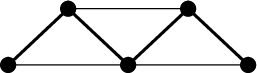 |
| graph | graph |
Suppose that the convex function is expressed as
| (6) |
where is a one-dimensional function. The potential of the form (6) is called additive. Then, the associated score is -local. Indeed, the score obtained from (6) is
| (7) |
which depends on through .
The Bregman divergence for associated with the -local potential (4) defined from the collection of local potentials is expressed as
| (8) |
The derivation is shown in the Appendix A. In the derivation of the above equality, we use the formula
for any .
The undirected graph determining the neighborhood system and the collection of local potentials lead to the Bregman divergence as the sum of localized Bregman divergences . Here, let us define the composite local Bregman divergence.
Definition 3 (Composite local Bregman divergence).
Let be a subset of and be an undirected graph that determines the neighborhood . Each point has a local potential . For a collection of local potentials , the composite local Bregman divergence is defined as
| (9) |
In the above definition, the subset rather than the whole sample space is introduced as the general expression.
The 1-homogeneous potential of is given by
The gradient of the above potential leads to the proper homogeneous score,
| (10) |
for . The derivation of (10) is shown in the Appendix B. Conversely, any proper homogeneous score is expressed by using the (sub)gradient of a -local potential with some graph . A trivial expression is given by using a singleton and the complete graph .
In the sequel sections, we investigate the condition of the graph and the collection of local potentials such that the proper homogeneous score becomes to be strictly proper.
4 Coincidence Axiom and Neighborhood Systems
In order to use the score to statistical inference, strictly proper scores are favorable rather than just proper ones. The Bregman divergence associated with the strictly proper score satisfies the coincidence axiom on , i.e.,
Firstly, we consider a sufficient condition of the coincidence axiom when the function set
includes only strictly convex functions. Secondly, we consider the case that ’s are convex but not strictly convex. In particular, we consider the case that is the potential defined as the localized variant of the pseudo-spherical divergence in Example 4.
4.1 Strictly Convex Local Potentials
Suppose that all local potentials in are strictly convex. We assume that the composite local Bregman divergence (9) vanishes, i.e., for . Then, due to the positivity of for all , each term should be zero. The strict convexity of the potential leads to for all . Hence, we have
for all and all . If there exists a point for some , we have . This implies that all ’s are the same for if for .
On the basis of the above result, we give a sufficient condition that the composite local Bregman divergence satisfies the coincidence axiom on .
Theorem 3.
Suppose that the neighborhood system of the sample space is determined by the undirected graph . For a subset of , we assume
Let us define the graph as
We assume that the graph is connected and all functions in are strictly convex. Then, the composite local Bregman divergence satisfies the coincidence axiom on .
Proof.
Assume that for . The assumption of the theorem guarantees that for any , there exist satisfying and . Thus, we have and as shown above. Since is connected, there is a path in such that . The argument just before Theorem 3 guarantees the equations,
This implies the probabilities and are linearly dependent. Hence, they should be the same. ∎
The similar argument of the above proof was presented in [19] to prove that the ratio matching score is strictly proper. Note that for leads to the linear dependency of and . Even if strict convexity is locally assumed, the coincidence axiom on is not guaranteed in general.
The following theorem shows that the connectedness of is closely related to that of .
Theorem 4.
If is connected, is connected. If holds, the connectedness of is equivalent with that of .
Proof.
Let us assume that is connected. Then, for any , there exists a sequence of points such that holds for all . Hence, for the point , we have . Since the sequence of the points connects and , we find that is connected.
Let us prove the later part of the theorem. Suppose that is connected. Then, for any , there exist a sequence of points such that holds for all . Hence, we have for , meaning that is connected. ∎
4.2 Local Pseudo-spherical Potential
Here, let us consider the case that the convex function is not strictly convex. In particular, we assume that all ’s are the localized version of the pseudo-spherical potential shown in Example 4. More precisely, the local pseudo-spherical potential is defined as the norm on , i.e.,
for a positive constant . Since holds for , is not strictly convex. Let on be the Bregman divergence defined from . Suppose that holds for . Then, and are linearly dependent as shown in Example 4.
Let be the composite local Bregman divergence defined from the local pseudo-spherical potentials.
Lemma 1.
Suppse that holds for . If for some , all ’s are the same for .
In this case, is not guaranteed.
Proof.
When holds for , the positivity of leads to for all . Thus, and are linearly dependent, meaning that there exists such that for all (not ) and all . For , we have . This implies that all ’s are the same for if for some . ∎
On the basis of the above Lemma, we give a sufficient condition that leads to on .
Theorem 5.
Suppose that the neighborhood system of the sample space is determined by the undirected graph . For a subset of , we assume
Let us define the graph as
We assume that the graph is connected and all functions in are pseudo-spherical potentials. Then, the composite local Bregman divergence satisfies the coincidence axiom on .
Proof.
Assume that for . For any , there exist satisfying and . Since is connected, there is a path in such that . Choose a vertex for each . Lemma 1 guarantees
This implies the and are linearly dependent. For probability vectors, they should be the same. ∎
Let us show a simple example that illustrates how the sufficient condition affects the strict convexity of the composite local Bregman divergence. The sample space is given as the binary variables , and the Hamming distance on is defined as the number of components at which the corresponding symbols are different, i.e.,
for and . Let us define the neighborhood system as
For , the pseudo-spherical penitential with this neighborhood system does not produce the strictly proper score. For , the probabilities
satisfy and . Thus, we have though . If the neighborhood system of is replaced with
the corresponding local homogeneous score is strictly proper. Indeed, when holds for two dimensional binary variables in , the edge connecting and leads to the additional constraint , etc. As a result, we obtain .
5 Examples
We show pseudo-likelihood [5], composite likelihood [23], ratio matching [19], local density-power score and local pseudo-spherical score as examples of proper local homogeneous scores. Usually, the pseudo-likelihood, composite likelihood and ratio matching are defined for the probability over the multidimensional binary vector space. In our formation, they can be defined on any discrete sample space endowed with the graph-based neighborhood system.
In the following examples, we assume .
5.1 Pseudo-likelihood
The pseudo-likelihood is a common estimation method that does not require the computation of normalization constant [5]. Usually, the pseudo-likelihood is used for multidimensional discrete samples such as . For the sample , we define as the dimensional vector . For the random variable taking a value in , the sub-vector is defined in the same way. The pseudo-likelihood for the sample is defined as
where denotes the conditional probability of given .
When the statistical model (3) on is used, the normalization constant is not needed to compute the pseudo-likelihood. The set of edges of the graph is given as
where is the Hamming distance on . Then, the adjacents of is
The event, , is the same as . The statistical model is defined by
where is the parameter to specify the probability. The logarithm of the pseudo-likelihood is expressed as
Hence, the score of the pseudo likelihood is given as
| (11) |
The corresponding local potential is
which is -local, additive and strictly convex on . One can confirm that the equality (7) holds. The composite local Bregman divergence is
Theorem 3 guarantees that the above composite local Bregman divergence satisfies the coincidence axiom on . The set can be replaced with , while keeping the score (11) to be strictly proper.
Even for the general discrete sample space , the pseudo-likelihood defined by the score (11) is strictly proper when the neighborhood system is properly defined.
5.2 Composite Likelihood and its Extension
Composite likelihood (CL) was proposed as an extension of the pseudo-likelihood in order to improve the efficiency [23]. Let the sample space be and the sample is denoted as . For a collection of subsets , we define as the sub-vector of . The CL for the sample is defined as
| (12) |
where is the complement of the set . The standard pseudo-likelihood is obtained by setting for . The condition can be expressed as the neighborhood system on . Let us define the graph as
Then, we have the following theorem.
Theorem 6.
Suppose . Then, the undirected graph determined from is connected if and only if
| (13) |
holds.
Proof.
Theorem 4 guarantees that the connectedness of is equivalent with that of when holds. Firstly, we assume (13). Let and be arbitrary points in , and suppose . There exists an index set that includes , meaning that the point is an adjacents of . By repeating this process, we can confirm that there exists a path connecting and in the graph .
Conversely, let us assume that . Then, we have . This means that the two points, and , can be adjacents to each other only when . If , a path connecting and does not exist. ∎
We define the subset by
Then, we have . The score of the CL is expressed as
The potential is obtained by on . The set of local potentials, , is given as
| (14) |
The above may not be strictly convex. We show a sufficient condition such that is strictly convex on . For the subset , let us define the vector as for and for .
Theorem 7.
The local potential (14) is strictly convex on if the rank of the by matrix is .
Proof.
A simple calculation yields that the Hessian matrix of is given as the by matrix
For a column vector , we suppose that . Then,we have
If the condition of the theorem holds, we have . Hence, the Hessian matrix of is positive definite and the function is strictly convex. ∎
The rank condition in Theorem 7 and (13) is not directly related to each other as shown in the following example.
Example 5 (Rank condition).
The homogeneous score given by the gradient of the potential is expressed as
| (15) |
at , where and for denotes the conditional probability of the probability . For the multidimensional binary space with the above neighborhood system, we have
Thus, we obtain
Therefore, the second and third terms in (15) cancel out, and the standard CL is obtained. Though the local potentials are not additive, the score becomes -local.
Let us define an extension of the CL on the general sample space that is not necessarily the multidimensional binary space. Suppose that the neighborhood system is determined from an undirected graph , and be subsets of such that holds. Then, (15) is a -local homogeneous proper score on the general sample space . Note that the second and third terms in (15) will not cancel out. Thus, we need to use the proper -local score (15) instead of the standard -local CL.
Let us summarize the theoretical properties of the extended CL. Suppose that the rank condition in Theorem 7 is satisfied and that the undirected graph is connected. Then, Theorems 3, 4, and 7 guarantees that the score (15) is strictly proper, -local, and homogeneous. Note that Theorem 7 works for any discrete sample space .
Example 6.
Suppose . For the pseudo-likelihood, the sets in (12) is given by and the rank condition in Theorem 7 is satisfied. As the another example, let us define the sets as and with if is even. Then, the rank condition in Theorem 7 holds. Similar result holds for the odd . As shown in Proposition 7.1 of [7], the standard CL (12) is strictly proper if
| (16) |
holds. The rank condition in Theorem 7 is more strict than (16). Under the condition (16), the convexity of local potentials is not guaranteed, but the score becomes strictly proper. On the other hand, the rank condition is a sufficient condition for the local potential to be strictly convex. An advantage of the rank condition is that it is available for any discrete sample space.
We consider the sufficient condition under which (15) on the general sample space is reduced to the form of the standard CL. When holds for any , the neighborhood system determined from is called the equivalence function [21]. Suppose that is the equivalence function for all . In the same way as the case of , one can prove that (15) is reduced to the -local CL
on the general sample space . In [21], the equivalence function is used without referring to the relation between -local and -local scores.
5.3 Ratio Matching
Suppose that the sample space is defined as and that two points in are adjacents to each other if the Hamming distance between them is equal to one. The neighborhood system is determined by such . The score of the ratio matching is defined as
| (17) |
which is -local. The normalization constant of the probability is not needed to compute due to the ratio . The corresponding local potential is
which is -local, additive and strictly convex on . One can confirm that the equality (7) holds. The composite local Bregman divergence is
The strict convexity of and ensure that the assumptions of Theorem 3 hold. Hence, the above composite local Bregman divergence satisfies the coincidence axiom on . Even for the general discrete sample space , the ratio matching using (17) is strictly proper whenever the graph is connected.
5.4 Local Density-Power Score
Below we present the strictly proper local homogeneous score defined from the density-power potentials in Example 3. For the graph that determines the neighborhood system of the discrete sample space , let us define the -local additive potential as
for a fixed positive constant . The potential is strictly convex. The local homogeneous score defined from with is
which is -local. The composite local Bregman divergence is given as
Theorem 3 guarantees that the coincidence axiom on holds if is connected. Accordingly, the above homogeneous score is strictly proper.
5.5 Local Pseudo-spherical Score
We show the explicit expression of the local pseudo-spherical score. For the graph that determines the neighborhood system of a discrete sample space , let us define the -local potential as
This potential is convex but not strictly convex on . Moreover, is not additive. Hence, the corresponding score is not -local but -local in general. The score derived from the above potential is given as
and the composite local Bregman divergence is
Whenever the neighborhood system is properly defined, satisfies the coincidence axiom on and the corresponding local homogeneous score is strictly proper.
Let us consider the local pseudo-spherical score on . The undirected graph is defined such that if and only if , meaning that the neighborhood system of is expressed as the -dimensional hyper-cube. Suppose . Then, it is clear that the assumptions on the graph in Theorem 3 are satisfied. The first assumption in Theorem 5, , also holds. Let us consider the second condition of Theorem 5, i.e., the connectedness of . We see that if and only if is equal to . Suppose that are connected by a path in . Then, we have . If is odd, there does not exist a path connecting and in . As a result, is not connected. Indeed, has two disjoint components. The two components are expressed by
where is a fixed point. By adding an edge in between and , we obtain a connected graph. In order to obtain strictly proper local homogeneous scores from local pseudo-spherical potentials, we need to define the neighborhood system carefully.
6 Classification
Let us consider classification problems. Suppose that i.i.d. samples are observed from the probability distribution , where is a domain of feature and is a finite label set. Our goal is to estimate the conditional probability or to predict the label of a newly observed . We assume the statistical model of the conditional probability
where and is the parameter of the model. When the size of the label set is large, the computation of is intractable. The proper local homogeneous score is used in order to avoid the computation of the normalization constant.
The score is applicable for the estimation of the conditional probability. Let be the expectation with respect to the distribution of the feature . When is used to fit the data, the empirical mean of the proper homogeneous score satisfies
The minimization of the empirical score with respect to the unnormalized model is expected to provide a good estimator of up to a constant factor.
7 Simulations
We performed numerical experiments to investigate how scores and neighborhood systems affect estimation accuracy. In the first experiment, We used the fully-visible Boltzmann machine as the statistical model to estimate probability functions. Next, we consider the classification problems with a small label set to study the relation between neighborhood system and prediction accuracy.
7.1 Boltzmann Machines
In the experiments, the sample space was the multidimensional binary variables . The fully-visible and fully connected Boltzmann Machine (BM) on is the statistical model defined as
where is the -dimensional column vector. The model parameter is the by symmetric matrix. For large , the computation of is intractable. When -dimensional i.i.d. samples are observed, our task is to estimate the parameter such that approximates the probability distribution of the samples.
To estimate the parameter , the unnormalized model
is used with proper local homogeneous scores in order to circumvent the computation of the normalization constant. The estimator of is obtained as the minimum solution of empirical score,
In the experiment, we used the pseudo-likelihood (PL), ratio matching (RM), local pseudo-spherical (PS) score as proper local homogeneous scores. The parameter in the pseudo-spherical score was set to and . We examined two neighborhood systems determined by the Hamming distance , one is and the other is .
We estimated the parameter for and . The sample size was set to and . When , the maximum likelihood estimator was also computed. In order to evaluate the accuracy of the estimator , the negative log-loss, , was computed on the test samples . Here, the logarithm of the normalization constant was approximated by using the annealed importance sampling(AIS) [30]. Though the AIS is available to obtain an approximation of of a single parameter , using the AIS in the optimization process is computationally impractical.
In the first setup, the training and test samples were generated from the probability distribution defined by the Boltzmann machine, meaning that the statistical model was correct. We generated the random matrix , where each element of was independently distributed from the standard normal distribution. Then, the training and test samples were sampled from the probability by using the Markov chain Monte Carlo (MCMC) method [1] with the transition probability for . The burn-in period was set to . The size of the test samples was fixed to . The experiments were repeated 20 times. In each repetition, the different matrix was used. The averaged negative log-loss was calculated to evaluate the accuracy of the estimator for each estimation method.
The mean and standard deviation (sd) (resp. median and median absolute deviation (mad)) of the averaged negative log-loss was shown in the top (resp. bottom) panel of Table 1. The negative log-loss for the uniform distribution, i.e., , was also presented in the bottom line. When and , the mean value of the averaged loss was extremely large and the median stays small. It means that the averaged loss can become extremely large for a certain matrix . The estimator using samples took into account the wider range of the sample space than the estimator using samples. As a result, the accuracy was much improved. About the neighborhood system, the estimator using the neighborhood was superior to that using the neighborhood . For the pseudo-likelihood, Liang and Jordan proved that the wider neighborhood leads to more accurate estimator under some conditions [21]. We numerically verified that not only the pseudo-likelihood but also the ratio matching score has the same tendency.
The estimation accuracy of the local PS score was comparable to the other methods with . Though the local PS-score with the neighborhood system is not strictly proper on the set of all probabilities over , it might be strictly proper on smaller models such as Boltzmann machines. In addition, the estimation accuracy of the local PS score was not significantly affected by the choice of . This will be because the statistical model was well-specified, and the local PS score with any provides a consistent estimator for Boltzmann machines.
In the second setup, the handwritten data called “Optical Recognition of Handwritten Digits Data Set” in UCI repository [22] was used as training and test datasets. The handwritten data has 5620 samples, 64 features, and each sample has one label in . Each feature takes an integer ranging from to . In the experiment, the feature vector in was converted into the binary sample in by changing to and to , and the Boltzmann machine was used as the statistical model. Here, the class label was ignored and the probability distribution of the converted features was estimated. The training sample size was set to and , and the rest were used as test samples. We chose features out of 64 features. In the same way as the first setup, we examined the PS, RM, and local PS score to estimate the parameters, and the estimation accuracy was evaluated by the negative log-loss on the test samples. The AIS was used for the computation of the test loss.
Table 2 shows the mean value of the averaged negative log-loss for each estimator with the standard deviation. In this case, the median was almost the same as the mean. By comparing the result for and , we find that the estimator using the wider neighborhood achieved a higher accuracy particularly in the case of . In the local PS score, the choice of significantly affected the estimation accuracy. In the second setup, the statistical model will not be well specified. Thus, the estimation bias depended on the parameter . In practical data analysis, one needs to choose the parameter carefully.
| mean (sd) | ||||||||
|---|---|---|---|---|---|---|---|---|
| MLE | 1.491 (0.642) | 1.624 (0.667) | – | – | – | – | ||
| PL: | 4.273 (5.713) | 1.752 (0.779) | 40.577 (86.027) | 4.480 (5.226) | 41.839 (93.027) | 6.393 (3.897) | ||
| PL: | 1.700 (0.888) | 1.646 (0.664) | 26.409 (66.334) | 2.682 (2.639) | 36.205 (89.569) | 4.295 (2.773) | ||
| RM: | 4.277 (5.715) | 1.755 (0.787) | 39.707 (84.838) | 4.528 (5.740) | 40.917 (89.778) | 6.365 (4.144) | ||
| RM: | 3.481 (5.275) | 1.652 (0.660) | 38.264 (85.522) | 3.940 (4.964) | 40.464 (93.362) | 5.521 (3.620) | ||
| PS(): | 3.744 (5.482) | 1.675 (0.687) | 38.993 (83.623) | 4.471 (5.849) | 38.478 (87.264) | 5.497 (3.159) | ||
| PS(): | 4.014 (5.698) | 1.756 (0.754) | 39.670 (84.260) | 4.384 (5.409) | 40.370 (95.292) | 6.243 (3.835) | ||
| median (mad) | ||||||||
| MLE | 1.413 (0.720) | 1.604 (0.890) | – | – | – | – | ||
| PL: | 1.669 (1.154) | 1.667 (0.958) | 5.614 (5.451) | 2.435 (1.050) | 11.578 (9.743) | 4.934 (1.799) | ||
| PL: | 1.445 (0.901) | 1.628 (0.874) | 3.083 (1.566) | 2.056 (0.679) | 6.108 (2.719) | 3.735 (1.626) | ||
| RM: | 1.657 (1.179) | 1.683 (0.921) | 4.390 (3.787) | 2.502 (0.805) | 10.544 (8.494) | 5.606 (2.109) | ||
| RM: | 1.459 (0.907) | 1.623 (0.877) | 4.361 (3.776) | 2.251 (0.547) | 8.364 (5.477) | 4.721 (3.263) | ||
| PS(): | 1.452 (0.937) | 1.666 (0.898) | 3.903 (3.091) | 2.360 (1.117) | 9.438 (7.153) | 4.752 (2.900) | ||
| PS(): | 1.453 (1.026) | 1.663 (0.948) | 4.761 (4.173) | 2.430 (1.451) | 7.452 (5.648) | 4.795 (2.326) | ||
| uniform dist. | ||||||||
| MLE | 2.986 (0.029) | 2.954 (0.021) | – | – | – | – | ||
|---|---|---|---|---|---|---|---|---|
| PL: | 3.009 (0.175) | 2.959 (0.024) | 4.703 (0.568) | 4.467 (0.057) | 25.938 (13.716) | 21.163 (7.706) | ||
| PL: | 2.997 (0.035) | 2.963 (0.027) | 4.620 (0.110) | 4.473 (0.062) | 19.937 (11.421) | 13.104 (6.164) | ||
| RM: | 3.018 (0.191) | 2.969 (0.025) | 4.969 (1.012) | 4.505 (0.067) | 23.640 (13.171) | 18.503 (7.623) | ||
| RM: | 2.999 (0.038) | 2.963 (0.026) | 4.625 (0.123) | 4.475 (0.057) | 21.051 (11.180) | 14.188 (6.026) | ||
| PS(): | 3.062 (0.127) | 2.998 (0.069) | 4.665 (0.116) | 4.488 (0.061) | 19.091 (9.907) | 13.296 (5.443) | ||
| PS(): | 3.046 (0.198) | 3.013 (0.067) | 6.345 (1.070) | 5.487 (0.929) | 84.557 (23.407) | 63.777 (21.563) | ||
7.2 Classification
In this section, we used the scores to classification problems. The handwritten data in the previous section was again used. The data had 5620 samples, 64 features, and 10 labels. This time, the features were not reduced to the binary, i.e., the original features were used. Since the data has only 10 labels, the local homogeneous score is not needed to reduce the computational cost. Here, we investigate the influence of the neighborhood system to the prediction accuracy in classification problems. Using the training data , the conditional probability of the label given the input vector was estimated. The statistical model for the conditional probability was defined as
where
The dimension of the model parameter is 640. The model is overparametrized, i.e., the different parameter can specify the same conditional probability. The estimator was evaluated by the prediction error rate and negative log-loss on the test samples.
The neighborhood system introduced on is defined as
where for labels is computed as the difference of integers. We used the neighborhood system with and . We examined the MLE, PL, RM, local PS score, composite likelihood (CL) and modified composite likelihood (mCL) in (15). The CL with the above neighborhood system does not leads to proper score on . In order to guarantee the consistency of the estimator, we need to use the mCL instead of the CL.
The signal to noise ratio of the original data is very low and the estimator of the conditional probability tends to overfit to training data. In this experiment, we added artificial noise to the data. Concretely, 10 or 20 samples were picked up, and their labels were replaced according to the uniform distribution on . The training sample size was set to and , and the rest were used as test samples. We randomly split the dataset into training and test sets, and repeated the experiments 100 times.
The results are presented in Figures 2 and 3. Overall, the MLE achieved the highest accuracy. The estimators with the wider neighborhood were superior to those with . Under the test error of the label, the local PS score with (PS:2) provided the better classifier than the other local scores. The negative log-loss of the PL, CL and mCL with (PL:2, CL:2, and mCL:2) was smaller than the other local homogeneous scores. This is because, the empirical loss to be minimized in the learning is close to the negative log-loss for the evaluation. In this experiment, the CL and mCL showed almost the same accuracy. The efficiency of the local PS score was less than that of the PL, CL and mCL.
 |
 |
 |
 |
 |
 |
 |
 |
8 Conclusion
In this paper, we study strict properness of local homogeneous scores through the coincidence axiom for composite local Bregman divergences on discrete sample space. The connectedness of the neighborhood graph is important to derive strictly proper local homogeneous scores. The consistency of some existing scores and newly proposed ones is investigated. Some numerical experiments are conducted to investigate how neighborhood systems affect the estimation accuracy.
There are several directions to be further explored in the future. It is of great interest to study the efficiency and robustness of local scores. More precisely, how the estimation accuracy and robustness of the estimator relates to the neighborhood system, local potential and statistical models. In the numerical experiments in Section 7.2, the efficiency of the local PS score was inferior to that of the pseudo-likelihood and composite likelihood. However, the local PS score may provide a robust estimator as well as the standard PS score used in robust statistics [12] instead of providing an efficient estimator. Another important research direction is to improve the computational efficiency. Though the computation cost of local scores are much smaller than the MLE, the standard optimization solver is still insufficient for the statistical analysis of extremely massive data using huge models. Developing efficient optimization algorithms is needed in the big-data era.
Appendix A Derivation of (8)
Lemma 2.
The equality
holds for any .
Proof.
Since is equivalent with , we have
∎
Appendix B Score of Composite Local Bregman Divergence
Let be a set of local potentials. The associated composite local Bregman divergence is given as follows.
Therefore, the expected score is given by
Then, we obtain
Therefore, we have
When the local potential is expressed as the additive form , we have
For , we have
where .
References
- [1] C. Andrieu, N. de Freitas, A. Doucet, and M. I. Jordan. An introduction to MCMC for machine learning. Machine Learning, 50(1-2):5–43, 2003.
- [2] A. U. Asuncion, Q. Liu, A. T. Ihler, and P. Smyth. Learning with blocks: Composite likelihood and contrastive divergence. In Yee W. Teh and D. M. Titterington, editors, Proceedings of the Thirteenth International Conference on Artificial Intelligence and Statistics (AISTATS-10), volume 9, pages 33–40, 2010.
- [3] A. Banerjee, S. Merugu, and J. Ghosh I. S. Dhillon. Clustering with bregman divergences. Journal of Machine Learning Research, 6:1705–1749, 2005.
- [4] A. Basu, I. R. Harris, N. L. Hjort, and M. C. Jones. Robust and efficient estimation by minimising a density power divergence. Biometrika, 85(3):549–559, 1998.
- [5] J. Besag. Spatial interaction and the statistical analysis of lattice systems. Journal of the Royal Statistical Society. Series B (Methodological), 36(2):192–236, 1974.
- [6] S. Boyd and L. Vandenberghe. Convex Optimization. Cambridge University Press, Cambridge, 2004.
- [7] J. K. Bradley and C. Guestrin. Sample complexity of composite likelihood. In In Artificial Intelligence and Statistics (AISTATS), La Palma, Canary Islands, April 2012.
- [8] L. M. Bregman. The relaxation method of finding the common point of convex sets and its application to the solution of problems in convex prog ramming. USSR Computational Mathematics and Mathematical Physics, 7:200–217, 1967.
- [9] M. Collins, R. E. Schapire, and Y. Singer. Logistic regression, adaboost and Bregman distances. In Proceedings of the Thirteenth Annual Conference on Computational Learning Theory, pages 158–169, 2000.
- [10] T. M. Cover and J. A. Thomas. Elements of Information Theory (Wiley Series in Telecommunications and Signal Processing). Wiley-Interscience, 2006.
- [11] A. P. Dawid, S. Lauritzen, and M. Parry. Proper local scoring rules on discrete sample spaces. Annals of Statistics, 40:593–608, 2012.
- [12] H. Fujisawa and S. Eguchi. Robust parameter estimation with a small bias against heavy contamination. J. Multivar. Anal., 99(9):2053–2081, 2008.
- [13] C. J. Geyer. Markov chain monte carlo maximum likelihood. Computing Science and Statistics: Proceedings of the 23rd Symposium on the Interface, pages 156–163, 1991.
- [14] T. Gneiting and A. E. Raftery. Strictly proper scoring rules, prediction, and estimation. Journal of the American Statistical Association, 102:359–378, 2007.
- [15] M. Gutmann and J. Hirayama. Bregman divergence as general framework to estimate unnormalized statistical models. In Proc. Conf. on Uncertainty in Artificial Intelligence (UAI2011), pages 283–290, 2011.
- [16] A. D. Hendrickson and R. J. Buehler. Proper scores for probability forecasters. The Annals of Mathematical Statistics, 42:1916â1921, 1971.
- [17] G. E. Hinton. Training products of experts by minimizing contrastive divergence. Neural Compututation, 14(8):1771–1800, 2002.
- [18] A. HyväÌrinen. Connections between score matching, contrastive divergence, and pseudolikelihood for continuous-valued variables. IEEE Transactions on Neural Networks, 18(5):1529–1531, 2007.
- [19] A. Hyvärinen. Some extensions of score matching. Computational Statistics & Data Analysis, 51:2499–2512, 2007.
- [20] T. Kanamori and H. Fujisawa. Affine invariant divergences associated with composite scores and its applications. Bernoulli, 20(4):2278–2304, 2014.
- [21] P. Liang and M. I. Jordan . An asymptotic analysis of generative, discriminative, and pseudolikelihood estimators. In Proceedings of the 25th International Conference on Machine Learning, ICML ’08, pages 584–591, New York, NY, USA, 2008. ACM.
- [22] M. Lichman. UCI machine learning repository, 2013.
- [23] B. G. Lindsay. Composite likelihood methods. Contemporary Mathematics, 80(1), 1988.
- [24] S. Lyu. Interpretation and generalization of score matching. In Proceedings of the Twenty-Fifth Conference on Uncertainty in Artificial Intelligence, UAI ’09, pages 359–366, Arlington, Virginia, United States, 2009. AUAI Press.
- [25] B. Marlin and N. de Freitas. Asymptotic efficiency of deterministic estimators for discrete energy-based models: Ratio matching and pseudolikelihood. In Uncertainty in Artificial Intelligence (UAI), Corvallis, Oregon, 2011. AUAI Press.
- [26] J. McCarthy. Measures of the value of information. Proc Natl Acad Sci U S A., 42(9):654–655, 1956.
- [27] N. Murata, T. Takenouchi, T. Kanamori, and S. Eguchi. Information geometry of -Boost and Bregman divergence. Neural Computation, 16(7):1437–1481, 2004.
- [28] M. Parry, A. P. Dawid, and S. Lauritzen. Proper local scoring rules. Annals of Statistics, 40:561–592, 2012.
- [29] M. Pihlaja, M. Gutmann, and A. Hyvärinen. A Family of Computationally Efficient and Simple Estimators for Unnormalized Statistical Models. In Proc. Conf. on Uncertainty in Artificial Intelligence (UAI), pages 442–449, Corvallis, Oregon, 2010. AUAI Press.
- [30] R. Salakhutdinov. Learning and evaluating boltzmann machines. Technical report, UTML TR 2008-002, Dept. of Computer Science, University of Toronto, 2008.