Galactic Gamma Ray Excess and Dark Matter Phenomenology in a Model
Abstract
In this work, we have considered a gauged extension of the Standard Model (SM) with three right handed neutrinos for anomaly cancellation and two additional SM singlet complex scalars with nontrivial B-L charges. One of these is used to spontaneously break the gauge symmetry, leading to Majorana masses for the neutrinos through the standard Type I seesaw mechanism, while the other becomes the dark matter (DM) candidate in the model. We test the viability of the model to simultaneously explain the DM relic density observed in the CMB data as well as the Galactic Centre (GC) -ray excess seen by Fermi-LAT. We show that for DM masses in the range 40-55 GeV and for a wide range of gauge boson masses, one can satisfy both these constraints if the additional neutral Higgs scalar has a mass around the resonance region. In studying the dark matter phenomenology and GC excess, we have taken into account theoretical as well as experimental constraints coming from vacuum stability condition, Planck bound on DM relic density, LHC and LUX and present allowed areas in the model parameter space consistent with all relevant data, calculate the predicted gamma ray flux from the GC and discuss the related phenomenology.
I Introduction
The presence of dark matter in the Universe is now well established. Its presence has been probed by its gravitational interaction with the visible world such as the rotation curve of spiral galaxies [1], gravitational lensing [2], and the phenomena of the Bullet cluster [3]. Meanwhile, the amount of dark matter present in the Universe has already been measured with an unprecedented accuracy by various satellite borne experiments like WMAP [4] and Planck [5]. The results of these experiments reveal that our Universe has more than 80% of its matter content in the form of dark matter while the remaining part is composed of known baryonic matter. However, the possible nature of the constituents of dark matter and their interactions with the Standard Model (SM) particles as well as with themselves still remains an enigma. As the Standard Model of particle physics does not have any fundamental particle which can play the role of a dark matter candidate, there exist many extensions of SM which can accommodate a single [6, 7, 8, 9, 10, 11, 12, 13, 14, 15, 16] or multicomponent dark matter scenarios [17, 18, 19, 20, 21, 22]. Out of these different types of dark matter scenarios the most favourable one is the class of particles known as weakly interacting massive particle or WIMP [23, 24]. This class of dark matter particles were produced thermally at early stage of the Universe and maintained their thermal as well as chemical equilibrium through the interactions with other particles within the thermal plasma. As the Universe expanded and cooled down their rates began to decrease and eventually, when the annihilation rate of WIMP became less than the expansion rate of the Universe, WIMP decoupled from the thermal plasma and froze to a particular relic density.
Particle nature of WIMP can be explored mainly in two possible ways. First is the method of direct detection, where the information about WIMP mass and the nature of its interaction with SM particles can be obtained by measuring the recoil energy of the detector nuclei scattered by the WIMP. There are many ongoing dark matter direct detection experiments such as LUX [25, 26], XENON1T [27] and SuperCDMS [28]. However, none of them have observed yet any “real event” which is produced by the scattering of dark matter particles with the detector nuclei and have thus placed an upper bound on both the spin independent and spin dependent scattering cross sections of WIMP as a function of its mass. Another promising method is the indirect detection of dark matter, where the detection of annihilation products of gravitationally bound dark matter particles within the core of massive celestial objects like the Sun, galaxies, galaxy clusters and dwarf galaxies can provide viable information about the particle nature of dark matter. These annihilation products include high energy neutrinos, gamma-rays and charged cosmic rays (electrons, positrons, protons and antiprotons) [29]. Among these annihilation products gamma-rays and neutrinos play an important role as they propagate through these celestial objects unperturbed and thereby directly point towards their sources.
Recently, several groups have reported [30, 31, 32, 33, 34, 35, 36, 37, 38, 39, 40] an excess in gamma-ray flux in the energy range GeV by analysing the Fermi-LAT publicly available data [41]. These analyses reveal that the observed gamma-ray flux originates from the inner few degrees around the centre of our Milky Way galaxy and the nature of this excess gamma-ray spectrum is compatible with that produced by the annihilation of WIMP dark matter in the Galactic Centre (GC) region. Although, there are astrophysical explanations of this anomalous gamma-ray excess in terms of unresolved point sources (e.g. millisecond pulsars) around the GC [42, 43], in this work we consider a dark matter explanation of the GC gamma-ray excess. In Ref. [40], the authors have shown that this observed gamma-ray flux can be well explained by an annihilating self-conjugate dark matter of mass around GeV with an annihilation cross section cms for the annihilation channel. In this analysis they have used an NFW [44] dark matter halo profile with and local dark matter density GeVcm3. Moreover, the authors of Ref. [40] have considered a region where galactic longitude and latitude vary in the range and respectively as the region of interest (ROI) for their analysis. It is also mentioned in Ref. [40] that the uncertainties in the “astrophysical J factor”, due to our poor knowledge about DM halo profile parameters, can change the best fit DM annihilation cross section by a multiplicative factor which varies in the range [0.17,5.3]. Various particle dark matter models explaining the Galactic Centre gamma-ray excess are available in Refs. [45, 46, 47, 48, 49, 50, 51, 52, 53, 54, 55, 56, 57, 58, 59, 60, 61, 62, 63, 64, 65, 66, 67, 68, 69, 70, 71, 72, 73, 74].
In this work, we consider an extension of the SM where the gauge sector of SM is enhanced by a local gauge group where B and L represent the baryon and lepton numbers respectively. In this model we have an extra neutral gauge boson as the model Lagrangian possesses an additional local gauge invariance. In order to construct an anomaly free theory, the model needs three right handed neutrinos with charge equal to . Thus, extension of the SM is a well motivated beyond Standard Model (BSM) theory which can explain the origin of tiny neutrino masses through the type-I seesaw mechanism. Majorana mass terms of these three right handed neutrinos are generated in a gauge invariant way by introducing a SM gauge singlet scalar having charge . The gauge symmetry breaks spontaneously when the scalar field gets a vacuum expectation value , thereby generating mass of the gauge boson and the right handed neutrinos. The mixing between the neutral components of and the SM Higgs doublet produces two physical scalars namely and where is identified as the SM-like Higgs boson with mass around 125.5 GeV. The extension of SM [75, 76, 77, 78] has been explored before in the context of dark matter phenomenology [60, 79, 80, 81, 82, 83, 84, 85, 86] and baryogenesis in the early Universe in Refs. [87, 88, 89]. In the present work we have introduced a complex scalar field to the extension of SM. This complex scalar field is singlet under the SM gauge group while it transforms nontrivially under gauge group. By choosing proper charge, this scalar field can be made stable and hence it can play the role of a viable dark matter candidate. In this present work, we have considered the low mass region GeV to GeV of DM masses to explain the Fermi-LAT gamma-ray excess from the Galactic Centre, whereas the high mass region has been studied in Ref. [85]. We have calculated the relic density of by solving Boltzmann equation numerically. We have found that the gamma-ray flux produced from the annihilation of and can reproduce the gamma-ray excess as observed by Fermi-LAT from the direction of GC. Moreover, in this work, we have taken into account all the possible existing theoretical as well as experimental constraints obtained from experiments like LHC, LEP, LUX, Planck.
The paper is arranged in the following way. In Section II we describe the model in detail and discuss the constraints on it from different experiment. In Section III we calculate the relic density in this model. In Section IV we show the variation of the relic density with different model parameters. In Section V we explain the Fermi-LAT gamma-ray excess. Finally in Section VI we conclude.
II Model
In the present work, we have considered “pure” extension of the Standard Model (SM) of elementary particles where the SM gauge group is enhanced by an additional local gauge symmetry where B and L represent the baryon and lepton numbers, respectively. Therefore, all the SM (quarks and leptons) fields transform nontrivially under this gauge group. Besides the SM fields, we have to introduce three right handed neutrinos ( to 3) such that the present model becomes anomaly free. Further, in addition to the usual SM Higgs doublet , the scalar sector of the SM is also extended by adding two SM gauge singlet complex scalar fields, namely , both of which possess nonzero charge. gauge symmetry breaks spontaneously when the scalar field gets a nonzero vacuum expectation value (VEV) . Consequently, we have one extra neutral massive gauge field in the model. Moreover, after spontaneous breaking of symmetry, the Majorana mass terms for the three right handed neutrinos can be generated in a gauge invariant way by choosing a suitable charge of the scalar field . Also, if the value of the relevant model parameters are such that the VEV of is zero then the complex scalar field can be made stable by giving an appropriate to it. Under such circumstances can be a viable dark matter candidate. The charges as well as the SM gauge charges of all the fields present in the model are given in a tabular form (see Table 1).
|
|
|
| ||||||||||||||||||||||||||||||||||||||||||||||||||
The Lagrangian of the present model including the SM Lagrangian is as follows
| (1) | |||||
with , while represents the dark sector Lagrangian whose expression is given by
| (2) | |||||
and the self interactions of and its mutual interaction with the SM Higgs doublet are described by which can be written as
| (3) |
In Eq. (1), is the field strength tensor of the gauge field . Covariant derivative appearing in Eqs. (1, 2) is defined as
| (4) |
where , , and is the corresponding gauge charge which is given in Table 1. In general, the Majorana mass matrix for the three right handed neutrinos, obtained after spontaneous breaking of symmetry, will contain off diagonal terms. However these off diagonal terms can be easily removed by changing the basis and therefore, we have considered the diagonal Majorana mass matrix for the three right handed neutrinos (or the right handed neutrinos ’s are in mass basis).
After spontaneous breaking of symmetry the scalar fields and in unitary gauge take the following form
| (5) |
where is the VEV of , which breaks the electroweak symmetry to a symmetry (). On the other hand the VEV of , , is responsible for the breaking of gauge symmetry of the Lagrangian and thereby generates masses for the three right handed neutrinos as well as the gauge boson ,
| (6) |
In Eq. (5) and are two neutral scalar fields of and respectively. There is also mixing between and through the term (see Eq. (3)). As a result, the mass matrix of and contains off diagonal elements which are proportional to , and . Hence, and are not representing any physical field. The scalar mass matrix with respect to the basis is given by
In order to obtain the physical states we have to diagonalise the real 11 1 In present model we have taken all the coupling constants and VEVs as real. symmetric matrix (Eq. (II)) by an orthogonal matrix. The physical fields or the mass eigenstates which are linearly related to and , can be obtained through the following relations
| (11) |
where the scalar field is identified as the SM like Higgs boson and is the extra Higgs boson in the model, while is the mixing angle between and given as
| (12) |
We will see later that from LHC results, the allowed values of the mixing angle are extremely small. The expressions of masses of the three physical scalar fields , and are
| (13) |
Since is the SM like Higgs boson therefore we have taken GeV.
In this model, besides the SM parameters, we have twelve unknown independent parameters, namely the masses of , , , , gauge coupling , charge () of dark matter (), scalar mixing angle and three quartic couplings , , . In terms of these independent parameters, the couplings appearing in the Lagrangian (Eqs. (1-3)) can be expressed as
| (14) |
where and are the quadratic self coupling of the SM Higgs doublet and the extra Higgs singlet respectively. Moreover, the model parameters are subjected to satisfy certain conditions arising from theoretical constraints as well as relevant experimental results. These constraints are briefly discussed below.
- •
Vacuum Stability: In our model we choose the ground state (, , ) = (, , 0). This requires the following constrains on the quadratic self couplings of the scalar fields,
(15) Also in order to obtained a stable ground state (vacuum), the quartic couplings, appearing in the Lagrangian, need to satisfy the following conditions
(16) - •
Planck Limit: The relic density of the dark matter particle at the present epoch should lie within the range reported by the satellite borne experiment Planck [5], which is
(17) - •
Stability of dark matter: We give a charge to the dark matter candidate () in such a way so that all possible decay terms are forbidden by the invariance of gauge symmetry which therefore ensures the stability of . In general, the possible decay terms of are like (where and , are integer can vary from to ) and , where is and 22 2 Since is singlet under SM gauge group therefore a term like with being any Standard Model fermion is forbidden.. From Table 1 one can see that the charges of and are 0 and +2 respectively. Therefore if we take then we can not write the term , as it will violate the gauge symmetry. In addition, in our case, we have varied dark matter mass from GeV to GeV and 33 3 which is required to explain Fermi-LAT gamma excess [40], see section V for more detailed discussion. as a result any decay modes of to these scalar bosons are kinematically forbidden. Moreover, due to the presence of term, the dark matter candidate can also decay into two Majorana type right handed neutrinos in the final state, if the kinematical condition (, 1 to 3) is satisfied, which can also destroy its stability. To get rid of this decay term we can not choose as the combination has charge . Therefore, in order to avoid all the above mentioned decay terms (due to renormalizability of the Lagrangian we have considered operators only upto dimension 4) we need where is any integer between 0 and 3.
- •
LEP bound: Since the SM fermions are charged under the gauge group , therefore LHC should find some footprint of the gauge boson as it can directly interact with all the SM fermions. The nondetection of any signature of puts a severe constraint on its mass () and gauge coupling (). From LEP experiment the ratio is bounded from below by the following condition [90, 91] 44 4 Recent bounds on the mass and gauge coupling of from ATLAS collaboration are given in Ref. [92].
Figure 1: Feynmann diagrams for spin independent scattering cross section of dark matter particle/antiparticle with nucleon () through both Higgses () and gauge boson . - •
LUX limit: In this model, the complex scalar field is our dark matter candidate. Therefore, both and its antiparticle can elastically scatter off the detector nuclei through the exchange of neutral scalars , and gauge boson . Moreover, due to the presence of vector boson () mediator, the elastic scattering cross sections for the dark matter and its antiparticle are different. If we take the number densities of the dark matter and its antiparticle to be equal at the present epoch (which is true if the species has negligible chemical potential [23]), then we have to multiply the elastic scattering cross sections of dark matter and its antiparticle by a factor while comparing these scattering cross sections, obtained from the present model, with the experimental upper limits reported by the direct detection experiment LUX [25, 26]. The reason behind this is the exclusion regions in plane reported by different dark matter direct detection experiments are computed assuming the existence of only one type of dark matter particle (and also self-conjugate) in the Universe. Although our model too has only one kind of dark matter candidate, however, it has a different antiparticle and they do not possess equal interaction strengths with the detector nuclei. Feynman diagrams for the elastic scattering of both and with the nucleon () are shown in Fig. 1. These processes are mediated through the exchange of , and . The expressions of spin independent scattering cross sections off the nucleon () for both and are given by
(27) where is the vertex factor for a vertex involving fields (, 2) and its expression is given in Table 1. The reduced mass between nucleon (proton or neutron) and DM particle is denoted by . Moreover, the nuclear form factor for the scalar mediated processes is [93] while that for mediated diagram is 55 5 coupling [94] with is the coupling for the vertex containing fields (see Table 2). Now for proton (neutron ) () [94]. Therefore, for both the nucleon ( and ) the coupling with . Thus in this model form factors of proton and neutron are same for mediated diagram.. From the expression of spin independent scattering cross section it is seen that although, the elastic scattering cross sections of and with are identical when the scattering processes are mediated through the scalar bosons only, however, if we include the mediated diagram then the elastic scattering cross sections for both and become different from each other. It is due to the fact that the momentum dependent vertex factors for the vertices and 66 6 see the expression of in Table 2 are differ by a -ve sign (due to the change in sign of momentum while go from particle to anti particle scenario) from each other which results in a difference between and arising from the interaction terms between and scalar bosons mediated diagrams. If represents the upper limit of the spin independent scattering cross section reported by the LUX experiment for a particular dark matter mass then for a viable dark matter model both and must satisfy the following condition
(28) - •
LHC constraints:
- –
Signal Strength of SM-like Higgs: The signal strength of for a particular decay channel ( is any SM particle such as gauge boson, quark or lepton) is defined as
(29) where and are the production cross section of and its branching ratio for decay channel. In the denominator of the above equation represent the same quantities for the SM Higgs boson (). If the neutral boson is similar to the SM Higgs boson then according to LHC result the signal strength ratio should be 77 7 We have considered the central value of the combined signal strength of the SM Higgs boson reported by the CMS collaboration [95]. [95]. We will see later, in Fig. 3 (Section IV) that the above condition will impose severe constrain on the allowed values of scalar mixing angle .
- –
Invisible decay width of Higgs boson: In the present model, the SM like Higgs boson can decay into a pair of and if the kinematical condition is satisfied. Such decay channel is known as the invisible decay model of . The expression of partial decay width of into final state is
(30) where is the vertex factor for the vertex involving . Throughout this work we have considered the partial width of this invisible decay channel of to be less than 20% [96, 97] of its total decay width.
- –
- •
Fermi-LAT gamma excess from Galactic Centre: In order to explain the Fermi-LAT observed gamma-ray excess from the Galactic Centre using a self-conjugate annihilating dark matter, one needs a dark matter particle of mass GeV [40]. If we assume an NFW halo profile with , GeV/cm3, kpc and kpc then the annihilation cross section of dark matter particle for the annihilation channel should lie in the range cms [40]. However, if we take into account the uncertainties of DM halo profile parameters (mentioned above) then the quantity can vary in the range cm3/s with [40]. We will discuss about the Fermi-LAT gamma-ray excess elaborately in Section V where we will see that the required value of for a non-self-conjugate DM (which is true for the present model) is different from a dark matter candidate whose particles and antiparticles are same.
III Relic Density
The evolution of total number density () of both and is governed by the Boltzmann equation which is given by [23]
| (31) |
where is the Hubble parameter and is the equilibrium number density of both and . is the annihilation cross section for the channel , where is any SM fermion except top quark 88 8 In order to explain Fermi-LAT -ray excess we need in the range GeV [40] and thus other annihilation channels of (, , , , etc.) are not kinematically allowed.. Tree level Feynman diagrams for the process mediated through the exchange of , and are given in Fig. 2. The expression of is as follows,
| (32) | |||||
where is the total decay width of the particle (, , ), is the mass of the SM fermion and is centre of mass energy. is the vertex factor for the vertex involving the fields (, ) and its expression is given in Table 2. Moreover the quantity , with is the scalar mixing angle, is the coupling for the vertex (see Table 2). In Eq. (31), represents the thermal average of the product between annihilation cross section and the relative velocity of the annihilating particles. Extra factor appearing before is due to non-self-conjugate nature of [23]. Thermal averaged annihilation cross section can be defined in terms of annihilation cross section and modified Bessel functions () as [23]
| (33) |
where is the temperature of the Universe. Now, we define two dimensionless variables and as follows
with is the entropy density of the Universe while is called the total comoving number density of both and . In terms of these two variables the Boltzmann equation, given in Eq. (31), can be written as
| (34) |
where is the Newton’s gravitational constant and is a function of effective degrees of freedom related to both energy and entropy densities of the Universe [23]. Now, one can find the value of the total comoving number density () at the present temperature ( GeV) by solving the first order differential equation. The estimated value of is then used to compute the total relic abundance of both and at the present epoch through the following equation [98]
| (35) |
| Vertex | Vertex Factor |
|---|---|
IV Results
In this section we have shown how the relic density of DM varies with various model parameters namely , , , , , , , . In order to compute the DM relic density, we have solved the Boltzmann equation (Eq. (34)) numerically using the micrOMEGAs [99] package while the information of the present model is supplied to micrOMEGAs through the LanHEP [100] package. All the constraints on the model parameters, listed in Section II, are also taken into account in the numerical calculations.
In the left panel (right panel) of Fig. 3 we plot the variation of DM relic density with the scalar mixing angle for three different values of () (green dashed line), () (red solid line) and () (blue dashed-dotted line) while the values of other parameters are kept fixed at , GeV, GeV, GeV, () and . In this plot, magenta dotted line represents the central value of DM relic density as reported by the Planck collaboration (). From the Table 2 we see that the mediated diagram is independent of the mixing angle , so its contribution does not depend on . On the other hand the two Higgs scalars mediated diagrams are dependent on the mixing angle . It is seen from Fig. 3 that the dark matter relic density is practically independent of the mixing angle when becomes too small (). This can be explained as follows, in this region and the mediated diagram does not contribute since the vertex is suppressed and it is mostly the and mediated diagrams that contribute. For very small , even the mediated diagram is independent of since , making constant with . We also note from left (right) panel of Fig. 3 that in this region, has no dependence on (). This again can be explained using the fact that here only the mediated diagram (in addition to the mediated diagram which is anyway independent of , and ) contributes and Table 2 reveals that for small we have impact of only on .
On the other hand if we start increasing the mixing after the value (), the scalars and both start contributing along with gauge boson in the DM annihilation process, which enhances . Therefore the relic density which is approximately inverse of decreases with increase of mixing angle . Again we notice from Table 2 that the dependent term in the vertex and the dependent term in the vertex is proportional to . This makes the relic density decrease with increasing for larger values of , as is evident from the left panel of Fig. 3. Likewise the right panel shows the dependence of the relic density on which comes from the first term of the vertex. This explains the decrease of the relic density with . In this figure, we have also shown the excluded region for mixing angle from LUX and LHC experiment. The crossed region is excluded by both LUX and LHC experiment, whereas the forward lines is only excluded by LHC experiment.
Left panel of Fig. 4 represents the variation of with gauge coupling for three different chosen values of . Here green dashed-dotted line is for , red solid line is for whereas the plot for is shown by blue dashed line. Like the previous figures here also, the central value of Planck limit on DM relic density is indicated by magenta dotted line. It is seen from the left panel of Fig. 4 that initially the relic density increases with and attains a maximum value at , thereafter it starts decreasing with . The initial rise of , for low , is due to s channel process of , mediated by and . In this case, the relevant couplings (, 2) are inversely proportional to (see Table 2). However, as becomes large (), the other s channel process mediated by gauge boson starts dominating over the scalar exchange processes. From Table 2, one can easily see that the coupling is proportional to , which makes (via exchange) proportional to fourth power of 99 9 coupling is also proportional to .. The dominance of s channel exchange annihilation process over the scalar mediated ones is indicated by the fact that in this region (higher value of , ) (or ) does not depend on the coupling . We show by the hatched region the values of excluded by LEP.
In the right panel of Fig. 4 we show the variation of with the mass of the non-standard Higgs boson for three different values of its mixing angle with SM Higgs, namely , 0.05, 0.055. From this plot, it is seen that for all the chosen values of the relic density satisfies the Planck limit only near the resonance region when . The figure shows that in this region becomes practically independent of . We see that there are two sets of values of for which the model can predict the correct dark matter relic density. Of these two regions which are marked in the figure, one of them with GeV produces in the right ballpark value of , thus can explain the Fermi-LAT gamma-ray excess [40]. Whereas the other region labelled as “Region can’t explain Fermi-LAT excess” () produces (see Fig. 9 also).

Variation of with the mass of gauge boson is shown in left panel of Fig. 5. In this figure three different plots are computed for three different values of gauge coupling (). Here, red solid line is for while and are represented by green dashed line and blue dashed-dotted line, respectively. This figure is drawn for fixed values of other parameters, namely, , GeV, GeV, , , . From this plot it is seen that for a fixed value of , DM relic density increases with , which is consistent with the plot in left panel of Fig. 4 (cf. red line in the left panel of Fig. 4 where the maxima of occurs for ). The presence of resonance due to (when ) is also seen from this figure and like the previous case for here also the Planck limit is satisfied only near the resonance. However, the resonance due to is not as sharp as it is due to because in this region of parameter space the decay width of is nearly two orders of magnitude larger than that of . Here in the left panel the shaded region is not allowed by the LEP bound on . Right panel of Fig. 5 describes the variation of with the gauge charge () for three different values of neutral scalar mixing angle namely (blue dashed-dotted line), (red solid line) and (green dashed line), respectively. From this figure it is seen that as the charge of the DM candidate decreases, its relic density increases sharply and eventually the DM relic density saturates after a certain value of . A possible explanation of this nature of could be as follows. For large value of () the maximum contribution to DM annihilation cross section comes from gauge boson mediated channel as the cross section for this channel is directly proportional to . Hence becomes practically independent of the mixing angle . However as decreases from unity the scalar mediated s channel processes become significant and consequently after a certain value of () the annihilation cross section becomes nearly insensitive to and depends strongly on the mixing angle . In the right panel, we have given upper bound on the DM charge , which we get from LUX limit on spin independent direct detection cross section.
Variation of with dark matter mass for two different values of are shown in Fig. 6. In this figure, the left panel is for while the right panel is for . In each panel the three different lines represent the variation of with for three chosen values of , and respectively. From both panels of Fig. 6 it is seen that there are two resonance regions where the first one is for the non-standard Higgs boson ( GeV) while the second one corresponds to the SM Higgs boson of mass 125.5 GeV. In both panels the DM relic density satisfies the Planck limit (indicated by the magenta dotted line) only near the resonance regions. In both the panel of Fig. 6, we have shown allowed region of DM mass for explaining Fermi-LAT gamma-ray excess from GC.
We finally show the variation of with two remaining model parameters and in left and right panel of Fig. 7, respectively. In each panel we have shown the variation of for three different values of mixing angle namely , and . From the left panel of Fig. 7 it is seen that for small value of the parameter () relic density remains unaffected with respect to the change in value of as in this region DM annihilation cross section is controlled by the coupling which is considered to be . Also from Table 2 we see that when , the couplings and . However, the term within the modulus in Eq. (32) is proportional to . Therefore, inspite of being small in value, the variation of produces a significant change in and hence in relic density. Similarly, using Eq. (32) and Table 2 one can easily see that for higher value of (when ), the scalar mediated term in (term within modulus in Eq. (32)) mainly depends on and . Consequently, for the higher value of , there is no observable change in relic density with respect to and it decreases with the increase of . In right panel of Fig. 7 we have shown the variation of with . It is seen from this figure that, the behaviour of DM relic density with respect to the coupling is same as it is with i.e. initially for small value of relic density remains unchanged and therefore after a certain value of (when , ) relic density falls gradually with the increase of . However, by comparing both the plots in Fig. 7 one finds that with respect to the behaviour of Vs curve is exactly opposite to the curve Vs (shown in the left panel) which can be easily understood from Table 2 and Eq. (32). In both the panel we have shown allowed regions for the coupling constant and respectively. The crossed regions are excluded by both LHC and LUX, whereas for left panel the backward line region is excluded by LUX and for right panel the forward line region is excluded by LHC.


In the left panel of Fig. 8, we show how the average value of spin independent scattering cross section of and with the detector nuclei varies as a function of dark matter mass for . While computing this plot, we have varied the mass of gauge boson in range of GeV for a particular value of DM mass () since the relic density is satisfied only near the respective resonance regions of and where (see Figs. 4, 5). The other relevant parameters are kept fixed at , , , . The experimental upper limits on the DM spin independent scattering cross section with the detector nuclei is also shown by blue dashed line. Here all the points within the red and green patches satisfy all the necessary constraints namely Planck limit on relic density, LHC bounds on invisible decay width and signal strength of SM-like Higgs boson (), lower limit on from LEP and also the vacuum stability conditions. From this plot it is seen that although the dark matter mass between 40 GeV to 55 GeV satisfies all the constrains mentioned above, the lower mass region between 40 GeV to 45 GeV has already been excluded by the upper limit on spin independent scattering cross section reported by the LUX collaboration. Therefore in this model with the considered ranges of model parameters, dark matter mass of 45 GeV to 55 GeV is still allowed by all possible experimental as well as theoretical constraints. This allowed region can be tested in near future by the upcoming “ton-scale” direct detection experiments like XENON 1T.
As we have seen earlier in Fig. 4 (right panel), that for two values of Planck’s relic density central value is satisfied. If we consider the higher value of ( GeV) then the annihilation cross section for the channel comes in around cm, which cannot explain Fermi-LAT gamma excess [40]. On the other hand the lower value of ( GeV) produces in the right ballpark value of cm3 s-1 which is required to explain the Fermi-LAT gamma excess. To find the allowed region which can satisfy all the constraints as mentioned in Section II we have varied and in the ranges GeV and GeV respectively. The allowed region in plane is shown in the right panel of Fig. 8. In this plot red coloured region around corresponds to the lower value of which can explain the Fermi-LAT -ray excess while the higher allowed value of is indicated by green coloured patch which is unable to explain the GC -ray excess. As we have discussed above, here also the region corresponds to dark matter mass of 40 GeV to 45 GeV is ruled out by the results of LUX direct detection experiment. The region beyond the dark matter mass of 45 GeV satisfies all the constraints listed in Section II.


In Fig. 9 we show the allowed region in - plane for GeV, GeV, , , and . Here, green coloured region satisfies all the constraints except Fermi-LAT bound on dark matter annihilation cross section into final state while the values of and lying within the red coloured patch are allowed by all the experimental constraints listed in Section II. The region in plane which satisfies simultaneously the results of Planck, LUX, LHC, LEP and Fermi-LAT experiments is shown by a red coloured patch in the left panel of Fig. 10. While computing this plot we have varied the mass of the extra neutral gauge boson in the range of 50 GeV to 1050 GeV and the values of other relevant parameters are kept fixed at GeV, , , and . From this figure it is evident that and are allowed for GeV. On the other hand from the right panel of Fig. 10 one can see that all the considered range of ( GeV), except the extreme right region with lies between 0.01 to 0.1 (LEP excluded region), is allowed with respect to the variation of U(1)B-L gauge coupling constant .
V Gamma-ray flux
In this present model the pair annihilation of produces and at the final state1010 10 One can extrapolate this work and can explain the Fermi-LAT gamma-ray excess by studying different channels such as , , and .. Therefore, these quarks undergo hadronisation processes and produce -rays. The differential gamma-ray flux from the pair annihilation of and at the Galactic Centre region is given by
| (36) |
where kpc is the distance of solar system from the centre of our Milky way galaxy and dark matter density near the solar neighbourhood is denoted by which is taken to be 0.4 GeV/cm3. Similar to Eqs. (31, 34), here also the half factor appearing in the expression of the differential gamma-ray flux is due the non-self-conjugate nature of . Moreover, is the spectrum of produced gamma-rays from the hadronisation processes of quarks and we have adopted the numerical values of for different values of photon energy from ref. [101]. Annihilation cross section for the channel which acts as the seed mechanism for the Galactic Centre gamma-excess, is denoted by . Further, is the averaged of “astrophysical J factor” over a solid angle . The value of solid angle around the Galactic Centre depends on the choice of a particular region of interest (ROI). In the present work we have adopted the same ROI as considered by Calore et. al. [40] which is and with and are the galactic longitude and latitude respectively. Therefore, the expression of is given by
| (37) |
with
| (38) |
and
| (39) |
| (40) |
where the integration of Eq. (38) is performed along the line of sight (l.o.s) distance which can be defined using Eq. (40). In the definition of “astrophysical J factor” (Eq. (38)), represents the variation of dark matter density with respect to the distance from the Galactic Centre, which is also known as the density profile of dark matter. As the actual form of the density profile is still unknown to us there are many approximate dark matter density profiles available in the literature such as NFW profile [44], Einasto profile [102], Isothermal profile [103], Moore profile [104]. Therefore, as in ref. [40], in this work also, we have used NFW halo profile with , kpc. Using Eqs. (37-40) and a NFW dark matter halo profile we have found the value of for the above mentioned ROI ( and ). However, due to our poor knowledge about the halo profile parameters (, , ) the value of may vary from its canonical value obtained for , , GeV/cm3. Now in order to include such uncertainties into the value of , which exist within the values of DM density profile parameters, we have redefined in the following way
| (41) |
where , i.e. the value of for , , GeV/cm3 and the quantity can vary in the range 0.19 to 5.3 [40]. Therefore, the values of and coincide when .
Using Eqs. (36-41), we have computed the -ray flux due to the pair annihilation of into final state and it is plotted in Fig. 11. In this plot, Fermi-LAT observed gamma-ray flux from the direction of Galactic Centre is denoted by black triangle shaped points with the black vertical lines represent the uncorrelated statistical errors while the correlated systematics are described by yellow coloured boxes. The red solid line denotes the gamma-ray flux which is computed for an annihilating non-self-conjugate dark matter particle of mass GeV using the present model. We have found that the gamma-flux obtained from the present model agrees well with the flux observed by Fermi-LAT if the product of cms. Therefore, if we use the canonical values of the halo profile parameters (when and ) then in order to reproduced Fermi-LAT observed gamma-ray flux from the pair annihilation of a non-self-conjugate dark matter of mass 52 GeV its annihilation cross section for the channel must be cms. For the other values of which are not equal to unity, the quantity will be scaled accordingly.
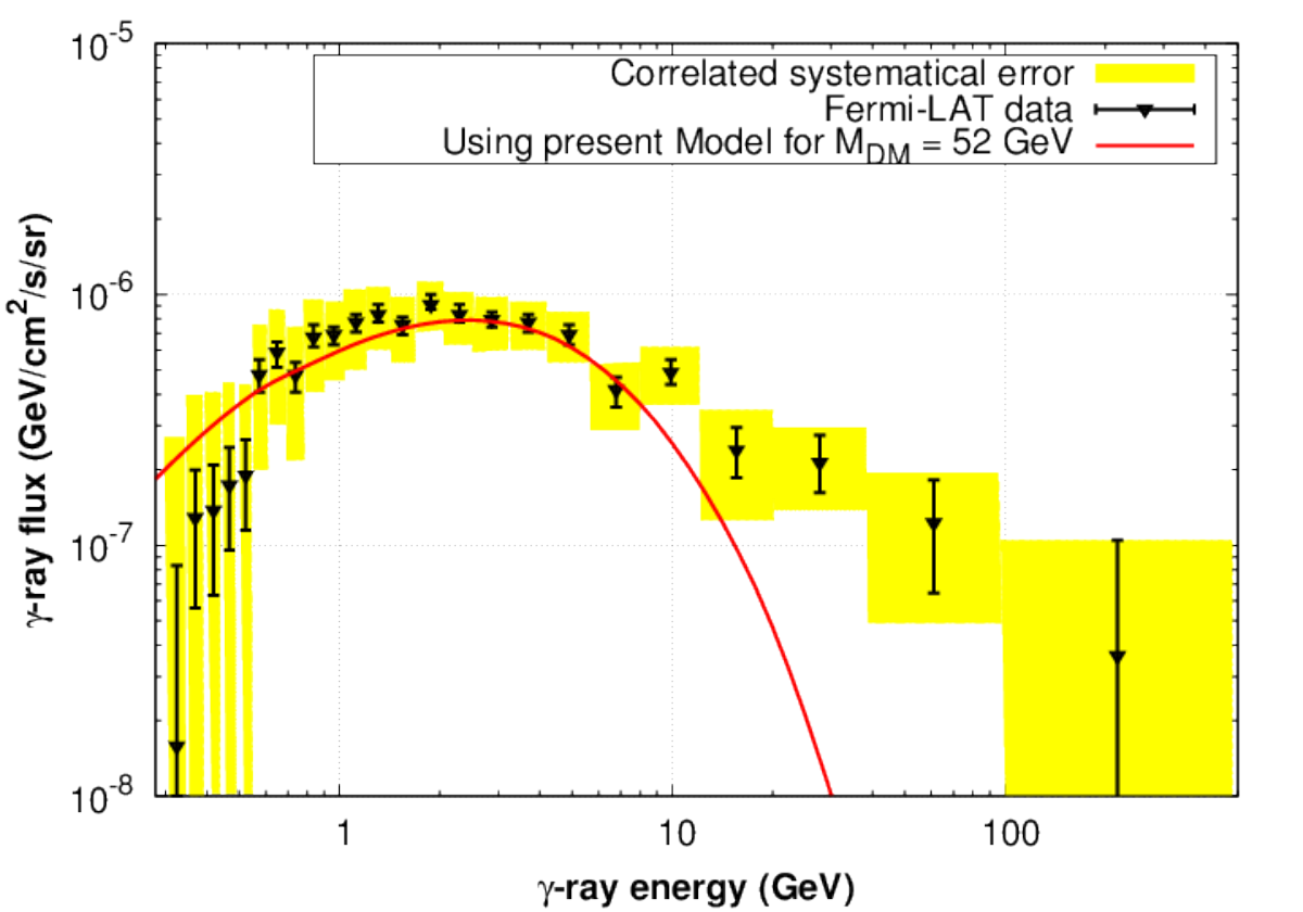
Three allowed values of that we have obtained from the present model for GeV, which are also satisfying all the constrains listed in Section II, are given in Table 3.
|
|
|
|
|
|
|
VI Summary and Conclusion
Existence of neutrino masses and dark matter in the Universe are two of the main observational evidences for physics beyond the Standard Model. If the Galactic Centre gamma ray excess reported by the Fermi-LAT data is indeed due to DM annihilation, then we need our beyond SM physics to be able to explain this excess along with the observed DM relic density as well as neutrino masses and mixing. In this work we showed that the gauged extension of the Standard Model, which can very naturally explain lepton number violation and hence the existence of small Majorana neutrino masses, can also be extended to explain the relic DM density and the Fermi-LAT gamma ray excess, without conflicting with any existing theoretical or observational constraint.
Since symmetry that we impose is local, there is an additional gauge boson in this model. Three right handed neutrinos also have to included in the model to make it anomaly free. In order to break the symmetry spontaneously, one introduces an extra SM singlet scalar which carries a nontrivial charge. The charge of this scalar can be arranged in such a way that the right handed neutrinos pick up Majorana masses when gets a VEV, breaking the symmetry spontaneously. As a result the gauge boson also becomes massive. This extra neutral gauge boson has been searched for at collider experiments which put a stringent bound on the combination of the new gauge coupling and the mass of . We extended this gauged model further by adding another complex SM scalar which is charged under and arranged its charge in such away that all decays of are forbidden making it a stable DM candidate.
We next studied the viability of this model in simultaneously explaining the relic DM density of the Universe as well as the GC gamma ray excess through the annihilation of and into the channel, mediated by , and , where and are the two neutral scalars in our model, of which we identified as the SM-like Higgs with its mass fixed at 125.5 GeV. There are 12 unknown new parameters in this model. We imposed constraints coming from vacuum stability, LEP bound on , LHC bounds on signal strength of the SM-like Higgs and invisible decay width of the SM-like Higgs, and found the regions of the model parameter space which can simultaneously explain the observed DM relic density as well as the Fermi-LAT GC gamma ray excess and at the same time evaded the bounds from the direct detection experiments such as LUX. We showed that for DM masses in the range 40-55 GeV and for a wide range of gauge boson masses, one can satisfy all these constraints if the additional neutral Higgs scalar has a mass around the resonance region. We presented allowed areas in the model parameter space consistent with all relevant data, calculated the predicted gamma ray flux from the GC and discussed the related phenomenology.
In conclusion, the observation of neutrino masses and dark matter are the two main observational evidences of physics beyond the Standard Model. The small neutrino masses can be explained in terms of lepton number violation and the gauged extension of the Standard Model can very easily accommodate the type-I seesaw mechanism since it must have three additional right-handed neutrinos for anomaly cancellation and light Majorana neutrino masses are generated through this seesaw mechanism when the is broken spontaneously. We propose an extension of this model by adding a complex scalar field that acts as the dark matter candidate and make it stable by arranging suitably its charge. We showed that both the relic abundance and the Galactic Centre gamma ray excess could be explained in this model. Thus this model can simultaneously explain neutrino masses, the dark matter relic density of the Universe and the GC gamma ray excess, while simultaneously satisfying all other collider and direct detection constraints. This model should be testable at the next-generation XENON1T experiment.
Acknowledgment
SK wishes to thank N. Chakrabarty and A. Gupta for discussions and S. Kadge and M. Masud for help with numerical codes. The authors would like to thank the Neutrino Project under the XII plan of Harish-Chandra Research Institute. SK and AB also acknowledge the cluster computing facility at HRI (http://cluster.hri.res.in). This project has received funding from the European Union’s Horizon 2020 research and innovation programme under the Marie Sklodowska-Curie grant agreement No 674896.
References
- [1] Y. Sofue and V. Rubin, “Rotation curves of spiral galaxies”, Ann. Rev. Astron. Astrophys. 39, 137 (2001) [astro-ph/0010594].
- [2] M. Bartelmann and P. Schneider, “Weak gravitational lensing”, Phys. Rept. 340, 291 (2001) [astro-ph/9912508].
- [3] D. Clowe, A. Gonzalez and M. Markevitch, “Weak lensing mass reconstruction of the interacting cluster 1E0657-558: Direct evidence for the existence of dark matter”, Astrophys. J. 604, 596 (2004) [astro-ph/0312273].
- [4] G. Hinshaw et al. [WMAP Collaboration], “Nine-Year Wilkinson Microwave Anisotropy Probe (WMAP) Observations: Cosmological Parameter Results”, Astrophys. J. Suppl. 208, 19 (2013) [arXiv:1212.5226 [astro-ph.CO]].
- [5] P. A. R. Ade et al. [Planck Collaboration], “Planck 2015 results. XIII. Cosmological parameters”, arXiv:1502.01589 [astro-ph.CO].
- [6] G. Jungman, M. Kamionkowski and K. Griest, “Supersymmetric dark matter”, Phys. Rept. 267, 195 (1996) [hep-ph/9506380].
- [7] G. Bertone, D. Hooper and J. Silk, “Particle dark matter: Evidence, candidates and constraints”, Phys. Rept. 405, 279 (2005) [hep-ph/0404175].
- [8] J. McDonald, “Gauge singlet scalars as cold dark matter”, Phys. Rev. D 50, 3637 (1994) [hep-ph/0702143 [HEP-PH]].
- [9] C. P. Burgess, M. Pospelov and T. ter Veldhuis, “The Minimal model of nonbaryonic dark matter: A Singlet scalar” Nucl. Phys. B 619, 709 (2001) [hep-ph/0011335].
- [10] A. Biswas and D. Majumdar, “The Real Gauge Singlet Scalar Extension of Standard Model: A Possible Candidate of Cold Dark Matter”, Pramana 80, 539 (2013) [arXiv:1102.3024 [hep-ph]].
- [11] R. Barbieri, L. J. Hall and V. S. Rychkov, “Improved naturalness with a heavy Higgs: An Alternative road to LHC physics”, Phys. Rev. D 74, 015007 (2006) [hep-ph/0603188].
- [12] L. Lopez Honorez, E. Nezri, J. F. Oliver and M. H. G. Tytgat, “The Inert Doublet Model: An Archetype for Dark Matter”, JCAP 0702, 028 (2007) [hep-ph/0612275].
- [13] Y. G. Kim, K. Y. Lee and S. Shin, “Singlet fermionic dark matter” JHEP 0805, 100 (2008) [arXiv:0803.2932 [hep-ph]].
- [14] Y. G. Kim, K. Y. Lee, C. B. Park and S. Shin, “Secluded singlet fermionic dark matter driven by the Fermi gamma-ray excess”, Phys. Rev. D 93, no. 7, 075023 (2016) [arXiv:1601.05089 [hep-ph]].
- [15] T. Hambye, “Hidden vector dark matter”, JHEP 0901, 028 (2009) [arXiv:0811.0172 [hep-ph]].
- [16] O. Lebedev, H. M. Lee and Y. Mambrini, “Vector Higgs-portal dark matter and the invisible Higgs”, Phys. Lett. B 707, 570 (2012) [arXiv:1111.4482 [hep-ph]].
- [17] Q. H. Cao, E. Ma, J. Wudka and C.-P. Yuan, “Multipartite dark matter”, arXiv:0711.3881 [hep-ph].
- [18] K. M. Zurek, “Multi-Component Dark Matter”, Phys. Rev. D 79, 115002 (2009) [arXiv:0811.4429 [hep-ph]].
- [19] G. Belanger and J. C. Park, “Assisted freeze-out” JCAP 1203, 038 (2012) [arXiv:1112.4491 [hep-ph]].
- [20] A. Biswas, D. Majumdar, A. Sil and P. Bhattacharjee, “Two Component Dark Matter : A Possible Explanation of 130 GeV Ray Line from the Galactic Centre”, JCAP 1312, 049 (2013) [arXiv:1301.3668 [hep-ph]].
- [21] L. Bian, R. Ding and B. Zhu, “Two Component Higgs-Portal Dark Matter”, Phys. Lett. B 728, 105 (2014) [arXiv:1308.3851 [hep-ph]].
- [22] S. Bhattacharya, A. Drozd, B. Grzadkowski and J. Wudka, “Two-Component Dark Matter”, JHEP 1310, 158 (2013) [arXiv:1309.2986 [hep-ph]].
- [23] P. Gondolo and G. Gelmini, “Cosmic abundances of stable particles: Improved analysis”, Nucl. Phys. B 360, 145 (1991).
- [24] M. Srednicki, R. Watkins and K. A. Olive, “Calculations of Relic Densities in the Early Universe”, Nucl. Phys. B 310, 693 (1988).
- [25] D. S. Akerib et al. [LUX Collaboration], “First results from the LUX dark matter experiment at the Sanford Underground Research Facility”, Phys. Rev. Lett. 112, 091303 (2014) [arXiv:1310.8214 [astro-ph.CO]].
- [26] D. S. Akerib et al. [LUX Collaboration], “Improved Limits on Scattering of Weakly Interacting Massive Particles from Reanalysis of 2013 LUX Data”, Phys. Rev. Lett. 116, no. 16, 161301 (2016) [arXiv:1512.03506 [astro-ph.CO]].
- [27] E. Aprile et al. [XENON Collaboration], “Physics reach of the XENON1T dark matter experiment”, JCAP 1604, no. 04, 027 (2016) [arXiv:1512.07501 [physics.ins-det]].
- [28] R. Agnese et al. [SuperCDMS Collaboration], “Search for Low-Mass Weakly Interacting Massive Particles with SuperCDMS”, Phys. Rev. Lett. 112, no. 24, 241302 (2014) [arXiv:1402.7137 [hep-ex]].
- [29] D. Hooper, “Particle Dark Matter”, arXiv:0901.4090 [hep-ph].
- [30] L. Goodenough and D. Hooper, “Possible Evidence For Dark Matter Annihilation In The Inner Milky Way From The Fermi Gamma Ray Space Telescope”, [arXiv:0910.2998 [hep-ph]].
- [31] D. Hooper and L. Goodenough, “Dark Matter Annihilation in The Galactic Center As Seen by the Fermi Gamma Ray Space Telescope”, Phys.Lett. B697 (2011) 412–428 [arXiv:1010.2752 [hep-ph]].
- [32] A. Boyarsky, D. Malyshev, and O. Ruchayskiy, “A comment on the emission from the Galactic Center as seen by the Fermi telescope”, Phys.Lett. B705 (2011) 165–169 [arXiv:1012.5839 [hep-ph]].
- [33] D. Hooper and T. Linden, “On The Origin Of The Gamma Rays From The Galactic Center”, Phys.Rev. D84 (2011) 123005 [arXiv:1110.0006 [astro-ph.HE]].
- [34] K. N. Abazajian and M. Kaplinghat, “Detection of a Gamma-Ray Source in the Galactic Center Consistent with Extended Emission from Dark Matter Annihilation and Concentrated Astrophysical Emission”, Phys.Rev. D86 (2012) 083511 [arXiv:1207.6047 [astro-ph.HE]].
- [35] D. Hooper and T. R. Slatyer, “Two Emission Mechanisms in the Fermi Bubbles: A Possible Signal of Annihilating Dark Matter”, Phys.Dark Univ. 2 (2013) 118–138 [arXiv:1302.6589 [astro-ph.HE]].
- [36] K. N. Abazajian, N. Canac, S. Horiuchi, and M. Kaplinghat, “Astrophysical and Dark Matter Interpretations of Extended Gamma-Ray Emission from the Galactic Center”, Phys.Rev. D90 (2014) 023526 [arXiv:1402.4090 [astro-ph.HE]].
- [37] T. Daylan, D. P. Finkbeiner, D. Hooper, T. Linden, S. K. N. Portillo, N. L. Rodd and T. R. Slatyer, “The characterization of the gamma-ray signal from the central Milky Way: A case for annihilating dark matter”, Phys. Dark Univ. 12, 1 (2016) [arXiv:1402.6703 [astro-ph.HE]].
- [38] M. Ajello et al. [Fermi-LAT Collaboration], “Fermi-LAT Observations of High-Energy -Ray Emission Toward the Galactic Center”, Astrophys. J. 819, no. 1, 44 (2016) [arXiv:1511.02938 [astro-ph.HE]].
- [39] P. Agrawal, B. Batell, P. J. Fox and R. Harnik, “WIMPs at the Galactic Center”, JCAP 1505, 011 (2015) [arXiv:1411.2592 [hep-ph]].
- [40] F. Calore, I. Cholis, C. McCabe and C. Weniger, “A Tale of Tails: Dark Matter Interpretations of the Fermi GeV Excess in Light of Background Model Systematics”, Phys. Rev. D 91, no. 6, 063003 (2015) [arXiv:1411.4647 [hep-ph]]. [41]
- [41] W. B. Atwood et al. [Fermi-LAT Collaboration], “The Large Area Telescope on the Fermi Gamma-ray Space Telescope Mission”, Astrophys. J. 697, 1071 (2009) [arXiv:0902.1089 [astro-ph.IM]].
- [42] S. K. Lee, M. Lisanti, B. R. Safdi, T. R. Slatyer and W. Xue, “Evidence for Unresolved -Ray Point Sources in the Inner Galaxy”, Phys. Rev. Lett. 116, no. 5, 051103 (2016) [arXiv:1506.05124 [astro-ph.HE]].
- [43] R. Bartels, S. Krishnamurthy and C. Weniger, “Strong support for the millisecond pulsar origin of the Galactic center GeV excess”, Phys. Rev. Lett. 116, no. 5, 051102 (2016) [arXiv:1506.05104 [astro-ph.HE]].
- [44] J. F. Navarro, C. S. Frenk and S. D. M. White, “A Universal density profile from hierarchical clustering”, Astrophys. J. 490, 493 (1997) [astro-ph/9611107].
- [45] M. S. Boucenna and S. Profumo, “Direct and Indirect Singlet Scalar Dark Matter Detection in the Lepton-Specific two-Higgs-doublet Model”, Phys. Rev. D 84, 055011 (2011) [arXiv:1106.3368 [hep-ph]].
- [46] J. D. Ruiz-Alvarez, C. A. de S.Pires, F. S. Queiroz, D. Restrepo and P. S. Rodrigues da Silva, “On the Connection of Gamma-Rays, Dark Matter and Higgs Searches at LHC”, Phys. Rev. D 86, 075011 (2012) [arXiv:1206.5779 [hep-ph]].
- [47] N. Okada and O. Seto, Phys. Rev. D 89, no. 4, 043525 (2014) doi:10.1103/PhysRevD.89.043525 [arXiv:1310.5991 [hep-ph]].
- [48] A. Alves, S. Profumo, F. S. Queiroz and W. Shepherd, “Effective field theory approach to the Galactic Center gamma-ray excess”, Phys. Rev. D 90, no. 11, 115003 (2014) [arXiv:1403.5027 [hep-ph]].
- [49] A. Berlin, D. Hooper and S. D. McDermott, “Simplified Dark Matter Models for the Galactic Center Gamma-Ray Excess”, Phys. Rev. D 89, 115022 (2014) [arXiv:1404.0022 [hep-ph]].
- [50] P. Agrawal, B. Batell, D. Hooper and T. Lin, “Flavored Dark Matter and the Galactic Center Gamma-Ray Excess”, Phys. Rev. D 90, 063512 (2014) [arXiv:1404.1373 [hep-ph]].
- [51] E. Izaguirre, G. Krnjaic and B. Shuve, “The Galactic Center Excess from the Bottom Up”, Phys. Rev. D 90, 055002 (2014) [arXiv:1404.2018 [hep-ph]].
- [52] D. G. Cerdeño, M. Peiró and S. Robles, “Low-mass right-handed sneutrino dark matter: SuperCDMS and LUX constraints and the Galactic Centre gamma-ray excess”, JCAP 1408, 005 (2014) [arXiv:1404.2572 [hep-ph]].
- [53] S. Ipek, D. McKeen and A. E. Nelson, “A Renormalizable Model for the Galactic Center Gamma Ray Excess from Dark Matter Annihilation”, Phys. Rev. D 90, 055021 (2014) [arXiv:1404.3716 [hep-ph]].
- [54] C. Boehm, M. J. Dolan and C. McCabe, “A weighty interpretation of the Galactic Centre excess”, Phys. Rev. D 90, 023531 (2014) [arXiv:1404.4977 [hep-ph]].
- [55] P. Ko, W. I. Park and Y. Tang, “Higgs portal vector dark matter for scale -ray excess from galactic center”, JCAP 1409, 013 (2014) [arXiv:1404.5257 [hep-ph]].
- [56] M. Abdullah, A. DiFranzo, A. Rajaraman, T. M. P. Tait, P. Tanedo and A. M. Wijangco, “Hidden on-shell mediators for the Galactic Center -ray excess”, Phys. Rev. D 90, no. 3, 035004 (2014) [arXiv:1404.6528 [hep-ph]].
- [57] D. K. Ghosh, S. Mondal and I. Saha, “Confronting the Galactic Center Gamma Ray Excess With a Light Scalar Dark Matter”, JCAP 1502, no. 02, 035 (2015) [arXiv:1405.0206 [hep-ph]].
- [58] A. Martin, J. Shelton and J. Unwin, “Fitting the Galactic Center Gamma-Ray Excess with Cascade Annihilations”, Phys. Rev. D 90, no. 10, 103513 (2014) [arXiv:1405.0272 [hep-ph]].
- [59] L. Wang and X. F. Han, “A simplified 2HDM with a scalar dark matter and the galactic center gamma-ray excess”, Phys. Lett. B 739, 416 (2014) [arXiv:1406.3598 [hep-ph]].
- [60] T. Mondal and T. Basak, “Class of Higgs-portal Dark Matter models in the light of gamma-ray excess from Galactic center”, Phys. Lett. B 744, 208 (2015) [arXiv:1405.4877 [hep-ph]].
- [61] W. Detmold, M. McCullough and A. Pochinsky, “Dark Nuclei I: Cosmology and Indirect Detection”, Phys. Rev. D 90, 115013 (2014) [arXiv:1406.2276 [hep-ph]].
- [62] C. Arina, E. Del Nobile and P. Panci, “Dark Matter with Pseudoscalar-Mediated Interactions Explains the DAMA Signal and the Galactic Center Excess”, Phys. Rev. Lett. 114, 011301 (2015) [arXiv:1406.5542 [hep-ph]].
- [63] N. Okada and O. Seto, “Galactic Center gamma-ray excess from two-Higgs-doublet-portal dark matter”, Phys. Rev. D 90, no. 8, 083523 (2014) [arXiv:1408.2583 [hep-ph]].
- [64] K. Ghorbani, “Fermionic dark matter with pseudo-scalar Yukawa interaction”, JCAP 1501, 015 (2015) [arXiv:1408.4929 [hep-ph]].
- [65] A. D. Banik and D. Majumdar, “Low Energy Gamma Ray Excess Confronting a Singlet Scalar Extended Inert Doublet Dark Matter Model”, Phys. Lett. B 743, 420 (2015) [arXiv:1408.5795 [hep-ph]].
- [66] A. Biswas, “Explaining Low Energy -ray Excess from the Galactic Centre using a Two Component Dark Matter Model”, J. Phys. G 43, no. 5, 055201 (2016) [arXiv:1412.1663 [hep-ph]].
- [67] K. Ghorbani and H. Ghorbani, “Scalar split WIMPs in future direct detection experiments”, Phys. Rev. D 93, no. 5, 055012 (2016) [arXiv:1501.00206 [hep-ph]].
- [68] D. G. Cerdeno, M. Peiro and S. Robles, “Fits to the Fermi-LAT GeV excess with RH sneutrino dark matter: implications for direct and indirect dark matter searches and the LHC”, Phys. Rev. D 91, no. 12, 123530 (2015) [arXiv:1501.01296 [hep-ph]].
- [69] A. Biswas, D. Majumdar and P. Roy, “Nonthermal two component dark matter model for Fermi-LAT -ray excess and 3.55 keV X-ray line”, JHEP 1504, 065 (2015) [arXiv:1501.02666 [hep-ph]].
- [70] A. Achterberg, S. Amoroso, S. Caron, L. Hendriks, R. Ruiz de Austri and C. Weniger, “A description of the Galactic Center excess in the Minimal Supersymmetric Standard Model”, JCAP 1508, no. 08, 006 (2015) [arXiv:1502.05703 [hep-ph]].
- [71] D. Borah, A. Dasgupta and R. Adhikari, “Common origin of the 3.55 keV x-ray line and the Galactic Center gamma-ray excess in a radiative neutrino mass model”, Phys. Rev. D 92, no. 7, 075005 (2015) [arXiv:1503.06130 [hep-ph]].
- [72] A. D. Banik, D. Majumdar and A. Biswas, “Possible Explanation of Indirect Gamma Ray Signatures from Hidden Sector SU(2)H Fermionic Dark Matter”, arXiv:1506.05665 [hep-ph].
- [73] B. Dutta, Y. Gao, T. Ghosh and L. E. Strigari, “Confronting Galactic center and dwarf spheroidal gamma-ray observations with cascade annihilation models”, Phys. Rev. D 92, no. 7, 075019 (2015) [arXiv:1508.05989 [hep-ph]].
- [74] A. Cuoco, B. Eiteneuer, J. Heisig and M. Krämer, “A global fit of the -ray galactic center excess within the scalar singlet Higgs portal model”, arXiv:1603.08228 [hep-ph].
- [75] R. N. Mohapatra and R. E. Marshak, “Local B-L Symmetry of Electroweak Interactions, Majorana Neutrinos and Neutron Oscillations”, Phys. Rev. Lett. 44, 1316 (1980) Erratum: [Phys. Rev. Lett. 44, 1643 (1980)].
- [76] H. M. Georgi, S. L. Glashow and S. Nussinov, “Unconventional Model of Neutrino Masses”, Nucl. Phys. B 193, 297 (1981).
- [77] C. Wetterich, “Neutrino Masses and the Scale of B-L Violation”, Nucl. Phys. B 187, 343 (1981).
- [78] M. Lindner, D. Schmidt and T. Schwetz, “Dark Matter and neutrino masses from global U(1)B-L symmetry breaking”, Phys. Lett. B 705, 324 (2011) [arXiv:1105.4626 [hep-ph]].
- [79] N. Okada and O. Seto, “Higgs portal dark matter in the minimal gauged model”, Phys. Rev. D 82, 023507 (2010) [arXiv:1002.2525 [hep-ph]].
- [80] N. Okada and Y. Orikasa, “Dark matter in the classically conformal B-L model”, Phys. Rev. D 85, 115006 (2012) [arXiv:1202.1405 [hep-ph]].
- [81] L. Basso, O. Fischer and J. J. van der Bij, “Natural Z′ model with an inverse seesaw mechanism and leptonic dark matter”, Phys. Rev. D 87, no. 3, 035015 (2013) [arXiv:1207.3250 [hep-ph]].
- [82] T. Basak and T. Mondal, “Constraining Minimal model from Dark Matter Observations”, Phys. Rev. D 89, 063527 (2014) [arXiv:1308.0023 [hep-ph]].
- [83] B. L. Sánchez-Vega, J. C. Montero and E. R. Schmitz, “Complex Scalar DM in a B-L Model”, Phys. Rev. D 90, no. 5, 055022 (2014) [arXiv:1404.5973 [hep-ph]].
- [84] J. Guo, Z. Kang, P. Ko and Y. Orikasa, “Accidental dark matter: Case in the scale invariant local B-L model”, Phys. Rev. D 91, no. 11, 115017 (2015) [arXiv:1502.00508 [hep-ph]].
- [85] W. Rodejohann and C. E. Yaguna, “Scalar dark matter in the model”, JCAP 1512, no. 12, 032 (2015) [arXiv:1509.04036 [hep-ph]].
- [86] N. Okada and S. Okada, “ portal dark matter and LHC Run-2 results”, Phys. Rev. D 93, no. 7, 075003 (2016) [arXiv:1601.07526 [hep-ph]].
- [87] W. Buchmuller and T. Yanagida, “Baryogenesis and the scale of B-L breaking”, Phys. Lett. B 302, 240 (1993).
- [88] W. Buchmuller and M. Plumacher, “Baryon asymmetry and neutrino mixing”, Phys. Lett. B 389, 73 (1996) [hep-ph/9608308].
- [89] T. R. Dulaney, P. Fileviez Perez and M. B. Wise, “Dark Matter, Baryon Asymmetry, and Spontaneous B and L Breaking”, Phys. Rev. D 83, 023520 (2011) [arXiv:1005.0617 [hep-ph]].
- [90] M. Carena, A. Daleo, B. A. Dobrescu and T. M. P. Tait, “ gauge bosons at the Tevatron”, Phys. Rev. D 70, 093009 (2004) [hep-ph/0408098].
- [91] G. Cacciapaglia, C. Csaki, G. Marandella and A. Strumia, “The Minimal Set of Electroweak Precision Parameters”, Phys. Rev. D 74, 033011 (2006) [hep-ph/0604111].
- [92] G. Aad et al. [ATLAS Collaboration], Phys. Rev. D 90, no. 5, 052005 (2014) doi:10.1103/PhysRevD.90.052005 [arXiv:1405.4123 [hep-ex]].
- [93] J. M. Cline, K. Kainulainen, P. Scott and C. Weniger, “Update on scalar singlet dark matter”, Phys. Rev. D 88, 055025 (2013) Erratum: [Phys. Rev. D 92, no. 3, 039906 (2015)] [arXiv:1306.4710 [hep-ph]].
- [94] G. Belanger, F. Boudjema, A. Pukhov and A. Semenov, “Dark matter direct detection rate in a generic model with micrOMEGAs 2.2”, Comput. Phys. Commun. 180, 747 (2009) [arXiv:0803.2360 [hep-ph]].
- [95] K. A. Olive et al. [Particle Data Group Collaboration], “Review of Particle Physics”, Chin. Phys. C 38, 090001 (2014).
- [96] P. Bechtle, S. Heinemeyer, O. Stål, T. Stefaniak and G. Weiglein, “Probing the Standard Model with Higgs signal rates from the Tevatron, the LHC and a future ILC”, JHEP 1411, 039 (2014) [arXiv:1403.1582 [hep-ph]].
- [97] G. Belanger, B. Dumont, U. Ellwanger, J. F. Gunion and S. Kraml, “Status of invisible Higgs decays”, Phys. Lett. B 723, 340 (2013) [arXiv:1302.5694 [hep-ph]].
- [98] J. Edsjo and P. Gondolo, “Neutralino relic density including coannihilations”, Phys. Rev. D 56, 1879 (1997) [hep-ph/9704361].
- [99] G. Belanger, F. Boudjema, A. Pukhov and A. Semenov, “micrOMEGAs-3: A program for calculating dark matter observables”, Comput. Phys. Commun. 185, 960 (2014) [arXiv:1305.0237 [hep-ph]].
- [100] A. Semenov, “LanHEP - a package for automatic generation of Feynman rules from the Lagrangian. Updated version 3.1”, arXiv:1005.1909 [hep-ph].
- [101] M. Cirelli et al., “PPPC 4 DM ID: A Poor Particle Physicist Cookbook for Dark Matter Indirect Detection”, JCAP 1103, 051 (2011) Erratum: [JCAP 1210, E01 (2012)] [arXiv:1012.4515 [hep-ph]].
- [102] J. Einasto, “On the construction of a composite model for the galaxy and on the determination of the system of galactic parameters”, Trudy Inst. Astrofiz. Alma-Ata 5 87 (1965).
- [103] L. Bergstrom, P. Ullio and J. H. Buckley, “Observability of gamma-rays from dark matter neutralino annihilations in the Milky Way halo”, Astropart. Phys. 9, 137 (1998) [astro-ph/9712318].
- [104] B. Moore, T. R. Quinn, F. Governato, J. Stadel and G. Lake, “Cold collapse and the core catastrophe”, Mon. Not. Roy. Astron. Soc. 310, 1147 (1999) [astro-ph/9903164].