Thermodynamics of the two-dimensional XY model from functional renormalization
Abstract
We solve the nonperturbative renormalization-group flow equations for the two-dimensional XY model at the truncation level of the (complete) second-order derivative expansion. We compute the thermodynamic properties in the high-temperature phase and compare the non-universal features specific to the XY model with results from Monte Carlo simulations. In particular, we study the position and magnitude of the specific heat peak as a function of temperature. The obtained results compare well with Monte Carlo simulations. We additionally gauge the accuracy of simplified nonperturbative renormalization-group treatments relying on -type truncations. Our computation indicates that such an approximation is insufficient in the high- phase and a correct analysis of the specific heat profile requires account of an infinite number of interaction vertices.
I Introduction
It has since long been recognized [1, 2, 3, 4, 5] that the two-dimensional XY model undergoes a Kosterlitz-Thouless (KT) phase transition upon varying temperature . This transition is peculiar in a number of respects: it is not accompanied by the appearance of long-range order (which is prohibited by the Mermin-Wagner theorem [6]) and the free energy is a smooth ( class) function of the thermodynamic parameters. Nonetheless, the low- phase displays long-range correlations and order-parameter stiffness. The latter exhibits a universal jump upon crossing the transition temperature . The correlation length is characterized by an essential singularity in the vicinity of the transition in the high- phase. A distinct nonuniversal feature of the model is the pronounced, asymmetric peak of the specific heat as a function of . The occurrence of this maximum is usually attributed to a rapid increase of entropy upon unbinding the vortex-antivortex pairs. The peak is located somewhat above the transition temperature . It is peculiar that on one hand the maximum is well separated from the asymptotic critical region, and, on the other, it occurs in a temperature range where the correlation length is still very large compared to the microscopic scale.
The Kosterlitz-Thouless transition is relevant in a number of physical contexts [7] such as magnetism, liquid crystals, melting of two-dimensional () solids, superfluidity and superconductivity. Experimentally the KT-type behavior was observed in liquid-helium films [8, 9, 10] and atomic gases [11, 12, 13, 14].
The universal aspects of the KT transition are conventionally described in the language of vortex-antivortex pair unbinding and a mapping to a Coulomb gas or sine-Gordon field theory. The predictivity of such formulations is typically restricted to the behavior in the vicinity of the transition, which makes it harder to access the non-universal, system specific properties, such as the critical temperature or the position, magnitude and width of the specific-heat peak.
In the present work we develop and extend the description of the KT transition using the non-perturbative renormalization group (RG). We build upon earlier works [15, 16, 17], which, however, were limited to -type effective models and focused exclusively on universal aspects of the transition. The formulation evades the explicit introduction of vortices as degrees of freedom, and, in the form presented here, takes a microscopic spin system as the starting point. On the other hand, the approach captures the low-wavelength infrared (IR) asymptotics and respects the Mermin-Wagner theorem. In the present analysis we focus primarily on the relatively simple XY model on a square lattice, where the results obtained at different approximation levels of the RG framework can be compared to ample Monte Carlo (MC) data [18, 19, 20, 21, 22, 23, 24, 25]. Observe however that the verification of the theoretical predictions of the KT theory by MC simulations has not always been conclusive even with respect to the most basic properties. For a critical discussion of these issues see Ref. [22]. The present approach complements the MC in that it is formulated directly for infinite volume and does not invoke finite-size scaling theory. It also differs from the standard RG treatments in evading introduction of vortices or any expansions in powers of the order-parameter field. We show that the latter is crucial for a correct (even qualitatively) account of thermodynamics in the high- phase.
The nonperturbative RG is among the methods allowing for accurate computations of critical behavior in diverse systems. Its applicability is in addition by no means restricted to the vicinity of a phase transition. It has proven useful in a wide range of complex physical contexts. Examples include models with competing orders [26, 27, 28, 29] or situations out of equilibrium [30, 31, 32]. The formalism by itself sheds light on fundamental aspects of critical phenomena (see e.g. [33, 34]), leading to a genuine progress of the field. On the other hand, not so often do the computations within this approach reach high-precision accuracy away from the critical region. The precise predictions also typically depend somewhat on the choice of regularization. Ref. [35] shows that the critical temperature of the 3-dimensional Ising model may be calculated with the accuracy of around 1%. Going beyond this precision level would require a substantial effort. The presently analyzed case of the 2-dimensional XY model is methodologically very distinct for at least two reasons: (1) The physics governing the vicinity of the phase transition is dominated by the anomalous dimension (which is negligible in for most purposes); (2) fluctuation effects are stronger (and lead to ultimate obliteration of long-range order) due to the presence of the Goldstone mode.
Our framework automatically encodes the Mermin-Wagner theorem and is (upon slight modifications) extendable to more complex systems characterized by similar low-energy behavior at finite temperatures. These include quantum spins as well as interacting bosons or fermions in . Such systems were already studied within simpler nonperturbative RG truncations, see e.g. [36, 37, 38, 39, 40, 41]. However, the latter are not sufficient to correctly account for nonuniversal features related to the KT transition - see Sec. V. Before embarking on the more complex problems mentioned above, it is important to understand the merits and limitations of the method in situations where the results can be reliably compared to other approaches.
II The XY model and the corresponding lattice field theory
The classical XY model on a lattice is defined by the Hamiltonian
| (1) |
where label the sites of the lattice, , , and the summation is implicit wherever the index appears exactly twice in a product expression.
The corresponding partition function is given by
| (2) |
Here and denotes the angle between the vector and the -axis, so that and for each .
In order to cast the problem of evaluating the partition function in the language of field theory, we employ the identity
| (3) |
where the normalization factor is given by
| (4) |
Here is a two-dimensional vector attributed to the lattice site . Eq. (3) applies provided the matrix is positive-definite. The non-positivity can be cured by shifting the matrix by a constant diagonal term, which, in our setup, amounts to transforming the Hamiltonian Eq. (1) via
| (5) |
i.e. shifting it by a constant equal . Specifying
| (6) |
we apply Eq. (3) to Eq. (2). The resulting expression for the partition function still involves the multiple integration over the spin variables , which can now be explicitly performed
| (7) |
Here denotes the hyperbolic Bessel function of first kind. This way we cast the partition function in the form
| (8) |
In order to make all the temperature dependencies explicit, we rescale the interaction matrix and the fluctuating field according to:
| (9) |
This way the partition function becomes expressed as
| (10) |
with
| (11) |
and
| (12) |
Importantly, the change of variables of Eq. (9) removes temperature dependencies from the integration measure as well as the kinetic term in the effective action , and absorbs it fully into the local potential term . This aspect is crucial for the validity of the subsequent approximate RG procedure of Sec. III and IV. The choice introduced in Eq. (9) differs from some standard conventions [42].
Eq.(10-12) define the starting point for our computations. Specific lattice and interaction types may now be addressed by specifying the corresponding matrix . Assuming translational invariance the kinetic term in is diagonalized with the Fourier transform:
| (13) |
where
| (14) |
This establishes the explicit form of the kinetic term.
II.1 Mean-field theory for ferromagnetic order
Assuming a form of favoring ferromagnetic ordering, one identifies the mean-field free energy as the minimum of . Restricting to uniform field configurations the mean-field equilibrium value of is given by
| (15) |
The mean-field critical temperature is obtained by expanding the above around up to terms linear in . This relates the critical temperature to :
| (16) |
The corresponding critical exponents are classical and the critical temperature of Eq. (16) carries a strong, linear dependence on the parameter [42]. Obviously, the resulting occurrence of long-range order at mean-field level contradicts the Mermin-Wagner theorem. In addition we observe that the mean-field free energy, and, in consequence, also the specific heat is zero in the high-temperature phase.
II.2 Nearest-neighbor interactions
For the square lattice with nearest-neighbor interactions we obtain
| (17) |
where is the nearest-neighbor coupling and denotes the lattice spacing. The latter will be put equal to 1 in all numerical calculations.
III Nonperturbative RG
The central idea of the nonperturbative renormalization group approach to equilibrium condensed-matter systems is to recast the problem of computing the partition function in a form of a (functional) differential equation. There exists a number of variants of this program. The presently applied formulation, developed by Wetterich [43], relies on the concept of a flowing scale-dependent effective action . This quantity continuously connects the microscopic action (in the present work given by Eq. (11)) with the full free energy upon varying the flow parameter . The latter is here taken to be an IR momentum cutoff scale. It serves to add a mass of order to the fluctuation modes, effectively freezing their propagation for momenta . Lowering the cutoff scale implies including modes of progressively lower momenta. For vanishing all fluctuation modes are included into the partition function and we find as . The variation of upon changing is governed by the flow equation [43]:
| (18) |
where denotes the second functional derivative of . In Fourier space, the trace (Tr) sums over momenta and the field index . The quantity is the momentum cutoff function added to the inverse propagator to freeze the fluctuations with momenta . An exact solution of Eq. (18) with the initial condition given by Eq. (11) would imply finding the partition function . This is not achievable, but the framework of Eq. (18) offers a number of approximation schemes [44, 45, 26, 46] going beyond those accessible within the more traditional approaches.
III.1 Derivative expansion
In this work we apply the derivative expansion [44, 46, 47, 48] (DE) in which the symmetry-allowed terms in are classified according to the number of derivatives (or powers of in momentum space). The most general expression at level (or ) reads:
| (19) |
where . We impose restrictions neither on the effective potential nor the gradient functions , , which are allowed to depend on the cutoff scale . The occurrence of two gradient terms is due to the fact that the transverse and radial components of the field are characterized by different stiffness coefficients. We also observe here that the initial condition Eq. (11) contains terms of all powers of . In fact, the initial condition does not quite fit the ansatz of Eq. (19) since the kinetic term involves functions of arbitrarily high order in . We come back to this point later on. Plugging the ansatz of Eq. (19) into Eq. (18) yields a projection of the Wetterich equation onto a set of three coupled non-linear partial differential equations describing the flow of , and , which may be handled numerically. It is advantageous to perform a canonical rescaling of the flowing quantities by defining
| (20) |
where and the factor is conventional. The -dependent constant (wave-function renormalization) is defined by imposing the condition where is an arbitrary renormalization point on the rescaled grid. The scale-dependent anomalous dimension is then given by
| (21) |
and the physical anomalous dimension follows from . We refrain from quoting the lengthy explicit expressions for the flow equations. These are given in Ref. [16] and in the appendix of Ref. [17]. The transition temperature is extracted following Ref. [17] by using the fact that the flowing minimum of the (nonrescaled) effective potential vanishes as in the low- phase. This is consistent with both the absence of the long-range order and algebraic decay of correlations governed by the anomalous dimension . Since for , the minimum of the rescaled potential remains finite for as long as , and vanishes otherwise.
III.2 Initial condition for the propagator
The proposed approach relies on two approximations. First: the flowing effective action is parametrized by the ansatz of Eq. (19). This implies retaining the most general -invariant form of the action but only up to terms of order . In particular the local potential is allowed to contain arbitrarily high powers of . Second: as we already remarked, the initial action of Eq. (11) involves terms of higher order in than . We, however, cast it in a form consistent with Eq. (19) by expanding the dispersion in Eq. (11) around . Physically this may be understood as ”smearing” or coarse-graining the lattice structure ”by hand”. In a somewhat more subtle treatment one might split the flow into two stages. In the initial part () of the flow hardly any renormalization of and occurs, but the cosine dispersion may play a role. In the second stage () the lattice no longer matters.
An interesting alternative is provided by the lattice non-perturbative RG framework [35], where the initial stage of the flow is overall bypassed, and the initial condition is not given by the bare action, but, instead, is computed from the local limit of decoupled sites. This program, however, places restrictions on the cutoff, which are most naturally fulfilled by a non-smooth Litim-type regulator [49]. This in turn renders the flow much less stable numerically. Such complications are most severe in . We observe no signatures of numerical instabilities in our variant of approximation. In addition our calculation requires a significantly smaller field grid than that of Ref. [35].
Our strategy to perform the -expansion from the outset instead of the slightly more accurate treatments mentioned above also stems from the aim to develop a numerically modest and stable framework flexibly extendable to other contexts (such as interacting quantum gases in ). The present approximation allows to avoid any two-dimensional integrations in the flow equations. Also observe that the dominant contributions to all the integrals come from small momenta also for large, and, of course, upon reducing the approximation becomes progressively more accurate. By reasoning a posteriori our results suggest that the error from neglecting the cosine dispersion amounts to a shift of the critical temperature (see Sec. IV).
The second derivative matrix in the propagator at the beginning of the flow thus reads
| (22) |
We extract and from the coefficients of the expansion of around . Here is the initial cutoff scale. In fact, we obtain and . We note that alternative to Eq. (9) rescalings of the fluctuating field and interaction matrix, such as that of Ref. [42], generate both and dependencies in the initial condition.
The momentum integrations in the flow equations are computed over a disc of radius . In a non-approximate treatment they should run over the Brillouin zone ( for a square lattice). The scale is often identified with the scale where the flow is initiated. In fact these quantities are distinct, and, in principle should be taken infinite to assure that all fluctuations are frozen, so that the action Eq. (11) is the correct starting point. In a practical numerical implementation we take and assure that the inverse propagators at high scales are completely dominated by the cutoff term.
III.3 Numerical solution
Numerical integration of the flow equations proceeds along the line of Ref. [17]. There are however two important differences. Ref. [17] used an effective action as a starting point, while here the initial condition follows from Eq. (11) (see below). The other difference is that in the present calculation we extract thermodynamic quantities (specific heat in particular) related directly to the free energy, which is given by . While for the purposes of Ref. [17] it was sufficient to compute the flow of the -derivative of the rescaled potential , here we additionally compute the flow of the (nonrescaled) potential . The corresponding flow equation, supplementing the flow equations given in Ref. [17] reads:
| (23) |
where and the dimensionless -dependent longitudinal and transverse inverse propagators are given by
| (24) |
A reliable calculation demands high numerical accuracy. This is because we solve the flow equations for a set of initial conditions parametrized by temperature and subsequently evaluate the entropy and the specific heat by numerically computing the first two derivatives of the result for the free energy with respect to .
We also observe that, since we explore the high-temperature phase and the vicinity of the phase transition in the low- phase, the principal problem of encountering the pole of the flow equations described in Ref. [17] is irrelevant here.
In the practical numerical solution we employ the smooth Wetterich cutoff
| (25) |
The inclusion of the wave-function renormalization in is a requirement for the possibility of obtaining scale-invariant solutions. The parameter is in principle arbitrary. Ref. [17] rose the question of the existence of exact (functional) fixed points of the flow depending on its value. The present analysis is performed at fixed which is close to the ”optimal” value in the immediate vicinity of the transition. We refer to [17] for an extensive discussion of this issue.
IV Numerical Results
For the nearest-neighbor XY model is given by Eq. (17) and it follows that the initial condition for and reads
| (26) |
while the initial effective potential is given by
| (27) |
We observe that both and depend on the arbitrary parameter . In fact, as we already pointed out, the mean-field transition temperature of Eq. (16) carries a strong -dependence. Adding fluctuations by the non-perturbative RG flow drastically reduces this dependence, but does not remove it completely, as discussed below. Also observe that (at least formally) the above expressions for and make sense for arbitrary non-negative values of . On the other hand, for the present case of nearest-neighbor interactions, the matrix is positive-definite for .
IV.1 Critical temperature
The critical temperature is estimated by following the flow of the minimum of the (rescaled) effective potential. This quantity reaches zero at a finite scale for the system in the high- phase, and attains an (approximate) fixed-point in the KT-phase. Equivalently, one may inspect the evolution of the anomalous exponent , vanishing in the high- phase for sufficiently small and attaining a ”plateau” otherwise. The procedure follows Ref. [17] and is illustrated in Fig. 1 where we plot as a function of . Also note that the method of estimating is different from the MC, which typically employs a fit of the theoretical formulae for the correlation length and susceptibility to the simulation data.

In Ref. [35] only a very weak dependence of the critical temperature on the parameter was found in the case of the Ising model in three dimensions. In the present case we observe a monotonous dependence of the KT temperature on the parameter ranging between for and for . The dependence of on slowly ceases at larger values of . Large values of are however very unpractical because becomes very small. Our estimate of may be compared to the MC results which give . The lattice version of nonperturbative RG yielded the estimate [35].
We believe that the mechanism responsible for the annihilation (or significant reduction) of the -dependence of the critical temperature is related to the fact that even though the position of the minimum of carries a strong -dependence, the minimum of the initial rescaled potential shows only a very weak sensitivity to the variation of . On the other hand, the profile of for does depend on . The dependence of on should be efficiently eliminated by the flow in situations, where the essential features of the flow are captured by the behavior of the effective action around . The mechanism is expected to be less efficient otherwise. This condition is better fulfilled in . Our procedure of performing the -expansion from the beginning is also of relevance for the results for . The dependence of our estimate of on is an unpleasant feature and we perceive it as a deficiency of the present approach. It is possible to choose so that we obtain in precise agreement with MC, but this is not what we aim at. We note however that the -dependence of is by far weaker than at mean-field level. In addition, the thermodynamic quantities discussed below are insensitive to the choice of provided they are computed relative to . This suggests that the error related to our approximation is absorbed by a shift of , leaving other thermodynamic quantities hardly affected.
IV.2 Entropy and specific heat
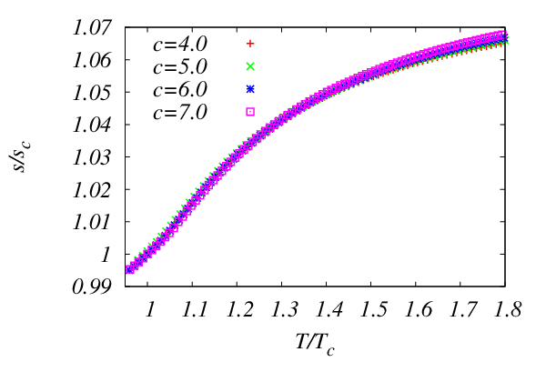
We proceed by evaluating the entropy at zero magnetic moment (or, equivalently, zero magnetic field), which, by elementary thermodynamics follows from . The free energy is obtained from the integrated flow via . It is also possible to extend the analysis to non-zero fields since the magnetic field, the order parameter field and free energy are related by . By computing the flow for different we extract the free energy profiles for a range of temperatures and subsequently evaluate the (discrete) derivative with respect to . The results are shown in Fig. (2). We observe a collapse of the curves computed for different if the variables are scaled by the critical values. The entropy is a positive, monotonously increasing function of temperature, as expected from the principles of thermodynamics. The signatures of the transition are not visible in the -derivatives of the thermodynamic potential (as is expected from the -theory and also consistent with the results of simulations).
In the next step we evaluate the specific heat (at zero magnetization). This is given by
| (28) |
The results obtained for different choices of are plotted in Fig. (3). Again, the dependence on does not occur once we use the reduced variable. The pronounced maximum shows an asymmetry similar to those found in MC. The peak is located around and reaches up to . Both these quantities are close to the MC and tensor RG results. More specifically (see e.g. [18, 23, 25]), the MC peak is located at and reaches up to . Note however, that the free energy plotted in Ref. [25] has positive slope, and the entropy obtained therein is negative. The reasons for this are not clear to us. The level of agreement of and between the MC and tensor RG results reported in [25] is very high.
It is striking that the rich thermodynamic structure described in this section emerged via the functional RG flow from the mean-field free energy, which is trivially equal zero in the high- phase (see Sec. II A).

IV.3 Equation of state
The magnetic field at given is extracted from the definition
| (29) |
which yields the equation of state . The isothermal susceptibility at zero field is given as the derivative
| (30) |
and becomes very large upon lowering temperature towards . The dependence is shown in Fig. 4 for a sequence of temperatures.

V Remarks on the truncation
It is useful to compare the above calculation to a much simpler treatment relying on the -type expansion. It is natural to invoke a largely simplified ansatz for the effective potential
| (31) |
and also restrict and to flowing couplings corresponding to the functions evaluated at the potential minimum (). The problem may then be cast onto a set of five coupled ordinary differential flow equations for the couplings , , , and . The initial condition for the potential is extracted by expanding the effective potential in Eq. (11) around its minimum. The ansatz Eq. (31) makes sense for . Once the flow crosses over into the regime with one switches to the parametrization suitable for the high-temperature phase
| (32) |
The free energy may then be extracted from . In fact, a very similar truncation (neglecting and ) was employed in Ref. [15] and yielded a plausible picture of the KT transition.
We have solved the above mentioned set of flow equations and compared the results to those obtained within the complete derivative expansion in Sec. IV. Even though the estimate of the critical temperature is in a reasonable range, the approximation badly fails for the thermodynamic quantities. In fact the obtained free energy is not a concave function of temperature, yielding, for example, a negative specific heat in a range of temperatures. The reason for this becomes clear after inspecting Eq. (11). Expanding the effective potential in implies uncontrolled dropping of temperature dependencies, which, as turns out, leads to a drastic deformation of the result.
VI Summary and outlook
We have solved the non-perturbative RG flow equations for the two-dimensional XY model at the approximation level of the complete second order derivative expansion. From the obtained free energy we computed the non-universal thermodynamic properties in the the high-temperature phase. Wherever possible, we compared the results to Monte Carlo simulations. We found satisfactory agreement for the entropy and specific heat. In particular, the location and magnitude of the specific heat peak relative to compare very well to MC data. This is one of the few RG-based computations for this quantity in this model. As we pointed out, the specific heat peak occurs in a regime which on one hand is off the asymptotic critical region, and, on the other, is characterized by large correlation length. Such a situation is somewhat atypical. An interesting RG calculation was performed in Ref. [25] within the tensor RG framework, which may be viewed as a reincarnation of the ideas of direct real-space coarse-graining scheme. However, it is not clear to what extent that approach can be generalized to other systems.
Our estimate of the Kosterlitz-Thouless temperature is not far from the correct value, however the present method cannot serve as a high-precision tool in this case. We argue that the location of the transition is the quantity that is most strongly affected by the approximations, in particular by the relatively simple treatment of the dispersion at the initial stages of the flow. As we pointed out, the thermodynamic functions become insensitive to the arbitrary parameter of the Hamiltonian upon scaling by .
We compared the full derivative expansion to a simplified treatment invoking vertex expansion (-type theory), which is commonly applied in different contexts. The latter framework turns out not to be sufficient for computing the non-universal thermodynamic quantities, since it truncates relevant temperature dependencies in the neglected vertices.
The present calculation bridges a microscopic model with macroscopic thermodynamics via the functional flow equation, accounting for the low-energy asymptotics specific to two-dimensional systems with symmetry. It will now be natural and interesting to perform analogous studies of systems characterized by similar infrared physics, including interacting quantum gases in .
Acknowledgements.
We are grateful to Nicolas Dupuis and Walter Metzner for useful discussions. We also thank Walter Metzner for reading the manuscript and a number of valuable remarks. PJ acknowledges funding from the Polish National Science Center via grant 2014/15/B/ST3/02212. AE acknowledges support from the German National Academy of Sciences Leopoldina through grant LPDS 2014-13.References
- [1] V. L. Berezinskii, Sov. Phys. JETP 32, 493 (1970).
- [2] V. L. Berezinskii, Sov. Phys. JETP 34, 610 (1971).
- [3] J. M. Kosterlitz and D. J. Thouless, J. of Phys. C 6, 1181 (1973).
- [4] J. M. Kosterlitz and D. J. Thouless, J. of Phys. V 7, 1046 (1974).
- [5] J. Fröhlich, T. Spencer, Commun. Math. Phys. 81, 527 (1981).
- [6] N. D. Mermin and H. Wagner, Phys. Rev. Lett. 17, 1133 (1966).
- [7] P. M. Chaikin and T. C. Lubensky, Principles of Condensed Matter Physics (Cambridge University Press, 1995).
- [8] D. J. Bishop and J. D. Reppy, Phys. Rev. Lett. 40, 1727 (1978).
- [9] J. Maps and R. B. Hallock, Phys. Rev. Lett. 47, 1533 (1981).
- [10] J. Maps and R. B. Hallock, Phys. Rev. B 26, 3979 (1982).
- [11] Z. Hadzibabic, P. Krüger, M. Cheneau, B. Battelier, and J. Dalibard, Nature 441, 1118 (2006).
- [12] S. Tung, G. Lamporesi, D. Lobser. L. Xia, and E. A. Cornell, Phys. Rev. Lett. 105, 230408 (2010).
- [13] R. Desbuquois, L. Chomaz, T. Yefsah, J. Léonart, J. Beugnon, C. Weitenberg, and J. Dalibard, Nature Physics 8, 645 (2012).
- [14] P. A. Murthy, I. Boettcher, L. Bayha, M. Holzmann, D. Kedar, M. Neidig, M. G. Ries, A. N. Wenz, G. Zürn, S. Jochim, Phys. Rev. Lett. 115, 010401 (2015).
- [15] M. Gräter and C. Wetterich, Phys. Rev. Lett. 75, 378 (1995).
- [16] G. v. Gersdorff and C. Weterich, Phys. Rev. B 64, 054513 (2001).
- [17] P. Jakubczyk, N. Dupuis, and B. Delamotte, Phys. Rev. E 90, 062105 (2014).
- [18] J. Tobochnik and G. V. Chester, Phys. Rev. B 20, 3761 (1979).
- [19] J. Himbergen and S. Chakravarty, Phys. Rev. B 23, 359 (1981).
- [20] P. Olsson, Phys. Rev. B 52, 4526 (1995).
- [21] M. Hasenbusch and K. Pinn, J. Phys. A: Math. Gen. 30, 63 (1997).
- [22] M. Hasenbusch, J. Phys. A: Math. Gen. 38, 5863 (2005).
- [23] J. Xu and H.-R. Ma, Phys. Rev. E 75, 041115 (2007).
- [24] Y. Komura and Y. Okabe, J. Phys. Soc. Jpn. 81, 113001 (2012).
- [25] J. F. Yu, Z. Y. Xie, Y. Meurice, Y. Liu, A. Denbleyker, H. Zou, M. P. Qin, J. Chen, and T. Xiang, Phys. Rev. E 89, 013308 (2014).
- [26] W. Metzner, M. Salmhofer, C. Honerkamp, V. Meden, and K. Schönhammer, Rev. Mod. Phys. 84, 299 (2012).
- [27] S. Friederich, H. C. Krahl, and C. Wetterich, Phys. Rev. B 83, 155125 (2011).
- [28] K.-U. Giering and M. Salmhofer, Phys. Rev. B 86, 245122 (2012).
- [29] A. Eberlein and W. Metzner, Phys. Rev. B 89, 035126 (2014)
- [30] T. Kloss, L. Canet, N. Wschebor, Phys. Rev. E 86, 051124 (2012).
- [31] T. Kloss, L. Canet, N. Wschebor, Phys. Rev. E 90, 062133 (2014).
- [32] D. Mesterházy, J. H. Stockmer, Y. Tanizaki, Phys. Rev. D 92, 076001 (2015).
- [33] F. Léonard and B. Delamotte, Phys. Rev. Lett. 115, 200601 (2015).
- [34] B. Delamotte, M. Tissier, and N. Wschebor, Phys. Rev. E 93, 012144 (2016).
- [35] T. Machado and N. Dupuis, Phys. Rev. E 82, 041128 (2010).
- [36] H. C. Krahl and C. Wetterich, Phys. Lett. A 367, 263 (2007).
- [37] S. Floerchinger and C. Wetterich, Phys. Rev. A 79, 013601 (2009)
- [38] A. Rançon and N. Dupuis, Phys. Rev. A 85, 063607 (2012).
- [39] A. Rançon and N. Dupuis, Europhys. Lett. 104, 16002 (2013).
- [40] A. Rançon, Phys. Rev. B 89, 214418 (2014).
- [41] P. Strack and P. Jakubczyk, Phys. Rev. X 4, 021012 (2014).
- [42] D. Amit and V. Martin-Mayor, Field Theory, Renormalization Group, and Critical Phenomena, (World Scientific, 2005, third edition).
- [43] C. Wetterich, Phys. Lett. B 301, 90 (1993).
- [44] J. Berges, N. Tetradis, and C. Weterich, Phys. Rep. 363, 223 (2002).
- [45] P. Kopietz, L. Bartosch, and F. Schütz, Introduction to the Functional Renormalization Group (Springer, 2010).
- [46] B. Delamotte in Renormalization Group and Effective Field Theory Approaches to Many-Body Systems, Lecture Notes in Physics, Vol. 852, edited by A. Schwenk and J. Polonyi (Springer, 2012)
- [47] L. Canet, B. Delamotte, D. Mouhanna, and J. Vidal, Phys. Rev. B 68, 064421 (2003).
- [48] B. Delamotte, D. Mouhanna, and M. Tissier, Phys. Rev. B 69, 134413 (2004).
- [49] D. Litim, Phys. Rev. D 64, 105007 (2001).