Gauge theories of Partial Compositeness:
Scenarios for Run-II of the LHC
Gabriele Ferretti
Department of Physics,
Chalmers University of Technology,
Fysikgården 1, 41296 Göteborg, Sweden
ferretti@chalmers.se
Abstract
We continue our investigation of gauge theories in which the Higgs boson arises as a pseudo-Nambu-Goldstone boson (pNGB) and top-partners arise as bound states of three hyperfermions. All models have additional pNGBs in their spectrum that should be accessible at LHC. We analyze the patterns of symmetry breaking and present all relevant couplings of the pNGBs with the gauge fields. We discuss how vacuum misalignment and a mass for the pNGBs is generated by a loop-induced potential. Finally, we paint a very broad, qualitative, picture of the kind of experimental signatures these models give rise to, setting the stage for further analysis.
1 Introduction
1.1 Motivation
The Higgs mechanism [1] in the Standard Model [2] (SM) does an excellent job at parameterizing the mass spectrum of elementary particles in a consistent way, but leaves many questions unanswered. We would like to understand why the Higgs mass is so low and to explain the huge disparity among fermion masses.
One possible explanation of the lightness of the Higgs boson is to realize it as a (pseudo) Nambu-Goldstone Boson (pNGB) of a broken global symmetry. This approach was pioneered in [3] and goes under the name of “Composite Higgs”. One way to deal with the disparity of fermionic masses and, in particular, to explain the origin of the top quark mass without reintroducing fine-tuning is to also have additional “partners” mixing with SM fermions. This new ingredient was introduced in [4] and goes under the name of “Partial Compositeness”.
Much work has been done in this area using the effective field theory description based on the CCWZ formalism [5]. There was also a huge effort to realize these construction using extra-dimensions. There are by now exhaustive reviews such as [6] providing all the necessary background to these subjects.
A much less studied approach is that of constructing UV completions for these models using a strongly coupled “hypercolor” gauge theory with purely fermionic matter (“hyperquarks”). The philosophy behind this proposal is so old fashioned that it almost appears new! Fermionic models of BSM go all the way back to the old technicolor idea and were also tried in the context of composite Higgs and partial compositeness. The recent model building activities try to combine the two. Few explicit proposals have been made so far: [7], [8] and [9] and a partial classification of the available options was made in [10]. (For earlier attempts using supersymmetry, see [11]. Alternative avenues being explored are found in [12].)
The LHC is now entering a phase where the potential for discovery is at its highest point, due to the increase in luminosity and energy. It is thus timely to chart the various scenarios implied by the above class models. In this work we are particularly interested in presenting the underlying theories in detail and in identifying the broad features that may allow one to discern one class of models from the others. We leave instead a detailed phenomenological analysis for future work. For recent phenomenological work in the area a surely incomplete list is [13].
1.2 Overview of the results
In a nutshell, the models we are considering are based on an asymptotically free gauge theory with simple hypercolor group and fermionic matter in two inequivalent irreducible representations (irreps)11 1 We work with Weyl fermions and count a complex irrep and its conjugate as one.. The requirement of two different irreps arises from the need to construct top-partners carrying both color and EW quantum numbers. With the notable exception of a model by L. Vecchi [9], this requires at least two separate irreps; one, generically denoted by , carrying EW quantum numbers in addition to hypercolor, the other, , carrying ordinary color as well as hypercolor.
At low energies, the theory is expected to confine after having spent a part of the RG evolution in or near the conformal window, somewhat in the spirit of [14, 15]. This is the main dynamical assumption needed for some of the operators in the theory to develop the large anomalous dimensions required to solve the hierarchy problem. However, contrary to the above-mentioned proposal, here we use fermionic operators [4] to generate the mass of the top quark, eluding the potential problems with fine-tuning pointed out in [16].
Here we are only interested in the behavior of the theory below the dynamically generated scale , (expected to be of the order of 10 TeV, to fix the ideas). The conformal behavior occurs above this scale, up to the “flavor” scale TeV. In this range the theory could have additional d.o.f./operators driving the conformal behavior and being ultimately responsible for its ending at the scale .
Below , the strong IR dynamics of one of the two types of hyperquarks () induces the symmetry breaking needed to realize the composite Higgs scenario. The three minimal cosets preserving custodial symmetry are , , and . The SM EW group is embedded into the unbroken symmetry. The vacuum is misaligned, inducing a Higgs v.e.v., by the combined action of the one loop potential induced by the SM gauge bosons and the top quark as well as possible hyperquark bare masses of UV origin.
The second irrep () is needed to realize the QCD color group. Its dynamics may or may not lead to additional pNGBs 22 2 Note that the condensate would break the hypercolor group and cannot arise in vector-like theories such as these [17].. Top partners arise as invariant trilinear combinations of the two types of hyperquarks. The top quark acquires a mass via a linear coupling of these partners to the SM fields and . The remaining SM fields may instead be coupled bilinearly and acquire a mass via the more standard mechanism. This hybrid solution, proposed in [8, 18, 19], has the extra advantage of suppressing unwanted contributions to dipole moments or flavor violating operators and could be realized at low energies via the mechanism explained in [20].
With the exception of the Wess-Zumino-Witten (WZW) term, we consider only SM tree level couplings that preserve a parity symmetry, , changing sign to all the pNGBs except for the Higgs itself. Heavier pNGBs thus decay into lighter ones plus a SM gauge boson or a pair of SM fermions if the decay into a gauge boson is not kinematically allowed.
This parity symmetry is however broken in some cases by the anomaly encoded in the WZW term, and this allows the lightest pGNBs to decay via di-bosons with a very narrow, but still prompt, decay width. It is interesting to notice that [21], for the coset , the decay of some of the pNGBs is forbidden by the existence of another symmetry, , thus providing a possible Dark Matter candidate. For the scope of this paper we only assume that in the scenario the lightest pNGB odd under this additional symmetry is collider stable, leading to the usual signatures– or highly ionizing tracks depending on the charge. (The requirement of this pNGB being neutral is necessary only in order to have a DM candidate, not simply a collider stable particle.)
The leading production mode for the pNGBs associated with the EW coset are Drell-Yan production and vector boson fusion.
If the dynamic in the color sector also leads to symmetry breaking, (as we assume through the paper for illustration purposes, since this case leads to additional interesting phenomena), there will be additional colored pNGB with a mass higher than the EW ones since it is due to gluon loops. All models have a neutral pNGB in the octet of color that can be singly produced and decay via an anomalous coupling. Some models also include additional charged and colored pNBGs in the triplet or sextet that, under the assumption of -parity, decay to two jets and a lighter EW pNGB. Their charges are fixed by the structure of the top partners.
An universal feature of all of these models is the presence of two additional scalars arising from the two spontaneously broken axial symmetries associated to the two fermionic irreps. One of these bosons is associated to a anomalous current and it is thus expected to acquire a large mass just like the in QCD. The remaining one is instead naturally light in the absence of additional UV mechanisms such as bare hyperquark masses. Both couple to gluons via the anomaly and could provide an explanation of the current 750 GeV di-photon excess [22]. Indeed, such an interpretation has already been put forward in [23] for the case of the light boson. (More details about the role of pNGBs in explaining the excess are given in [24].)
1.3 Organization of the paper
The paper is organized as follows: In Section 2 we present the class of models of interest. We then turn to study their different sectors beginning in Section 3 with the pNGBs associated to the EW coset. We study the generation of the potential, its symmetries, present a couple of prototypical spectra, work out all the couplings of relevance for LHC physics and briefly comment on the main phenomenological aspects. In Section 4 we discuss the colored objects in the different theories, pNGBs and top partners, show how their quantum numbers are related and how this affects the phenomenology. In Section 5 we comment on the remaining two pNGBs universally present in this class of models.
Technical details are collected in the appendix. Appendix A lists all the gauge theories having a composite higgs and a top partner under the requirements discussed in Section 2 and 3 and discusses their IR properties. Appendix B contains the conventions for the explicit construction of the EW cosets. Appendix C lists additional couplings (anomalous and non) that did not find a place in the main text.
2 The models, streamlined classification
In this section we summarize the models of interest in this paper. We take the opportunity to slightly expand and streamline the classification presented in [10].
We want to realize the “composite Higgs” coset by condensation of a set of fermionic hyperquarks transforming in some irrep of a simple hypercolor gauge group . Recall that the three basic cosets one can realize with fermionic matter depend on the type of irrep to which the fermions belong. One possibility is to mimic ordinary QCD. Working with left-handed (LH) fermions only, a set of pairs of LH fermions in a irrep of , with complex (C) and its conjugate, breaks the global symmetry after condensation . (The factors will be studied separately because of possible ABJ anomalies. Here we concentrate on the non-abelian factors.)
If, on the other hand, we consider just a single set of LH fermions in a real (R) (respectively pseudo-real (PR)) irrep, the symmetry breaking is (resp. ) since the condensate turns out to be symmetric (resp. anti-symmetric).
If we want to use such cosets to construct an EW sector for the composite Higgs, the possible minimal custodial cosets of this type are , and for the three cases. For instance, is not acceptable since the pNGBs are only in the symmetric irrep of and thus we do not get the Higgs irrep .
Since we want to obtain the top partners as fermionic trilinears, we also need to embed the color group into the global symmetry of the composite theory. For this purpose we introduce a second fermionic irrep coupling to color as well as hypercolor. The minimal field content allowing an anomaly-free embedding of unbroken are for the complex case, for the real case and for the pseudoreal case.
In all of these cases we need 6 LH fermions altogether, to be divided into three pairs in the case of a complex irrep. Top-partners are constructed by invariant trilinears of type or depending on the model as shown in Appendix A.
All combinations of R, PR and C irreps are in principle possible. The minimal cosets are shown in Table 1. The three cases crossed out are those that do not give rise to top partners. This can be easily seen e.g. for the case in which both irreps are pseudo-real since the product of three pseudo-real irreps cannot contain a singlet. For each remaining case one can look for possible hypercolor gauge groups and irreps that satisfy the remaining constraint of asymptotic freedom. These are listed in Appendix A for completeness. More details can be found in [10].
Table 1 also shows a “ubiquitous” non-anomalous factor arsing from the spontaneous breaking of the -anomaly-free abelian chiral symmetry. This symmetry is obtained by constructing the anomaly free linear combination of the two axial symmetries and rotating, respectively, all the (or ) and (or by the same phase. For each pair of complex irreps there is also one vector-like or factor which is both anomaly free and unbroken.
To understand the type of pNGBs arising in the various cases, we look at the decomposition under of the irrep of under which the pNGB’s transform33 3 We denote specific irreps either by their dimensionality or by the symbols and for the fundamental, symmetric, antisymmetric, adjoint and spin.. The decomposition is shown in Table 2.
| irrep of | ||
|---|---|---|
The EW cosets above have been studied in many previous papers, see e.g. [25, 26, 27, 28, 29] for , [30, 21] for and [31, 32, 33, 26, 34, 8] for . General non-minimal cosets are discussed in [35].
As for the color cosets, arising when the also condense, a generic prediction is the existence of an electrically neutral color octet pNGB. In addition, we have a pair of electrically charged pNGBs in the of for the case or in the for the case. The charges are discussed in Section 4.
Top partners can be broadly divided into two separate groups: those of type and those of type . (We are being schematic here, and only indicate the relative number of or -type hyperquarks, without indicating the specific Lorentz and hypercolor contractions.) Top partners of the first type require coupling to top quark spurions in a two index irrep, while partners of the second type give rise to single index irreps.
There is a sense in which models of type are more promising than the others. Top-partners of type force one to chose the fundamental irrep for the spurions. For the case this leads to the that, although being compatible with the custodial symmetry [36, 8], gives rise to effective potentials that tend to break the usual custodial symmetry [37]. The case of leads to problems already at the level and we exclude these models from the list in Appendix A. There are no cases for the coset.
3 The Electro-Weak sector
3.1 The potential
The pNGBs acquire a mass from a loop-induced [38] potential that breaks the shift symmetry explicitly. We consider three kinds of contribution to the potential. The first one is the contribution from the loop of gauge bosons, which is uniquely determined by the gauge structure up to an overall dimensionless positive constant . It can be written as44 4 We chose to use the pNGB decay constant as the only dimensionfull parameter. This simplifies the notation but hides the scaling properties of the formulas. See Appendix B for the conventions on the generators and the non-linear pNGB matrix .
| (1) |
for the case and
| (2) |
for . For the coset both expressions are equivalent in our conventions from Appendix B. Actually, for all three cases the formula could be written in a uniform notation using the matrix defined in Appendix B instead of , but we choose to work with because of its easier transformation properties under the full symmetry group.
The constant and related ones are the so-called low-energy-coefficients (LEC) (in units of ) that encode the information about the spectrum of the strongly interacting theory. Lacking direct experimental information, they could be estimated on the lattice. Some work in this direction has already been done in the context of a specific model [39]. (For more general results on the lattice, see the review [40].) These models necessarily involve representations of the hypercolor group other than the fundamental and pose additional challenges. In the context of phenomenology they have also been used in e.g. [41]. For a clear discussion of how they are generated and can be computed in the context of effective theories of partial compositeness, we refer to [42] and references therein.
We also have the option of adding bare hyper-quark masses
| (3) |
with a dimensionless matrix preserving the custodial symmetry and some other dimensionless constant. For definitiveness we take if needed.
Lastly, we need to take into account the effect of the top quark, which leads to vacuum misalignment [43]. This can be done introducing spurionic fields transforming under a particular irrep of the unbroken flavor group. Here is one instance when having a candidate UV completion helps in picking the particular irreps to consider.
We restrict to the case where only the Higgs acquires a v.e.v. since we want to preserve the SM-like properties of the Higgs boson as well as the tree level mass relation . Since we are only allowing the Higgs direction to be turned on, the matrix of v.e.v.s is easily exponentiated and we find it convenient to introduce a matrix for all three cases denoting the vacuum misalignment and depending on GeV through . In terms of the original Higgs field gaining a v.e.v. we have . In other words . The fields appearing into the effective lagrangian are always the canonically normalized fields with zero v.e.v.. The expression for and is found in Appendix B.
It is then a straightforward matter to check which, among the irreps of with up to two indices, contains spurions for the third generation quarks that preserve the custodial symmetry in the sense specified above. The decomposition of is useful at this point and it is reproduced in Table 3 for convenience.
Spurions containing a are possible candidates for and spurions containing , or are candidates for . Spurions in the should not be used because they violate the extra custodial requirement [36].
The spurions irrep should be matched with the type of baryon arising in the UV completion. If, in a particular model, the composite top partners arise from bound states of type , then the spurions to be used are those in the one index irrep (the fundamental). Vice-versa, if the top partners in a model are of type , one should use two indices irreps, to be further restricted to symmetric, anti-symmetric, adjoint or bi-fundamental if required by the symmetries of the particular model. From Table 5 in Appendix A one can reconstruct the requirements case by case.
A spurion in a two-index irrep of transforms as if in the or irrep and if in the . In the case one should instead talk about or , whereby or . Similarly (see Appendix B) the symmetry properties of the pNGB field are for the and cosets and for . Thus, we see that, to leading order, the potential for two-index representations is proportional to the expressions in Table 4. Spurions like must couple to top partners containing one and one . Spurions of the type or such as , etc., do not give rise to a non-trivial invariant since we need to multiply directly and .
| | |||
|---|---|---|---|
| |
In the cases of one could also consider spurions in the fundamental of . In this case the leading contribution to the potential is of forth order and proportional to55 5 We ignore possible non factorizable contributions and refer again to [42] for details.
| (4) |
The for the coset runs into trouble with the desire to have a vacuum that preserves custodial symmetry. In this case, coupling generically the pNGBS to spurions in the fundamental will induce a tadpole for the field which should be suppressed in order to avoid tree level corrections to the -parameter. If we were to take this fact also as a strict guideline, we would be led to exclude all the cases in Appendix A giving top partners of type , although this may be a bit too drastic at this stage.
In the above formulas could carry a index in the case it corresponds to . This index is then also summed over in the obvious way. Notice that terms proportional to or are not allowed due to the need to preserve the spurionic .
3.2 The parity transformations and
We are now in the position of defining more concretely the parity symmetries of relevance for these models, starting with . For the scope of this paper we will think of as an accidental symmetry of the non-anomalous pNGB Lagrangian coupled to the SM. Its action changes sign to all the pNGB except the Higgs doublet(s) and can be realized in all three cases as with the matrix defined as
| (5) |
for the three cosets , and respectively.
To see that the transformation accomplishes its task note first that for and and for . This allows one to move the action of pass the vacuum misalignment matrix directly onto the pNGB matrix (c.f.r. Appendix B) where its effect is to reverse the sign of the Higgs doublet(s). This, together with the hermitian conjugation on that reverses the sign of all pNGBs, has the desired combined effect. In all three cases leaves the vacuum invariant and preserves the custodial symmetry group. In particular .
Note that the hermitian conjugation is necessary in all three cases. But it is known that the WZW term breaks precisely this last transformation and thus can never be an exact symmetry at the quantum level. Still, it is desirable for the Yukawa couplings to be left invariant by such transformation since this prevents the generation of custodial symmetry breaking v.e.v.s from the induced potential and greatly alleviates the constraints from flavor physics, e.d.m. etc. This condition can be realized by imposing the invariance of the spurion fields. In particular, for the two-index irreps in Table 4 we require (either sign) for the , or or (either sign) for the or . Some, but not all, spurions obey these requirements. The spurions used in the next section to generate an example of potential have been chosen to satisfy these invariance requirements.
The second transformation of interest, , is realized as and gives non trivial results only for since in the other two cases (see Appendix B). For the case we choose, following [21]
| (6) |
This transformation is interesting because it is also a symmetry of the WZW term and it may be preserved at the quantum level in the UV theory. If so, the lightest neutral pNGBs odd under it (a linear combination of , , and ) could be a Dark Matter candidate.
3.3 Mass spectrum
Now that we have seen what the main contributions to the potential are and how to compute them, we present a couple of examples of mass spectrum based on a particular choice of spurions. This is not in any way a prediction of the models, it is merely presented to make the previous discussion more concrete and to show qualitatively how a mass spectrum could look like. We consider potentials that depend on three of the dimensionless constants , to be specified below. We trade one linear combination for the misalignment angle , measuring the amount of fine-tuning in the model. A second combination is fixed by imposing the mass of the Higgs boson to be at its measured value [44] of 125 GeV. The third combination is left free and varying it gives possible examples for the mass spectrum.
As a first example, consider the model with a potential
| (7) | |||||
where we have chosen the spurion for to be in the component of the decomposition of the irrep and the spurion for to be in one of the two components with in order for to obey the custodial relations and
Setting GeV and GeV, solving the constraints and varying we obtain the spectra in Figure 1 and 2 respectively.
Moving on to , we chose to present the mass spectrum induced by the following potential, consisting of the contributions from the gauge fields, some bare masses and a LH third family, assumed to give the dominant contribution.
| (25) | |||||
The spurions for the LH quarks are chosen to belong to one of the of found in the decomposition of
| (26) |
Not much needs to be done for the remaining . The is the only pNGB particle other than the Higgs in our current approach its mass is essentially a free parameter. A full discussion of this case is given in [28].
3.4 Couplings involving pNGBs
The trilinear vertex between two generic EW pNGBs and an EW vector boson is encoded in the structure of the currents. With the usual shorthand we find, for the coupling to the -boson66 6 See again Appendix B for notation on the field content of the theory. We set , etc.
| (27) |
and that to the
| (28) | |||||
For we find instead, in agreement with the results of [21]
| (29) |
for the couplings, and
| (30) |
for the couplings. The electromagnetic coupling is of course always given by for any of the pNGBs of charge .
In all three cases the Higgs boson does not mix with the other pNGBs and its couplings to the vector bosons at tree level are 77 7 For uniformity we have chosen to normalize all three cases according to , implying GeV. This is different from the normalization of used in [8]. Our is already shifted to have zero v.e.v. and is canonically normalized.:
| (31) |
The model only contains the as an additional pNGB. Its trilinear couplings vanish and at quartic level it can easily be written down:
| (32) |
For the quartic couplings in the remaining models we refer to Appendix C.
The -parity odd pNGBs can decay to the transverse part of the vector bosons via the anomaly term yielding a vertex . This can be extracted from the WZW term [45] by considering the piece containing one pNGB and two vector bosons. The relevant term is given in [46] in the elegant language of differential forms
| (33) | |||||
For we set , and . Expanding to first order in the pNGBs and integrating by parts yields
| (34) |
For we set and . Expanding to first order in the pNGBs and integrating by parts we find exactly the same expression as (34). This was found in [21] and it is due to the extra symmetry , defined in Section 3.2, present in this case. In particular, no terms involving the pNGB and arise in this model.
On the contrary, for the coset , we need to set , and . Here, no additional symmetry is present and all the pNGBs other than the Higgs boson appear in the WZW action. In this case, the trilinear anomalous couplings are presented in Appendix C.

There are three possible production modes to be considered for these EW pNGBs, see Figure 5. Two of them are pair production modes, one by an off-shell vector boson in the -channel – Drell-Yan production (DY) – and the other by vector boson fusion via a renormalizable four boson interaction (VBFr). The third one is a single production mode by vector boson fusion via the anomaly (VBFa).
Perhaps surprisingly, VBFr tends to give a larger contribution than DY. Consider the interesting case of the doubly charged pNGB present in . (A model in which such a particle is present as an elementary object is the Georgi-Machacek model [47].) The tree level production can be easily estimated with MadGraph and FeynRules [48] yielding, at 13 TeV for a mass of 500 GeV and : and .
The single production of the doubly charged pNGBs via VBFa is totally negligible in this case: . This last statement is no longer true for other pNGBs. For instance, in the case of the of , (and a particle with exactly the same couplings is present in as well), with the same parameters as before, the double production is now negligible: (impossible) and , while is of the order of a few fb depending on the specific value of the anomaly.
The reason for this different behavior is due to the fact that the VBF diagrams that contribute the most are those where a photon is allowed to be present. For this same reason, the single charge pNGBs have non negligible cross section for all processes and the single production mode becomes relevant at higher masses. We have not tried to pin down the exact range of masses where one production mode is expected to be dominant with respect to the others because this depends on the details of the models such as mixing, which is not an issue for the of or the of . However, given that and are roughly comparable for masses of 500 GeV, we expect the cross-over region to be within the energy range of the LHC.
The phenomenology of the cosets and is potentially very rich (some would say too rich…). Once produced, the EW pNGBs chain decay to lighter ones plus a SM vector boson, if kinematically allowed, or a pair of SM fermions. In the case, the lightest EW pNGB decays to two SM vector bosons via the anomaly. (This may actually become the dominant decay mode for heavier pNGBs as well if the spectrum is squeezed, .) In the case, the lightest pNGB odd under is collider stable under our assumptions and thus leads to missing energy or charged heavy tracks depending on its charge. If its decay into SM fermions is totally forbidden, it could even be a dark matter candidate [21]. This is in the spirit of [49] although their candidate for dark matter (the of ) is not viable for our UV completions because it decays through the anomalous couplings. (For pNGB dark matter see also [50]. Additional dark matter candidates have been conjectured to arise from the topological structure of similar cosets [51].) A pictorial description of the various possibilities is given in Figure 6.


4 Top partners and colored mesons
We now turn to the discussion of objects carrying color, that is, bound states containing some of the constituents .
As we mentioned in the introduction, top-partners are realized via fermionic tri-linears in the hyperquarks. These can be of type or depending on the type of model under consideration, as shown in Appendix A. So far we have been somewhat sloppy in indicating the structure of these objects, now it is time to be more specific.
We need at least six new fermions “” in order to embed the color group into the associated global symmetry group in an anomaly-free way. In the case of a complex irrep, leading to , the s are already naturally divided into 3 and 3 transforming in conjugate irreps and of as well as the and of color . (As always, we are using Weyl LH notation.)
Even in the other two cases (real or pseudo-real irreps), it is still convenient to split the 6 fermions into a of . In these cases we allow ourselves the following notational ambiguity
| (35) |
for ease of notation. Note that these fermions must carry not only the color quantum numbers but also the additional charge needed to obtain the proper weak hypercharge for the top partners. The allowed values of can be found looking at the construction of the top-partners as follows.
Consider the case where the top-partners are of type . Using the notation (35), we can generally construct at most three types of LH objects transforming in the . They are contained in the products , , , where we used the fact that . Identifying the component with the partner of we see that we must chose and (baryon number) for the constituents .
Now, still within the case, if the irrep for the in question is real, giving rise to the coset , this leads to colored pNGBs of baryon number , as well as of baryon number and the ever-present of baryon number . If the irrep is pseudo-real, giving rise to the coset , then the pNGB mesons are etc. with the same baryon number assignments as before.
If instead the top partners are of type , then the and in (35) must be in the of with baryon number , leading, for a real irrep, to mesons of baryon number and its complex conjugate plus the usual . From Appendix A we see that no pseudo-real cases exist when the top-partners are of type . The case in which the are in a complex irrep only leads to the neutral meson without baryon number.
The masses for these colored objects should be in the multi TeV range getting contributions from gluon loops and possibly bare masses for but they could still be in the discovery range of LHC. The octets decay mostly to two gluons via the anomaly term
| (36) |
but there is no such term available for the triplet or the sextet. Preserving -parity, we can let them cascade to the lighter EW pNGBs via interactions of type where and are SM quarks and is an appropriate EW pNGB with the right quantum numbers. If we allow for interactions violating -parity, we do not need this additional pNGB. Summarizing, we have therefore the following three possibilities, in addition to the octet:
- •
Case a) in a real irrep and top-partners of type . This gives rise to mesons in the of of baryon number . They can decay via couplings
(37) where we denoted explicitly only the color index. The various EW pNGBs appearing in the vertex must be such that the particular vertex is invariant under the full SM gauge group. In the case of coupling, we have the option of coupling to a triplet or a singlet, making the quark flavor indices symmetric or anti-symmetric respectively. In all gory details for the triplet: , symmetric in the exchange of . In the absence of -parity we could also consider the term , symmetric in the flavor indices.
- •
Case b) in a real irrep and top-partners of type . This gives rise to mesons in the of of baryon number . They can decay via same couplings as case a) but now these couplings are baryon number preserving. Without -parity one can only make the vertex , symmetric in flavor.
- •
Case c) in a pseudo-real irrep and top-partners of type . The extra mesons are now in the of baryon number and decay via the interactions
(38) with the appropriate EW pNGB. Without -parity one can construct asymmetric in the flavor indices.
For all EW cosets there are some pNGBs that can be used to construct some of the couplings, so all the colored sextets and triplets can decay into two jets and an EW pNGB. Note that proton stability is assured since we preserve lepton number. However, the presence of interactions raises the interesting possibility of neutron-anti-neutron oscillations. (See [52] for a recent discussion in the context of RPV-SUSY. Similar scalars objects have been discussed in e.g. [53, 54]). The situation is summarized in Figure 7.

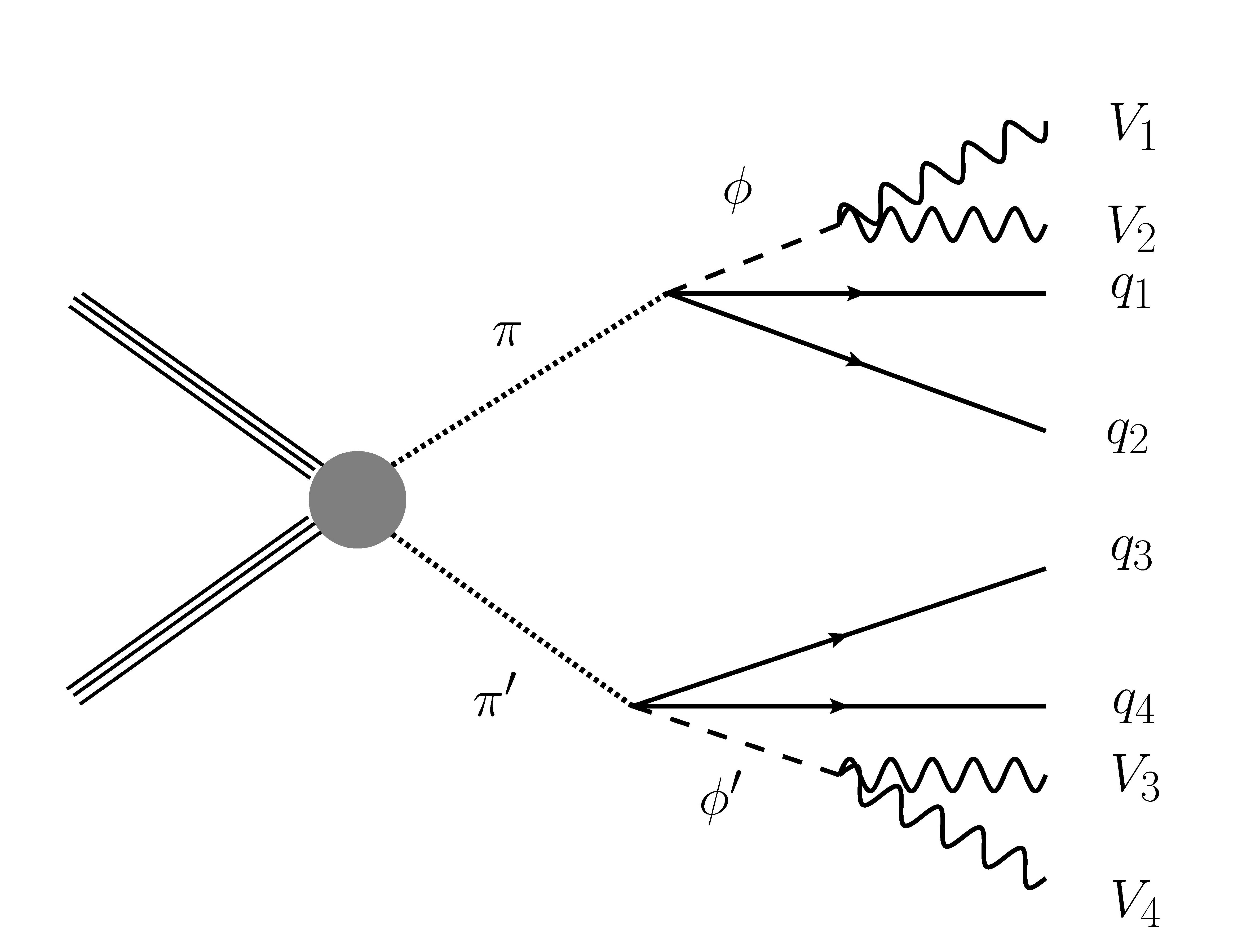
As far as fermionic colored objects go these models predict a slew of additional resonances but all of them, with the possible exception of the top partners, should be out of reach at LHC.
Exotic fermions of higher electric charge also need be taken into consideration. For the almost ubiquitous charge state , the main decay mode targeted by experiments so far is [55], but the existence of possible additional charged pNGBs opens alternative channels such as . The presence of doubly charged pNGBs in some constructions might even allow for .
The operator creating the fermionic resonance should acquire a large negative anomalous dimension in the running from to . This has been investigated at the perturbative level in [56] for the class of models in [8]. More recently [57] summarized the results for the QCD case, also within perturbation theory.
5 Two more pNGBs/ALPs
A universal feature of all of these models, simply due to the fact that they are constructed out of two different types of fermions, is the existence of two additional neutral pNGBs associated to the abelian axial currents from the axial and . One linear combination of these currents can be taken to be free of anomalies. The associated pNGB, to be denoted by , will be naturally light and, in absence of further interactions would essentially be a composite axion [58] coupling to both gluons and EW gauge bosons via the anomaly
| (39) |
Since the associated decay constant is much smaller than the possible window of values allowed by the “invisible-axion” solution, we must give this particle a mass to avoid the usual constraints. As in technicolor models [59], a mass can be obtained from e.g. the four-fermi terms arising at the scale of the type ()
| (40) |
For typical values of the parameters, using Dashen’s formula [60] we estimate
| (41) |
but a fairly large range of masses is possible. For instance, Naive Dimensional Analysis would lead to a lower estimate . This value needs to be raised at least by roughly a factor in order not to conflict with the bounds on the visible axion, coming from beam dump experiments (discussed in [61]) or searches [62]. (See also [63] for cosmological bounds for ALPS at much higher scale .) This however is easily achieved. In fact, in [23] the exciting possibility has been raised that this object is responsible for the 750 GeV bump in the di-photon signal recently reported by ATLAS and CMS [22]. Such a large mass could be obtained by e.g. adding bare masses for the colored hyperquarks.
The remaining linear combination, to be denoted by , corresponds to the anomalous current and its associated “would-be” Goldstone boson acquires a mass via the ’t Hooft mechanism [64]. The mass is given the Veneziano-Witten formula [65, 66] (, the topological susceptibility)
| (42) |
that can be naively estimated to be of the same order of a typical resonance. However, subtleties may arise that lower the mass of this object and also make it within reach of the LHC.

Regardless of their mass, these objects are singly produced mostly by gluons via the anomaly and decay to di-bosons also via the anomaly (Fig. 8) with calculable branching ratios. This makes them a good window into UV physics since the branching ratios are related to the type of UV d.o.f. of the underlying theory. It would also be interesting to investigate in detail the mixing of these scalars with the other fields in the EW coset, as done recently in [67] in the context of the model [47]. This could lead to an enhancement in the cross-section for the EW pNGBs.
Acknowledgments
The author wishes to thank A. Belyaev, G. Cacciapaglia, T. Flacke, M. Frigerio, M. Golterman, A. Hallin, D. Karateev, A. Padellaro, C. Pettersson, C. Pica, F. Sannino, Y. Shamir and L. Vecchi for discussion. The author would also like to express a special thanks to the Mainz Institute for Theoretical Physics (MITP) for its hospitality and support.
Appendix A All models of partial compositeness satisfying the requirements in the text
In this appendix we list all models of partial compositeness satisfying the requirements in the text. The main requirements are a simple hypercolor gauge group and two irreps and giving rise to a custodial EW coset and top partners. In addition, we require the theory to be asymptotically free and of course free of gauge anomalies.
Comparing with [10] we have removed a few models that do not seem promising. Some are based on spinorial irreps of the orthogonal group for which, as discussed in [10], the MAC hypothesis leads to the wrong symmetry breaking pattern. Others are those having baryons of type with in a complex irrep. This leads to top partners in the violating the custodial symmetry [36].
If the di-photon excess [22] will be confirmed with properties roughly in agreement with the 2015 data, only a fraction of models [23] will be able to fit the data. Further restrictions [68] could arise from imposing ’t Hooft anomaly matching [69].
| Restrictions | Top-partners | |||
| Real | Real | |||
| Real | Pseudo-Real | |||
| Real | Complex | |||
| Pseudo-Real | Real | |||
| Complex | Real | |||
| Complex | Complex | |||
The list of models presented in Table 5 contains both conformal and confining theories.
It is unfortunately not yet possible to exactly identify the conformal region in non-supersymmetric gauge theories. However, one can use some heuristic arguments to get indications on their behavior and it turns out that most of the models are rather clear-cut cases. Consider for instance the two-loop beta-function . ( always.) A formal solution to exists for and, if not to large, it can be trusted and the theory can be assumed to be in the conformal regime. If or is out of the perturbative regime, the model is likely to be confining. In between there is a region, difficult to characterize precisely, where the theory is conformal but strongly coupled.
In Table 6 we list the subset of models that are likely to be outside of the conformal window. These models also obey the heuristic bound proposed in [70] as well as the rigorous bounds from the -theorem [71] .
| Restrictions | ||||
|---|---|---|---|---|
The use of these models for BSM physics depends on their IR behavior. The simplest application would be to restrict oneself to the models in Table 6. These models can be easily brought into the conformal window from the strong coupling side by adding additional matter. The most straightforward way of achieving this is to have additional fermions, possibly in the same irreps, with masses at the scale . In this case one has a concrete way to put the theory in the “strongest possible” conformal point where the anomalous dimensions of the top-partners may be large enough. The theory then exits the conformal point at the scale , where the additional d.o.f. decouple. However, models outside of this class might still be amenable to other applications and we decided to keep them in the full classification of Table 5.
Appendix B Group theory conventions for the three cosets
In this appendix we collect the conventions for the explicit constructions of the three EW cosets studied in the text.
B.1 Notation for the coset
In this case we realize the Lie algebra of the unbroken group as the subset of antisymmetric imaginary generators of . This is just a particular choice of basis; a more general way of doing the decomposition is to introduce a symmetric matrix and define the broken/unbroken generators as respectively. We chose not to do this, and set from the onset but comment below on the general form of the pNGB matrix in the general case. The generators of the custodial are chosen to be
The broken generators are the real symmetric traceless generators of . We write the pNGBs as
| (75) |
| (76) |
| (77) |
| (78) |
In this way with our conventions the full matrix of pNGBs is real symmetric::
| (79) |
The vacuum misalignment is described by the following unitary matrix obtained by exponentiating (half of) the Higgs v.e.v.
| (80) |
preserves the custodial symmetry generated by and we write the non-linear realization of the pNGBs as a symmetric and unitary matrix
| (81) |
All the fields in have zero v.e.v. and in the unitary gauge and .
Notice that with our choice of basis, . Had we chosen a more general , we would have obtained
| (82) |
where the last identity defines . The matrix has the advantage of making some formulas look more uniform in all three cases but the disadvantage of not transforming uniformly under and we chose not to use it. The covariant derivative is
| (83) |
and in our convention can be written in terms of commutators. Finally, the kinetic term is
| (84) |
B.2 Notation for the coset
We pick the symplectic matrix
| (85) |
The unbroken generators satisfy . In particular, the generators of are chosen to be
and the pNGBs can be represented as
| (121) |
Notice that .
The matrix describing vacuum misalignment and preserving the custodial symmetry is
| (122) |
in terms of which the non-linear realization can be expressed as an anti-symmetric and unitary matrix
| (123) |
Also in this case, the fields in have zero v.e.v. and in the unitary gauge and . The covariant derivative reads as in the previous case (83) but the kinetic term is normalized differently
| (124) |
Even in this case one has the option of using and of introducing a matrix through the identity in an analogous way as for the previous coset, but we do not use it for the same reasons as above.
B.3 Notation for the coset
In this case, the subgroup is embedded in the unbroken by choosing
The pNGBs are parameterized as follows
where and . In the unitary gauge we have as usual , , having chosen to rotate the v.e.v. into the first of the two doublets. The neutral component of the second doublet is thus physical and can be written as a CP even plus CP odd part: . Finally we set
| (169) |
and, for the vacuum misalignment matrix we obtain
| (170) |
In this case, the non linear realization of the pNGBs is given by the unitary matrix
| (171) |
The covariant derivative is obtained by the usual commutator
| (172) |
and the kinetic term is normalized as
| (173) |
Appendix C Additional three and four bosons couplings for the models in the text.
Additional (i.e. other than those involving ) quartic couplings for are shown in (174) (in agreement with [21]).
| (174) |
The anomalous cubic couplings for are shown in Table 7. Each coupling should be multiplied by .
Finally, we present in eq. (175) the additional (i.e. other than those involving ) quartic couplings for .
Of course, the generation of masses by the potential introduces a mixing between these gauge eigenstates. This depends on the specific nature of the mass matrix and in many cases it could be handled by the mass insertion approximation. Throughout the paper we work with gauge eigenstates. Also note that one could use the Clebsch - Gordan coefficients to express the gauge eigenstates as eigenstates of the diagonal custodial symmetry group as done in [32]. An even deeper difference with the model in [32] is that they used an additional gauge field to induce vacuum-misalignment instead of top coupling.
| Fields | Couplings | Fields | Couplings | Fields | Couplings |
|---|---|---|---|---|---|
| (175) |
References
- [1] F. Englert and R. Brout, Phys. Rev. Lett. 13 (1964) 321. P. W. Higgs, Phys. Rev. Lett. 13 (1964) 508. G. S. Guralnik, C. R. Hagen and T. W. B. Kibble, Phys. Rev. Lett. 13 (1964) 585.
- [2] S. Weinberg, Phys. Rev. Lett. 19 (1967) 1264.
- [3] D. B. Kaplan and H. Georgi, Phys. Lett. B 136 (1984) 183.
- [4] D. B. Kaplan, Nucl. Phys. B 365 (1991) 259.
- [5] S. R. Coleman, J. Wess and B. Zumino, Phys. Rev. 177 (1969) 2239. C. G. Callan, Jr., S. R. Coleman, J. Wess and B. Zumino, Phys. Rev. 177 (1969) 2247.
- [6] R. Contino, arXiv:1005.4269 [hep-ph]. G. Panico and A. Wulzer, Lect. Notes Phys. 913 (2016) pp.1 [arXiv:1506.01961 [hep-ph]].
- [7] J. Barnard, T. Gherghetta and T. S. Ray, JHEP 1402 (2014) 002 [arXiv:1311.6562 [hep-ph]].
- [8] G. Ferretti, JHEP 1406 (2014) 142 [arXiv:1404.7137 [hep-ph]].
- [9] L. Vecchi, arXiv:1506.00623 [hep-ph].
- [10] G. Ferretti and D. Karateev, JHEP 1403 (2014) 077 [arXiv:1312.5330 [hep-ph] (V2)].
- [11] F. Caracciolo, A. Parolini and M. Serone, JHEP 1302 (2013) 066 [arXiv:1211.7290 [hep-ph]]. D. Marzocca, A. Parolini and M. Serone, JHEP 1403 (2014) 099 [arXiv:1312.5664 [hep-ph]].
- [12] R. Nevzorov and A. W. Thomas, Phys. Rev. D 92 (2015) 075007 [arXiv:1507.02101 [hep-ph]]. N. Bizot and M. Frigerio, JHEP 1601 (2016) 036 [arXiv:1508.01645 [hep-ph]]. V. Sanz and J. Setford, JHEP 1512 (2015) 154 [arXiv:1508.06133 [hep-ph]].
- [13] A. De Simone, O. Matsedonskyi, R. Rattazzi and A. Wulzer, JHEP 1304 (2013) 004 [arXiv:1211.5663 [hep-ph]]. A. Thamm, R. Torre and A. Wulzer, JHEP 1507 (2015) 100 [arXiv:1502.01701 [hep-ph]]. J. Barnard and M. White, JHEP 1510 (2015) 072 [arXiv:1507.02332 [hep-ph]]. D. Croon, B. M. Dillon, S. J. Huber and V. Sanz, arXiv:1510.08482 [hep-ph]. M. J. Schlaffer, DESY-THESIS-2015-036. C. Englert, R. Rosenfeld, M. Spannowsky and A. Tonero, arXiv:1603.05304 [hep-ph].
- [14] M. A. Luty and T. Okui, JHEP 0609 (2006) 070 [hep-ph/0409274].
- [15] M. J. Strassler, hep-th/0309122.
- [16] R. Rattazzi, V. S. Rychkov, E. Tonni and A. Vichi, JHEP 0812 (2008) 031 [arXiv:0807.0004 [hep-th]]. V. S. Rychkov and A. Vichi, Phys. Rev. D 80 (2009) 045006 [arXiv:0905.2211 [hep-th]].
- [17] C. Vafa and E. Witten, Nucl. Phys. B 234 (1984) 173.
- [18] O. Matsedonskyi, JHEP 1502 (2015) 154 [arXiv:1411.4638 [hep-ph]].
- [19] G. Cacciapaglia, H. Cai, T. Flacke, S. J. Lee, A. Parolini and H. Serodio, JHEP 1506 (2015) 085 [arXiv:1501.03818 [hep-ph]].
- [20] G. Panico and A. Pomarol, arXiv:1603.06609 [hep-ph].
- [21] T. Ma and G. Cacciapaglia, JHEP 1603 (2016) 211 [arXiv:1508.07014 [hep-ph]].
- [22] The ATLAS collaboration, ATLAS-CONF-2015-081. CMS Collaboration [CMS Collaboration], CMS-PAS-EXO-15-004.
- [23] A. Belyaev, G. Cacciapaglia, H. Cai, T. Flacke, A. Parolini and H. Serodio, arXiv:1512.07242 [hep-ph].
- [24] B. Bellazzini, R. Franceschini, F. Sala and J. Serra, JHEP 1604 (2016) 072 [arXiv:1512.05330 [hep-ph]].
- [25] Z. y. Duan, P. S. Rodrigues da Silva and F. Sannino, Nucl. Phys. B 592 (2001) 371 [hep-ph/0001303].
- [26] E. Katz, A. E. Nelson and D. G. E. Walker, JHEP 0508 (2005) 074 [hep-ph/0504252].
- [27] P. Lodone, JHEP 0812 (2008) 029 [arXiv:0806.1472 [hep-ph]].
- [28] B. Gripaios, A. Pomarol, F. Riva and J. Serra, JHEP 0904 (2009) 070 [arXiv:0902.1483 [hep-ph]].
- [29] G. Cacciapaglia and F. Sannino, JHEP 1404 (2014) 111 [arXiv:1402.0233 [hep-ph]].
- [30] M. Schmaltz, D. Stolarski and J. Thaler, JHEP 1009 (2010) 018 [arXiv:1006.1356 [hep-ph]].
- [31] H. Georgi and D. B. Kaplan, Phys. Lett. B 145 (1984) 216.
- [32] M. J. Dugan, H. Georgi and D. B. Kaplan, Nucl. Phys. B 254 (1985) 299.
- [33] N. Arkani-Hamed, A. G. Cohen, E. Katz and A. E. Nelson, JHEP 0207 (2002) 034 [hep-ph/0206021].
- [34] L. Vecchi, arXiv:1304.4579 [hep-ph].
- [35] J. Mrazek, A. Pomarol, R. Rattazzi, M. Redi, J. Serra and A. Wulzer, Nucl. Phys. B 853 (2011) 1 [arXiv:1105.5403 [hep-ph]].
- [36] K. Agashe, R. Contino, L. Da Rold and A. Pomarol, Phys. Lett. B 641 (2006) 62 [hep-ph/0605341].
- [37] P. Sikivie, L. Susskind, M. B. Voloshin and V. I. Zakharov, Nucl. Phys. B 173 (1980) 189.
- [38] S. R. Coleman and E. J. Weinberg, Phys. Rev. D 7 (1973) 1888.
- [39] T. DeGrand, Y. Liu, E. T. Neil, Y. Shamir and B. Svetitsky, Phys. Rev. D 91 (2015) 11, 114502 [arXiv:1501.05665 [hep-lat]]. T. DeGrand, Y. Liu, E. T. Neil, Y. Shamir and B. Svetitsky, PoS LATTICE 2014 (2014) 275 [arXiv:1412.4851 [hep-lat]].
- [40] T. DeGrand, doi:10.1103/RevModPhys.88.015001 arXiv:1510.05018 [hep-ph].
- [41] D. K. Hong, S. D. H. Hsu and F. Sannino, Phys. Lett. B 597 (2004) 89 [hep-ph/0406200]. D. D. Dietrich, F. Sannino and K. Tuominen, Phys. Rev. D 72 (2005) 055001 [hep-ph/0505059]. D. D. Dietrich and F. Sannino, Phys. Rev. D 75 (2007) 085018 [hep-ph/0611341].
- [42] M. Golterman and Y. Shamir, Phys. Rev. D 91 (2015) 9, 094506 [arXiv:1502.00390 [hep-ph]].
- [43] K. Agashe, R. Contino and A. Pomarol, Nucl. Phys. B 719 (2005) 165 [hep-ph/0412089].
- [44] G. Aad et al. [ATLAS Collaboration], Phys. Lett. B 716 (2012) 1 [arXiv:1207.7214 [hep-ex]]. S. Chatrchyan et al. [CMS Collaboration], Phys. Lett. B 716 (2012) 30 [arXiv:1207.7235 [hep-ex]].
- [45] J. Wess and B. Zumino, Phys. Lett. B 37 (1971) 95. E. Witten, Nucl. Phys. B 223, 422 (1983).
- [46] O. Kaymakcalan, S. Rajeev and J. Schechter, Phys. Rev. D 30 (1984) 594.
- [47] H. Georgi and M. Machacek, Nucl. Phys. B 262 (1985) 463.
- [48] J. Alwall et al., JHEP 1407 (2014) 079 [arXiv:1405.0301 [hep-ph]]. A. Alloul, N. D. Christensen, C. Degrande, C. Duhr and B. Fuks, Comput. Phys. Commun. 185 (2014) 2250 [arXiv:1310.1921 [hep-ph]].
- [49] M. Frigerio, A. Pomarol, F. Riva and A. Urbano, JHEP 1207 (2012) 015 [arXiv:1204.2808 [hep-ph]].
- [50] M. Kim, S. J. Lee and A. Parolini, arXiv:1602.05590 [hep-ph].
- [51] A. Joseph and S. G. Rajeev, Phys. Rev. D 80 (2009) 074009 [arXiv:0905.2772 [hep-ph]].
- [52] L. Calibbi, G. Ferretti, D. Milstead, C. Petersson and R. Pöttgen, arXiv:1602.04821 [hep-ph].
- [53] B. Gripaios, JHEP 1002 (2010) 045 [arXiv:0910.1789 [hep-ph]].
- [54] G. Cacciapaglia, H. Cai, A. Deandrea, T. Flacke, S. J. Lee and A. Parolini, JHEP 1511 (2015) 201 [arXiv:1507.02283 [hep-ph]].
- [55] S. Chatrchyan et al. [CMS Collaboration], Phys. Rev. Lett. 112 (2014) no.17, 171801 [arXiv:1312.2391 [hep-ex]].
- [56] T. DeGrand and Y. Shamir, Phys. Rev. D 92 (2015) no.7, 075039 [arXiv:1508.02581 [hep-ph]].
- [57] C. Pica and F. Sannino, arXiv:1604.02572 [hep-ph].
- [58] J. E. Kim, Phys. Rev. D 31 (1985) 1733.
- [59] E. Farhi and L. Susskind, Phys. Rept. 74 (1981) 277.
- [60] R. F. Dashen, Phys. Rev. 183 (1969) 1245.
- [61] B. Dobrich, J. Jaeckel, F. Kahlhoefer, A. Ringwald and K. Schmidt-Hoberg, JHEP 1602 (2016) 018 [arXiv:1512.03069 [hep-ph]].
- [62] V. V. Anisimovsky et al. [E949 Collaboration], Phys. Rev. Lett. 93 (2004) 031801 [hep-ex/0403036].
- [63] D. Cadamuro and J. Redondo, JCAP 1202 (2012) 032 [arXiv:1110.2895 [hep-ph]].
- [64] G. ’t Hooft, Phys. Rev. Lett. 37 (1976) 8.
- [65] G. Veneziano, Nucl. Phys. B 159 (1979) 213.
- [66] E. Witten, Nucl. Phys. B 156 (1979) 269.
- [67] K. Howe, S. Knapen and D. J. Robinson, arXiv:1603.08932 [hep-ph].
- [68] G. Cacciapaglia and A. Parolini, Phys. Rev. D 93 (2016) no.7, 071701 [arXiv:1511.05163 [hep-ph]].
- [69] G. ’t Hooft, NATO Adv. Study Inst. Ser. B Phys. 59 (1980) pp.1.
- [70] F. Sannino, Phys. Rev. D 79 (2009) 096007 [arXiv:0902.3494 [hep-ph]]. T. A. Ryttov and F. Sannino, Int. J. Mod. Phys. A 25 (2010) 4603 [arXiv:0906.0307 [hep-ph]].
- [71] J. L. Cardy, Phys. Lett. B 215 (1988) 749. H. Osborn, Phys. Lett. B 222 (1989) 97. I. Jack and H. Osborn, Nucl. Phys. B 343 (1990) 647.