跳到论文正文
W Papers独立论文阅读器 arXiv:1604.06452 论文正文 计算阅读时间 · 0%
引用这篇论文根据当前论文元数据生成,正式投稿前建议核对。


License: arXiv.org perpetual non-exclusive license
arXiv:1604.06452v1 [cs.DS] 21 Apr 2016

Weighted domination number of cactus graphs

Tina Novak

University of Ljubljana, Faculty of Mechanical Engineering

Aškerčeva 6, SI-1000 Ljubljana, Slovenia

tina.novak@fs.uni-lj.si

Janez Žerovnik

University of Ljubljana, Faculty of Mechanical Engineering

Aškerčeva 6, SI-1000 Ljubljana, Slovenia

janez.zerovnik@fs.uni-lj.si

Abstract: In the paper, we write a linear algorithm for calculating the weighted domination number of a vertex-weighted cactus. The algorithm is based on the well known depth first search (DFS) structure. Our algorithm needs less than 12​n+5​b12n+5b additions and 9​n+2​b9n+2b min\min-operations where nn is the number of vertices and bb is the number of blocks in the cactus.

Keywords: weighted domination problem,cactus graph, DFS structure

1 Introduction

Cactus graphs are interesting generalizations of trees, with numerous applications, for example in location theory [3, 17], communication networks [8, 18], stability analysis [1], and elsewhere. Usually, linear problems on trees imply linear problems on cacti. In this paper, we study the weighted domination number of a cactus graph with weighted vertices. It is well known that the problem of the weighted domination number on trees is linear [5, 12]. Actually, we also have very general linear algorithm for computing domination-like problems on partial kk-trees [13]. Time complexity of this algorithm is 𝒪⁡(n​|L|2​k+1){\cal O}(n|L|^{2k+1}), where kk is the treewidth and LL is the set of vertex states (the different ways that a solution to a subproblem impact to the origin vertex). In the case of cactus graphs we have k=2k=2 and |L|=3|L|=3. Therefore, the time complexity of the general algorithm [13] on cacti is 𝒪⁡(35​n){\cal O}(3^{5}n).

It is well known that cactus graphs can be recognized by running an extended version of depth first search (DFS) algorithm that results a data structure of a cactus, see for example [16]. From the data structure, the vertices can be naturally divided into three types, i.e. each vertex either lies on a cycle and has degree 22 or lies on a cycle and has degree ≥3\geq 3 or does not lie on a cycle (see [4]). Using this structure, we design an algorithm for general cacti. In the paper, we first illustrate the basic idea by writing a version of the algorithm for trees before generalizing the approach to arbitrary cactus graphs. Our algorithm has time complexity 𝒪⁡(28​n){\cal O}(28n) which substantially improves the constant 35=2433^{5}=243. In fact, we will estimate time complexity of our algorithm more precisely (blocks will be formally defined later)

Theorem 1

Let nn be the number of vertices in a cactus and b<nb<n be the number of blocks. For computing the weighted domination number we need less than 12​n+5​b12n+5b additions and 9​n+2​b9n+2b min\min-operations.

The rest of the paper is organized as follows. In the next section we first recall definitions of the domination number and the weighted domination number of general graphs. For cacti, we introduce the classification of vertices in relation to the skeleton structure [4]. In Section 3 we define three parameters that are useful when considering the weighted domination problem. The simplified version of the algorithm that is used for computing the weighted domination number of a tree is presented in Section 4. Special cases of graphs, i.e. path-like graphs and cycle-like graphs are regarded in Section 5. We write algorithms for calculating their weighted domination parameters and weighted domination number. In Section 6, the algorithm for general cacti is given and its time complexity is estimated.

2 Definitions and preliminaries

A vertex-weighted graph and the weighted domination number

Let G=(V,E)G=(V,E) be a graph with a set of vertices V=V⁡(G)V=V(G) and a set of edges E=E⁡(G)E=E(G). Denote by N⁡(v)N(v) the open neighborhood of a vertex vv i.e. the set of vertices adjacent to the vertex vv and by N⁡[v]N[v] the closed neighborhood of a vertex vv: N⁡[v]={v}∪N⁡(v)N[v]=\{v\}\cup N(v). Let SS be any subset of the set of vertices VV. Denote by N⁡(S)N(S) the open neighborhood of the set SS i.e. the set of vertices adjacent to any vertex in SS and similarly by N⁡[S]N[S] the closed neighborhood of SS: N⁡[S]=S∪N⁡(S)N[S]=S\cup N(S). A subset D⊆VD\subseteq V is a dominating set if N⁡[D]=VN[D]=V. A domination number γ⁡(G)\gamma(G) is the minimum cardinality among all dominating sets of the graph GG.

In this article, a weighted graph (G,w)(G,w) is a graph together with a positive real weight-function w:V→ℝ+w:V\to{\mathbb{R}}_{+}. For the vertex vj∈Vv_{j}\in V we shall write wj=w⁡(vj)w_{j}=w(v_{j}). The weight of a dominating set DD is defined as w⁡(D)=∑vj∈Dwjw(D)=\sum_{v_{j}\in D}w_{j}. Finally, the weighted domination number (WDN) γw​(G)\gamma_{w}(G) of the graph GG is the minimum weight of a dominating set, more precisely

γw​(G)=min⁡{w⁡(D)|D​is a dominating set}.\gamma_{w}(G)=\min\Big\{w(D)\,\big|\;D\;\hbox{is a dominating set}\Big\}\;. (1)

Cactus graph and its skeleton

A graph K=(V⁡(K),E⁡(K))K=(V(K),E(K)) is a cactus graph if and only if any two cycles of KK have at most one vertex in common. Equivalently, any edge of a cactus lies on at most one cycle. Skeleton structure of a cactus is elaborated in [4], where it is shown that the vertices of a cactus graph are of three types:

  1. ∙\bullet

    CC-vertex is a vertex on a cycle of degree 2,

  2. ∙\bullet

    GG-vertex is a vertex not included in any cycle,

  3. ∙\bullet

    HH-vertex or a hinge is a vertex which is included in at least one cycle and is of degree ≥3\geq 3.

By a subtree in a cactus we mean a tree induced by a subset of GG-vertices and HH-vertices only. A graft is a maximal subtree in a cactus. A subgraph of a cactus is called a block when it is either a cycle or a graft.

Depth First Search (DFS) algorithm

The DFS is a well known method for exploring graphs. It can be used for recognizing cactus graphs providing the data structure (see [14], [16], [15], [17]). Consider, we have a cactus graph KK. We can distinguish one vertex as a root of KK and denote it by rr. After running the DFS algorithm, the vertices of KK are DFS ordered. The order is given by the order in which DFS visits the vertices. (Note that the DFS order of a graph is not unique as we can use any vertex as the starting vertex (the root) and can visit the neighbors of a vertex in any order. However, here we can assume that the DFS order is given and is fixed.)

We denote by DFN⁡(v)\mathrm{DFN}(v) the position of vv in the DFS order and we set DFN⁡(r)=0\mathrm{DFN}(r)=0. DFN\mathrm{DFN} is called the depth first number. Following [16] and [15], it is useful to store the information recorded during the DFS run in four arrays, called the DFS (cactus) data structure:

  1. ∙\bullet

    FATHER⁡(v)\mathrm{FATHER}(v) is the unique predecessor (father) of vertex vv in the rooted tree, constructed with the DFS.

  2. ∙\bullet

    ROOT⁡(v)\mathrm{ROOT}(v) is the root vertex of the cycle containing vv i.e. the first vertex of the cycle (containing vv) in the DFS order. If vv does not lie on a cycle, then ROOT⁡(v)=v\mathrm{ROOT}(v)=v. We set ROOT⁡(r)=r\mathrm{ROOT}(r)=r. (In any DFS order, if DFN⁡(w)<DFN⁡(v)\mathrm{DFN}(w)<\mathrm{DFN}(v) and ww is the root of the cycle containing vv and vv is the root of another cycle (it is a hinge), then ROOT⁡(v)=w\mathrm{ROOT}(v)=w.)

  3. ∙\bullet

    For vertices on a cycle (i.e. ROOT⁡(v)≠v\mathrm{ROOT}(v)\not=v), orientation of the cycle is given by ORIEN⁡(v)=z\mathrm{ORIEN}(v)=z, where zz is the son of ROOT⁡(v)\mathrm{ROOT}(v) that is visited on the cycle first. If ROOT⁡(v)=v\mathrm{ROOT}(v)=v , then ORIEN⁡(v)=v\mathrm{ORIEN}(v)=v.

  4. ∙\bullet

    IND⁡(v):=|{u|FATHER⁡(u)=v}|\mathrm{IND}(v):=|\{u\,\big|\;\mathrm{FATHER}(u)=v\}| is the number of sons of vv in the DFS tree.

Below we write the pseudocode of the DFS algorithm that provides the data structure of cacti. The idea is taken from [14]. To mark a visited vertex in the procedure, we introduce auxiliary array MARK\mathrm{MARK} (as in [14]). At the beginning of the algorithm, we set MARK(v)=0(v)=0 for every vertex in KK. During the algorithm, whenever a vertex vv is visited for the first time, the value MARK(v)(v) becomes 11 and DFN(v)(v) is increased by 11.

Algorithm 1 DFS algorithm
Data: Rooted cactus (K,r)(K,r) with vertices V⁡(K)V(K) and edges E⁡(K)E(K);
initialize
 i=0i=0;
 For every vertex vv in KK set
  FATHER⁡(v)=v\mathrm{FATHER}(v)=v;  MARK⁡(v)=0\mathrm{MARK}(v)=0;  ROOT⁡(v)=v\mathrm{ROOT}(v)=v;
  ORIEN⁡(v)=v\mathrm{ORIEN}(v)=v;  IND⁡(v)=0\mathrm{IND}(v)=0;  DFN⁡(v)=0\mathrm{DFN}(v)=0;
 and for the root rr reset:
  MARK⁡(r)=1\mathrm{MARK}(r)=1;
 v=rv=r;
repeat
if all the edges incident tovhave already been labeled ”examined”\hbox{\rm all the edges incident to}\;v\;\hbox{\rm have already been labeled "examined"}
  (vv is completely scaned) then
  v=FATHER⁡(v)v=\mathrm{FATHER}(v)
else (an edge (v,w)(v,w) is not labeled ”examined”)
  The edge (v,w)(v,w) label ”examined” and do the following
  if MARK⁡(w)=0\mathrm{MARK}(w)=0 then
   i=i+1i=i+1;
   DFN⁡(w)=i\mathrm{DFN}(w)=i;
   MARK⁡(w)=1\mathrm{MARK}(w)=1;
   FATHER⁡(w)=v\mathrm{FATHER}(w)=v;
   IND⁡(w)=IND⁡(v)+1\mathrm{IND}(w)=\mathrm{IND}(v)+1;
   v=wv=w.
  else(MARK⁡(w)=1\mathrm{MARK}(w)=1, that means we have a cycle)
   label the edge (w,v)(w,v) ”examined”;
   ROOT⁡(v)=w\mathrm{ROOT}(v)=w;
   u=FATHER⁡(v)u=\mathrm{FATHER}(v);
   repeat (assigning the root ww of vertices of the cycle)
     z=uz=u;
     ROOT⁡(z)=w\mathrm{ROOT}(z)=w;
     u=FATHER⁡(z)u=\mathrm{FATHER}(z);
   until u=wu=w. (now zz determines the orientation of the cycle with the
           root ww)
   repeat (assigning the successor zz i.e. the orientation of vertices of
        the cycle)
     ORIEN⁡(v)=z\mathrm{ORIEN}(v)=z;
     v=FATHER⁡(v)v=\mathrm{FATHER}(v);
   until v=wv=w.
   v=wv=w;
  end if
end if

until v=rv=r and all edges incident to rr are ”examined”
Result: arrays FATHER\mathrm{FATHER}, ROOT\mathrm{ROOT}, ORIEN\mathrm{ORIEN}, IND\mathrm{IND}, MARK\mathrm{MARK}, DFN\mathrm{DFN}.

Algorithm 2 DFS algorithm - Part 2

Direct correspondence of the definitions of CC, GG, HH-vertices in a rooted cactus (K,r)(K,r) and arrays FATHER\mathrm{FATHER}, ROOT\mathrm{ROOT}, ORIEN\mathrm{ORIEN} and IND\mathrm{IND} is described in the following lemma

Lemma 2 ((CC,GG,HH-vertices in DFS array))

  1. 1.

    For a vertex v≠rv\neq r the following holds

    1. (a)

      vv is a CC-vertex if and only if ROOT⁡(v)≠v\mathrm{ROOT}(v)\neq v and IND⁡(v)=1\mathrm{IND}(v)=1

    2. (b)

      vv is a GG-vertex if and only if ROOT⁡(v)=v\mathrm{ROOT}(v)=v and ORIEN⁡(v)=v\mathrm{ORIEN}(v)=v and for every son uu of vv we have ROOT⁡(u)≠v\mathrm{ROOT}(u)\neq v

    3. (c)

      vv is a HH-vertex if and only if either (ROOT⁡(v)=v\mathrm{ROOT}(v)=v and ORIEN⁡(v)=v\mathrm{ORIEN}(v)=v and for at least one son uu of vv we have ROOT⁡(u)=v\mathrm{ROOT}(u)=v ) or (ROOT⁡(v)≠v\mathrm{ROOT}(v)\neq v and IND⁡(v)>1\mathrm{IND}(v)>1).

  2. 2.

    For the root rr we have

    1. (a)

      rr is a CC-vertex if and only if IND⁡(r)=1\mathrm{IND}(r)=1 and for the son uu of rr (DFN⁡(u)=1\mathrm{DFN}(u)=1) we have ROOT⁡(u)=v\mathrm{ROOT}(u)=v

    2. (b)

      rr is a GG-vertex if and only if for every son uu of rr we have ROOT⁡(u)=u\mathrm{ROOT}(u)=u

    3. (c)

      rr is a HH-vertex if and only if IND⁡(r)>1\mathrm{IND}(r)>1 and for at least one son uu of rr we have ROOT⁡(u)=r\mathrm{ROOT}(u)=r.

Remark 3

For any vertex v∈V⁡(K)v\in V(K) and his father w=FATHER⁡(v)w=\mathrm{FATHER}(v), vertices with DFN\mathrm{DFN}’s

DFN⁡(w),DFN⁡(w)+1,…,DFN⁡(v)−1\mathrm{DFN}(w),\mathrm{DFN}(w)+1,\ldots,\mathrm{DFN}(v)-1

(and all corresponding edges induced by V⁡(K)V(K)) form a rooted subcactus with the root ww, denote it (K~w,w)(\widetilde{K}_{w},w). Graphs K~w\widetilde{K}_{w} and {v}\{v\} are disjoint.

Observation. Assume the last vertex ll in the DFS order of a cactus KK lies on a subtree TT in KK. Let w=FATHER⁡(l)w=\mathrm{FATHER}(l) and ww be the root (according to DFS order) of any subcactus K~w\widetilde{K}_{w}, such that {l}∩V⁡(K~w)=∅\{l\}\cap V(\widetilde{K}_{w})=\emptyset. If v~∈V⁡(K~w)\widetilde{v}\in V(\widetilde{K}_{w}), then DFN⁡(w)≤DFN⁡(v~)<DFN⁡(l)\mathrm{DFN}(w)\leq\mathrm{DFN}(\widetilde{v})<\mathrm{DFN}(l). Similar but perhaps a little less obvious fact is given in the next proposition.

Proposition 4

Consider the last vertex ll in DFS order of a cactus KK lies on a cycle CC. Then the following is true

  1. 1.

    the neighboring vertex of ll in the cycle CC, which is not the father of the vertex ll, it is the root of the cycle CC.

  2. 2.

    vertex ll is not a hinge.

  3. 3.

    let w,v∈Cw,v\in C, w=FATHER⁡(v)w=\mathrm{FATHER}(v), ww is not the root of the cycle CC and ww is a hinge, i.e. the root of a subcactus K~\widetilde{K}, such that V⁡(C)∩V⁡(K~)=wV(C)\cap V(\widetilde{K})=w. For any v~∈V⁡(K~)\widetilde{v}\in V(\widetilde{K}), we have DFN⁡(w)≤DFN⁡(v~)<DFN⁡(v)\mathrm{DFN}(w)\leq\mathrm{DFN}(\widetilde{v})<\mathrm{DFN}(v).

Proof: 

  1. 1.

    Denote by vv a neighboring vertex of ll in the cycle CC, which is not the father of ll. If vv is not the root of CC, then DFN⁡(v)>DFN⁡(l)\mathrm{DFN}(v)>\mathrm{DFN}(l). Contradiction.

  2. 2.

    If ll is a hinge, according to DFS order, there exist at least one vertex with DFN>DFN⁡(l)\mathrm{DFN}>\mathrm{DFN}(l). Contradiction.

  3. 3.

    According to DFS order, the inequality DFN⁡(w)≤DFN⁡(v~)\mathrm{DFN}(w)\leq\mathrm{DFN}(\widetilde{v}) holds. Consider there is v~∈K~\widetilde{v}\in\widetilde{K} with DFN⁡(v~)>DFN⁡(v)\mathrm{DFN}(\widetilde{v})>\mathrm{DFN}(v). Following DFS algorithm, we have then DFN⁡(v~)>DFN⁡(l)\mathrm{DFN}(\widetilde{v})>\mathrm{DFN}(l). Contradiction.

3 Weighted domination parameters (WDP)

Let GG be a graph and vv any vertex in V⁡(G)V(G). Consider the following three parameters yielding related weighted domination parameters (see [5]):

Definition 5

  1. 1.

    γw00​(G,v)=min⁡{w⁡(D)|D​is a dominating set of​G−v}=γw​(G−v)\gamma_{w}^{00}(G,v)=\min\big\{w(D)\,\big|\;D\;\hbox{is a dominating set of}\;\,G-v\big\}=\gamma_{w}(G-v)

  2. 2.

    γw1​(G,v)=min⁡{w⁡(D)|D​is a dominating set of​G​and​v∈D}\gamma_{w}^{1}(G,v)=\min\big\{w(D)\,\big|\;D\;\hbox{is a dominating set of}\;\,G\;\hbox{and}\;v\in D\big\}

  3. 3.

    γw0​(G,v)=min⁡{w⁡(D)|D​is a dominating set of​G​and​v∉D}\gamma_{w}^{0}(G,v)=\min\big\{w(D)\,\big|\;D\;\hbox{is a dominating set of}\;\,G\;\hbox{and}\;v\notin D\big\}.

It is obvious that

γw​(G)=min⁡{γw1​(G,v),γw0​(G,v)}.\gamma_{w}(G)=\min\big\{\gamma_{w}^{1}(G,v),\gamma_{w}^{0}(G,v)\big\}\,. (2)

Since a dominating set of GG, which does not contain the vertex vv is also a dominating set of G−vG-v, we have the relation

γw00​(G,v)≤γw0​(G,v).\gamma_{w}^{00}(G,v)\leq\gamma_{w}^{0}(G,v)\,. (3)

Let DD be a dominating set of G−vG-v such that w⁡(D)=γw​(G−v)w(D)=\gamma_{w}(G-v). Then D∪{v}D\cup\{v\} is a dominating set of GG and clearly

γw1​(G,v)≤w⁡(v)+γw00​(G,v).\gamma_{w}^{1}(G,v)\leq w(v)+\gamma_{w}^{00}(G,v)\,. (4)
Lemma 6

Let G1G_{1} and G2G_{2} be disjoined rooted graphs with roots v1v_{1} and v2v_{2} respectively, and let GG be a disjoint union of G1G_{1} and G2G_{2} joined by the edge v1​v2v_{1}v_{2}. Then the following is true:

  1. 1.

    γw00​(G,v1)=γw00​(G1,v1)+γw​(G2)\gamma_{w}^{00}(G,v_{1})=\gamma_{w}^{00}(G_{1},v_{1})+\gamma_{w}(G_{2}),

  2. 2.

    γw1​(G,v1)=γw1​(G1,v1)+min⁡{γw1​(G2,v2),γw00​(G2,v2)}\gamma_{w}^{1}(G,v_{1})=\gamma_{w}^{1}(G_{1},v_{1})+\min\big\{\gamma_{w}^{1}(G_{2},v_{2}),\gamma_{w}^{00}(G_{2},v_{2})\big\},

  3. 3.

    γw0​(G,v1)=min⁡{γw0​(G1,v1)+γw​(G2,v2),γw00​(G1,v1)+γw1​(G2,v2)}\gamma_{w}^{0}(G,v_{1})=\min\big\{\gamma_{w}^{0}(G_{1},v_{1})+\gamma_{w}(G_{2},v_{2}),\gamma_{w}^{00}(G_{1},v_{1})+\gamma_{w}^{1}(G_{2},v_{2})\big\}.

The proof of Lemma 6 (for the domination number) appears in [5]. Generalization to weighted domination is straightforward and therefore ommited. A more general situation is described by the next lemma

Lemma 7

Let G1G_{1} and G2G_{2} be graphs with one common vertex v0v_{0} and let G1−v0G_{1}-v_{0} and G2−v0G_{2}-v_{0} be disjoined. Denote by GG the union of G1G_{1} and G2G_{2}. Then we have

  1. 1.

    γw00​(G,v0)=γw00​(G1,v0)+γw00​(G2,v0)\gamma_{w}^{00}(G,v_{0})=\gamma_{w}^{00}(G_{1},v_{0})+\gamma_{w}^{00}(G_{2},v_{0}),

  2. 2.

    γw1​(G,v0)=γw1​(G1,v0)+γw1​(G2,v0)−w⁡(v0)\gamma_{w}^{1}(G,v_{0})=\gamma_{w}^{1}(G_{1},v_{0})+\gamma_{w}^{1}(G_{2},v_{0})-w(v_{0}),

  3. 3.

    γw0​(G,v0)=min⁡{γw0​(G1,v0)+γw00​(G2,v0),γw00​(G1,v0)+γw0​(G2,v0)}\gamma_{w}^{0}(G,v_{0})=\min\big\{\gamma_{w}^{0}(G_{1},v_{0})+\gamma_{w}^{00}(G_{2},v_{0}),\gamma_{w}^{00}(G_{1},v_{0})+\gamma_{w}^{0}(G_{2},v_{0})\big\} .

Proof: 

  1. 1.

    As G1−v0G_{1}-v_{0} and G2−v0G_{2}-v_{0} are disjoined, it follows γw00​(G,v0)=γw00​(G1,v0)+γw00​(G2,v0).\gamma_{w}^{00}(G,v_{0})=\gamma_{w}^{00}(G_{1},v_{0})+\gamma_{w}^{00}(G_{2},v_{0}).

  2. 2.

    Let DD be a dominating set of GG with v0∈Dv_{0}\in D such that w⁡(D)=γw1​(G,v0)w(D)=\gamma_{w}^{1}(G,v_{0}). Then D1=D∩V⁡(G1)D_{1}=D\cap V(G_{1}) is a dominating set of G1G_{1} and w⁡(D1)≥γw1​(G1,v0)w(D_{1})\geq\ \gamma_{w}^{1}(G_{1},v_{0}). Similarly, D2=D∩V⁡(G2)D_{2}=D\cap V(G_{2}) is a dominating set of G2G_{2} and w⁡(D2)≥γw1​(G2,v0)w(D_{2})\geq\gamma_{w}^{1}(G_{2},v_{0}). Hence γw1​(G,v0)≥γw1​(G1,v0)+γw1​(G2,v0)−w⁡(v0)\gamma_{w}^{1}(G,v_{0})\geq\gamma_{w}^{1}(G_{1},v_{0})+\gamma_{w}^{1}(G_{2},v_{0})-w(v_{0}). On the other hand, for any dominating sets D1D_{1} and D2D_{2} with w⁡(D1)≥γw1​(G1,v0)w(D_{1})\geq\ \gamma_{w}^{1}(G_{1},v_{0}) and w⁡(D2)≥γw1​(G2,v0)w(D_{2})\geq\gamma_{w}^{1}(G_{2},v_{0}), D=D1∪D2D=D_{1}\cup D_{2} dominates GG. As D1∩D2={v0}D_{1}\cap D_{2}=\{v_{0}\}, we have w⁡(D)=w⁡(D1)+w⁡(D2)−w⁡(v0)w(D)=w(D_{1})+w(D_{2})-w(v_{0}) and therefore γw1​(G,v0)≤w⁡(D)=γw1​(G1,v0)+γw1​(G2,v0)−w⁡(v0)\gamma_{w}^{1}(G,v_{0})\leq w(D)=\gamma_{w}^{1}(G_{1},v_{0})+\gamma_{w}^{1}(G_{2},v_{0})-w(v_{0}).

  3. 3.

    As we consider only dominating sets with v0∉Dv_{0}\not\in D, v0v_{0} has to be dominated by some other vertex. We distinguish three cases: either v0v_{0} is dominated by D1=D∩V⁡(G1)D_{1}=D\cap V(G_{1}) , or D2=D∩V⁡(G2)D_{2}=D\cap V(G_{2}), or by both D1D_{1} and D2D_{2}. Assuming w⁡(D)=γw0​(G,v0)w(D)=\gamma_{w}^{0}(G,v_{0}), and recalling that γw00​(Gi,v0)≤γw0​(Gi,v0CLOSE\gamma_{w}^{00}(G_{i},v_{0})\leq\gamma_{w}^{0}(G_{i},v_{0} for i=1,2i=1,2, it follows

    γw0​(G,v0)\displaystyle\gamma_{w}^{0}(G,v_{0}) =\displaystyle\!\!= min{γw0(G1,v0)+γw00(G2,v0),γw00(G1,v0)+γw0(G2,v0),\displaystyle\!\!\min\big\{\gamma_{w}^{0}(G_{1},v_{0})+\gamma_{w}^{00}(G_{2},v_{0}),\gamma_{w}^{00}(G_{1},v_{0})+\gamma_{w}^{0}(G_{2},v_{0}),
    γw0(G1,v0)+γw0(G2,v0)}≥\displaystyle\!\!\qquad\;\,\gamma_{w}^{0}(G_{1},v_{0})+\gamma_{w}^{0}(G_{2},v_{0})\big\}\geq
    ≥\displaystyle\!\!\geq min⁡{γw0​(G1,v0)+γw00​(G2,v0),γw00​(G1,v0)+γw0​(G2,v0)}.\displaystyle\!\!\min\big\{\gamma_{w}^{0}(G_{1},v_{0})+\gamma_{w}^{00}(G_{2},v_{0}),\gamma_{w}^{00}(G_{1},v_{0})+\gamma_{w}^{0}(G_{2},v_{0})\big\}\,.

    On the other hand, we can construct dominating sets of GG by taking a union of two dominating sets D1D_{1} and D2D_{2} of G1G_{1} and G2G_{2} respectively. At least one of D1D_{1}, D2D_{2} (or both) must dominate v0v_{0}. Taking either (w⁡(D1)=γw0​(G1,v0)w(D_{1})=\gamma_{w}^{0}(G_{1},v_{0}) and w⁡(D2)=γw00​(G2,v0)w(D_{2})=\gamma_{w}^{00}(G_{2},v_{0})) or (w⁡(D1)=γw00​(G1,v0)w(D_{1})=\gamma_{w}^{00}(G_{1},v_{0}) and w⁡(D2)=γw0​(G2,v0)w(D_{2})=\gamma_{w}^{0}(G_{2},v_{0})), we conclude

    min{γw0(G1,v0)+γw00(G2,v0),γw00(G1,v0)+γw0(G2,v0),\displaystyle\min\big\{\gamma_{w}^{0}(G_{1},v_{0})+\gamma_{w}^{00}(G_{2},v_{0}),\gamma_{w}^{00}(G_{1},v_{0})+\gamma_{w}^{0}(G_{2},v_{0}),
    γw0(G1,v0)+γw0(G2,v0)}\displaystyle\gamma_{w}^{0}(G_{1},v_{0})+\gamma_{w}^{0}(G_{2},v_{0})\big\} ≥\displaystyle\!\!\geq
    ≥min⁡{γw0​(G1,v0)+γw00​(G2,v0),γw00​(G1,v0)+γw0​(G2,v0)}\displaystyle\geq\min\big\{\gamma_{w}^{0}(G_{1},v_{0})+\gamma_{w}^{00}(G_{2},v_{0}),\gamma_{w}^{00}(G_{1},v_{0})+\gamma_{w}^{0}(G_{2},v_{0})\big\} ≥\displaystyle\!\!\geq γw0​(G,v0).\displaystyle\!\!\gamma_{w}^{0}(G,v_{0}).

4 Algorithm for trees

In this section, let G=(V,E)G=(V,E) be a vertex-weighted tree, and let TT be an associated rooted tree with root rr (rr can be arbitrary but fixed vertex in V⁡(G)V(G) ). In [12], the authors write the algorithm for calculating the weighted domination of a vertex-edge-weighted tree. It can of course be applied to a vertex-weighted tree, the case of interest in this paper. Another algorithm for calculating the weighted domination number of a tree appears in [5]. We write a new algorithm for weighted domination number of a weighted tree based on the DFS data structure here in order to illustrate the main idea on a well understood special case in order to clarify the development of the general algorithm in the following sections.
Refer to caption
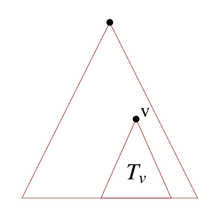
Figure 1: The rooted subtree

Denote by (Tv,v)(T_{v},v) the rooted subtree with the root vv as is shown in Figure 1. In our algorithm we use the DFS order of vertices (i.e. the DFS cactus data structure provided by the DFS algorithm). We supplement the DFS data structure by four arrays of the initial values of the parameters γw00\gamma_{w}^{00}, γw1\gamma_{w}^{1}, γw0\gamma_{w}^{0} and γw\gamma_{w}. Initially, we set for every vertex vv

γw00(v)=0,γw1=w(v),γw0=∞andγw(v)=w(v).\gamma_{w}^{00}(v)=0,\quad\gamma_{w}^{1}=w(v),\quad\gamma_{w}^{0}=\infty\quad\hbox{and}\quad\gamma_{w}(v)=w(v)\,. (5)

The algorithm’s starting point is the last vertex vv in the DFS order with the corresponding parameters γw00​(v)\gamma_{w}^{00}(v), γw1​(v)\gamma_{w}^{1}(v), γw0​(v)\gamma_{w}^{0}(v) and γw​(v)\gamma_{w}(v). In the data structure we find the father of vv and call it ww. If DFN⁡(w)≠DFN⁡(v)−1\mathrm{DFN}(w)\neq\mathrm{DFN}(v)-1 (i.e. DFN⁡(w)<DFN⁡(v)−1\mathrm{DFN}(w)<\mathrm{DFN}(v)-1), there exists rooted subtree (T~w,w)(\widetilde{T}_{w},w) (see Remark 3). The algorithm calls itself recursively for the subtree T~w\widetilde{T}_{w} and then accordingly updates the parameters γw00​(w)=γw00​(T~w,w)\gamma_{w}^{00}(w)=\gamma_{w}^{00}(\widetilde{T}_{w},w), γw1​(w)=γw1​(T~w,w)\gamma_{w}^{1}(w)=\gamma_{w}^{1}(\widetilde{T}_{w},w), γw0​(w)=γw0​(T~w,w)\gamma_{w}^{0}(w)=\gamma_{w}^{0}(\widetilde{T}_{w},w) and γw​(w)=γw​(T~w)\gamma_{w}(w)=\gamma_{w}(\widetilde{T}_{w}). When ww and vv are the last two vertices in the DFS order, the parameters at ww are computed according to Lemma 6, and the computation continues regarding ww as the last vertex. For pseudocode of the algorithm see Algorithm 3.

Refer to caption
Figure 2: Subtrees TvT_{v}, T~w\widetilde{T}_{w} and TwT_{w}
Algorithm 3 TREE
Data: A rooted tree (T,r)(T,r) with DFS ordered vertices in the DFS table
initialize γw00​(v)=0\gamma_{w}^{00}(v)=0, γw1​(v)=w⁡(v)\gamma_{w}^{1}(v)=w(v), γw0​(v)=∞\gamma_{w}^{0}(v)=\infty and γw​(v)=w​(v)\gamma_{w}(v)=w(v) for every vertex vv in the DFS table
set vv is the last vertex in the DFS order;
repeat
w=FATHER⁡(v)w=\mathrm{FATHER}(v);
if DFN⁡(w)≠DFN⁡(v)−1\mathrm{DFN}(w)\neq\mathrm{DFN}(v)-1 then
  call algorithm TREE for the rooted tree on vertices with
   DFN=DFN⁡(w),…,DFN⁡(v)−1\mathrm{DFN}=\mathrm{DFN}(w),\ldots,\mathrm{DFN}(v)-1 and the root ww (we obtain new values
   for γw00​(w)\gamma_{w}^{00}(w), γw1​(w)\gamma_{w}^{1}(w), γw0​(w)\gamma_{w}^{0}(w) and γw​(w)\gamma_{w}(w));
end if
γw00​(w)=γw00​(w)+γw​(v)\gamma_{w}^{00}(w)=\gamma_{w}^{00}(w)+\gamma_{w}(v);
γw1​(w)=γw1​(w)+min⁡{γw1​(v),γw00​(v)}\gamma_{w}^{1}(w)=\gamma_{w}^{1}(w)+\min\{\gamma_{w}^{1}(v),\gamma_{w}^{00}(v)\};
γw0​(w)=min⁡{γw0​(w)+γw​(v),γw00​(w)+γw1​(v)}\gamma_{w}^{0}(w)=\min\{\gamma_{w}^{0}(w)+\gamma_{w}(v),\gamma_{w}^{00}(w)+\gamma_{w}^{1}(v)\};
γw​(w)=min⁡{γw1​(w),γw0​(w)}\gamma_{w}(w)=\min\{\gamma_{w}^{1}(w),\gamma_{w}^{0}(w)\};
v=wv=w;
until v=rv=r
Result: γw∗​(T,r)=γw∗​(v)\gamma_{w}^{*}(T,r)=\gamma_{w}^{*}(v)   for   ∗=00,1,0*=00,1,0;
   γw​(T)=γw​(v)\gamma_{w}(T)=\gamma_{w}(v).
Proposition 8 ((Time complexity of TREE))

Algorithm TREE needs 4​(n−1)4(n-1) additions and 3​(n−1)3(n-1) min\min-operations.

Proof:  Using Lemma 6 and the equation γw​(Tw)=min⁡{γw1​(Tw,w),γw0​(Tw,w)}\gamma_{w}(T_{w})=\min\{\gamma_{w}^{1}(T_{w},w),\gamma_{w}^{0}(T_{w},w)\} in a step of the algorithm for rooted subtrees (Tw,w)(T_{w},w) and (Tv,v)(T_{v},v) (where w=FATHER⁡(v)w=\mathrm{FATHER}(v)), the calculation demands 44 additions and 33 min\min-operations. The algorithm sticks rooted subtrees (Tw,w)(T_{w},w) and (Tv,v)(T_{v},v) for every existing edge (w,v)(w,v).

5 Cacti - more lemmas and subalgorithms

The algorithm for cactus graph should exploit the tree structure obtained from DFS representation. It would be meaningful to preserve the form of algorithm TREE if the current vertex of a cactus lies on a tree. Special attention should be paid to the current vertex on a cycle. In this section we prepare subalgorithm CYCLE-LIKE for the rooted cycle (C,r)(C,r), which calculates parameters γw00​(C,r)\gamma_{w}^{00}(C,r), γw1​(C,r)\gamma_{w}^{1}(C,r), γw0​(C,r)\gamma_{w}^{0}(C,r) and γw​(C)\gamma_{w}(C).

5.1 Path-like cactus

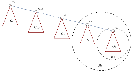
Let {v1,…,vn}\{v_{1},\ldots,v_{n}\} be a path and (G1,v1),…,(Gn,vn)(G_{1},v_{1}),\ldots,(G_{n},v_{n}) disjoined rooted graphs as is shown in Figure 3.
Refer to caption
Figure 3: Path-like cactus

Denote obtained graph by GG and consider it as a rooted graph (G,vn)(G,v_{n}).

Lemma 9

Let G1,G2,…,GnG_{1},G_{2},\ldots,G_{n} be disjoined graphs with specific vertices v1,v2,…v_{1},v_{2},\ldots …,vn\ldots,v_{n} respectively and let GG be the disjoint union of G1,G2,…,GnG_{1},G_{2},\ldots,G_{n}, joined by the edges v1​v2,v2​v3,…,vn−1​vnv_{1}v_{2},v_{2}v_{3},\ldots,v_{n-1}v_{n}. For every i∈{1,…,n}i\in\{1,\ldots,n\}, denote by HiH_{i} the union of graphs G1,…,GiG_{1},\ldots,G_{i}, i.e. Hi=(⋃j=1iGj)∪(⋃j=1i−1(vj,vj+1))H_{i}=\left(\bigcup_{j=1}^{i}G_{j}\right)\cup\left(\bigcup_{j=1}^{i-1}(v_{j},v_{j+1})\right). If i>1i>1, the following is true

γw00​(Hi,vi)\displaystyle\!\!\!\!\!\!\!\gamma_{w}^{00}(H_{i},v_{i}) =\displaystyle\!= γw00​(Gi,vi)+γw​(Hi−1)\displaystyle\!\gamma_{w}^{00}(G_{i},v_{i})+\gamma_{w}(H_{i-1}) (6)
γw1​(Hi,vi)\displaystyle\!\!\!\!\!\!\!\gamma_{w}^{1}(H_{i},v_{i}) =\displaystyle\!= γw1​(Gi,vi)+min⁡{γw1​(Hi−1,vi−1),γw00​(Hi−1,vi−1)}\displaystyle\!\gamma_{w}^{1}(G_{i},v_{i})+\min\big\{\gamma_{w}^{1}(H_{i-1},v_{i-1}),\gamma_{w}^{00}(H_{i-1},v_{i-1})\big\} (7)
γw0​(Hi,vi)\displaystyle\!\!\!\!\!\!\!\gamma_{w}^{0}(H_{i},v_{i}) =\displaystyle\!= min⁡{γw0​(Gi,vi)+γw​(Hi−1),γw00​(Gi,vi)+γw1​(Hi−1,vi−1)}\displaystyle\!\min\big\{\gamma_{w}^{0}(G_{i},v_{i})+\gamma_{w}(H_{i-1}),\gamma_{w}^{00}(G_{i},v_{i})+\gamma_{w}^{1}(H_{i-1},v_{i-1})\big\} (8)
γw​(Hi)\displaystyle\!\!\!\!\!\!\!\gamma_{w}(H_{i}) =\displaystyle\!= min⁡{γw1​(Hi,vi),γw0​(Hi,vi)}.\displaystyle\!\min\big\{\gamma_{w}^{1}(H_{i},v_{i}),\gamma_{w}^{0}(H_{i},v_{i})\big\}\,. (9)

Proof:  Look at the graph HiH_{i} as the disjoint union of subgraphs GiG_{i} and Hi−1H_{i-1} with roots viv_{i} and vi−1v_{i-1} respectively and joined by the edge vi−1​viv_{i-1}v_{i}. These are exactly the assumptions of Lemma 6.

Algorithm 4 PATH-LIKE
Data: a path-like cactus (P,r)(P,r) with the DFS ordered path’s vertices and corresponding parameters γw00\gamma_{w}^{00}, γw1\gamma_{w}^{1}, γw0\gamma_{w}^{0} and γw\gamma_{w} (i.e. WDP and WDN of rooted subgraphs (Gi,vi)(G_{i},v_{i}) as is shown in Figure 3)
set vv is the last vertex in the DFS order;
repeat
w=FATHER⁡(v)w=\mathrm{FATHER}(v);
γw00​(w)=γw00​(w)+γw​(v)\gamma_{w}^{00}(w)=\gamma_{w}^{00}(w)+\gamma_{w}(v);
γw1​(w)=γw1​(w)+min⁡{γw1​(v),γw00​(v)}\gamma_{w}^{1}(w)=\gamma_{w}^{1}(w)+\min\{\gamma_{w}^{1}(v),\gamma_{w}^{00}(v)\};
γw0​(w)=min⁡{γw0​(w)+γw​(v),γw00​(w)+γw1​(v)}\gamma_{w}^{0}(w)=\min\{\gamma_{w}^{0}(w)+\gamma_{w}(v),\gamma_{w}^{00}(w)+\gamma_{w}^{1}(v)\};
γw​(w)=min⁡{γw1​(w),γw0​(w)}\gamma_{w}(w)=\min\{\gamma_{w}^{1}(w),\gamma_{w}^{0}(w)\};
v=wv=w;
until v=rv=r.
Result: γw∗​(P,r)=γw∗​(v)\gamma_{w}^{*}(P,r)=\gamma_{w}^{*}(v)   for   ∗=00,1,0*=00,1,0;
   γw​(P)=γw​(v)\gamma_{w}(P)=\gamma_{w}(v).
Proposition 10 ((Time complexity of PATH-LIKE))

Algorithm PATH-LIKE needs 4​(n−1)4(n-1) additions and 3​(n−1)3(n-1) min\min-operations.

Proof:  By counting all operations in (6), (7), (8) and (9), the proposition follows.

5.2 DD-closed path-like cactus

Let {v1,…,vn}\{v_{1},\ldots,v_{n}\} be a path and (G1,v1),…,(Gn,vn)(G_{1},v_{1}),\ldots,(G_{n},v_{n}) disjoined rooted graphs. We require that both v1v_{1} and vnv_{n} are members of a dominating set. Such a graph GG is drawn on Figure 4.

Refer to caption
Figure 4: D-closed path-like cactus

To calculate the weighted domination parameters and the weighted domination number with the condition that v1∈Dv_{1}\in D, we introduce some additional notation: (for u≠v1u\neq v_{1})

γw,v1​(G)\displaystyle\gamma_{w,v_{1}}(G) =\displaystyle= γw1​(G,v1)\displaystyle\gamma_{w}^{1}(G,v_{1})
γw,v100​(G,u)\displaystyle\gamma_{w,v_{1}}^{00}(G,u) =\displaystyle= γw,v1​(G−u)\displaystyle\gamma_{w,v_{1}}(G-u)
γw,v11​(G,u)\displaystyle\gamma_{w,v_{1}}^{1}(G,u) =\displaystyle= min⁡{w⁡(D)|{u,v1}⊆D}\displaystyle\min\big\{w(D)\,\big|\;\{u,v_{1}\}\subseteq D\big\}
γw,v10​(G,u)\displaystyle\gamma_{w,v_{1}}^{0}(G,u) =\displaystyle= min{w(D)|v1∈D,u∉D}.\displaystyle\min\big\{w(D)\,\big|\;v_{1}\in D,u\notin D\big\}\,.

In the new algorithm for calculating the WDN of a DD-closed path-like cactus we have to provide that the first vertex (v1)(v_{1}) is a member of a dominating set. We apply algorithm PATH-LIKE and make changes in the first step of the loop repeat-until. According to the Figure 3 and Figure 4, that means

γw,v100​(H2,v2)\displaystyle\gamma_{w,v_{1}}^{00}(H_{2},v_{2}) =\displaystyle= γw00​(G2,v2)+γw1​(H1,v1)\displaystyle\gamma_{w}^{00}(G_{2},v_{2})+\gamma_{w}^{1}(H_{1},v_{1}) (10)
γw,v11​(H2,v2)\displaystyle\gamma_{w,v_{1}}^{1}(H_{2},v_{2}) =\displaystyle= γw1​(G2,v2)+γw1​(H1,v1)\displaystyle\gamma_{w}^{1}(G_{2},v_{2})+\gamma_{w}^{1}(H_{1},v_{1}) (11)
γw,v10​(H2,v2)\displaystyle\gamma_{w,v_{1}}^{0}(H_{2},v_{2}) =\displaystyle= γw00​(G2,v2)+γw1​(H1,v1).\displaystyle\gamma_{w}^{00}(G_{2},v_{2})+\gamma_{w}^{1}(H_{1},v_{1})\,. (12)

The other steps do not need corrections and the vertex v1v_{1} on Figure 4 (the last vertex in the DFS order in the algorithm below) on a path remains in a dominating set.

Algorithm 5 DD-CLOSED PATH-LIKE
Data: DD-closed path-like cactus (P,r)(P,r): with DFS ordered path’s vertices and corresponding parameters γw00\gamma_{w}^{00}, γw1\gamma_{w}^{1}, γw0\gamma_{w}^{0} and γw\gamma_{w}, i.e. WDP and WDN of rooted subgraphs (Gi,vi)(G_{i},v_{i})
set vv is the last vertex in DFS order;
l=vl=v;
w=FATHER⁡(v)w=\mathrm{FATHER}(v);
γw00​(w)=γw00​(w)+γw1​(v)\gamma_{w}^{00}(w)=\gamma_{w}^{00}(w)+\gamma_{w}^{1}(v);
γw1​(w)=γw1​(w)+γw1​(v)\gamma_{w}^{1}(w)=\gamma_{w}^{1}(w)+\gamma_{w}^{1}(v);
γw0​(w)=γw00​(w)+γw1​(v)\gamma_{w}^{0}(w)=\gamma_{w}^{00}(w)+\gamma_{w}^{1}(v);
γw​(w)=min⁡{γw1​(w),γw0​(w)}\gamma_{w}(w)=\min\{\gamma_{w}^{1}(w),\gamma_{w}^{0}(w)\};
v=wv=w;
repeat
 w=FATHER⁡(v)w=\mathrm{FATHER}(v);
 γw00​(w)=γw00​(w)+γw​(v)\gamma_{w}^{00}(w)=\gamma_{w}^{00}(w)+\gamma_{w}(v);
 γw1​(w)=γw1​(w)+min⁡{γw1​(v),γw00​(v)}\gamma_{w}^{1}(w)=\gamma_{w}^{1}(w)+\min\{\gamma_{w}^{1}(v),\gamma_{w}^{00}(v)\};
 γw0​(w)=min⁡{γw0​(w)+γw​(v),γw00​(w)+γw1​(v)}\gamma_{w}^{0}(w)=\min\{\gamma_{w}^{0}(w)+\gamma_{w}(v),\gamma_{w}^{00}(w)+\gamma_{w}^{1}(v)\};
 γw​(w)=min⁡{γw1​(w),γw0​(w)}\gamma_{w}(w)=\min\{\gamma_{w}^{1}(w),\gamma_{w}^{0}(w)\};
 v=wv=w;
until v=rv=r.
Result: γw,l∗​(P,r)=γw∗​(v){\gamma}_{w,l}^{*}(P,r)=\gamma_{w}^{*}(v)   for   ∗=00,1,0*=00,1,0;
    γw,l​(P)=γw​(v){\gamma}_{w,l}(P)=\gamma_{w}(v).
Proposition 11 ((Time complexity of DD-CLOSED PATH-LIKE))

Algorithm DD-CLOSED PATH-LIKE needs less than 4​(n−1)4(n-1) additions and 3​(n−1)3(n-1) min\min-operations.

Proof:  In the first step of the algorithm we have 33 additions and one min\min-operation. For the loop we need 4​(n−2)4(n-2) additions and 3​(n−2)3(n-2) min\min-operations.

5.3 Cycle-like cactus

We now consider the case when the specific vertices v1,…,vnv_{1},\ldots,v_{n} in a graph are vertices of a cycle. Let (Cn,vn)(C_{n},v_{n}) be a rooted cycle with vertices v1,…,vnv_{1},\ldots,v_{n} and corresponding weights w1,…,wnw_{1},\ldots,w_{n}, and let (G1,v1),…,(Gn−1,vn−1)(G_{1},v_{1}),\ldots,(G_{n-1},v_{n-1}) be disjoined rooted graphs (in our case cacti). Denote by (Kn,vn)(K_{n},v_{n}) the union of (G1,v1),…(G_{1},v_{1}),\ldots …,(Gn−1,vn−1)\ldots,(G_{n-1},v_{n-1}) and vnv_{n}, joined by the edges v1​v2,v2​v3,…,vn−1​vnv_{1}v_{2},v_{2}v_{3},\ldots,v_{n-1}v_{n} and vn​v1v_{n}v_{1}. Graph (Kn,vn)(K_{n},v_{n}) is depicted in Figure 5.

Refer to caption
Figure 5: Cycle-like cactus

Let (Kn′,vn)(K_{n}^{\prime},v_{n}) be the path-like cactus with specific vertices on the weighted path {vn′,v1,…,vn}\{v_{n}^{\prime},v_{1},\ldots,v_{n}\}, where we additionally define w⁡(vn′)=wnw(v_{n}^{\prime})=w_{n}. Graph (Kn′,vn)(K_{n}^{\prime},v_{n}) is obtained from (Kn,vn)(K_{n},v_{n}) as is shown in Figure 6.

Refer to caption
Figure 6: Graph (Kn′,vn)(K_{n}^{\prime},v_{n}) obtained from (Kn,vn)(K_{n},v_{n})
Lemma 12

For a rooted cycle-like cactus (Kn,vn)(K_{n},v_{n}), the weighted domination parameters and the weighted domination number are the following

γw00​(Kn,vn)\displaystyle\gamma_{w}^{00}(K_{n},v_{n}) =\displaystyle= γw​(Kn−vn)\displaystyle\gamma_{w}(K_{n}-v_{n}) (13)
γw1​(Kn,vn)\displaystyle\gamma_{w}^{1}(K_{n},v_{n}) =\displaystyle= γw,vn′1​(Kn′,vn)−wn\displaystyle\gamma_{w,v_{n}^{\prime}}^{1}(K_{n}^{\prime},v_{n})-w_{n} (14)
γw0​(Kn,vn)\displaystyle\gamma_{w}^{0}(K_{n},v_{n}) =\displaystyle= min⁡{γw1​(Kn−vn,v1),γw1​(Kn−vn,vn−1)}\displaystyle\min\big\{\gamma_{w}^{1}(K_{n}-v_{n},v_{1}),\gamma_{w}^{1}(K_{n}-v_{n},v_{n-1})\big\} (15)
γw​(Kn)\displaystyle\gamma_{w}(K_{n}) =\displaystyle= min⁡{γw1​(Kn,vn),γw0​(Kn,vn)}.\displaystyle\min\big\{\gamma_{w}^{1}(K_{n},v_{n}),\gamma_{w}^{0}(K_{n},v_{n})\big\}\,. (16)

Proof:  Lemma is a direct consequence of the construction of the graph K′K^{\prime}, the definition of γw,vn′1\gamma_{w,v_{n}^{\prime}}^{1} and the properties of the parameters γw0\gamma_{w}^{0} and γw00\gamma_{w}^{00}.

Recall that weighted domination parameters γw00​(Kn,vn)\gamma_{w}^{00}(K_{n},v_{n}), γw1​(Kn,vn)\gamma_{w}^{1}(K_{n},v_{n}) and γw0​(Kn,vn)\gamma_{w}^{0}(K_{n},v_{n}) can be calculated using the previous two lemmas.

Algorithm 6 CYCLE-LIKE
Data: a rooted cycle (C,r)(C,r): with DFS ordered vertices and corresponding parameters γw00\gamma_{w}^{00}, γw1\gamma_{w}^{1}, γw0\gamma_{w}^{0} and γw\gamma_{w}, i.e. WDP and WDN of rooted subgraphs (Gi,vi)(G_{i},v_{i})
set   vv is the last vertex in DFS order;
     rr is the first vertex in DFS order;
     s=ORIEN⁡(v)s=\mathrm{ORIEN}(v);
     l=vl=v;
set new vertex r′r^{\prime} in the DFS table with:
   DFN⁡(r′)=DFN⁡(v)+1\mathrm{DFN}(r^{\prime})=\mathrm{DFN}(v)+1;
   FATHER⁡(r′)=v\mathrm{FATHER}(r^{\prime})=v;
   (MARK⁡(r′)=1\mathrm{MARK}(r^{\prime})=1, ROOT⁡(r′)=r′\mathrm{ROOT}(r^{\prime})=r^{\prime}, ORIEN⁡(r′)=r′\mathrm{ORIEN}(r^{\prime})=r^{\prime}, IND⁡(r′)=1\mathrm{IND}(r^{\prime})=1);
   γw00​(r′)=γw00​(r)\gamma_{w}^{00}(r^{\prime})=\gamma_{w}^{00}(r), γw1​(r′)=γw1​(r)\gamma_{w}^{1}(r^{\prime})=\gamma_{w}^{1}(r), γw0​(r′)=γw0​(r)\gamma_{w}^{0}(r^{\prime})=\gamma_{w}^{0}(r) and γw​(r′)=γw​(r)\gamma_{w}(r^{\prime})=\gamma_{w}(r).
calculate
  1. ∙\bullet

    γw​(C−r)\gamma_{w}(C-r) and γw1​(C−r,s)\gamma_{w}^{1}(C-r,s) using PATH-LIKE on DFS ordered path’s vertices {s,…,v}\{s,\ldots,v\}

  2. ∙\bullet

    γw,r′1​(C∪{r′},r){\gamma}_{w,r^{\prime}}^{1}(C\cup\{r^{\prime}\},r) using D-CLOSED PATH-LIKE on DFS ordered path’s vertices {r,s,…,v,r′}\{r,s,\ldots,v,r^{\prime}\}

  3. ∙\bullet

    γw,v​(C−r){\gamma}_{w,v}(C-r) using D-CLOSED PATH-LIKE (v∈Dv\in D) on DFS ordered path’s vertices {s,…,v}\{s,\ldots,v\}

Result: γw00​(C,r)=γw​(C−r)\gamma_{w}^{00}(C,r)=\gamma_{w}(C-r);
         γw1​(C,r)=γw,r′1​(C∪{r′},r)−γw1​(r)\gamma_{w}^{1}(C,r)={\gamma}_{w,r^{\prime}}^{1}(C\cup\{r^{\prime}\},r)-\gamma_{w}^{1}(r);
         γw0​(C,r)=min⁡{γw1​(C−r,s),γw,v​(C−r)}\gamma_{w}^{0}(C,r)=\min\big\{\gamma_{w}^{1}(C-r,s),{\gamma}_{w,v}(C-r)\big\};
         γw​(C)=min⁡{γw1​(C,r),γw0​(C,r)}\gamma_{w}(C)=\min\big\{\gamma_{w}^{1}(C,r),\gamma_{w}^{0}(C,r)\big\}.
Proposition 13 ((Time complexity of CYCLE-LIKE))


If a cycle CC has nn vertices, the algorithm CYCLE-LIKE needs less than 12​(n−1)12(n-1) additions and 9​(n−1)9(n-1) min\min-operations.

Proof:  Using algorithms PATH-LIKE and D-CLOSED PATH-LIKE we obtain:

  1. ∙\bullet

    For calculating the parameters γw​(C−r)\gamma_{w}(C-r) and γw1​(C−r,s)\gamma_{w}^{1}(C-r,s) using PATH-LIKE algorithm on n−1n-1 vertices, we need 4​(n−2)4(n-2) additions and 3​(n−2)3(n-2) min\min-operations.

  2. ∙\bullet

    For calculating the parameter γ¯w1​(C∪{r′},r)\overline{\gamma}_{w}^{1}(C\cup\{r^{\prime}\},r) using D-CLOSED PATH-LIKE algorithm on n+1n+1 vertices, we need 4​n4n additions and 3​n3n min\min-operations.

  3. ∙\bullet

    For calculating γ¯w​(C−r)\overline{\gamma}_{w}(C-r) using D-CLOSED PATH-LIKE algorithm on n−1n-1 vertices, we need 4​(n−2)4(n-2) additions and 3​(n−2)3(n-2) min\min-operations.

Additionally, at the end of the algorithm, we need one addition and two min\min-operations. Adding up all operations, we confirm

4​(n−2)+4​n+4​(n−2)+1=12​n−15<2​(n−1)4(n-2)+4n+4(n-2)+1=12n-15<2(n-1) (17)

additions and

3​(n−2)+3​n+3​(n−2)+2=9​n−10<9​(n−1)3(n-2)+3n+3(n-2)+2=9n-10<9(n-1) (18)

min\min-operations.

6 Algorithm for weighted domination of cacti

As we indicated in the previous sections, the general algorithm for calculating WDN of a cactus graph can be seen as an upgrade of the algorithm TREE. The input data of the main algorithm is the DFS cactus data structure, which is supplemented by four arrays of the initial values of the parameters γw00\gamma_{w}^{00}, γw1\gamma_{w}^{1}, γw0\gamma_{w}^{0} and γw\gamma_{w} for every vertex. The starting point (vertex) of the algorithm is the last unread vertex in the DFS order. If the last vertex lies on a tree, we proceed like in the algorithm TREE. (Some care must be taken for the root of the tree, to correct its parameters following Lemma 7.) However, if the last vertex lies on a cycle, we have to read and remember all cycle’s vertices. Following Remark 3 and Proposition 4, the algorithm calls itself for rooted subcacti, for which the roots are hinges of the cycle. This forces the hinges to obtain new values of parameters where all subcacti rooted at the hinges are considered. Then the algorithm calls subalgorithm CYCLE-LIKE and applies Lemma 7 to correct the values of the parameters of the root of cycle. The algorithm continues until the last unread vertex in the DFS order is the root of the cactus. Pseudocode is given below (Algorithm 8).

Algorithm 7 CACTUS
Data: A rooted cactus (K,r)(K,r) with DFS ordered vertices in the DFS table;
initialize γw00​(v)=0\gamma_{w}^{00}(v)=0, γw1​(v)=w⁡(v)\gamma_{w}^{1}(v)=w(v), γw0​(v)=∞\gamma_{w}^{0}(v)=\infty and γw​(v)=w​(v)\gamma_{w}(v)=w(v) for every vertex vv in the DFS table;
set vv is the last vertex in the DFS order
  Last=v\mathrm{Last}=v;
while Last≠r\mathrm{Last}\neq r do
if Last\mathrm{Last} does not lie on a cycle then
 repeat
   w=FATHER⁡(v)w=\mathrm{FATHER}(v);
   u=vu=v;
  if (ROOT⁡(w)=w\mathrm{ROOT}(w)=w) and (DFN⁡(w)<DFN⁡(v)−1\mathrm{DFN}(w)<\mathrm{DFN}(v)-1) then
   do CACTUS of the rooted subcactus on vertices in the DFS table
   with DFN=DFN⁡(w),…,DFN⁡(v)−1\mathrm{DFN}=\mathrm{DFN}(w),\ldots,\mathrm{DFN}(v)-1 and the root ww
   (we get new values γw00​(w)\gamma_{w}^{00}(w), γw1​(w)\gamma_{w}^{1}(w), γw0​(w)\gamma_{w}^{0}(w), γw​(w)\gamma_{w}(w))
  end if
   γw00​(w)=γw00​(w)+γw​(v)\gamma_{w}^{00}(w)=\gamma_{w}^{00}(w)+\gamma_{w}(v) ;
   γw1​(w)=γw1​(w)+min⁡{γw1​(v),γw00​(v)}\gamma_{w}^{1}(w)=\gamma_{w}^{1}(w)+\min\{\gamma_{w}^{1}(v),\gamma_{w}^{00}(v)\} ;
   γw0​(w)=min⁡{γw0​(w)+γw​(v),γw00​(w)+γw1​(v)}\gamma_{w}^{0}(w)=\min\{\gamma_{w}^{0}(w)+\gamma_{w}(v),\gamma_{w}^{00}(w)+\gamma_{w}^{1}(v)\};
   γw​(w)=min⁡{γw1​(w),γw0​(w)}\gamma_{w}(w)=\min\{\gamma_{w}^{1}(w),\gamma_{w}^{0}(w)\};
   v=wv=w;
 until (ROOT⁡(v)≠v\mathrm{ROOT}(v)\neq v) or (DFN⁡(v)=0\mathrm{DFN}(v)=0)
else(see next page)
end if
Algorithm 8 CACTUS - Part 2
if Last\mathrm{Last} does not lie on a cycle then see previous page
else
 v=Lastv=\mathrm{Last} ;
 repeat (mark the roots of the cycle and correct WDP and WDN arrays
       of hinges on a cycle)
   w=FATHER⁡(v)w=\mathrm{FATHER}(v);
  if DFN⁡(w)<DFN⁡(v)−1\mathrm{DFN}(w)<\mathrm{DFN}(v)-1 then
   do CACTUS of rooted subcactus on vertices in the DFS table with
   DFN=DFN⁡(w),…,DFN⁡(v)−1\mathrm{DFN}=\mathrm{DFN}(w),\ldots,\mathrm{DFN}(v)-1 and the root ww
   (new values γw∗​(w)\gamma_{w}^{*}(w), ∗=00,1,0*=00,1,0 and γw​(w)\gamma_{w}(w))
  end if
   v=wv=w;
 until v=ORIEN⁡(v)v=\mathrm{ORIEN}(v).
 u=vu=v;
 w=FATHER⁡(v)w=\mathrm{FATHER}(v); (ww is now the root of the cycle)
 Make cycle table:
  C=∅C=\emptyset;
  v=Lastv=\mathrm{Last};
  C=D​F​S​(v)C=DFS(v);
  repeat
  v=FATHER⁡(v)v=\mathrm{FATHER}(v);
  C∪D​F​S​(v)C\cup DFS(v);
  until v=wv=w.
 Do CYCLE-LIKE algorithm on the rooted cycle (C,v)(C,v) with vertices in
 the table CC. We obtain parameters of the cycle CC: γw00​(C,v)\gamma_{w}^{00}(C,v), γw1​(C,v)\gamma_{w}^{1}(C,v),
 γw0​(C,v)\gamma_{w}^{0}(C,v) and γw​(C)\gamma_{w}(C);
 γw00​(w)=γw00​(w)+γw00​(C,v)\gamma_{w}^{00}(w)=\gamma_{w}^{00}(w)+\gamma_{w}^{00}(C,v);
 γw1​(w)=γw1​(w)+γw1​(C,v)−WEIGHT⁡(w)\gamma_{w}^{1}(w)=\gamma_{w}^{1}(w)+\gamma_{w}^{1}(C,v)-\mathrm{WEIGHT}(w);
 γw0​(w)=min⁡{γw0​(w)+γw00​(C,v),γw00​(w)+γw0​(C,v)}\gamma_{w}^{0}(w)=\min\{\gamma_{w}^{0}(w)+\gamma_{w}^{00}(C,v),\gamma_{w}^{00}(w)+\gamma_{w}^{0}(C,v)\} ;
 γw​(w)=min⁡{γw1​(w),γw0​(w)}\gamma_{w}(w)=\min\{\gamma_{w}^{1}(w),\gamma_{w}^{0}(w)\};
end if
 Last\mathrm{Last} is determined by DFN⁡(Last)=DFN⁡(u)−1\mathrm{DFN}(\mathrm{Last})=\mathrm{DFN}(u)-1.
Result: γw∗​(K,r)=γw∗​(w){\gamma}_{w}^{*}(K,r)=\gamma_{w}^{*}(w)   for   ∗=00,1,0*=00,1,0;
    γw​(K)=γw​(w){\gamma}_{w}(K)=\gamma_{w}(w).

Denote by bb the number of blocks i.e. the total number of cycles and grafts.

Proposition 14

Algorithm CACTUS properly calculates the weighted domination number of a cactus.

Proof:  Recall that by definition we have two essential situations. If the current vertex vv is a GG-vertex on a subtree or a root of a cycle, the algorithm CACTUS calculates the WDP and the WDN of the subcactus of all vertices with DFN≥DFN⁡(v)\mathrm{DFN}\geq\mathrm{DFN}(v). In particular, when v=rv=r the algorithm CACTUS calculates the WDP and the WDN of the given cactus and we have

γw​(K)=γw​(r).\displaystyle\gamma_{w}(K)=\gamma_{w}(r)\,. (19)

Below we show that algorithm CACTUS needs less than 12​n+5​b12n+5b additions and 9​n+2​b9n+2b min\min operations and thus prove Theorem 1.

Proof:  (of Theorem 1.) Let B1,…,BbB_{1},\ldots,B_{b} be blocks in the cactus and denote by njn_{j} the number of vertices in the block BjB_{j} for each j=1,…,bj=1,\ldots,b. Since a hinge can be the root of more than one block, the number of hinges is less or equal bb. Therefore, we have the inequality

n1+n2+…+nb−b≤n.n_{1}+n_{2}+\ldots+n_{b}-b\leq n\,. (20)

Since the algorithm requires much more time for a cycle block (in comparison with a graft), we can estiamate that for each block BjB_{j} we need less than 12​(nj−1)12(n_{j}-1) additions and 9​(nj−1)9(n_{j}-1) min\min-operations. Furthermore, 5 additions and 2 min\min-operations are needed for sticking blocks in a hinge. Summing up all operations for all blocks in the cactus, we get

∑j=1b12​(nj−1)+5​b=12​(∑j=1bnj−b)+5​b≤12​n+5​b\sum_{j=1}^{b}12(n_{j}-1)+5b=12(\sum_{j=1}^{b}n_{j}-b)+5b\leq 12n+5b

and

∑j=1b9​(nj−1)+2​b≤9​n+2​b.\sum_{j=1}^{b}9(n_{j}-1)+2b\leq 9n+2b\,.
Remark 15

In the proof above, we have assumed that the DFS data structure of the cactus is given. The reason is that the algorithm for kk-trees [13] assumes the structural information of a partial kk-tree is given. It is however well-known that the DFS algorithm is linear in the number of edges of a graph, which for trees and cactus graphs implies that it is also linear in the number of vertices. More precisely, 4​m4m operations are needed when traversing the graph during DFS that provides the DFS cactus data structure: the DFS search has to be followed by a traversal in the opposite DFS order and, in addition. each cycle has to be traversed two more times to assign the roots and the successors to all vertices of a cycle.

Acknowledgement

This work was supported in part by Slovenian Research Agency ARRS (Grant number P1-0285-0101).

References

  • [1] M. Arcak M (2011) Diagonal stability on cactus graphs and application to network stability analysis, IEEE Trans. Autom. Control 56 2766–2777
  • [2] N. Betzler, R. Niedermeier and J. Uhlmann (2006) Tree decompositions of graphs: Saving memory in dynamic programming, Discrete Optimization 3 220-229
  • [3] B.-M. Boaz, B. Binay and S. Qiaosheng (2005) Efficient algorithms for the weighted 2-center problem in a cactus graph, Algorithms and Computation, 16th Int. Symp., ISAAC 2005 Lecture Notes in Computer Science 3827 693–-703 doi:10.1007/11602613_\_70
  • [4] R. E. Burkard and J. Krarup (1998) A Linear Algorithm for the Pos/Neg-Weighted 1-Median Problem on a Cactus, Computing 60 193–215
  • [5] G. J. Chang (2013) Algorithmic Aspects of Domination in Graphs, Handbook of Combinatorial Optmization 221–282
  • [6] E. Cockayne, S. Goodman and S. Hedetniemi (1975) A linear algoithm for the domination number of a tree, Information Processing Letters 4 41–44
  • [7] P. Dankelmann, D. Rautenbach and L. Volkmann (2002) Weighted domination in triangle-free graphs, Discrete Mathematics 250 233–239
  • [8] B. Elenbogen and J. F. Fink (2007) Distance distributions for graphs modeling computer networks, Discrete Applied Mathematics 155 2007 2612–2624
  • [9] S. T. Hedetniemi and R. C. Laskar (1990) Bibliography and domination in graphs and some basic definitions of domination parameters, Discrete Mathematics 86 257–277
  • [10] S. T. Hedetniemi, R. Laskar and J. Pfaff (1986) A linear algorithm for finding a minimum dominating set in a cactus, Discrete Applied Mathematics 13 287–292
  • [11] Y. Lan, Y. Wang and H. Suzuki (1999) A linear-time algorithm for solving the center problem on weighted cactus graphs, Information Processing Letters 71 205–212
  • [12] K. S. Natarajan and L. J. White (1987) Optimum domination in weighted trees, Information processing letters 7 261–265
  • [13] J. A. Telle and A. Proskurowski (1993) Practical Algorithms on Partial kk-Trees wih an Application to Domination-like Problems, Lecture Notes in Computer Science 709 610–621
  • [14] K. Thulasiraman and M. N. S. Swamy (1992) Graphs: theory and algorithms John Wiley & Sons, Inc.
  • [15] B. Zmazek and J. Žerovnik J (2001) The absolute center problem on weighted cactus graph, SOR ’01 proceedings Lenart, Zadnik Stirn and Drobne Ljubljana: Slovenian Society Informatika, Section for Operational Research 189–194
  • [16] B. Zmazek and J. Žerovnik (2003) Computing the Weighted Wiener and Szeged Number on Weighted Cactus Graphs in Linear Time, Croat. Chem. Acta 76 137–143
  • [17] B. Zmazek and J. Žerovnik (2004) The obnoxious center problem in weighted cactus graphs, Discrete Applied Mathematics 136 377–386
  • [18] B. Zmazek B and J. Žerovnik (2005) Estimating the traffic on weighted cactus networks in linear time Ninth International Conference on Information Visualisation (IV’05) 536–-541 doi:10.1109/IV.2005.48