Nonextensive information theoretical machine

As the representatives of statistical learning and ensemble learning methods respectively, support vector machine (SVM) Cortes & Vapnik (1995) and adaboost Freund & Schapire (1997) have got a lot of success in practice. They can both be classified in the margin-based classification methodology Rosset et al. (2004). From the view of loss function, in SVM, hinge loss is employed as measure to find the maximum margin plane. While in adaboost, exponential loss is used to select and combine weak learners. In terms of regularization, $\ell_{2}$-norm and $\ell_{1}$-norm corresponds to Gaussian prior and Laplace prior Zhu & Xing (2009) respectively and are often used to control the model complexity of SVM. While in the boosting framework, iterative regularization is often used as approximate $\ell_{1}$ regularization Rosset et al. (2004). In terms of data transform, SVM maps data into high dimension by kernel function, while adaboost transforms data as the output of weak learners.

Two interesting questions are whether we can unify the mathematical form of SVM and adaboost in a common framework and whether loss function, regularization method and data transform method can be expressed by a unified mathematical theory. In this paper, we give an attempt under nonextensive information theory (NIT) framework. In complex systems with long-range interaction, long-time memory and multifractals Tsallis (2001), the equilibrium state often shows power-law distribution instead of exponential distribution. Therefore, the well-known Boltzmann distribution (which is exponential distribution) cannot be well used. NIT as a generalization of Shannon information theory aims to model power-law phenomenon by generalizing Boltzmann-Gibbs-Shannon (BGS) entropy to Tsallis entropy of which the maximum entropy distribution is power-law distribution if the entropy index $q\neq 1$.

In machine learning, there has been some applications of Tsallis entropy and its related concepts such as Tsallis mutual information kernel Martins et al. (2009), t-logistic regression Ding & Vishwanathan (2010), approximate inference based on t-divergence Ding et al. (2011). In Martins et al. (2009), Tsallis mutual information kernel is proposed by extending Jensen-Shannon divergence and Shannon entropy to Jensen-Tsallis $q$-difference and Tsallis entropy; in Ding & Vishwanathan (2010), convex loss is extended to nonconvex loss by using $q$-exponential families; in Ding et al. (2011), approximate inference is used to $q$-exponential family by defining a new divergence.

Concretely, our contributions are:

• •

  By using the concepts and methods from NIT, we propose nonextentive information theoretical machine (NITM) to address binary classification task. Its solution and explicit primal and dual formulations are given.

• •

  By observation, we show that all the well-known $\ell_{0/1}$ loss, hinge loss, squared hinge loss and exponential loss are the maximum unnormalized Tsallis entropy distribution with different entropy indices $q$;

• •

  By using Tsallis divergence and $q$-expectation, we show that Gaussian prior ($\ell_{2}$ norm) regularization can be extended to the more general Student-t prior regularization with similar computational complexity.

• •

  By considering the existing work of nonextensive mutual information kernel Martins et al. (2009), we show that all the three parts of discriminative model, e.g., loss function, regularization and data transform can be expressed consistently under the framework of NIT.

• •

  By experiments, it is showed that NITM can improve the generalization performance on different standard datasets by tuning entropy indices properly.

Nonextensive information theory (NIT) has raised a lot of interest in physical community. In this section, we mainly review some necessary concepts from NIT.

For convenience, firstly $q$-exponent and $q$-logarithm Tsallis (2001) are defined as

where $[x]_{+}$ stands for $\max\{x,0\}$ and $\exp_{1}x=\lim_{q\rightarrow 1}\exp_{q}x=\exp x$, $\ln_{1}x=\lim_{q\rightarrow 1}\ln_{q}x=\ln x$. By its definition, one has

Corresponding to the definition of exponential family, one can define $q$-exponential family Amari & Ohara () as

where $\bm{\theta}$ is parameters and $\psi_{q}(\bm{\theta})$ is log normalized factor.

In addition, denote indicator function

Denote the real line and the nonnegative half-line by $\mathbb{R}$ and $\mathbb{R}_{+}$ respectively. The set of $n$-dimensional vectors with positive components of sum $1$ is denoted by

In addition, denote $\mathbf{1}_{n}$ as a vector in $\mathbb{R}_{+}^{n}$ with all elements $1$.

For $\mathbf{p}\in\Delta_{n}$, Tsallis entropy is defined as Tsallis (1988); Tsallis (2001)

where $k$ is an arbitrary positive constant. For convenience, set $k=1$ in the following context. For $q=1$, $S_{1}(\mathbf{p})$ is equivalent to the definition of Shannon entropy. For $q=0$ and $i\in\{1,2,\ldots,n\}$, define $p_{i}^{q}=0$ if $p_{i}=0$ and $p_{i}^{q}=1$ if $p_{i}\neq 0$, then

where $\|\cdot\|_{0}$, called $\ell_{0}$ pseudo norm, denotes the number of nonzero elements in vector. If $q<0$, $S_{q}(p)$ is convex; if $q>0$, $S_{q}(p)$ is concave. In all cases, $S_{q}\geq 0$ (nonnegativity property). For two independent random variables $A$ and $B$, with probability mass function $\mathbf{p}_{A}\in\Delta_{n_{A}}$ and $\mathbf{p}_{B}\in\Delta_{n_{B}}$ respectively, consider the new random variable $A\cup B$ defined by the joint distribution $\mathbf{p}_{A}\cup\mathbf{p}_{B}\in\Delta^{n_{A}n_{B}}$, then Tsallis (1988),

which is called the nonextensive property of Tsallis entropy. One can immediately see that $q<1,q=1$ and $q>1$ respectively correspond to superextensivity (superadditivity), extensivity (additivity) and subextensivity (subadditivity). An axiomatic framework for Tsallis entropy (for all $q\in\mathbb{R}$) and an uniqueness theorem can be seen in dos Santos (1997).

As a measure of similarity on $\mathbb{R}_{+}^{n}$, for $\mathbf{p},{\mathbf{t}}\in\mathbb{R}_{+}^{n}$ and $q\in\mathbb{R}$, generalized Tsallis divergence Martins et al. (2009) is defined as

For $q=1$, $D_{q}(\mathbf{p}\|{\mathbf{t}})$ is the definition of the generalized Kullback-Leibler (KL) divergence Csiszár (1975).

For the case $\mathbf{p},{\mathbf{t}}\in\Delta_{n}$, by the definition of $D_{q}(\mathbf{p}\|{\mathbf{t}})$ in (1), one has

which is called the Tsallis divergence on discrete probability distribution. For $q=1$, $D_{1}(\mathbf{p}\|{\mathbf{t}})$ is the well-known KL divergence.

Similarly, for two unnormalized probability density functions (pdf) $p({\mathbf{x}})$ and $t({\mathbf{x}})$ on ${\mathbf{x}}\in\mathbb{R}^{n}$, the generalized Tsallis divergence can be defined as

For normalized pdfs $p({\mathbf{x}})$ and $t({\mathbf{x}})$, where $\int p({\mathbf{x}})d{\mathbf{x}}=1,\int t({\mathbf{x}})d{\mathbf{x}}=1$, one has

which is called the Tsallis divergence on continuous probability distribution. Meanwhile, for the normalized pdf $p({\mathbf{x}})$, Tsallis entropy can be defined as

For $q>0$, $D_{q}(p({\mathbf{x}})\|t({\mathbf{x}}))$ is a special case of f-divergence (see Cichocki & Amari (2010) and reference therein), which has the following properties.

• •

  Convexity: $D_{q}(p({\mathbf{x}})\|t({\mathbf{x}}))$ is convex with respect to (w.r.t.) both $p({\mathbf{x}})$ and $t({\mathbf{x}})$;

• •

  Strict Positivity: $D_{q}(p({\mathbf{x}})\|t({\mathbf{x}}))\geq 0$ and $D_{q}(p({\mathbf{x}})\|t({\mathbf{x}}))=0$ if and only if $p({\mathbf{x}})=t({\mathbf{x}})$.

Because of the two useful properties, the value of $D_{q}(p({\mathbf{x}})\|t({\mathbf{x}}))$ with $q>0$ can be used to measure the similarity between $p({\mathbf{x}})$ and $t({\mathbf{x}})$. In practice, one can make $p({\mathbf{x}})$ get close to $t({\mathbf{x}})$ as much as possible by minimizing $D_{q}(p({\mathbf{x}})\|t({\mathbf{x}}))$ w.r.t. $p({\mathbf{x}})$.

The above two properties also hold for $D_{q}(\mathbf{p}\|{\mathbf{t}})$ in the discrete case.

Particularly, in the discrete case, let ${\mathbf{t}}=\frac{1}{n}\mathbf{1}_{n}$, then for $\mathbf{p}\in\Delta_{n}$,

which shows that for a fixed $q$, there exists a one-to-one correspondence between $D_{q}\left(\mathbf{p}\|\frac{1}{n}\mathbf{1}_{n}\right)$ and $S_{q}(\mathbf{p})$. In fact, the entropy of $\mathbf{p}$ can be understood as the degree of similarity from $\mathbf{p}$ to uniform distribution Shore & Johnson (). Therefore, maximizing Tsallis entropy $S_{q}(\mathbf{p})$ is equivalent to minimizing Tsallis divergence $D_{q}\left(\mathbf{p}\|\frac{1}{n}\mathbf{1}_{n}\right)$.

For unnormalized discrete probability distribution $\mathbf{p}$ and $q>0$, $D_{q}\left(\mathbf{p}\|\mathbf{1}_{n}\right)$ is also an effective measure to the distance from $\mathbf{p}$ to the unnormalized uniform distribution $\mathbf{1}_{n}$. Neglecting constants, one can define $-D_{q}\left(\mathbf{p}\|\mathbf{1}_{n}\right)$ as the unnormalized Tsallis entropy of $\mathbf{p}$. Therefore, minimizing $D_{q}\left(\mathbf{p}\|\mathbf{1}_{n}\right)$ can be seen as maximizing unnormalized Tsallis entropy of $\mathbf{p}$. In order to describe the result in Section III consistently, we define $D_{\infty}\left(\mathbf{p}\|\mathbf{1}_{n}\right)$ by its limit given by

Given a set of instance-label pairs $({\mathbf{x}}_{i},y_{i}),$ $i\in\{1,2,\ldots,m\}$, ${\mathbf{x}}_{i}\in\mathbb{R}^{n},y_{i}\in\{-1,+1\}$, $\{\phi_{i}(\cdot)\}_{i=1}^{d}$ is a group of fixed basis functions. Denote $\mathbf{\Phi}=(\bm{\phi}_{1},\bm{\phi}_{2},\ldots,\bm{\phi}_{d})=({\mathbf{f}}_{1},{\mathbf{f}}_{2},\ldots,{\mathbf{f}}_{m})^{T}$, where $\bm{\phi}_{j}=(\phi_{j}({\mathbf{x}}_{1}),\phi_{j}({\mathbf{x}}_{2}),\ldots,\phi_{j}({\mathbf{x}}_{m}))^{T}$ for $j=1,2,\ldots,d$ and ${\mathbf{f}}_{i}=(\phi_{1}({\mathbf{x}}_{i}),\phi_{2}({\mathbf{x}}_{i}),\ldots,\phi_{d}({\mathbf{x}}_{i}))^{T}$ for $i=1,2,\ldots,m$. Nonextensive information theoretical machine (NITM) solves the following constrained problem:

where ${\mathbf{w}}\in\mathbb{R}^{d}$ is assumed to be a continuous random vector with normalized pdf $p({\mathbf{w}})$. Unlike the common $\ell_{2}$-norm or $\ell_{1}$-norm regularization, we impose Bayesian prior $p_{0}({\mathbf{w}})$ on ${\mathbf{w}}$ and use Tsallis divergence

to measure the distance of distribution from the posterior distribution $p({\mathbf{w}})$ to $p_{0}({\mathbf{w}})$. Instead of using the normal expectation Zhu & Xing (2009), $q$-expectation $\int{\mathbf{w}}p^{q}({\mathbf{w}})d{\mathbf{w}}$ in (4) is used Curado & Tsallis (1991). Meanwhile,

can be seen as an unnormalized probability mass distribution (pmf) belonging to $q^{\prime}$-exponential family. The sum $\sum_{i=1}^{m}\exp_{q^{\prime}}(-z_{i})$ is used as loss function. The regularization term and loss function are connected by the constraint of $q$-expectation (4). $C>0$ is the regularization parameter to tune the relative weight of the two terms. $q$ and $q^{\prime}$ are called “entropy indices” in NIT.

Due to the Bayesian-style treatment of ${\mathbf{w}}$, the final output used to give a discriminant to a new data ${\mathbf{x}}$ is the posteriori $q$-expectation, denoted as

and the discriminative function is

It should be noted that $\langle{\mathbf{w}}\rangle_{p^{q}}$ is needed to exist in this paper, but it does not mean the normal expectation $\langle{\mathbf{w}}\rangle_{p}$ exists at the same time.

Setting $q^{\prime}$ to $\{0,1/2\}$ and taking limit at $q^{\prime}\rightarrow-\infty,1$, one has the following result.

From Theorem 1, $\ell_{0/1}$ loss corresponds to $q^{\prime}$-exponential family with $q^{\prime}\rightarrow-\infty$, which is concave. Hinge loss can be seen as the tightest convex relaxation to $\ell_{0/1}$ loss, which is similar to the relationship between $\ell_{1}$-norm and $\ell_{0}$-norm. For $q^{\prime}=\frac{1}{2}$, the coefficient $\frac{1}{2}$ is only a scale factor and the formulation is equivalent to the standard squared hinge loss $[1-z]_{+}^{2}$ after scaling $z$. For $q^{\prime}>1$, as $z\rightarrow(\frac{1}{1-q^{\prime}})^{+}$, $\exp_{q^{\prime}}(-z)\rightarrow+\infty$. Then if one wants the objective function is bounded in any bounded interval, $q^{\prime}=1$, which corresponds to exponential loss, is the largest value we can choose. Therefore, in this paper, $q^{\prime}$ is selected in $[0,1]$.

The general model doesn’t constrain the selection of $q$ and $p_{0}({\mathbf{w}})$, but it is necessary to select them carefully for model effectiveness and computational efficiency. In this paper, Student-t distribution is considered, for its good properties.

• •

  Its support is $\mathbb{R}^{d}$;

• •

  By varying its degrees of freedom $\nu$, it can model the heavy tailed distribution with different thickness;

• •

  Taking $\nu\rightarrow+\infty$, it is equivalent to Gaussian distribution;

The general model (3) couples a variational optimization subproblem and a numerical optimization subproblem together. For $q\geq 1$, $D_{q}(p({\mathbf{w}})\|p_{0}({\mathbf{w}}))$ in (3) and $q$-expectation in (4) are convex w.r.t. $p({\mathbf{w}})$. In addition, for $0\leq q^{\prime}\leq 1$, $\exp_{q^{\prime}}(-z_{i})$ in (5) is also convex. Therefore, for the entropy indices $q\geq 1$ and $0\leq q^{\prime}\leq 1$, the general model is a convex problem w.r.t. $p({\mathbf{w}})$ and ${\mathbf{z}}$. On the one hand, the problem can be solved directly by some variational optimization technique, or convex optimization method if $D_{q}(p({\mathbf{w}})\|p_{0}({\mathbf{w}}))$ and $q$-expectation can be explicitly expressed in terms of distribution parameters. On the other hand, one can solve it indirectly by solving the Lagrange dual problem. Our first main result is about the solution of $p({\mathbf{w}})$ expressed by Lagrange multipliers and the dual optimization formulation of the general model (3).

The posterior distribution $p({\mathbf{w}})$ in (6) is parametrized by dual variables $\bm{\beta}$. The factor $p_{0}^{q-1}({\mathbf{w}})$ in $\exp_{q}(\cdot)$ is emerged by the use of $q$-expectation, which is the key to get a normalizable solution of $p({\mathbf{w}})$. In (7), it shows that minimizing the sum of the unnormalized pmf $\sum_{i=1}^{m}\exp_{q^{\prime}}(-z_{i})$ w.r.t. ${\mathbf{z}}$ under the constraint (4) is equivalent to maximizing the unnormalized Tsallis entropy $-D_{1/q^{\prime}}\left(\bm{\beta}/C\|\mathbf{1}_{m}\right)$ of the scaled dual variables $\frac{\bm{\beta}}{C}$ under the nonnegative constraint $\bm{\beta}>{\mathbf{0}}$. For $q^{\prime}\rightarrow 0^{+}$, i.e., $1/q^{\prime}\rightarrow+\infty$, according to (2),

which is equivalent to the dual formulation of hinge loss Zhu & Xing (2009).

In Zhu & Xing (2009), the authors emphasize the advantage of combing maximum entropy learning with maximum margin learning. However, from our perspective, maximum margin learning is the dual formulation of the maximum unnormalized Tsallis entropy learning. Therefore, maximum entropy learning and maximum margin learning can be unified by the concepts of NIT in the NITM model.

Consider the Student-t prior distribution

where $Z_{0}=\frac{\Gamma(\nu/2)\nu^{d/2}\pi^{d/2}}{\Gamma((\nu+d)/2)}$, $d$ is the dimension of ${\mathbf{w}}$, $\nu>0$ is the degrees of freedom. $\Gamma(\cdot)$ denotes Gamma function. For $\nu>2$, both the mean and covariance of $p_{0}({\mathbf{w}})$ exist and equal ${\mathbf{0}}$ and $\frac{\nu}{\nu-2}{\mathbf{I}}$ respectively.

In order to get an analytic solution, we set

then

In addition, if $\nu$ is expressed by $q$, then

where $Z_{0}$ can be written as

Imposing the above prior distribution $p_{0}({\mathbf{w}})$, the normalization factor $Z_{q}(\bm{\beta})$ can be expressed explicitly. Thus one has the following concrete results.

Similar to $p_{0}({\mathbf{w}})$, $p({\mathbf{w}})$ in (13) is also a Student-t distribution. The variance $c$ is decided uniquely by $\bm{\mu}$ and $\nu$. Optimizing $p({\mathbf{w}})$ is equivalent to updating the paramaters $\bm{\mu}$ of $p_{0}({\mathbf{w}})$ according to (14), which generalizes the conjugate prior property of exponential family. In the dual formulation (15), one can see that (15) generalizes the dual formulation of $\ell_{2}$-norm regularizer by imposing an outer function on $\|{\mathbf{H}}^{T}\bm{\beta}\|_{2}^{2}$.

Based on the solution (13) of $p({\mathbf{w}})$, one can also solve the primal problem directly by simplifying $D_{q}(p({\mathbf{w}})\|p_{0}({\mathbf{w}}))$. For simplicity, we use $\nu$ instead of $q$ in the following results.

From Theorem 4, minimizing Tsallis divergence from $p({\mathbf{w}})$ to $p_{0}({\mathbf{w}})$ w.r.t. $p({\mathbf{w}})$ is equivalent to minimizing a convex numerical optimization problem $\emph{w.r.t.}$ $\bm{\mu}$.

Summarizing the above results, NITM unifies $\ell_{0/1}$ loss, hinge loss, squared hinge loss and exponential loss by unnormalized Tsallis entroy with single parameter $q^{\prime}$. Meanwhile, NITM unifies Gaussian prior and Student-t prior by Tsallis divergence and $q$-expectation with single parameter $q$. Furthermore, NITM unifies loss function and regularization by the concepts of NIT. In Martins et al. (2009), the authors showed nonextensive information theory can also be used in the design of kernel, named Tsallis mutual information kernel. By this framework, they unifies the existed linear kernel, Jensen-Shannon kernel and boolean kernel in one parametric family. Therefore, we have Proposition 1.

Unlike MaxEnDNet in Zhu & Xing (2009) which needs resort to variational approximation, we can directly optimize the dual formulation (15) or the primal formulation (16) based on gradient-based convex optimization. After optimizing $\bm{\beta}$ in (15) or $\bm{\mu}$ in (16), the posterior distribution $p({\mathbf{w}})$ can be acquired in (13).

We illustrate the performance of NITM with Student-t prior (11) on standard datasets. The concrete settings are

• •

  $6$ standard datasets: appendicitis, australian, banana, hepatitis, ionosphere, magic¹¹ 1 Available at http://keel.es/datasets.php. Each dataset is divided into $10$ parts by distribution optimally balanced stratified cross-validation (DOB-SCV) (see Moreno-Torres et al. (2012) and reference therein). $3$ parts of them are used as test dataset, while the other $7$ parts are used in cross validation.

• •

  Feature transform: for nominal features, we transform them into double values according to their number which starts from $1$. Before learning, all the features are normalized with $0$ mean and unit length. In addition, a column with all $1$ are added to the feature matrix to learn a bias parameter. In this paper, the main interest is the influence of regularization and loss function to empirical generalization performance, so the group of basis functions $\{\phi_{i}(\cdot)\}_{i=1}^{d}$ are set as identity matrix.

• •

  Parameter setting: NITM has $3$ parameters, $\nu,q^{\prime}$ and $C$. Since NITM includes the existing hinge loss-based SVM, squared hinge loss-based SVM and exponential loss-bass classifier as special cases, in this paper NITM is treated as a meta model. Instances of NITM with concrete values of pair $(\nu,q^{\prime})$ are treated as different models. Meanwhile, $C$ is treated as an inner hyperparameter of model. For an instance of NITM with given $(\nu,q^{\prime})$, $C$ is selected by $7$-cross validation on the divided $7$ parts of each dataset. Then instances of NITM with selected $C$ are compared by test error on the rest uninfluenced $3$ parts. In experiments, we compare $66$ models with $\nu$ from $\{1,10,10^{2},10^{3},10^{4},+\infty\}$ and $q^{\prime}$ from $\{0,0.1,0.2,0.3,0.4,0.5,0.6,0.7,0.8,0.9,1\}$. The inner hyperparameter $C$ of each model is selected among $\{1,10^{2},10^{4},10^{6},10^{8},10^{10}\}$.

• •

  Algorithms: In experiments, we mainly explore the primal convex optimization method to solve NITM. For the model with $q^{\prime}>0$, the optimization problem in (16) is smooth, and thus BFGS method is employed. For $q^{\prime}=0$, which corresponds to hinge loss, the optimization problem is nonsmooth, therefore subgradient BFGS method Yu et al. (2008) is employed. In addition, backtracking line search is used to get global solution and speeds up the iteration. For each problem, the iteration will be stopped if the number of iterations exceeds $5000$ or the direction vector is orthogonal with gradient vector.

• •

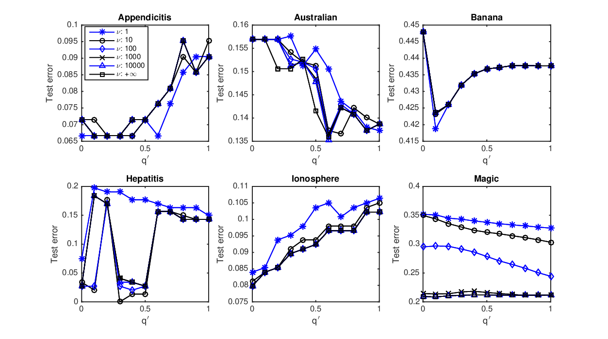
  Result representation: The result is represented in Fig. 1. Each subfigure corresponds to a dataset and reflects the test error as $q^{\prime}$ changes. It deserves to note that for each pair $(\nu,q^{\prime})$, $C$ has been selected in the cross validation stage, so the parameter $C$ of each curve is different in general. The legend on the upper left subfigure is shared among the $6$ subfigures.

In Fig. 1, it is showed that the curves in each subfigure are quite different, which reflects the different physical characteristics of datasets. In order to explain the role of $\nu,q^{\prime}$, the result is analyzed by the order of datasets.

• •

  Appendicitis: It is showed that better performance is acquired when $q^{\prime}$ is relatively small ($q\in\{0,0.1,0.2,0.3,0.4\}$). However, in general, $\nu$ has little influence on test error, except for quite small $\nu=1$, which get smaller test error for many $q^{\prime}\in\{0.6,0.7,0.8\}$ comparing with other values of $\nu$.

• •

  Australian: In general, test error will be small if $q^{\prime}$ is large. For $q^{\prime}=0.6$, the best performance is acquired. For fixed $q^{\prime}$, a large $\nu$ is preferred.

• •

  Banana: The best result will be got when $q^{\prime}=0.1$. Meanwhile, although $\nu$ has little influence, the best test error is got when $\nu=1$.

• •

  Hepatitis: This dataset prefer middle value of $\nu$, e.g, $\nu=10$. The test error will be $0$ if $\nu=10,q^{\prime}=0.3$. In addition, the curve with $\nu=1$ has different shape from that with other $\nu$’s.

• •

  Ionosphere: The consistent shape of the $6$ curves shows that this dataset prefer small $q^{\prime}$ and large $\nu$. The best result is got in the case with $q^{\prime}=0,\nu\rightarrow+\infty$, which corresponds to standard hinge loss-based SVM.

• •

  Magic: This consistent shape shows that large $q^{\prime}$ and large $\nu$ is preferred. Then best result is acquired when $q^{\prime}=1.0,\nu\rightarrow+\infty$, which corresponds to exponential loss with $\ell_{2}$ regularization.

The result shows that different datasets prefer different settings of $(\nu,q^{\prime})$ which is a verification of no-free lunch theorem Wolpert (2002). Although the result seems to be disorder, it is showed that compared with only tuing $C$, tuning $q^{\prime},\nu,C$ independently is not equivalent to tuning $C$ only and can give extra gain of generalization performance.

References

- (1) Amari, Shun-ichi and Ohara, Atsumi. Geometry of q-exponential family of probability distributions. Entropy, 13:1170–1185.
- Cichocki & Amari (2010) Cichocki, Andrzej and Amari, Shun-ichi. Families of alpha-beta-and gamma-divergences: Flexible and robust measures of similarities. Entropy, 12(6):1532–1568, 2010.
- Cortes & Vapnik (1995) Cortes, Corinna and Vapnik, Vladimir. Support-vector networks. Machine learning, 20(3):273–297, 1995.
- Csiszár (1975) Csiszár, Imre. I-divergence geometry of probability distributions and minimization problems. The Annals of Probability, pp. 146–158, 1975.
- Curado & Tsallis (1991) Curado, Evaldo MF and Tsallis, Constantino. Generalized statistical mechanics: connection with thermodynamics. Journal of Physics A: Mathematical and General, 24(2):L69, 1991.
- Ding & Vishwanathan (2010) Ding, Nan and Vishwanathan, SVN. t-logistic regression. In Advances in Neural Information Processing Systems, pp. 514–522, 2010.
- Ding et al. (2011) Ding, Nan, Qi, Yuan, and Vishwanathan, Svn. t-divergence based approximate inference. In Advances in Neural Information Processing Systems, pp. 1494–1502, 2011.
- dos Santos (1997) dos Santos, Roberto JV. Generalization of shannon theorem for tsallis entropy. Journal of Mathematical Physics, 38(8):4104, 1997.
- Freund & Schapire (1997) Freund, Yoav and Schapire, Robert E. A decision-theoretic generalization of on-line learning and an application to boosting. Journal of computer and system sciences, 55(1):119–139, 1997.
- Martins et al. (2009) Martins, André FT, Smith, Noah A, Xing, Eric P, Aguiar, Pedro MQ, and Figueiredo, Mário AT. Nonextensive information theoretic kernels on measures. The Journal of Machine Learning Research, 10:935–975, 2009.
- Moreno-Torres et al. (2012) Moreno-Torres, Jose G, Sáez, José A, and Herrera, Francisco. Study on the impact of partition-induced dataset shift on-fold cross-validation. Neural Networks and Learning Systems, IEEE Transactions on, 23(8):1304–1312, 2012.
- Rosset et al. (2004) Rosset, Saharon, Zhu, Ji, and Hastie, Trevor. Boosting as a regularized path to a maximum margin classifier. The Journal of Machine Learning Research, 5:941–973, 2004.
- (13) Shore, John E. and Johnson, Rodney W. axiomatic derivation of the principle of maximum entropy and the principle of minimum cross-entropy. IEEE transactions on information theory, 1:26–37.
- Teweldeberhan et al. (2005) Teweldeberhan, AM, Plastino, AR, and Miller, HG. On the cut-off prescriptions associated with power-law generalized thermostatistics. Physics Letters A, 343(1):71–78, 2005.
- Tsallis (1988) Tsallis, Constantino. Possible generalization of boltzmann-gibbs statistics. Journal of statistical physics, 52(1-2):479–487, 1988.
- Tsallis (2001) Tsallis, Constantino. I. nonextensive statistical mechanics and thermodynamics: Historical background and present status. In Nonextensive statistical mechanics and its applications, pp. 3–98. Springer, 2001.
- Wolpert (2002) Wolpert, David H. The supervised learning no-free-lunch theorems. In Soft Computing and Industry, pp. 25–42. Springer, 2002.
- Yu et al. (2008) Yu, Jin, Vishwanathan, SVN, Günter, Simon, and Schraudolph, Nicol N. A quasi-newton approach to non-smooth convex optimization. In Proceedings of the 25th international conference on Machine learning, pp. 1216–1223. ACM, 2008.
- Zhu & Xing (2009) Zhu, Jun and Xing, Eric P. Maximum entropy discrimination markov networks. The Journal of Machine Learning Research, 10:2531–2569, 2009.