Point process models for spatio-temporal distance sampling data from a large-scale survey of blue whales

For any subset $A\subseteq\Omega$, the number of objects in $A$ is denoted $N_{\mbox{\boldmath$Y$}}(A)$. For an inhomogeneous point process, we define an intensity function $\Lambda(\mbox{\boldmath$s$})$ as

where $\mathcal{B}_{\epsilon}(\mbox{\boldmath$s$})$ is a ball of radius $\epsilon$ centered at $s$. For all non-overlapping subsets $A_{1},\dots,A_{m}\subset\Omega$, an inhomogeneous Poisson point process has the following two conditions,

Finally, we let $\Lambda(\mbox{\boldmath$s$})$ be a random process, and define the point pattern model conditionally on $\Lambda(\mbox{\boldmath$s$})$. The conditional likelihood for the entire point pattern $Y$, relative to a homogeneous Poisson process with intensity $1$, is given by

where $\mbox{\boldmath$s$}_{i}$ is the location of the $i$th observation. If $\log\Lambda(\mbox{\boldmath$s$})$ is modeled by a latent Gaussian linear model, the resulting hierarchical model is a doubly-stochastic log-Gaussian Cox process (Møller and Waagepetersen,, 2004).

For wildlife surveys, only a proportion of the population in the domain of interest is observed, due to partial sampling of the domain, and failure to detect all animals in the sampled regions. Distance sampling provides a method to account for imperfect detection. In line transect surveys, an observer traces a path through space, searching a strip centered on the path. The probability of detecting an object typically decreases with distance from the observer. From a modeling perspective, this results in a thinned spatial point process with the intensity function scaled by the detection probability (Dorazio,, 2012; Johnson et al.,, 2013; Hefley and Hooten,, 2016).

When deriving the appropriate likelihood model for an observed point pattern, the problem-specific underlying generative structure influences the potential dependence between point locations both over space and in time. It is therefore important to note that the thinning in transect surveys is neither a thinning of a fixed spatial point pattern, nor a thinning of a regular spatio-temporal point process. Instead, each object is characterised by a temporally evolving curve in space, describing its movement, and the observations are thinned snapshots of time-slices of the resulting point process of curves. In addition, the intensity may vary over time, and we write $\lambda(\mbox{\boldmath$s$};t)$ for the spatial point intensity for the full time-slice point pattern at time $t$, and $\Lambda(\mbox{\boldmath$s$};t)$ for the intensity of the observationally thinned version. The assumptions about the movements of the observer and the objects affect what approximations are allowed in practical calculations.

Traditionally, the detection probability for an object located at a given perpendicular distance $z$ from the path of the observer is modeled by a detection function $g(z)$. Assuming that the observer is moving with constant speed $v$ along a straight line, standard Poisson process theory yields the probability of detecting an object located at $\boldsymbol{s}_{0}$ as a function of the perpendicular distance $z(\boldsymbol{s}_{0})$,

where $h(\cdot)$ is an aggregated detection hazard along the path, and $g(\cdot,\cdot)$ is the aggregated detection function, with explicit dependence on $v$. The standard approach is to model either the aggregated detection probability $g(z,v)$, or the aggregated hazard $h(z)$. Under simple assumptions about the observers, Hayes and Buckland, (1983) derived the commonly-used hazard-rate model, given by $h(z)=-(z/\sigma)^{-b}$, $b,\sigma>0$. The half-normal detection function $g(z)=\exp\left[-z^{2}/(2\sigma^{2})\right]$, $\sigma>0$ is another widely-used model. While the hazard-rate model is more flexible than the half-normal detection model, only the latter results in a log-linear probability model. For this reason, the hazard-rate model does not fit directly into the existing INLA estimation software (Rue et al.,, 2009), and instead we use a semi-parametric detection model, which we introduce in Section 3.6, to give us a more flexible model than the half-normal.

For line transects, assuming that environmental and other observational conditions that might affect detectability remain constant along suitably short and straight transect segments, we can formulate a tractably simple version of the likelihood. The region of space swept by the transect path is assumed to consist of a sequence of rectangular transect segment strips $\{\mathcal{C}_{1},\dots,\mathcal{C}_{K}\}$, so that $\mathcal{C}_{k(t)}$ is the transect strip at time $t$. Writing $\lambda(\boldsymbol{s};t)$ for the intensity of potentially observable objects, and introducing transect-dependent detection functions $g_{k(t)}(\mbox{\boldmath$s$})$, the intensity for the thinned observational point process is $\Lambda(\mbox{\boldmath$s$};t)=\lambda(\mbox{\boldmath$s$};t)g_{k(t)}(\mbox{\boldmath$s$})$. Under some loose assumptions (see Supplement A), the joint conditional likelihood for the observed point pattern is the product of the conditional likelihoods for each individual transect segment,

where $N_{\mbox{\boldmath$Y$}}=\sum_{k=1}^{K}N_{\mbox{\boldmath$Y$}}(\mathcal{C}_{k})$ is the total number of observed objects, located at $(\mbox{\boldmath$s$}_{i},t_{i})$, $i=1,\dots,N_{\mbox{\boldmath$Y$}}$. We do not specifically address the issue of marks here (features or quantities associated with detected groups or animals). Marks that do not affect the detection probability can be modeled alongside the object intensity $\lambda(\mbox{\boldmath$s$};t)$, including possible common fixed effects and dependent random effects (Illian et al.,, 2012). However, marks that do affect the detection probability, such as the sizes of groups of animals, require a joint likelihood expression for the extended dimension point process of object locations and their marks, which is a topic for further development.

Following the classical approach for log-Gaussian Cox processes, we let the logarithm of the intensity $\lambda(\mbox{\boldmath$s$};t)$ be a Gaussian process, with linear covariates $\mbox{\boldmath$x$}(\mbox{\boldmath$s$},t)$, and a zero mean additive Gaussian spatial or spatio-temporal random field $\xi(\mbox{\boldmath$s$},t)$ (Møller et al.,, 1998; Møller and Waagepetersen,, 2004; Møller and Waagepetersen,, 2007). For computational efficiency, we use the INLA method for numerical Bayesian inference with Gaussian Markov random fields (Rue et al.,, 2009; Illian et al.,, 2012; Simpson et al.,, 2012), but the general methodology is not tied to a specific inferential framework.

In the likelihood given by (3.2), the log of the thinned intensity is given by

where we assume Gaussian priors for $\beta$, and a Gaussian random field $\xi$. If the logarithm of the detection probability model is linear in its parameters, this results in a joint linear model with latent Gaussian components.

In general, any link function and spatially coherent linear predictor could be used for $\Lambda$. The point process likelihood only requires $\Lambda$ to be well-defined pointwise, and integrable. In practice, the numerical integration schemes used for practical likelihood evaluation (see Section 4) require piecewise continuity and differentiability. Covariates affecting $\lambda(\mbox{\boldmath$s$};t)$ need to be available throughout the transect region for parameter inference, and throughout the domain of interest for spatial prediction. For practical implementation reasons, spatial covariates are projected onto the same computational function space as the latent field $\xi$ (see Section 4.1). Covariates affecting $g_{k}(\mbox{\boldmath$s$})$ need to be available for each transect segment. Within-segment variation in detectability would require a more expensive numerical integration scheme in Section 4.1, equivalent to splitting segments until they were sufficiently short for our assumption of constant detectability within each segment to be fulfilled. As noted at the end of Section 3.3, marks for individuals are currently only allowed if they do not affect the detection probability.

The full model is given by the following hierarchy,

where $\mbox{\boldmath$\beta$}_{g}$ are parameters controlling the detection model, $\theta$ are further model parameters, such as precision parameters for the latent Gaussian variables. Each of the prior densities $\pi(\xi\mid\mbox{\boldmath$\theta$})$, $\pi(\mbox{\boldmath$\beta$}\mid\mbox{\boldmath$\theta$})$, $\pi(\mbox{\boldmath$\beta$}_{g}\mid\mbox{\boldmath$\theta$})$, and $\pi(\mbox{\boldmath$\theta$})$ are controlled by hyperparameters. Note that in some software packages, including INLA, the parameters $\theta$ themselves are referred to as hyperparameters.

For given prior distributions, the goal is to compute the posterior densities for the latent variables, optionally with $\theta$ integrated out:

where $(\xi^{*},\mbox{\boldmath$\beta$}^{*},\mbox{\boldmath$\beta$}_{g}^{*})$ is an arbitrary latent variable state vector. In the INLA method (Rue et al.,, 2009) this is achieved approximately by replacing $\pi(\xi,\mbox{\boldmath$\beta$},\mbox{\boldmath$\beta$}_{g}\mid\mbox{\boldmath$Y$},\mbox{\boldmath$\theta$})$ with various Gaussian or near-Gaussian approximations, and integrating numerically over $\theta$.

The general model construction requires no particular assumptions on how the spatial or spatio-temporal random field $\xi(\mbox{\boldmath$s$},t)$ is modeled or treated computationally. The only requirement is that the model can be written as a latent Gaussian random field in such a way that the model likelihood can be evaluated numerically. In the context of INLA, that means that we need to construct a Gaussian Markov random field representation of the continuous space process. The traditional approach is to discretize space into a lattice and count the number of sighted points in each lattice cell, but here we take an alternative approach that allows us to use the true sighting locations, and to let $\lambda(\mbox{\boldmath$s$};t)$ vary continuously through space. The results from Lindgren et al., (2011) show how to take advantage of the connection between Gaussian Markov random fields of graphs and stochastic partial differential equations in continuous space. Some details of such models are given in Supplement B and the computational implications are discussed in Section 4.1.

As noted in Section 3.2, the hazard-rate model is not a log-linear model, which means that estimating the parameters does not directly fall under the latent Gaussian model framework of the INLA estimation software (Rue et al.,, 2009). In contrast, the half-normal detection model is $g_{k}(\boldsymbol{s})=\exp\left[-z_{k}(\boldsymbol{s})^{2}/(2\sigma^{2}_{g,k})\right]$, where $z_{k}(\mbox{\boldmath$s$})$ is the perpendicular distance from $s$ to the $k$th transect line segment, and $\sigma_{g,k}$ are scale parameters. This can be written in log-linear form as $\log\left[g_{k}(\boldsymbol{s})\right]=\beta_{g,k}z^{*}_{k}(\boldsymbol{s})$, where $z^{*}_{k}(\boldsymbol{s})=-z_{k}(\boldsymbol{s})^{2}/2$, and $\beta_{g,k}=1/\sigma^{2}_{g,k}$. To allow more flexibility within the log-linear framework we introduce a semi-parametric piecewise quadratic model for the logarithm of the detection function, based on a one-dimensional version of the SPDE in the previous section.

For ease of presentation, first assume that the detection probability is the same for all transects $k$, so that we can write $G[z(\boldsymbol{s})]=-\log[g_{k}(\boldsymbol{s})]$. The prior distribution for $G(z)$ is then defined by the spline-like stochastic differential equation

where $z_{\text{max}}$ is the maximal detection distance, $\gamma>0$ is a smoothness parameter, and $\mathcal{W}(t)$ is a white noise process. The boundary constraints ensure that the detection probability at distance $z=0$ is $1$, and that the probability is flat near $z=0$.

Let $(0,z_{1},z_{2},\dots,z_{p})$ be breakpoints for piecewise quadratic B-spline basis functions $B_{i}(z)$ (Farin,, 2002), such that $z_{p}=z_{\text{max}}$, with the simplest choice of breakpoints being $z_{i}=iz_{\text{max}}/p$, $i=0,1,\dots,p$. The non-parametric model for $G(z)$ can then be used to construct a finite dimensional model

where the $p$ basis functions only include $B_{i}(\cdot)$ that fulfill the boundary conditions (3.5), as shown in Fig 2.

The joint multivariate Gaussian prior distribution for $(\beta_{1},\dots,\beta_{p})\sim\textrm{N}\left(\boldsymbol{0},\boldsymbol{Q}_{\beta}^{-1}(\gamma)\right)$ is constructed with the same finite element technique that will be used for the spatial SPDE in Section 4.1. For uniform breakpoint spacing, increasing $p$ will make this discrete model converge to the continuous domain model, but for finite $p$ the model is effectively a piecewise quadratic semi-parametric model.

Imposing a monotonicity constraint on $g(z)$ is possible by replacing the basis functions for $G(z)$ with increasing basis functions, and mandating positivity of the $\beta_{i}$ coefficients (Ramsay,, 1988). However, because the latter is currently only implemented in INLA for independent $\beta_{i}$, this is restricted to small $p$, such as 2 or 3, since an independence prior would result in a non-smooth function for larger $p$. An alternative that is feasible when sampling from the posterior distribution is to simply reject all non-increasing samples of $G(z)$. If the data are informative, the smoothing from the prior can in practice be enough to yield monotonic estimates without including an explicit constraint.

Relaxing the assumption that the detection function is the same for all transects is most easily done by adding further linear terms to $\log g_{k}(\boldsymbol{s})$ based on observed or constructed covariates that depend on $k$.

The SPDE/GMRF approach works by replacing the continuous domain stochastic PDE model with a finite dimensional Gaussian Markov random field for basis function weights defined on a triangulation of the domain of interest, such that the sparse precision matrix leads to a good approximation of the continuous space SPDE solutions. Given a triangulation mesh (see the right panel of Fig 1 for the triangulation used for the ETP survey area), Lindgren et al., (2011) define a finite element representation (Brenner and Scott,, 2007) of $\xi$ from (B.1),

where $w_{1},\dots,w_{m}$ are stochastic weights, and $\phi_{j}$, $j=1,\dots,m$, are deterministic piecewise linear basis functions defined for each node on the mesh: $\phi_{j}$ equals $1$ at mesh node $j$ and $0$ in all the other mesh nodes. The weight vector $\mbox{\boldmath$w$}\equiv(w_{1},\dots,w_{m})^{\top}$ is a GMRF with its Markovian properties defined by the mesh structure. It follows that $w$ determines the stochastic properties of (4.1) and $w$ is chosen in a way that the distribution of (4.1) approximates the distribution of the solution to the SPDE (B.1). As shown by Lindgren et al., (2011), for the SPDE in (B.1), the resulting weight distribution is $\mbox{\boldmath$w$}\sim\textrm{N}(\mbox{\boldmath$0$},\mbox{\boldmath$Q$}(\tau,\kappa)^{-1})$, where the sparse precision matrix $\mbox{\boldmath$Q$}(\tau,\kappa)$ is a polynomial in the parameters $\tau$ and $\kappa$, and is obtained through finite element calculations.

The practical implication of this construction is that instead of directly using the covariances from (B.2), which results in dense covariance matrices and high computational cost, $\mathcal{O}(m^{3})$, the SPDE/GMRF approach links the continuous and discrete domains in such a way that the computational cost is reduced to $\mathcal{O}(m^{1.5})$. The computational advantages of GMRFs (Rue and Held,, 2005) is strengthened by using INLA for Bayesian inference (Rue et al.,, 2009). For the case of fully observed log-Gaussian Cox point processes, the in-depth analysis by Simpson et al., (2016) of the combined approximation errors induced by the basis function expansion in combination with the likelihood approximation error shows that the resulting approximate posterior distribution is close to the true posterior distribution. Since the integration scheme in the following section is constructed in the same way, we do not include a detailed approximation error analysis here, but note that the SPDE/GMRF approximation is likely to be the largest source of approximation error. Point patterns are relatively uninformative about the latent intensity, which has the practical effect that the realizations of the fields in the posterior distribution are typically smoother than in directly observed process problems. Hence, the approximation error is very small as long as the triangle mesh edges are short compared with the spatial scales of the covariates and of the point pattern intensity variability.

Combining the general distance sampling point pattern likelihood (3.2) with the log-linear model structure for $\Lambda(\mbox{\boldmath$s$};t)$ from (3.3) results in a log-likelihood for the observed point pattern,

where the first term evaluates the log-intensity at the observed locations, and the second term integrates the intensity over the sampled transect segments. The log-likelihood (4.2) is in general analytically intractable as it requires integrals of the exponential of a random field. Therefore, we use numerical integration to evaluate (4.2), and the remainder of this section describes an integration scheme to approximate the integrals efficiently. As noted in Section 3.4, we assume that the covariates $x(\mbox{\boldmath$s$},t)$ are expressed using the same piecewise linear basis functions as $\xi$. For cases where a covariate has a much finer resolution than the one needed for $\xi$, the efficient integration scheme developed here is not appropriate, and further research is needed to develop an integration method that can deal with that without incurring a high computational cost.

For distance sampling surveys, transect areas describe subsets of the earth’s surface. The most natural representation of transect areas would therefore be subsets $\mathcal{C}_{k}\subseteq\mathbb{S}^{2}$ of the sphere, leading to surface integration in the Poisson process likelihood. However, the small scale at which earthbound observers are capable of probing their environment lends itself to easily justifiable simplifications of the numerical integration. Apart from environmental conditions such as the weather, the curvature of the earth puts an upper bound on the distance at which an observer with a given elevation can actually detect an animal. We therefore approximate the surface integrals over $\mathcal{C}_{k}\subset\mathbb{S}^{2}$ by integrals over $\widetilde{\mathcal{C}}_{k}\subset\mathbb{R}^{2}$,

where we use a transect-specific parameterization $\mbox{\boldmath$u$}_{k}$ at coordinate $l$ along and distance $z$ to the transect line, respectively. If $R$ is the radius of the earth, then the Jacobian is $\cos(z/R)$, which gives an approximation error of a factor less than $5\cdot 10^{-6}$ even in the extreme and unrealistic case of an observer at $31$ metres above a calm sea looking at the horizon $20$ kilometres away.

Another fact that we can utilize is that the detection function $g$ does not depend on the position of the observer along the line but only on the distance of an observation from the line. Similarly, if the transect line is narrow compared to the spatial rate of change in the intensity function, we can substitute the evaluation of $\lambda$ by an evaluation at the center of the transect line, $\widehat{z}=0$ (see Fig 3). That is,

together with an arbitrary coordinate $\widehat{l}$ along the transect line.

We can also make use of the fact that $\lambda$ lives on a mesh. If the mesh triangles are small enough, the log-linear function $\lambda(\cdot)$ is approximately linear within each triangle. By splitting a transect line $\mathcal{C}_{k}$ into segments $\mathcal{C}_{k,j},\,j\in 1,\dots,J$, each of which resides in a single triangle (see Fig 3), we obtain a Gaussian quadrature method of order one,

Here, $l_{k,j}$ is half of segment $j$’s length $w_{k,j}$. The integration over the distance parameter can now be approximated by a quadrature rule with an equidistant scheme, so that

where $\widetilde{w}_{k,j}=\frac{2z_{\textrm{max}}}{R}w_{k,j}$ with maximal detection distance $z_{\textrm{max}}$, and we substitute $\widehat{l}=l_{k,j}$. We can then write

where $\mbox{\boldmath$u$}_{k,j,r}$ are points on the perpendicular line through the midpoint of transect k’s segment $j$, and $\widetilde{\mbox{\boldmath$u$}}_{k,j,r}$ is the midpoint of each subsegment line.

As a last step we can again make use of the assumption that the function we are integrating over is approximately linear within a given triangle. It is straightforward to show (see Supplement C) that this means that each integration point can be expressed by an evaluation of the function at the triangle vertices weighted by the within-triangle Barycentric coordinates of the original point (Farin,, 2002). We can therefore summarize integration points that reside in the same triangle and share a common time coordinate $t_{k}$ to such evaluations at the mesh vertices, illustrated in Fig 3. This can, depending on the problem structure, lead to a significant reduction in the respective computational workload.

The approximation error from treating the log-linear function within each triangle as linear can be reduced by subdividing each triangle into four. However, evaluating the function at the mid-points of the original triangle edges as well as the original vertices leads to an increase in the computational cost of at least a factor of four, since the number of edges is approximately three times the number of vertices in the mesh.

We use the above methods to predict the blue whale group density over the ETP survey area for the each of the survey years, and to study the effect of sea surface temperature (SST) on the blue whale group density. The function of interest for density estimation is the intensity of the point process before thinning, denoted $\lambda(\mbox{\boldmath$s$},t)$ in (3.3), which we refer to as the group density.

These data have been analyzed before: Forney et al., (2012) used GAMs to estimate encounter rate, with a two-stage estimation approach and gridded data (counts of detections within small segments of transects). Pardo et al., (2015) also used gridded data, modelling log density in each grid cell as a polynomial function of the absolute dynamic topography, a spatially referenced variable that indicates vertical transport of nutrients and thus productivity. While they included a random component in their density model, it had no spatial structure, assuming independent residuals among grid cells. They estimated all model parameters simultaneously in a hierarchical Bayesian framework. Two key differences between their and our model structures are that we use the ungridded data (i.e. the point locations of each detection rather than counts in user-defined grid cells) in our analysis, and we use a spatially structered Gaussian random field to capture spatial variation in density that is not explained by the observed explanatory variable.

Because the blue whale group size is small (mean of 1.8 and standard deviation 2.1) and the size is easily established, it is realistic to treat the group size of blue whales as known without error (Gerrodette et al.,, 2002). We assume that the group size does not affect the detection probability. The detection of cetaceans on ship surveys also depends on wind conditions, but this is less important for blue whales because of their large body size and conspicuous blows. Therefore, we assume the detection probability depends only on the perpendicular distance for the blue whales in the ETP survey. In our analysis, we truncate the data at perpendicular distance $w=6$ km. We also assume that distances were observed without error for each detected animal group and we fit a semi-parametric model given by (3.6) to estimate the detection function.

To build a spatio-temporal model using the SPDE approach described in Section 4.1, we start by constructing a mesh for the ETP survey as shown in Fig 1. The ETP survey is bounded partially by the coastline and partially by the red line of Fig 1. We use a simplified representation of the actual coastline as the mesh boundary to incorporate the boundary effect because a physical boundary such as the coastline has a strong effect – in this case, there will be no blue whales on land. We use a simplified representation of the coastline, because the actual coastline is too ‘angular’ and hence problematic for the SPDE approach (Lindgren and Rue,, 2015). Meanwhile, we extend the boundary further in the northwest and south directions in the Eastern Tropical Pacific, to exclude the boundary effect for the part of the survey area that is bounded by the red line in Fig 1. Given the low sighting rate of the blue whales, there is little information contained in the data to fit a complicated spatio-temporal stochastic process for the random field, such as the AR(1) temporal process used by Cameletti et al., (2012); even the simpler version of the spatio-temporal process with replicated spatial field over time is not feasible.

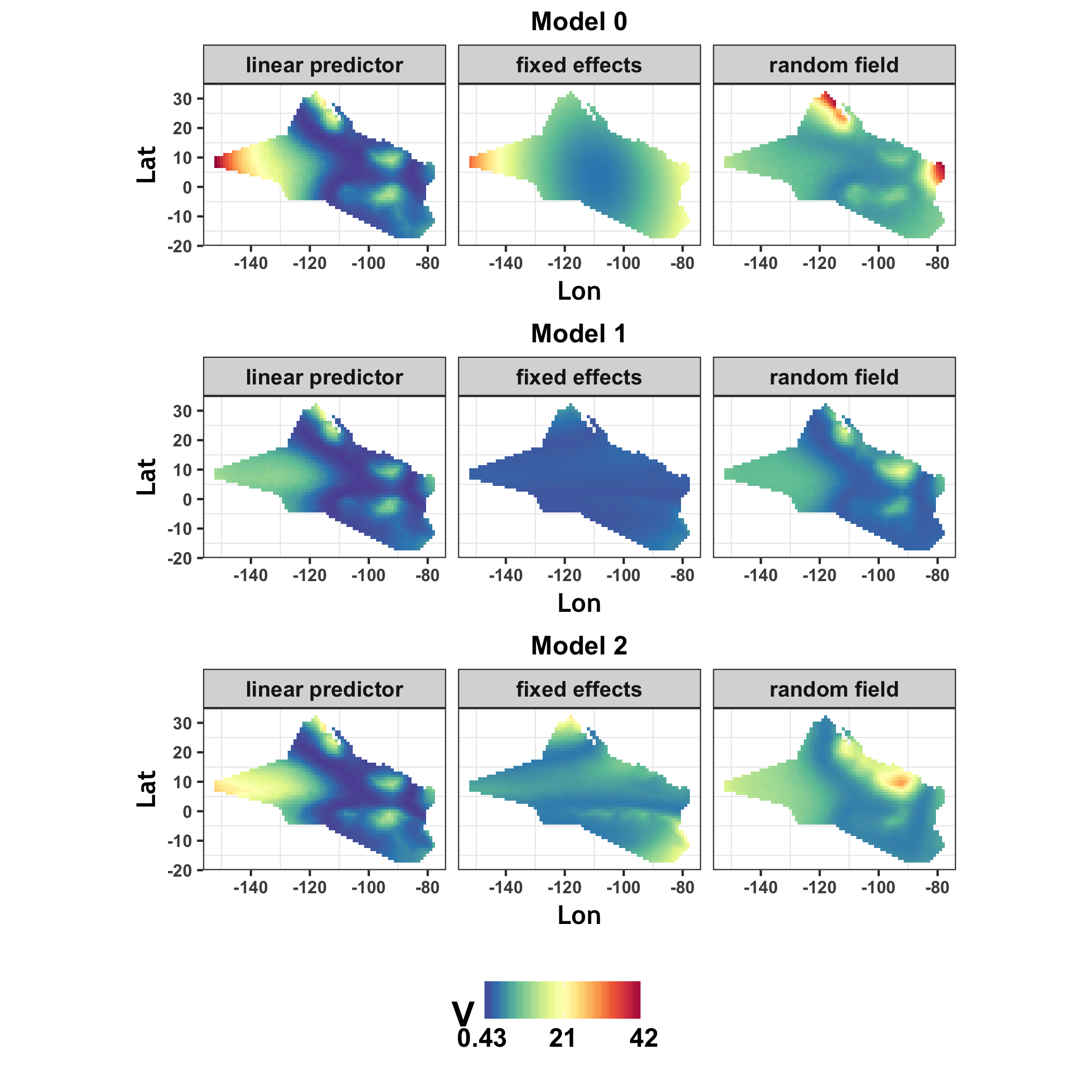
We consider three models, all with Gaussian random fields in space alone. Model 0 has latitude and longitude fixed effects but ignores SST. Model 1 has a temporal SST fixed effect together with spatial residual SST fixed effects for each year. Model 2 has a temporal SST fixed effect and a spatial SST fixed effect together with spatio-temporal residual SST fixed effects.

Based on the Simple Ocean Data Assimilation (SODA) model (http://apdrc.soest.hawaii.edu/datadoc/soda_2.2.4.php), the SST data are available on a fine grid over the ETP survey area on a monthly scale between 1986 and 2007. First, within each year, SST is averaged over the months July to December, during which the survey was conducted. Second, these temporally averaged SST values are spatially smooth, and can be projected onto the mesh of the survey area with only minor loss of fine-scale information. Piecewise linear interpolation is used to calculate the SST for any given location and year, denoted by $\textrm{sst}(\mbox{\boldmath$s$},t)$.

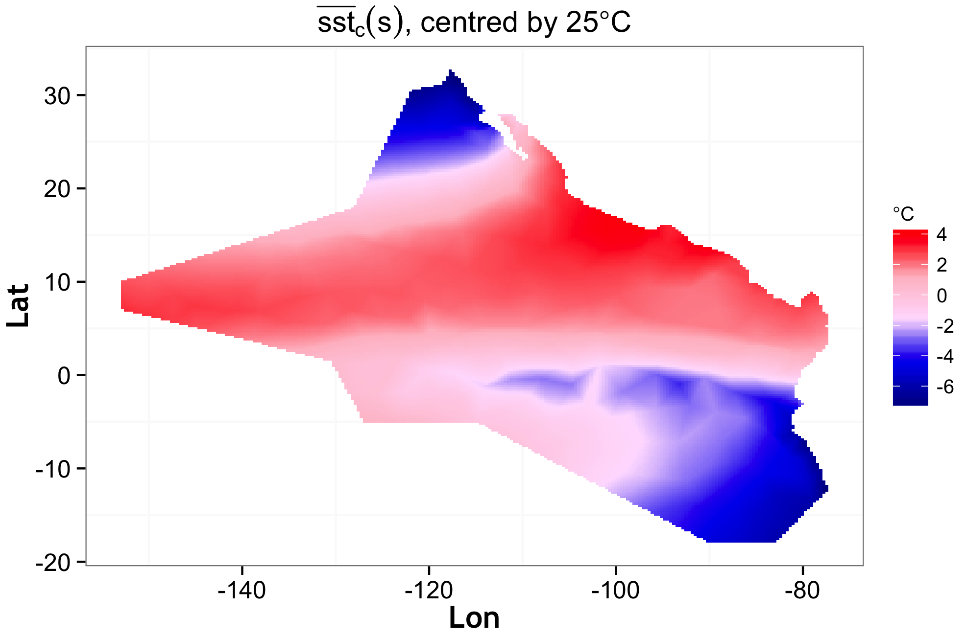
Fig 4 shows the centered SST averaged over time and the centered SST averaged over space. There is both spatial and inter-year variation in SST, and we use hierarchical centering to separate the annual and spatial effects of SST.

Hierarchical centering is a commonly used technique in multilevel modeling (Kreft et al.,, 1995), and we consider two different centering schemes for SST here. Model 0 does not incorporate SST, Model 1 incorporates SST using within-year centering, and Model 2 uses space-time centering. They all have the same SPDE specification of the latent spatial Gaussian random field.

1. 1.

   Model 1: within-year centering. This model has two SST components, the spatially averaged SST for each year, and the spatial SST patterns centered within each year. Let $\Omega$ denote the bounded ETP survey area in Fig 1. We use $\overline{\textrm{sst}}_{c}(t)$ to denote the SST averaged over the ETP survey area for year $t$ after centering,

   $\displaystyle\overline{\textrm{sst}}_{c}(t)$

   $\displaystyle=\frac{1}{|\Omega|}\int_{\Omega}\textrm{sst}(\mbox{\boldmath$s$},t){\,{\mathrm{d}}}\mbox{\boldmath$s$}-\overline{\textrm{sst}},$

   (5.1)

   where $\overline{\textrm{sst}}$ denotes the overall average of SST, $\overline{\textrm{sst}}=\int_{\Omega\times\mathbb{T}}\textrm{sst}(\mbox{\boldmath$s$},t){\,{\mathrm{d}}}\mbox{\boldmath$s$}{\,{\mathrm{d}}}t\big/(|\Omega|\times|\mathbb{T}|)$, with $\mathbb{T}$ denoting the set of survey years. Then the SST centered within year $t$ for location $s$, $\textrm{sst}_{cwy}(\mbox{\boldmath$s$},t)$, is defined as

   $\displaystyle\textrm{sst}_{cwy}(\mbox{\boldmath$s$},t)$

   $\displaystyle=\textrm{sst}(\mbox{\boldmath$s$},t)-\overline{\textrm{sst}}_{c}(t).$

   (5.2)

2. 2.

   Model 2: space-time centering. This model separates the spatial and temporal patters from a spatio-temporal interaction and has three SST components. These are the $\overline{\textrm{sst}}_{c}(t)$ given by (5.1), the SST averaged over years for each location, $\overline{\textrm{sst}}_{c}(\mbox{\boldmath$s$})$ given by (5.3), and the SST residuals, $\textrm{sst}_{res}(\mbox{\boldmath$s$},t)$ given by (5.4),

   	$\displaystyle\overline{\textrm{sst}}_{c}(\mbox{\boldmath$s$})$	$\displaystyle=\frac{1}{|\mathbb{T}|}\int_{\mathbb{T}}\textrm{sst}(\mbox{\boldmath$s$},t){\,{\mathrm{d}}}t-\overline{\textrm{sst}},$		(5.3)
   	$\displaystyle\textrm{sst}_{res}(\mbox{\boldmath$s$},t)$	$\displaystyle=\textrm{sst}(\mbox{\boldmath$s$},t)-\overline{\textrm{sst}}_{c}(t)-\overline{\textrm{sst}}_{c}(\mbox{\boldmath$s$})-\overline{\textrm{sst}}.$		(5.4)

   $\overline{\textrm{sst}}_{c}(t)$ indicates whether a year is relatively warm or cold after averaging over the survey area, and similarly, $\overline{\textrm{sst}}_{c}(\mbox{\boldmath$s$})$ indicates whether a location is relatively warm or cold after averaging over the survey years. The SST residual, $\textrm{sst}_{res}(\mbox{\boldmath$s$},t)$, contains information about the interaction between temporal pattern and the spatial average of SST.

Plots of raw and centered SST used in the analysis are given in Supplement D.

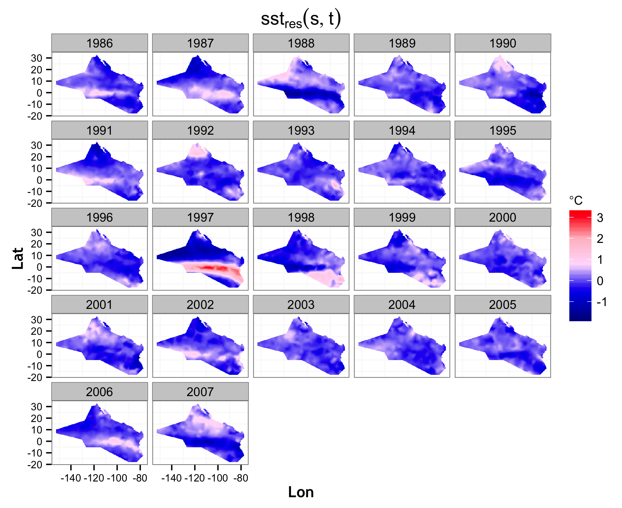
La Niña conditions are characterized by a band of cooler waters in 1988, 1999 and 2007, and El Niño conditions by a much wider band of warm ocean water in 1997 (Wolter and Timlin,, 2011, 1987 is a moderately strong El Niño year according to the scale by). Centering SST strongly captures the El Niño/La Niña oscillations that occur at irregular intervals in the ETP survey area (see Supplement D for more detail). The temporal effect of SST after centering using (5.1) (see Fig 4) correctly reflects the La Niña conditions in 1988 and 2007, and strongly highlights the El Niño year 1997 as an outlier. Unfortunately, no survey was conducted in 1997. Given the time series of $\overline{\textrm{sst}}_{c}(t)$ for the survey years and non-survey years in the right panel of Fig 4, it is obviously problematic to predict for 1997 using a model fitted on the data from the survey years, which are represented by the filled circles in Fig 4. Therefore, we make predictions for all years except 1997.

Table 1 summarizes the posterior density of the regression coefficients for each model.

Let $\eta({\mbox{\boldmath$s$}},t)$ denote the log-intensity defined by the fixed effects and random field components of (3.3),

To investigate the role of the components and the possibility of confounding, we consider the variability around the posterior mean of the overall averages of $\eta({\mbox{\boldmath$s$}},t)$;

and similarly for the components, so that $M_{\eta}=M_{\beta}+M_{\xi}$. The posterior expected squared deviation of $\eta({\mbox{\boldmath$s$}},t)$ from $M_{\eta}$ can be split into contributions from the fixed effects $\mbox{\boldmath$x$}({\mbox{\boldmath$s$}},t)^{\top}\mbox{\boldmath$\beta$}$ and the random field $\xi({\mbox{\boldmath$s$}},t)$;

For all models, $\xi({\mbox{\boldmath$s$}},t)$ is constant over time, and we define the averages across time, $V_{\eta}({\mbox{\boldmath$s$}},\mathbb{T})$, $V_{\beta}({\mbox{\boldmath$s$}},\mathbb{T})$, and $V_{\xi}({\mbox{\boldmath$s$}},\mathbb{T})$, shown in Fig 9 for Model 1 and in Supplement H for all models. It is clear that the random field component $\xi({\mbox{\boldmath$s$}})$ captures information not available in the SST components.

The full space-time averages $V_{\eta}(\Omega,\mathbb{T})$, $V_{\beta}(\Omega,\mathbb{T})$, and $V_{\xi}(\Omega,\mathbb{T})$ are the variances when probing the posterior distributions at a uniformly chosen random locations on $\Omega\times\mathbb{T}$. The remainder term $C_{\beta,\xi}(\Omega,\mathbb{T})$ is the posterior covariance between the fixed effect and random field contributions to the variability. We also define the corellation $\rho_{\beta,\xi}(\Omega,\mathbb{T})=C_{\beta,\xi}(\Omega,\mathbb{T})/\sqrt{V_{\beta}(\Omega,\mathbb{T})V_{\xi}(\Omega,\mathbb{T})}$. A large negative value for the covariance or correlation indicates confounding. Table 2 shows the space-time averages, covariance and correlation for the three models. The correlations are not very small, suggesting that there is some confounding, although it is not severe. While these diagnostics do not give direct guidance for model selection, they highlight the clear contribution of the random field component of each model.

References

- Bailey et al., (2009) Bailey, H. B., Mate, B. R., Palacios, D. M., Irvine, L., Bograd, S. J., and Costa, D. P. (2009). Behavioural estimation of blue whale movements in the Northeast Pacific from state-space model analysis of satellite tracks. In Endangered Species Research, volume 10, pages 93–106.
- Borchers et al., (1998) Borchers, D. L., Buckland, S. T., Goedhart, P. W., Clarke, E. D., and Hedley, S. L. (1998). Horvitz-Thompson estimators for double-platform line transect surveys. Biometrics, 54:1221–1237.
- Borchers and Efford, (2008) Borchers, D. L. and Efford, M. G. (2008). Spatially explicit maximum likelihood methods for capture-recapture studies. Biometrics, 64:377–385.
- Brenner and Scott, (2007) Brenner, S. C. and Scott, L. R. (2007). The Mathematical Theory of Finite Element Methods. Springer, New York, 3rd edition.
- Buckland et al., (2001) Buckland, S. T., Anderson, D. R., Burnham, K. P., Laake, J. L., Borchers, D. L., and Thomas, L. (2001). Introduction to Distance Sampling: Estimating Abundance of Biological Populations. Oxford University Press, Oxford, UK, 1st edition.
- (6) Buckland, S. T., Oedekoven, C. S., and Borchers, D. L. (2015a). Model-based distance sampling. Journal of Agricultural, Biological, and Environmental Statistics.
- Buckland et al., (2016) Buckland, S. T., Oedekoven, C. S., and Borchers, D. L. (2016). Model-based distance sampling. Journal of Agricultural, Biological and Environmental Statistics, 21(1):58–75.
- (8) Buckland, S. T., Rexstad, E. A., Marques, C. S., and Oedekoven, C. S. (2015b). Distance sampling: methods and applications. Springer.
- Cameletti et al., (2012) Cameletti, M., Lindgren, F., Simpson, D., and Rue, H. (2012). Spatio-temporal modeling of particulate matter concentration through the SPDE approach. Advances in Statistical Analysis, 97(2):109–131.
- Conn et al., (2012) Conn, P. B., Laake, J. L., and Johnson, D. S. (2012). A hierarchical modeling framework for multiple observer transect surveys. PLoS ONE, 7(8).
- Cressie et al., (2009) Cressie, N., Calder, C. A., Clark, J. S., Ver Hoef, J. M., and Wikle, C. K. (2009). Accounting for uncertainty in ecological analysis: the strengths and limitations of hierarchical statistical modeling. Ecological Applications, 19:553–570.
- Cressie, (1993) Cressie, N. A. C. (1993). Statistics for Spatial Data. New York: John Wiley & Sons.
- Diggle, (2003) Diggle, P. J. (2003). Statistical Analysis of Spatial Point Patterns. Hodder Arnold, London, 2nd edition.
- Dorazio, (2012) Dorazio, R. M. (2012). Predicting the geographic distribution of a species from presence-only data subject to detection errors. Biometrics, 68:1303–1312.
- Farin, (2002) Farin, G. E. (2002). Curves and surfaces for CAGD: a practical guide. Academic Press, 5th edition.
- Forney et al., (2012) Forney, K. A., Ferguson, M. C., Becker, E. A., Fiedler, P. C., Redfern, J. V., Barlow, J., Vilchis, I. L., and Ballance, L. T. (2012). Habitat-based spatial models of cetacean density in the eastern Pacific Ocean. Endangered Species Research, 16:113–133.
- Gerrodette and Forcada, (2005) Gerrodette, T. and Forcada, J. (2005). Non-recovery of two spotted and spinner dolphin populations in the eastern tropical Pacific Ocean. Marine Ecology Progress Series, 291:1–21.
- Gerrodette et al., (2002) Gerrodette, T., Perryman, W., and Barlow, J. (2002). Calibrating group size estimates of dolphins in the Eastern Tropical Pacific Ocean. Administrative Report LJ-02-08. 20 p.
- Hanks et al., (2015) Hanks, E. M., Schliep, E. M., Hooten, M. B., and Hoeting, J. A. (2015). Restricted spatial regression in practice: geostatistical models, confouding, and robustness under model misspecification. Environmentrics, 26(4):243–254.
- Hayes and Buckland, (1983) Hayes, R. J. and Buckland, S. T. (1983). Radial-distance models for the line-transect method. Biometrics, 39(1):29–42.
- Hedley and Buckland, (2004) Hedley, S. L. and Buckland, S. T. (2004). Spatial models for line transect sampling. Journal of Agricultural, Biological, and Environmental Statistics, 9:181–199.
- Hedley et al., (2004) Hedley, S. L., Buckland, S. T., and Borchers, D. L. (2004). Spatial distance sampling models. In Buckland, S. T., Anderson, D. R., Burnham, K. P., Laake, J. L., Borchers, D. L., and Thomas, L., editors, Advanced Distance Sampling, pages 48–70. Oxford University Press.
- Hefley and Hooten, (2016) Hefley, T. J. and Hooten, M. B. (2016). Hierarchical species distribution models. Current Landscape Ecology Reports, 1:87–97.
- Högmander, (1991) Högmander, H. (1991). A random field approach to transect counts of wildlife populations. Biometrical Journal, 33:1013–1023.
- Högmander, (1995) Högmander, H. (1995). Methods of Spatial statistics in monitoring wildlife populations. University of Jyväskylä, Jyväskylä.
- Illian et al., (2008) Illian, J. B., Penttinen, A., Stoyan, H., and Stoyan, D. (2008). Statistical Analysis and Modelling of Spatial Point Patterns. Wiley, Chichester.
- Illian et al., (2012) Illian, J. B., Sørbye, S. H., and Rue, H. (2012). A toolbox for fitting complex spatial point process models using integrated nested Laplace approximation (INLA). The Annals of Applied Statistics, 6:1499–1530.
- Johnson et al., (2013) Johnson, D. S., Hooten, M. B., and Kuhn, C. E. (2013). Estimating animal resource selection from telemetry data using point process models. Journal of Animal Ecology, 83:1155–1164.
- Johnson et al., (2010) Johnson, D. S., Laake, J. L., and Ver Hoef, J. M. (2010). A model-based approach for making ecological inference from distance sampling data. Biometrics, 66:310–318.
- Johnson et al., (2014) Johnson, D. S., Laake, J. L., and Ver Hoef, J. M. (2014). DSpat: Spatial Modelling for Distance Sampling Data. R package version 0.1.6.
- Kinzey et al., (2000) Kinzey, D., Olson, P., and Gerrodette, T. (2000). Marine Mammal data collection procedures on research ship line-transect surveys by the Southwest Fisheries Science Center. Technical report, National Oceanic and Atmospheric Administration, National Marine Fisheries Service, Southwest Fisheries Science Center.
- Kreft et al., (1995) Kreft, I. G. G., de Leeuw, J., and Aiken, L. S. (1995). The effect of different forms of centering in hierarchicallinear models. Multivariate Behavioural Research, 30:1–21.
- Lindgren and Rue, (2015) Lindgren, F. and Rue, H. (2015). Bayesian spatial modelling with R-INLA. Journal of Statistical Software, 63(19).
- Lindgren et al., (2011) Lindgren, F., Rue, H., and Lindström, J. (2011). An explicit link between Gaussian fields and Gaussian Markov random fields: the SPDE approach (with discussion). Journal of the Royal Statistical Society: Series B, 73(4):423–498.
- Miller et al., (2013) Miller, D. L., Burt, M. L., Rexstad, E. A., and Thomas, L. (2013). Spatial models for distance sampling data: recent developments and future directions. Methods in Ecology and Evolution, 4:1001–1010.
- Miller et al., (2014) Miller, D. L., Rexstad, E. A., Burt, M. L., Bravington, M. V., and Hedley, S. L. (2014). dsm: Density surface modelling of distance sampling data. R package version 2.2.5.
- Møller et al., (1998) Møller, J., Syversveen, A. R., and Waagepetersen, R. P. (1998). Log Gaussian Cox processes. Scandinavian Journal of Statistics, 25:451–482.
- Møller and Waagepetersen, (2004) Møller, J. and Waagepetersen, R. P. (2004). Statistical inference and simulation for spatial point processes. Chapman & Hall/CRC, Boca Raton.
- Møller and Waagepetersen, (2007) Møller, J. and Waagepetersen, R. P. (2007). Modern statistics for spatial point processes (with discussion). Scandinavian Journal of Statistics, 34:643–711.
- Moore and Barlow, (2011) Moore, J. E. and Barlow, J. (2011). Bayesian state-space model of fin whale abundance trends from a 1991-2008 time series of line-transect surveys in the California Current. Journal of Applied Ecology, 48:1195–1205.
- Niemi and Fernández, (2010) Niemi, A. and Fernández, C. (2010). Bayesian spatial point process modeling of line transect data. Journal of Agricultural, Biological, and Environmental Statistics, 15:327–345.
- Oedekoven et al., (2013) Oedekoven, C. S., Buckland, S. T., Mackenzie, M. L., Evans, K. O., and Burger, L. W. (2013). Improving distance sampling: accounting for covariates and non-independency between sampled sites. Journal of Applied Ecology, 50:786–793.
- Oedekoven et al., (2014) Oedekoven, C. S., Buckland, S. T., Mackenzie, M. L., King, R., Evans, K. O., and Burger, L. W. (2014). Bayesian methods for hierarchical distance sampling models. Journal of Agricultural, Biological, and Environmental Statistics, 19:219–239.
- Oedekoven et al., (2015) Oedekoven, C. S., Laake, J. L., and Skaug, H. J. (2015). Distance sampling with a random scale detection function. Environmental and Ecological Statistics, 22:725–737.
- Pardo et al., (2015) Pardo, M. A., Gerrodette, T., Beier, E., Gendron, D., Forney, K. A., Chivers, S. J., Barlow, J., and Palacios, D. M. (2015). Inferring cetacean population densities from the absolute dynamic topography of the ocean in a hierarchical Bayesian framework. PLoS ONE, 10(3):e0120727.
- Ramsay, (1988) Ramsay, J. O. (1988). Monotone regression splines in action. Statistical Science, 3(4):425–441.
- Royle et al., (2004) Royle, J. A., Dawson, D. K., and Bates, S. (2004). Modeling abundance effects in distance sampling. Ecology, 85:1591–1597.
- Royle and Dorazio, (2008) Royle, J. A. and Dorazio, R. M. (2008). Hierarchical Modelling and Inference in Ecology. Academic Press, London, UK.
- Royle and Young, (2008) Royle, J. A. and Young, K. V. (2008). A hierarchical model for spatial capture-recapture data. Ecology, 89:2281–2289.
- Rozanov, (1982) Rozanov, A. (1982). Markov Random Fields. Springer-Verlag, New York.
- Rue and Held, (2005) Rue, H. and Held, L. (2005). Gaussian Markov Random Field: Theory and Applications, volume 104 of Monographs on Statistics and Applied Probability. Chapman & Hall, London.
- Rue et al., (2009) Rue, H., Martino, S., and Chopin, N. (2009). Approximate Bayesian inference for latent Gaussian models by using integrated nested Laplace approximations (with discussion). Journal of the Royal Statistical Society: Series B, 71(2):319–392.
- Schmidt et al., (2012) Schmidt, J. H., Rattenbury, K. L., Lawler, J. P., and Maccluskie, M. C. (2012). Using distance sampling and hierarchical models to improve estimates of dall’s sheep abundance. The Journal of Wildlife Management, 76(2):317–327.
- Simpson et al., (2016) Simpson, D., Illian, J. B., Lindgren, F., Sørbye, S. H., and Rue, H. (2016). Going off grid: Computationally efficient inference for log-Gaussian Cox processes. Biometrika.
- Simpson et al., (2012) Simpson, D., Lindgren, F., and Rue, H. (2012). Think continuous: Markovian Gaussian models in spatial statistics. Spatial Statistics, 1:16–29.
- Stoyan, (1982) Stoyan, D. (1982). A remark on the line transect method. Biometrial Journal, 24:191–195.
- Stoyan and Grabarnik, (1991) Stoyan, D. and Grabarnik, P. (1991). Second-order characteristics for stochastic structures connected with Gibbs point processes. Mathematische Nachrichten, 151:95–100.
- van Lieshout, (2000) van Lieshout, M. (2000.). Markov point processes and their applications. Imperial College Press, London.
- Waagepetersen and Schweder, (2006) Waagepetersen, R. and Schweder, T. (2006). Likelihood-based inference for clustered line transect data. Journal of Agricultural, Biological, and Environmental Statistics, 11(3):264–279.
- Whittle, (1954) Whittle, P. (1954). On stationary process in the plane. Biometrika, 41:434–449.
- Whittle, (1963) Whittle, P. (1963). Stochastic processes in several dimensions. Bulletin of the International Statistical Institute, 40:974–994.
- Wiegand and Moloney, (2014) Wiegand, T. and Moloney, K. A. (2014). Handbook of Spatial Point-Pattern Analysis in Ecology. Chapman & Hall/CRC.
- Williams et al., (2011) Williams, R., Hedley, S. L., Branch, T. A., Bravington, M. V., Zerbini, A. N., and Findlay, K. P. (2011). Chilean blue whales as a case study to illustrate methods to estimate abundance and evaluate conservation status of rare species. Conservation Biology, 25:526–535.
- Wolter and Timlin, (2011) Wolter, K. and Timlin, M. S. (2011). El Niño/Southern Oscillation behaviour since 1871 as diagnosed in an extended multivariate ENSO index (MEI.ext). International Journal of Climatology, 31:1074–1087.
- Wood, (2006) Wood, S. N. (2006). Generalized Additive Models: An introduction with R. Chapman & Hall/CRC, Boca Raton, FL, USA.
A Some assumptions
The assumptions referred to in Section 3.3 are as follows:
- 1.
A team of observers is considered as a joint black box system, and the aggregated detection properties are modeled.
- 2.
Individual objects (animals or animal groups) are not uniquely identified, only their locations are observed.
- 3.
For each segment, the observable regions behind the starting point and ahead of the endpoint are small compared with the length of the segment as a whole, and the partial overlap of segments at changes in path direction is negligible.
- 4.
The time between any other segment overlap is large enough that the time-slice point patterns in the overlap region can be considered independent; the object curves are considered to be in equilibrium, and at least locally mixing faster than the time between revisits by the observer.
B Some details of SPDE models
As noted in the body of the paper, the results from Lindgren et al., (2011) show how to take advantage of the connection between Gaussian Markov random fields of graphs and stochastic partial differential equations in continuous space. The most basic such model is based on the following stochastic partial differential equation (SPDE) defined on a 2-dimensional spatial domain