Predicting the intensity of partially observed data from a revisited kriging for point processes
Abstract
We consider a stationary and isotropic spatial point process whose a realisation is observed within a large window. We assume it to be driven by a stationary random field . In order to predict the local intensity of the point process, , we propose to define the first- and second-order characteristics of a random field, defined as the regularized counting process, from the ones of the point process and to interpolate the local intensity by using a kriging adapted to the regularized process.
Keywords:
Intensity estimation; Point process; Prediction; Spatial statistics.1 Introduction
In many projects the study window is too large to extensively map the intensity of the point process of interest since observation methods may be available at a much smaller scale only. That is for instance the case when studying the spatial repartition of a bird species at a national scale, while the observations are made in windows of few hectares. The intensity must then be estimated from data issued out of samples spread in the study window, and hence, from a partial realisation of the point process in this window.
In the following, we consider a stationary and isotropic point process, , which we assume to be driven by a stationary random field, . We define the local intensity of by its intensity conditional to the random field . We denote it . A simple example of such a process is the Thomas process which is a Poisson cluster process where the cluster centers (parents) are assumed to be Poisson and the offsprings are normally distributed around the parent point. This process is stationary and the local intensity corresponds to the intensity of the inhomogeneous Poisson process of offsprings, i.e. the conditional intensity given the parent process. We will refer to the estimation of the local intensity when we want to the know it at point locations lying in the observation window of the point process, and to its prediction when point locations are outside the observation window.
Usually, when estimating a non-constant intensity, we observe the full point pattern within a window and we want to know its local changes over a given mesh. This issue has been addressed in several ways: kernel smoothing, see [1], [2] in presence of covariates, and [3] for a general class of weight function estimators that encompasses both kernel and tessellation based estimators; or parametric methods; see for instance [4] for a review. A recurrent and remaining question in these approaches is which bandwidth/mesh should we use? This has been addressed by using cross-validation [5] or double kernel [6].
In contrast to the previous methods which look at the intensity changes inside the observation window, our main interest lies in predicting the intensity outside the observation window, all the more when it is not connected as it frequently happens when sampling in plant ecology. To predict the intensity we could use [7]’s reconstruction method based on the first- and second-order characteristics of the point process. Once the empirical point pattern predicted within a given window, one can get the intensity by kernel smoothing. As it is a simulation-based method, it requires long computation times, especially when the prediction window is large and/or the point process is complex. As alternative method, few authors model the point pattern by a point process with the intensity driven by a stationary random field. In [8] and [9], the approach is heavily based on a complete modelling and considers a log-Gaussian model. The parameter estimation, the intensity estimation and its prediction outside the observation window are obtained using a Bayesian framework. The method developed in [10] and [11] is close to classical geostatistics. Basically, it consists of counting the number of points within some grid cells, computing the related empirical variogram and theoretically relating it to the one obtained from the random field driving the intensity. Then, the variogram is fitted and kriging is used to predict the intensity. Its advantage is that the estimation is only based on its first- and second-order moments so that the model does not need to be fully specified. While this approach requires less hypotheses, the model remains constrained within the class of Cox processes. Moreover, the mesh size is arbitrary defined. [12] developed, for a wider class of parametric models, a Bayesian approach for extrapolating and interpolating clustered point patterns.
Here, we propose to interpolate the local intensity by an adapted kriging, where the kriging weights depend on the local structure of the point process. Hence, our method uses all the data to locally predict at a given point, which it is not the case of most of kernel methods. It also uses the information at a fine scale of the point process, which it is not the case in geostatistical approaches. Furthermore, it does not require a specific model but only (an estimation of) the first- and second-order characteristics of the point process.
In Section 2 we define the regularized process as a random field of point counts on grid cells and we link up the mean and variogram of this random field to the intensity and pair correlation function of the point process. The kriging weights, the related interpolator and its properties are presented in Section 3 as well as the optimal mesh of the interpolation grid. In Section 4 we use our kriging interpolator to estimate and predict the intensity of Montagu’s Harriers’ nest locations in a region of France. In Section 5, we discuss the influence of the mesh and the rate and shape of unobserved areas on the statistical properties of our kriging interpolator from numerical results.
2 Linking up characteristics of two theories
2.1 About geostatistics
For any real valued random field , , the first-order characteristic is the mean value function: and the second-order characteristics are classically described in geostatistics [13, 14] by the (semi)-variogram, i.e. the mean squared difference at lag : . For a stationary and isotropic random field, we have
| (1) |
where is the field variance and is the auto-covariance of the random field.
We can interpolate the value at the unsampled location by using the best linear unbiased predictor, so-called kriging interpolator: , where is the observation vector of the random field and is the -vector of weights. In the case of ordinary kriging [15], which will be of interest here since the mean value of the random field will be unknown, we have
| (2) |
where is the covariance matrix between the observations, is the covariance vector between the observations and and is the -vector of 1 (see e.g. [15, 16]).
2.2 About point processes
Let be a stationary and isotropic point process defined in and a Borel set centered at . Following the notations in [17], a realisation of within a window will be denoted by and the random counting measure for a Borel set by .
The first- and second-order characteristics of are described through its intensity and the Ripley’s -function or the pair correlation function :
| (3) | |||||
| (4) | |||||
| (5) |
where is the area of and is the disc centered at , with radius . The intensity is thus the expected number of points per unit area, is the mean number of points in a circle of radius centered at a typical point of the point process, whereas measures how changes with . See for instance [17] for a review about the theory of point processes.
Lemma 2.1
Let be a point process with intensity and , two Borel sets. Then,
- 1.
If , then ,
- 2.
,
- 3.
,
- 4.
If , then .
2.3 Linking up
In our context, data are defined as informative point locations (the realisation of the point process ) while the geostatistical calculations (kriging) need to be carried out over the values of a random field observed at several sampling locations, grid cell centers for example. Thus, we must regularize our process over a compact set [18]. This consists in defining by the count of the point process over the grid cell centered at i.e. . Such a random field is of interest in our case as we want to estimate a non-constant intensity, classically defined by .
From the first- and second-order moments defined in the previous sections, we can link up the characteristics of the point process to the ones of the random field of point counts . Because of the stationary assumption it can also be related to the auto-covariance function (Equation (1)), thus in the following we shall consider the latter.
Proposition 2.2
For the count random field defined by , where is a given Borel set, we have:
- 1.
,
- 2.
For and two regularization blocks, , , ,
- 3.
If , then for
(6)
3 Adapted kriging for point processes
In what follows, we consider that the stationary and isotropic point process, , is driven by a stationary random field, . We want to interpolate the local intensity of , , , i.e. its intensity conditional to the random field , from its realisation within an observation window . Hence, we use the relation between point processes and geostatistics (section 2.3) and approximate the point process by the counting process within a grid of elementary cell .
For sake of clarity, in the following we denote by the region of interest so that define the complementary of within . We consider a regular grid superimposed on with a square-mesh. We denote by an elementary square centered at 0, the elementary square centered at such that , and (resp. ) the number of grid cell centers lying in (resp. ).
3.1 Defining the interpolator
According to the classical geostatistical method defined in Section 2, the kriging interpolator of the local intensity at , , should be written as
for some well-chosen kriging weights where , correspond to data sample locations, i.e. here to the cell centers of . Note that in our case we cannot observe the local intensity at , thus we can estimate it by . Furthermore because of the cell-point relation, we cannot have an exact interpolation of the local intensity.
Proposition 3.1
Given the elementary square , the interpolator at defined by
| (7) |
where , is the best linear unbiased predictor (BLUP) of and the asymptotically BLUP of .
The weights depend on
- 1.
the covariance matrix ,
where , with , and II is the -identity matrix,
- 2.
the covariance vector ,
where , and is the -vector with zero values and one term equals to one where (which only happens in estimation).
When the distance between and , for all , is larger than the range of interaction, the predicted value tends to if and the estimated value tends to 0 if .
Proof: At the scale of , the kriging weights such that is a BLUP of are given by the ordinary kriging equations [15, 19].
At a finer scale we have that tends to when tends to 0 (as is assumed to be continuous). Thus we propose to interpolate by using , with the constraint . Minimising the error variance under this constraint and using Equation (6) lead to the following kriging weights:
where .
To get , note that, for denoting the local intensity of the point process given its realisation in :
and . Thus, we have
- 1.
for ,
which leads to as in our case the local intensity is conditional to the realisation of the process in .
- 2.
for ,
which leads to .
Consequently, and we get
Interpolating or leads to the same kriging weights.
Finally,
shows that is an asymptotically unbiased predictor of .
3.2 Properties of the interpolator
In order to develop the variance of the kriging interpolator, we use the following Neuman series (see e.g. [20]) to invert the covariance matrix , which holds when tends to 0:
| (8) |
where a generic element of the matrix is given by
Proposition 3.2
When tends to 0, the variance of is
| (9) |
In estimation, i.e. when , we get the following approximation,
| (10) |
In prediction, i.e. when , the variance reduces to
| (11) | |||||
Proof: From e.g. [15], the variance of the predictor is given by
When estimating the local intensity, i.e. for lying in the observation window, we have
Thus, from Equation (8):
where ,
and
Then, if is very small, varies in and in . Thus, we get Equation (10).
When predicting the local intensity, i.e. for outside the observation window, we have Thus, from
and
we get Equation (11).
3.3 Defining an optimal mesh size
The Integrated Mean Squared Error of is defined as
When estimating the local intensity, this leads to the following approximation :
| (12) |
We propose to find the optimal mesh of the estimation grid by minimising (see C), and we get :
| (13) |
Note that because the optimal mesh depends on the inverse of squared -norm of the gradient of the local intensity, it decreases for clustered point patterns. Conversely, it increases for regular point patterns.
In practice the optimal mesh can be approximated by estimating the gradient of the intensity over a fine grid (see D).
When predicting the local intensity, the smaller the mesh, the better. Computation time is the only limit.
4 Real case study
In this section we estimate and predict the intensity of Montagu’s Harriers’ nest locations in the Zone Atelier "Plaine & Val de Sèvre"11 1 http://www.za.plainevalsevre.cnrs.fr/ (Figure 1), a NATURA site in France of km2, designated for its remarkable diversity of bird species. Dots in Figure 1 represent the exhaustive collection of Montagu’s Harriers’ nest locations. The area in the center of the Zone Atelier delineates the administrative boundaries of the commune Saint-Martin-de-Bernegoue, which will be used for prediction.

4.1 Estimation of the pair correlation function
The pair correlation is estimated as defined in [21] :
where is the Epanechnikov kernel with bandwidth , the optimal Stoyan’s bandwidth equals to and is the proportion of translations of which have both and inside . Figure 2.a) shows the pair correlation function estimated from either all data point locations (solid line) or only the ones outside the boundaries of Saint-Martin-de-Bernegoue (dashed line). These estimates are characteristic of a Thomas cluster process with an infinite range of correlation, see [4].
4.2 Intensity estimation
For our kriging estimator, the optimal mesh is obtained by minimising the IMSE. Usual nonparametric estimation methods also require to preliminary set the smoothing parameter and this parameter is chosen as an optimal value minimising a specific criterion (typically mean square error, integrated bias, asymptotic mean square error). In our case, we have an explicit formula of the optimal mesh (Equation (13)), which depends on the unknown terms and . If appears to be a natural candidate to estimate , the challenging goal is to estimate . Based on simulation experiments (D), we consider a Gaussian kernel [1], with a bandwidth minimising the mean-square error criterion defined by [22], to get a good approximation of the gradient of on a grid. This methodology applied to the real dataset leads to a value of equals to 23.19 hectares, which corresponds to a grid of cells.
Figure 2.b) shows the kriging estimate on the optimal grid. Figure 2.d) represents an estimate obtained by a Gaussian kernel, with a bandwidth selected as previously mentioned, on a grid (default of the spatstat function ’density.ppp’, [23]). Figure 2.c) illustrates the difference between our estimation and the one obtained by Gaussian kernel smoothing at the same grid resolution. Our kriging interpolator gives higher values of the local intensity (in blue in Figure 2.c)) close to aggregated observation points than the kernel estimator, while the maximum value may be higher for the later. This illustrates that our method may be particularly relevant for point patterns strongly aggregated at a small scale.
a) b)


c) d)


4.3 Intensity prediction
In order to apply our kriging predictor to the real dataset, we consider an unobserved window defined by the administrative boundaries of the commune Saint-Martin-de-Bernegoue in the center of the ’Zone Atelier’ (Figure 1). Thus, we remove the points in this area (red dots in Figure 3) and use the remaining nest locations (blue dots in Figure 3) to predict the local intensity within . We consider a grid of size over to make the prediction. The estimated pair correlation function is plotted in Figure 2.a) (dashed line). The result, zoomed in Figure 3, shows that the kriging predictor is able to reproduce the second-order structure of the point process. In particular, it reproduces clusters as soon as there are points close enough to the boundary of the unobserved area. This will be further illustrated and discussed in the next section. Note that at distances greater than the range of the pair correlation function, the method can only provide a constant intensity estimate.

5 Illustrative simulation experiments
5.1 Objectives
Now, we focus on the kriging predictor and explore its accuracy through simulation experiments, varying rate and shape of the observation window . To measure the quality of prediction, we compute the mean bias (MB) and the mean square error of prediction (MSEP):
where and correspond respectively to the intensity and its predictor on the th simulation and is the number of simulations. We also compute the coefficient of determination of the regression between the predicted values of the local intensity and the theoretical ones.
5.2 Experimental design
Throughout our experimental study, in order to simplify the analysis of the two parameters of interest (rate and shape of ), we decide to simulate all point patterns from a single spatial point process model. We consider in the sequel a Thomas process, for which we have explicit formulas of the intensity, pair correlation function and others characteristics (see [4], p.377) :
| (14) | |||||
Such a Cox model is of interest as it models spatial aggregation, a condition often observed in practical situations of intensity prediction. We simulate patterns of a Thomas process in the unit square with parameters:
- 1.
, the intensity of parent points from a homogeneous Poisson point process,
- 2.
, the mean number of children points around each parent point from a Poisson distribution,
- 3.
, the standard deviation of the gaussian density distribution centered at each parent point.
Several windows of interest , with , are considered (Figure 4), corresponding to different observation rates (83%, 66%, 50%, 33% and 17%). The unobserved windows are defined by the union of bands, with varying width (in grey in Figure 4).

Because the weights in our kriging interpolator depend on the pair correlation function, in our experiment we compare results arising from the theoretical pair correlation function, and from its estimate defined in Section 4.1. In order to estimate the pair correlation function from similar numbers of points in each window , we first simulated point patterns within a larger window (the initial one extended on the right side), so that the area of observation zones equals to one. The pair correlation function is then estimated from this first pattern and the prediction is made on its restriction to the initial unit square.
5.3 Results
The mean bias and the mean square error of prediction are presented in Figure 5, with theoretical values of the pair correlation function (solid lines) or an estimate (dotted line). It shows that the mean bias has no effect on the MSEP. With theoretical values of the pair correlation function, the mean bias is close to zero whatever the width of the bands defining , which numerically reveals the unbiasedness statistical property of our predictor. When the pair correlation function is estimated, is under-estimated and the discrepancy is higher when the observation rate decreases than when the width of the unobserved bands increases.
At a given observation rate, the MSEP increases when the width of the unobserved bands increases. Indeed, the geometry of our windows of interest implies that wider the unobserved bands, less numerous they are. Consequently, for some simulated patterns, cluster points can completely fall within an unobserved band, what damages the quality of prediction. At a given value of the unobserved band, we obviously see a slight increase of the MSEP when the observation rate decreases.
MB MSEP
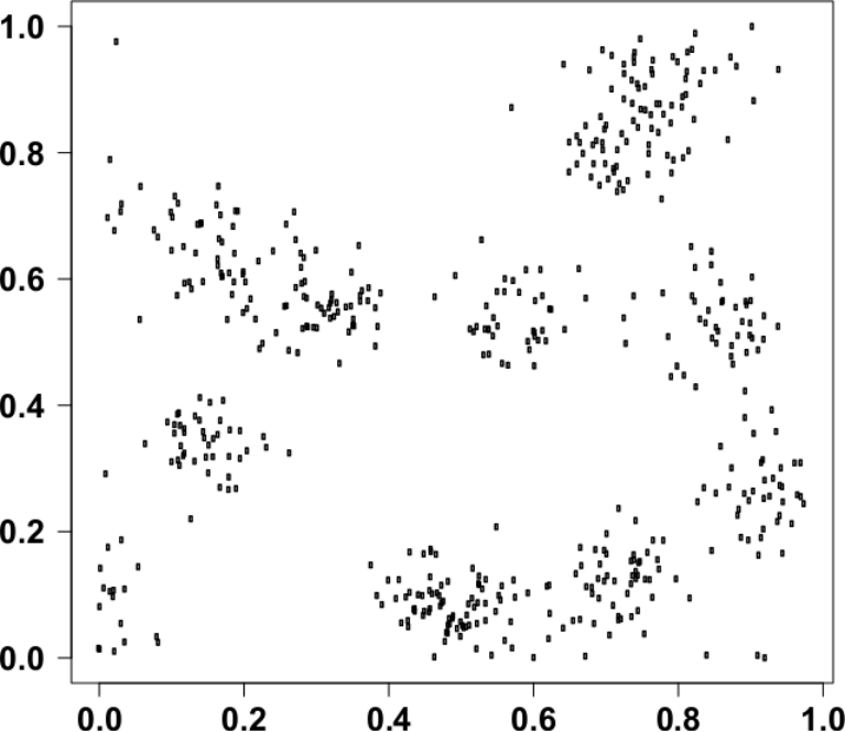
We first illustrate the influence of the estimation of the pair correlation function onto the accuracy of prediction on a single simulation. The simulated pattern, the associated theoretical intensity and the observation window, with a rate of of observed areas, are represented in Figures 6.a) to c) respectively.
a) b) c)
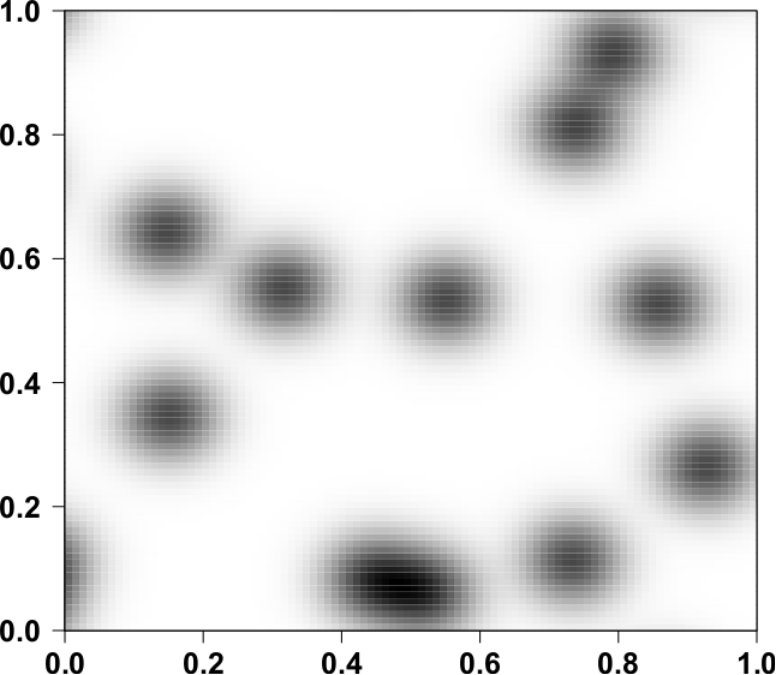

d) e) f)


The theoretical (dotted line) and estimated (solid line) pair correlation function are given in Figure 6.d). Figures 6.e) and f) illustrate the theoretical local intensity in and the prediction in on a grid, using the true (e) and the estimated (f) pair correlation function. In the first case, the prediction is relatively smooth and gives accurate results. In the second case, the prediction is more noisy, but recover the same blocks with high intensity values. In both cases, the method correctly predict the clusters when there are observations close to the unobserved bands. That is the case for all clusters located at the right hand side of the vertical line . When the full cluster falls in the unobserved band, as the ones located at the left hand side of the vertical line the method fails in predicting the cluster.
We plotted (Figure 7) the boxplot of the coefficient of determination resulting from 100 simple linear regressions between the predicted values of the local intensity and the theoretical ones, for different grid size (, and ), when the pair correlation function is estimated (Figure 7.b)) or not (Figure 7.a)). These results are related to an observation rate of 50%, according to the window configuration highlighted Figure 4. We obviously see that the goodness of prediction increases when the grid resolution increases and when the pair correlation function is known. We considered a grid as it is a trade off between computation times and a small mesh, allowing a good description of the intensity variations due to clusters. We obtained, in the worst case where the pair correlation function is estimated, that the coefficient of determination is around (median).
a) b)


6 Discussion
Our kriging method introduced to estimate and/or predict the local intensity of a stationary and isotropic point process has a large number of advantages, particularly in prediction. Taking into account the spatial structure of the point pattern allows to perform the intensity estimation for point processes highly aggregated at fine scale. In the prediction framework, our kriging method is innovative for the interpolation of the local intensity and presents good statistical properties (unbiasedness, low variance…) when the pair correlation function is known. When it is estimated, the quality of our interpolator is slightly reduced but our results can be improved by better taking into account the double estimation of the pair correlation function and the local intensity on the same pattern.
This prediction method is less time consuming than the reconstruction methods and appears a promising way in prediction of intensity of a spatial point pattern. Note that existing prediction methods are constrained within a class of point processes ([12], in particular Cox processes [10, 8, 11, 9]), making any comparison with our method very restrictive relatively to its broad scope of applications. That is for instance the case of any point process obtained by a weak dependent process (e.g. Thomas, Markov) with a parameter driven by a stationary random field at a larger scale (e.g. Cox), but not only.
Relaxing the stationary assumption implies to make further assumptions. The formalism should be quite similar to the one of this paper, but with some confounding effects as the ones observed when using the same point pattern to estimate both a spatially varying intensity and second-order characteristics [24, 25]. For instance, if we consider a non stationary Cox process, we cannot disentangle the first-order non-stationarity to the second-order non-stationarity. One could thus allocate the effects at different scales.
In our simulations and application, we used the R function solve, based on the LU factorization, to compute the inverse of the covariance matrix . This matrix is of dimension the square of the number of cells of the grid superimposed on the observation window. Thus, it can quickly become heavy to inverse. In such cases, estimating the matrix using Equation (8) would be somewhat cumbersome. Thus, we propose instead to inverse the covariance matrix numerically. Several approximations could be used, depending mainly on the width of with respect to and the curvature of the pair correlation function:
- 1.
if the diameter of is large, the covariance between two tiles at distance is equal to . It can be approximated numerically by computing for example the integral on a fine grid. Then the finer the grid, the smaller the difference between the exact values and the approximations, but the computing time cost can become prohibitive.
- 2.
when the diameter of becomes small, the integral can be approximated by so that the covariance is approximated by ,
- 3.
when the diameter becomes very small, may be approximated by , a situation seldom met in practice, since it needs a tile small enough to neglect point dependence.
Approximation 2) will thus be the most reasonable one, needing only a small enough to consider that is almost constant for , but avoiding too small leading to large matrix inversion time.
Our estimation is roughly pixellated compared to kernel methods, but it does not oversmooth the intensity of highly aggregated point processes. We could take the benefit of the two approaches to get smoother estimations. Our on-going work consists in regularizing the counting process by a kernel and in defining a kriging estimator for the related random field. Our optimal grid could then be used to define an optimal bandwidth, thus eliminating the Poisson aspect of classical kernels.
Our method provides good predictions in areas at small distances of data locations. From the definition of the kriging predictor, at distances larger than the range of interaction, it only provide a constant mean value. To improve it and make it more relevant in practice, we could consider further information provided by covariates. From our application point of view, wheat field mapping could be of interest as Montagu’s Harriers nest in there. From a methodological point of view, including covariates would imply that we should either consider external drift kriging (or any other universal kriging) rather than ordinary kriging); or spatial regression.
Finally, our kriging predictor depends on the count data in the grid cells, , and not on exact data locations in . Thus we can further consider count data sets, as it is often the case in biodiversity measures, e.g. plant species abundance. The exact position of each plant is rarely given, but we know its abundance per small unit areas. So, once the pair correlation function is estimated from the point data subset, one can apply our method to interpolate the intensity.
References
References
- [1] B. Silverman, Density Estimation for Statistics and Data Analysis, Chapman & Hall/CRC, London, 1986.
- [2] Y. Guan, On consistent nonparametric intensity estimation for inhomogeneous spatial point processes, Journal of the American Statistical Association 103 (483) (2008) 1238–1247.
- [3] M.-C. van Lieshout, Estimation of the intensity function of a point process, Methodology and Computing in Applied Probabilty 14 (2012) 567–578.
- [4] J. Illian, A. Penttinen, H. Stoyan, D. Stoyan, Statistical Analysis and Modelling of Spatial Point Patterns, John Wiley & Sons, London, 2008.
- [5] W. Härdle, Smoothing techniques, with implementation in S, Springer & Verlag, New York, 1991.
- [6] L. Devroye, The double kernel method in density estimation, Les Annales de l’I.H.P., section B 25 (4) (1989) 533–12.
- [7] A. Tscheschel, D. Stoyan, Statistical reconstruction of random point patterns, Computational Statistics and Data Analysis 51 (2006) 859–871.
- [8] P. Diggle, P. Ribeiro, Model-Based Geostatistics, Springer, New York, 2007.
- [9] P. Diggle, P. Moraga, B. Rowlingson, B. Taylor, Spatial and spatio-temporal log-gaussian cox processes: Extending the geostatistical paradigm, Statistical Science 28 (4) (2013) 542–563.
- [10] P. Monestiez, L. Dubroca, E. Bonnin, J. Durbec, C. Guinet, Geostatistical modelling of spatial distribution of balaenoptera physalus in the northwestern mediterranean sea from sparse count data and heterogeneous observation efforts, Ecological Modelling 193 (2006) 615–628.
- [11] E. Bellier, P. Monestiez, G. Certain, J. Chadœuf, V. Bretagnolle, Reducing the uncertainty of wildlife population abundance: model-based versus design-based estimates, Environmetrics 24 (7) (2013) 476–488.
- [12] M.-C. van Lieshout, A. Baddeley, Extrapolating and interpolating spatial patterns, in: In Spatial Cluster Modelling, A.B. Lawson and D.G.T. Denison (EDS.) Boca Raton: Chapman And Hall/CRC, Press, 2001, pp. 61–86.
- [13] G. Matheron, Traité de géostatistique appliquée: Mémoires du Bureau de Recherches Géologiques et Minières. Tome I, no. 14, Editions Technip, Paris, 1962.
- [14] G. Matheron, Traité de géostatistique appliquée: Le krigeage. Tome II, no. 24, Editions BRGM, Paris, 1963.
- [15] N. Cressie, Statistics for Spatial Data, revised Edition, John Wiley & Sons, New York, 1993.
- [16] H. Wackernagel, Multivariate Geostatistics: An Introduction with Applications, 3rd Edition, Springer-Verlag, 2003.
- [17] S. Chiu, D. Stoyan, W. Kendall, J. Mecke, Stochastic Geometry and Its Applications, 3rd Edition, John Wiley & Sons, New York, 2013.
- [18] J. Zhang, P. Atkinson, G. M.F, Scale in Spatial Information and Analysis, Taylor & Francis, 2014.
- [19] J. Chilès, P. Delfiner, Geostatistics: Modeling Spatial Uncertainty, 2nd Edition, John Wiley & Sons, New York, 2012.
- [20] K. Petersen, M. Pedersen, The Matrix Cookbook, Technical University of Denmark, 2012.
- [21] D. Stoyan, H. Stoyan, Fractals, random shapes and point fields: methods of geometrical statistics, John Wiley & Son, 1994.
- [22] P. Diggle, A kernel method for smoothing point process data, Applied Statistics 34 (1985) 138–147.
- [23] A. Baddeley, R. Turner, Spatstat: an R package for analyzing spatial point patterns, Journal of Statistical Software 12 (6) (2005) 1–42.
- [24] P. Diggle, V. Gómez-Rubio, P. Brown, A. Chetwynd, S. Gooding, Second-order analysis of inhomogeneous spatial point processes using case-control data, Biometrics 63 (2) (2007) 550–557.
- [25] E. Gabriel, Estimating second-order characteristics of inhomogeneous spatio-temporal point processes: influence of edge correction methods and intensity estimates, Methodololy and Computing in Applied Probability 16 (2) (2014) 411:431.
Appendix A Proof of Lemma 2.1
The following convergence result
ends the proof.
Appendix B Proof of Proposition 2.2
1)
2) follows from lemma 2.1 :
3) follows from the approximation
in lemma 2.1.4).
Appendix C Proof of Equations (12) and (13)
Let a square centered at of area . We denote by the gradient vector
By the following Taylor expansion around the origin
we obtain that:
and so
By consequence when estimating the local intensity, we have from Equation (10)
Deriving by the variable gives
and thus the solution of is
which is a minimum.
Appendix D Optimal mesh in practice
The optimal mesh of the estimation grid, , depends on the unknown terms and . In this section, we compare different methods which could be used to compute in practice. We simulated point patterns in the unit square from Thomas point processes with different set of parameters: and . Then, is computed as follows. First we estimate/compute the intensity on a grid. Second, we deduce its gradient from the rate of change between the estimated intensity and its one-cell translated value. Third, we compute and its related grid size (in number of pixels).
We used different methods to estimate the intensity. The counting method consists in estimating the local intensity in each pixel by . The global kernel smoothing method is based on a gaussian kernel estimator with global bandwidth and without border correction, so , where is the density function of a standard normal distribution. The -nearest neighbours method is an adaptive nonparametric estimation so that , with the distance of to its -nearest neighbour. Note that we also compute the theoretical value of the intensity from Equation (14).
We considered three -grids, with . We compared the distributions of the optimal grid sizes obtained from 100 realisations of each process and from the different methods, to the theoretical ones. We select the method which provides the more accurate results and the less sensitivity to the different scenarii.
If the counting method works well when the pattern is strongly aggregated at very small scale (), it requires a fine grid and is inaccurate for other scales of clustering. Thus in the following it will be no longer considered. The other methods provide globally much better values of the optimal grid size. While may be roughly estimated, the integral of its gradient is sufficiently well approximated to obtain good results. Figure 8 shows the optimal grid sizes (in number of pixels) obtained from different size of the estimation grid: (solid line), (dashed line) and (dotted line).
The theoretical grid size is in black and the ones derived from the kernel smoothing and the -nearest neighbours method are in red and green respectively. This figure is related to the Thomas process with parameters , , and we get similar results from the other set of parameters. It appears that the -nearest neighbours based method is very sensitive to the size of the estimation grid and tends to over-estimate the optimal grid size. The kernel based method under-estimates the optimal grid size when the estimation grid is not fine enough and when the scale of clustering in very small.
From this simulation study, we recommend the kernel based method on a grid to first estimate and then compute the optimal mesh or equivalently the optimal grid size.