Prasanna Kumar. K IIT Bombay, Mumbai 400076, India prasannak@cse.iitb.ac.in \authorinfoAmitabha Sanyal IIT Bombay, Mumbai 400076, India as@cse.iitb.ac.in \authorinfoAmey Karkare IIT Kanpur, Kanpur 208016, India karkare@cse.iitk.ac.in
Liveness-Based Garbage Collection for Lazy Languages
Abstract
We consider the problem of reducing the memory required to run lazy first-order functional programs. Our approach is to analyze programs for liveness of heap-allocated data. The result of the analysis is used to preserve only live data—a subset of reachable data—during garbage collection. The result is an increase in the garbage reclaimed and a reduction in the peak memory requirement of programs. While this technique has already been shown to yield benefits for eager first-order languages, the lack of a statically determinable execution order and the presence of closures pose new challenges for lazy languages. These require changes both in the liveness analysis itself and in the design of the garbage collector.
To show the effectiveness of our method, we implemented a copying collector that uses the results of the liveness analysis to preserve live objects, both evaluated and closures. Our experiments confirm that for programs running with a liveness-based garbage collector, there is a significant decrease in peak memory requirements. In addition, a sizable reduction in the number of collections ensures that in spite of using a more complex garbage collector, the execution times of programs running with liveness and reachability-based collectors remain comparable.
Keywords:
Algorithms, Languages, Theorycategory
D.3.4 Programming Languages Processorskeywords
Memory Management (Garbage Collection), Optimizationscategory
F.3.2 Logic and Meanings Of Programs Semantics of Programming Languageskeywords
Program Analysiskeywords
Heap Analysis, Liveness Analysis, Memory Management, Garbage Collection, Lazy Languages1 Introduction
Functional programs make extensive use of dynamically allocated memory. The allocation is either explicit (i. e., using constructors) or implicit (creating closures). Programs in lazy functional languages put additional demands on memory, as they require closures to be carried from the point of creation to the point of evaluation.
While the runtime system of most functional languages includes a garbage collector to efficiently reclaim memory, empirical studies on Scheme [19] and on Haskell [26] programs have shown that garbage collectors leave uncollected a large number of memory objects that are reachable but not live (here live means the object can potentially be used by the program at a later stage). This results in unnecessary memory retention.
In this paper, we propose the use of liveness analysis of heap cells for garbage collection (GC) in a lazy first-order functional language. The central notion in our analysis is a generalization of liveness called demand—the pattern of future uses of the value of an expression. The analysis has two parts. We first calculate a context-sensitive summary of each function as a demand transformer that transforms a symbolic demand on its body to demands on its arguments. This summary is used to step through function calls during analysis. The concrete demand on a function body is obtained through a conservative approximation similar to 0-CFA [31] that combines the demands on all the calls to the function. The result of the analysis is an annotation of certain program points with deterministic finite-state automata (DFA) capturing the liveness of variables at these points. Depending on where GC is triggered, the collector consults a set of automata to restrict reachability during marking. This results in an increase in the garbage reclaimed and consequently in fewer collections.
While the idea of using static analysis to improve memory utilization has been shown to be effective for eager languages [6, 15, 16, 21], a straightforward extension of the technique is not possible for lazy languages, where heap-allocated objects may include closures (runtime representations of unevaluated expressions). Firstly, since data is made live by evaluation of closures, and in lazy languages the place in the program where this evaluation takes place cannot be statically determined, laziness complicates liveness analysis itself. Moreover, for liveness-based GC to be effective, we need to extend it to closures apart from evaluated data. Since a closure can escape the scope in which it was created, it has to carry the liveness information of its free variables. As execution progresses and possible future uses are eliminated, we update the liveness information in a closure with a more precise version. For these reasons, the garbage collector also becomes significantly more complicated than a liveness-based collector for an eager language.
Experiments with a single generation copying collector (Section 6) confirm the expected performance benefits. Liveness-based collection results in an increase in garbage reclaimed. As a consequence, there is a reduction in the number of collections from 1.6X to 23X and a decrease in the minimum memory requirement from 1X to 1389X. As an added benefit, there is also a reduction in the overall execution time in 5 out of 12 benchmark programs.
1.1 Motivating example
Figure 1 shows an example program and the state of the heap at the program point 11 1 We write to associate a label with the program point just before the expression . The label is not part of the syntax., i.e., just before the evaluation of . The heap is represented by a graph in which a node either represents atomic values (, integers, etc.), or a cell containing and fields, or a closure (represented by shaded clouds). Edges in the graph are references and represent values of variables or fields. The figure shows the lists x and z partially evaluated due to the condition ( ( z)). The edges shown by thick arrows are those which are live at . Thus if a GC takes place at with the heap shown in Figure 1(b), a liveness-based collector (LGC) will preserve only the cells referenced by z, and the live cells constituting the closure referenced by . In contrast, a reachability-based collector (RGC) will preserve all cells.
In this work we show that static analysis of heap data can help garbage collectors in reclaiming more garbage. The specific contributions of this paper are:
- •
We propose an interprocedural liveness based GC scheme for a lazy first-order functional language and prove its correctness. To the best of our knowledge, this is the first work that uses the results of an interprocedural liveness analysis to garbage collect both evaluated data and closures. Thomas [32] describes a copying garbage collector for the Three Instruction Machine (TIM) [11] that only preserves live closures in a function’s environment (also called a frame). However, in the absence of details, it is not clear whether a) the scope of the method is interprocedural, and b) it handles algebraic datatypes like lists (the original design of TIM did not). All other previous attempts [27, 29, 28, 6, 19] involved either imperative or eager functional languages.
- •
We formulate a liveness analysis for the lazy first-order functional language and prove its correctness. The proof involves specifying liveness for the language through a non-standard semantics and then proving the analysis correct with respect to the specification.
- •
The analysis results in a set of context-free grammars along with a fixed set of non-context-free productions. The decision whether to copy a cell during GC translates to a membership problem for such grammars. Earlier research assumed the undecidability of this membership question and used an over-approximation to overcome it. In this paper, we provide a formal proof of the undecidability of this problem.
- •
We have implemented a garbage collector that uses the result of liveness analysis to retain live cells. Our experiments reveal interesting space-time trade-offs in the engineering of the collector—for example, updating liveness information carried in closures during execution results in more garbage being collected. Empirical results show the effectiveness of liveness-based GC.
1.2 Organization of the paper
Section 2 introduces the syntax of the programming language considered and gives a small-step operational semantics for it. The liveness analysis for this language and its soundness proof is presented in Section 3. Section 4 describes the formulation of liveness as grammars. We also give a proof of undecidability of such grammars and show how they can be approximated by DFAs. Section 5 discusses details of the garbage collector, in particular the use of liveness DFAs for GC. We report our experimental results in Section 6 along with some observations. Section 7 discusses previous work related to GC and liveness and Section 8 discusses possible extensions and concludes the paper.
2 The target language—syntax and semantics
Figure 2 describes the syntax of our language. It is a first order language with lazy semantics. Programs are restricted to be in Administrative Normal Form (ANF) [8], where all actual parameters to functions are variables. While this restriction does not affect expressibility, this form has the benefit of making explicit the creation of closures through the construct. We assume that s in our language are non-recursive; in the expression , should not occur in . The restriction of to a single definition is for ease of exposition—generalization to multiple definitions does not add conceptual difficulties. We further restrict each variable in a program to be distinct, so that no scope shadowing occurs; this simplifies reasoning.
We denote the body of a function as . We assume that each program has a distinguished function , defined as, and the program begins execution with the call to .
| Premise | Transition | Rule name |
| const | ||
| cons | ||
| car-select | ||
| car-1-clo | ||
| car-clo | ||
| prim-add | ||
| prim-1-clo | ||
| prim-2-clo | ||
| funcall | ||
| is a new location | let | |
| if-true | ||
| if-false | ||
| if-clo | ||
| return-whnf | ||
| return-clo |
2.1 Semantics
We now give a small-step semantics for our language. We first specify the domains used by the semantics:
Here is a countable set of locations in the heap. A non-empty location either contains a closure, or a value in Weak Head Normal Form (WHNF)[25]. In our case, a WHNF value can be a number, the empty list or a cell with possibly unevaluated constituents. A closure is a pair in which is an unevaluated application, and maps free variables of to their respective locations. Since all data objects are boxed, we model an environment as a mapping from the set of variables of the program to locations in the heap.
The semantics of expressions (and applications22 2 In most contexts, we shall use the term ’expression’ and the notation to stand for both expressions and applications.) are given by transitions of the form . Here is a stack of continuation frames. Each continuation frame is a triple , signifying that the location has to be updated with the value of the currently evaluating expression and is to be evaluated next in the environment . The initial state of the transition system is:
in which , and are are the empty environment, heap and stack respectively. The initial stack consists of a single continuation frame in which ans is a distinguished variable that will eventually be updated with the value of (), and maps ans to a location . In addition, is a function modeling a printing mechanism—a standard run-time support assumption for lazy languages [25]—that prints the value of (). The operator pushes elements on top of the stack.
The notation represents an environment that maps variables to locations and indicates updation of at with . represents the environment shadowed by and represents the environment restricted to the variables in . Finally represents the free variables in the application and gives the address of the closure in the heap.
The small-step semantics is shown in Figure 3. Unlike an eager language, evaluation of a let expression does not result in the evaluation of . Instead, as the let rule shows, a closure is created and bound to . The program points which trigger evaluation of these closures are an condition (IF-clo) and a (return-clo). We call such points evaluation points and label them with instead of . As an example of closure evaluation, we explain the three rules for . If is a closure, it is evaluated to WHNF, say . This is given by the rule car-clo. If is not in WHNF, it is also evaluated (car-1-clo). The address to be updated with the evaluated value is recorded in a continuation frame. This is required for the evaluation to be lazy, else may be evaluated more than once due to sharing [25]. Only after this is the actual selection done (car-select).
3 Liveness
A variable is live if there is a possibility of its value being used in future computations and dead if it is definitely not used. Heap-allocated data needs a richer model than classical liveness—a model which talks about liveness of references.
An access path is a prefix-closed set of strings over , where , represent access using and fields respectively. Given an initial location (usually a reference corresponding to a variable) and a heap , semantically an access path represents a reference, denoted , in the heap that is obtained by starting with and chasing the or fields in the heap as specified by the access path. is defined only if the path followed in the heap is closure-free (does not cross closures), else it is undefined.
Access paths are used to represent liveness. As an example, a list with liveness means that future computations only refer up to the second and third members of . A liveness environment is a mapping from variables to access paths, but often expressed as a set, for example by writing instead of . In this notation, represents access using itself and indicates is dead. In lazy languages, liveness environments are associated with regions of programs instead of program points.
A notion that generalizes liveness is demand. While liveness gives the patterns of future uses of a variable, demand represents the future uses of the value of an expression. The demand on an expression is also a set of access paths—the subset of which the context of may explore of ’s result. To see the need for demands, consider the expression . Assume that the context of this expression places the demand . Since the value of the expression is the value of , the demand translates to the liveness . Due to the definition which binds to , the liveness of now becomes the demand on . This, in turn, generates the liveness . These are the -rooted accesses required to explore paths of the result of .
We use to range over demands, to range over access paths and to range over liveness environments. The liveness of an individual variable in is , but more commonly written as . The notation denotes the set . Often we shall abuse notation to juxtapose an edge label and a set of access paths; is a shorthand for .
| ( (f x) |
| :( y ( x) |
| ( :y |
| ( u ( x) |
| ( w (/ u y) ( :w))) |
| ( z (+ y 1) ( :z))))) |
(live-define)
3.1 Liveness analysis for lazy languages
Consider the program in Figure 4. As mentioned earlier, a lazy evaluation of the expression at creates a closure for instead of evaluating it. Since the closure may escape the scope in which it is created, it carries a copy of x within itself. We treat the copy of x in the closure as being separate from the x introduced by the , and call it a closure variable. For liveness calculations, such variables are distinguished from variables introduced by s and function arguments (called stack variables, since they reside in the activation stack). We notationally distinguish a closure variable from its corresponding stack variable by subscripting it with the label of the program point where the closure was created33 3 Multiple occurrences of the same variable in an application are further distinguished by their positions in the application..
Since a closure is evaluated only at evaluation points, a closure variable is attributed with the same liveness in the entire region of the program from the point of creation of the closure to reachable evaluation points. This is also true of stack variables, because, as we shall see, stack variables derive their liveness from closure variables. Thus, there are two major differences between our formulation of liveness of lazy languages with liveness of eager languages [6]: (i) the introduction of closure variables in the liveness calculations, and (ii) a single liveness value for each variable that is applicable from its creation point to evaluation points.
Closure variables get their liveness values through a chain of dependences beginning at a variable at an evaluation point. As an example, in Figure 4, a dependence chain for begins with the variable z at the evaluation point . The variable z returned at depends on y through the expression . y in turn depends on the closure variable through . We denote this chain of dependences as . Indeed, the chains of closures in the heap are a runtime representation of these dependences. Since z is evaluated at due to the expression z, the demand made by the calling context(s) of places a demand on z which will impart a liveness to . Other dependence chains which result in a liveness for are and . The liveness analysis described in this section declares the liveness of to be a union of the liveness arising from these dependence chains. To be safe, a GC during evaluation of y at has to use this liveness to copy the heap starting from . However, notice that if a GC takes place while evaluating z at , it can safely consider only the liveness arising from the dependence chain. The garbage collection scheme described in Section 5 uses a generalization of this observation to dynamically select an evaluation point specific liveness in order to collect more garbage.
Figure 5 describes our analysis which has two parts. The function , takes an application and a demand and returns the incremental liveness generated for the free variables of due to the application. This will be consulted during GC while exploring the heap starting from the closure variables. The function uses to propagate liveness across expressions.
In a lazy language, an expression is not evaluated unless required. Therefore the null demand () does not generate liveness in any of the rules defining or . A non-null demand of on ( ), is transformed to the liveness . In an opposite sense, the demand of on ( ) is transformed to the demand on . Since does not dereference its arguments, there is no demand on and . The rules for ( x y) and ( x) are similar. Constants do not generate any liveness.
In case of a function call, we use the third parameter that represents the summaries of all functions in the program. (the summary for a specific function ) expresses how the demand on a call to is transformed into the liveness of its parameters at the beginning of the call. is determined by the judgement using inference rule (live-define). This rule describes the fixed-point property to be satisfied by , namely, the demand transformation assumed for each function in the program should be the same as the demand transformation calculated from its body. As we shall see in Section 4, we convert the rule into a grammar and the language generated by this grammar is the least solution satisfying the rule. We prefer the least solution since it ensures the safe collection of the greatest amount of garbage.
We next describe the function that propagates liveness across expressions. Consider the -rules for , , and . Since the value of is the value of , a demand on gives a liveness of . The liveness of the expression is a union of the liveness of and . In addition, since the condition is also evaluated, the liveness is created and added to the union. To understand the liveness rule for , observe that the value of is the value of its body . Thus the liveness environment of is calculated for the given demand . Since the stack variable is copied to each of the closure variable , the liveness of is the union of the liveness of the closure variables. This liveness, say , is also the demand on , thus the liveness environment is added to . Finally, the stack variables corresponding to the free variables of are updated and added to give the overall liveness environment for .
As noted earlier, specifies the liveness of the reference only if corresponds to a closure-free path in starting from . If this path is intercepted by a closure, say , then the liveness of the path starting from is given by . As we shall see in Section 5, the liveness of the closure variable is recorded along with the closure for so that the GC can refer to it during garbage collection.
3.2 Soundness of analysis
We shall now present a proof of soundness of the analysis presented in Section 3.1. It is easy to see that the analysis correctly identifies the liveness of stack variables. A stack variable is live between its introduction through a and its last use to create a closure variable. This is correctly captured by the rule in Figure 5. Proving soundness for closure variables is more complex. Here are the ideas behind the proof.
- 1.
We augment the standard semantics in Figure 3 to model a GC before the execution of each expression. Note that, unlike eager languages, memory is allocated only during execution of expressions. During GC, we track each reference in the root set and heap that is declared dead by our analysis. Any attempt to dereference such references results in the transition system entering a special state denoted bang. We call the semantics after augmentation, minefield semantics.
- 2.
Assuming that a program enters the bang state, we construct, through inline expansion, a program without function calls which has the same minefield behavior. The final step shows that no program without function calls can enter the bang state. As a consequence no program (with or without function calls) can enter the bang state.
| Premise | Transition | Rule name |
| car-bang | ||
| car-1-clo | ||
| car-clo | ||
| , is a new location | where | let |
To set up the minefield semantics, we follow these steps:
- 1.
We extend the abstract machine state to . We call such a state a minefield state. Here is the “dynamic” demand on the expression , that arises from the actual sequence of function calls that led to the evaluation of .44 4 The static liveness that is consulted during actual GC is computed from an over-approximation of this demand. Thus the soundness result on the modeled GC will also apply for the actual GC. The demand for the initial state is , and each transition transforms the demand according to the liveness rules of Section 3.1. The information in continuation frames on the stack are also similarly augmented with their demands. Thus a stacked entry now takes the form .
- 2.
The closure created by a let expression is now a 3-tuple , where represents the demand on the closure.
- 3.
models a liveness-based garbage collection that returns . The changes in and are due to non-live references being replaced by . This simulates the act of garbage collecting the cells pointed to by these references during an actual garbage collection. To do so, needs to consider the following environments: (1) the environment in the current state, (2) the environment in each of the stacked continuations and (3) the environment in each of the closures in the heap.
- (a)
For each of these environments, calculates a liveness environment using the corresponding (or ) and .
- (b)
For each location , sets to iff for each environment above, for each , and each forward access path , it is not the case that and .
- (a)
Figure 6 shows some of the minefield rules. As mentioned earlier, the transition for a is preceded by . The details of the transition for the car-clo rule is also shown. If an earlier call to results in being bound to , then the step enters the bang state (car-bang). Otherwise the transition is similar to the earlier car-clo rule. The remaining rules for minefield semantics are given in Appendix A.
Consider a trace of a minefield execution of a program , possibly ending in a bang state. We can construct a call-tree based on the trace in which each node represents a function that was called (but did not necessarily return because of a bang). Assume that each of the nodes of the tree is also annotated with the program point where the corresponding call was invoked. This tree can be used to inline function calls in a hierarchical fashion. The details of the inlining can be found in [6]. For a call-less program, the initial state of the minefield semantics is assumed to be .
3.3 Soundness result
We first need an auxiliary result about minefield semantics. Consider a trace of a minefield execution. For every minefield state that appears on the LHS of a step, the demand on the expression (or application ) is non-null. This can be proved by an induction on the number of steps leading to the minefield state. The base step holds because the demand on is non-null. For the inductive step we observe that for each step of the minefield semantics, if the demand on the LHS of a minefield step is non-null, the demand on the RHS is a transformation of (for example ) which is also non-null.
Note that our proofs will be for a single round of minefield execution i.e., the evaluation of to its WHNF driven by the printing mechanism (Section 2.1). With minor variations, the proof will also be applicable for subsequent evaluations initiated by .
Lemma 3.1
Consider the minefield execution of a program without function calls. Such a program cannot enter the bang state.
Proof 3.2.
Consider a state in the minefield execution of a program. We show by induction on the number of steps leading to this state that the next transition cannot enter a bang state. When is 0, the state is . Since the call to in this state does nothing, we just have to show that the transition cannot enter a bang state. Since our programs are in ANF, can only be a expression. A let step does not involve dereferencing, and thus cannot result in a bang.
For the inductive step, we shall show that none of the minefield steps that involves dereferencing results in a bang. These are the steps which have a in the premise. Now a step can go bang because it dereferences a inserted by an earlier . However the demand on basis of which the would have inserted a would have included the current demand . Thus it is enough to show that the step would not lead to a bang, even if had been done with the current demand .
We consider the rules for only. The rest of the rules involve similar reasoning. For the car-clo rule in the state , we know that is non-null. Therefore the liveness of includes , and the dereferencing will go without bang.
For the car-1-clo rule, observe that there are two dereferences. First is dereferenced to get a cons cell and then the head of the cons cell is dereferenced to obtain a closure. If the demand on is non-null, then the liveness of will include both and , and a GC with this liveness will neither bind to a , nor insert at the first component of the cons cell. Thus both dereferences can take place without entering the bang state.
Now we are ready to prove the main soundness result.
Theorem 3.3.
The minefield execution of no program can enter a bang state.
Proof 3.4.
Assume to the contrary that a program enters the bang state. We can transform to a call-less program such that the minefield executions of and are identical except for change of variable names. However, by Lemma 3.1 we know that , a call-less program, cannot enter the bang state. Therefore also cannot enter the bang state.
4 Towards a computable form of liveness
The analysis in Section 3 is fully context-sensitive, describing the liveness sets in a function body in terms of a symbolic demand and . However, we have yet to describe (i) how to obtain demand transformers from the rule live-define , and (ii) how to compute the concrete demand on each function. To do so, we first need to modify the liveness rules to a slightly different form.
Symbolic representation of operations:
The rule for , shown in Figure 5, requires us to remove the leading and from the access paths in . Similarly, the rules for , , , , and require us to return , if itself is and otherwise. To realize these rules needs to be known. This creates difficulties since we want to solve the equations arising from liveness symbolically.
The solution is to also treat the operations mentioned above symbolically. We introduce three new symbols: , , . These symbols are defined as a relation between sets of access paths:
Thus selects those entries in that have leading , and removes the leading from them. The symbol reduces the set of strings following it to a set containing only . It filters out, however, the empty set of strings.
We can now rewrite the and the rules of as:
and the rule for as:
The rules for , and are also modified similarly.
When there are multiple occurrences of , and , is applied from right to left. The reflexive transitive closure of will be denoted as . The following proposition relates the original and the modified liveness rules.
Proposition 4.1.
Assume that a liveness computation based on the original set of rules gives the liveness of the variable as (symbolically, ). Further, let when the modified rules are used instead of . Then .
An explanation of why the proposition holds for the modified rule is given in [6]. The proposition also holds for other modified rules for similar reasons.
| ( ( l) |
| ( x ( l) |
| ( x |
| ( v |
| ( u ( l) |
| ( y ( u) |
| ( z (+ 1 y) ))))))) |
| ( a BIG closure ) |
| + |
| ( c |
| ( w |
Computing function summaries :
Given a function , we now describe how to generate equations for the demand transformation f. The program in Figure 7 serves as a running example. Starting with a symbolic demand , we determine . In particular, we consider , the liveness of the parameter . By the rule live-define, this should be the same as . Applying this to , we have:
In general, the equations for are recursive as in the case of f. A closed form solution for can be derived by observing that each of the liveness rules modifies a demand only by prefixing it with symbols in the alphabet . Therefore we can assume that has the closed form:
| (3) |
where are sets of strings over the alphabet mentioned above. Substituting the guessed form in the equation describing f, and factoring out , we get an equation for that is independent of . Any solution for yields a solution for f. Applied to length, we get:
Note that this equation can also be viewed as a CFG with {, } as terminal symbols and as the sole non-terminal.
Handling user-defined functions:
To avoid analyzing the body of a function for each call, we calculated the liveness for the arguments and the variables in a function with respect to a symbolic demand . To get the actual liveness we calculate an over-approximation of the actual demands made by all the calls and calculate the liveness at each GC point inside the function based on this approximation. The 0-CFA-style summary demand is calculated by taking a union of the demands at every call site of a function.
For the running example (Figure 7), has calls from at and a recursive call at . The demands on these calls are and . Thus:
As examples, the closure variables and , and the stack variables l and a have the following liveness in terms of :
In summary, the equations generated during the analysis are:
- 1.
For each function , equations defining for use by f.
- 2.
For each function , an equation defining the summary demand on .
- 3.
For each function (including ) an equation defining liveness for each garbage in .
From liveness sets to context-free grammars:
The equations above can now be re-interpreted as a context-free grammar (CFG) on the alphabet . Let X denote the non-terminal for a variable occurring on the LHS of the equations generated from the analysis. We can think of the resulting productions as being associated with several grammars, one for each non-terminal regarded as a start symbol. As an example, the grammar for and comprise the following productions:
Other equations can be converted similarly. The language generated by , denoted , is the desired solution of . However, recall that the decision problem that we are interested in during GC is: Let be a forward access path (consisting only of edges and but not , or ). Let , where consists of forward access paths only. Then does ? We model this problem as one of deciding the membership of a CFG augmented with a fixed set of unrestricted productions.
Definition 4.2.
Consider the grammar in which is a set of non-terminals, , is a set of context-free productions that contains the distinguished production , is a string of grammar symbols that does not contain , and is the fixed set of unrestricted productions , , , , and .
We first show that membership problem of the class of grammars in Definition 4.2 is undecidable. However note that the grammars may not be necessarily generated from liveness analysis.
Lemma 4.3.
Given a grammar of the kind described in Definition 4.2 and a forward access path consisting of symbols and only, the membership problem is undecidable.
Proof 4.4.
Given a Turing machine and an input , we construct a grammar such that the machine will halt on if and only if . The grammar includes the fixed set of unrestricted productions in Definition 4.2.
We shall represent a Turing machine (TM) configuration as , where is the string to the left of the head, is the string to the right, is the symbol under the head and is the current state of the TM. For each combination of state and symbol , the grammar will contain the non-terminal . We shall synchronize each move of the TM to a derivation step using a context free production, followed, if possible, by a derivation step using either or . After each synchronization, we shall establish the following invariant relation between the TM configuration and the sentential form:
If the configuration of the TM is , then the sentential form will be , where is the same as but with each symbol in replaced by .
Assume that the TM starts in a state with a tape and the head positioned on the symbol . Then the sentential form corresponding to the initial configuration is (we can assume that there is a production , where is the start symbol of the grammar). Further correspondences between the TM moves and the grammar productions are as follows:
- 1.
For each transition , there are two productions and .
- 2.
For each transition , there are two productions and .
The idea behind the productions is explained with an example: Assume that the current sentential form is . Also assume that the TM has a transition . Since the next corresponding step in the derivation has to be done without any prior knowledge of whether the symbol to the left of the tape is a or a , two productions are provided, and the invariant will be maintained only if the production is chosen for the next step in the derivation. This gives the configuration . Simplification with the production yields , which exactly corresponds to the changed configuration of the TM. Notice carefully that a wrong choice breaks the invariant and it cannot be recovered subsequently by any choice of productions.
After the TM has halted, there are further “cleanup” derivations that derive only if the invariant has been maintained so far. For every symbol , we introduce a non-terminal where is the final state of the TM. We add productions and for cleaning up the and symbols on the left of the head and and for cleaning up and on the right of the tape head. This completes the reduction.
We now show that the proof can be replayed for the class of grammars generated from liveness analysis of programs.
Lemma 4.5.
Given a grammar of the kind described in Definition 4.2 that is generated by liveness analysis of a program and a forward access path , the membership problem is undecidable.
Proof 4.6.
Given a Turing machine and an input string, the proof of Lemma 4.3 generates a grammar. We shall define a function for each non-terminal introduced in this grammar such that the liveness analysis of the function will result in a set of productions that includes the productions for generated for the proof. As an example, it can be verified that the grammar for the function shown in Figure 8(b) includes the productions shown in Figure 8(a). Here corresponds to the demand .
The body of the function corresponds to the RHS of the productions for . Productions with the same LHS non-terminal, but with differing non-terminal on RHS can be generated by joining program fragments with . If there are such functions, then creates a -way branch and inserts a single call to a distinct function in each branch.
| ( ( a) |
| ( b ( a) |
| ( c ( b) |
| ( d ) |
| ( e ( c d)) |
| ( e)))))) |
(a) (b)
Notice that each production in Lemma 4.3 had a single non-terminal on the RHS. There are two characteristics of the grammar produced from liveness-analysis that are are relevant for replaying the earlier proof: (a) If was a production in the earlier proof, the grammar generated from liveness analysis of the constructed program will have the production , and (b) other productions are of the form .
It is clear that if the TM given as an instance of the halting problem accepts the input string, then the earlier derivation can be replayed, every time replacing in the sentential form by . However, if the TM does not accept the input string, then every sentential form derived from the start symbol would have at least one non-terminal from the grammar of Lemma 4.3 that is different from . Thus would not be derivable from the grammar.
We circumvent the problem of undecidability by over approximating the CFG by non-deterministic finite state automata (NFA) using Mohri and Nederhof [23] method. For example, the grammar fragment for after the Mohri-Nederhof transformation is:
The strongly regular grammar is converted into a set of NFAs, one for each . The simplification is now done on the NFAs by repeatedly introducing edges to bypass pairs of consecutive edges labeled or and constructing the -closure till a fixed point is reached, after which the edges labeled and are deleted. The resulting automaton has edges labeled with , and only. In this automaton, for every edge labeled , we check if the source node of the edge has a path to a final state. If it does, we mark the source node as final. Finally, we remove all the edges labeled and convert the automaton into a deterministic automaton. These steps effectively implement the simplification rules for , , and to obtain forward access paths. While checking for liveness during garbage collection, a forward access path is valid only if it can reach a final state. Figure 9(a) shows the NFA that is obtained from the grammar for , and the final DFA is shown in Figure 9(b). This expectedly says that for a demand , the liveness of the argument of is (the spine of the list is traversed). Similarly, Figure 9(c) shows the NFA for . The DFA in Figure 9(d) does not accept any forward paths, reflecting the lazy nature of our language. Since does not evaluate the elements of the argument list, the closure for a is never evaluated and is reclaimed whenever liveness-based GC triggers beyond .
5 The GC scheme
In the liveness analysis described in Section 3.1, the liveness of a closure variable is derived from dependence chains along all paths from the program point where the closure was created to reachable evaluation points. Assume, for the sake of concreteness, that and are two such evaluation points. During GC, we would like to use a more precise liveness, based on the actual paths taken during execution. Therefore we create separate liveness automata for dependences along paths to and , in addition to automata for dependences along paths to both and . The closure carries the liveness environment for its free variables (as pointers to automata, one for each variable). Initially the liveness environment is based on the dependences along both and . However, after evaluating an condition, the liveness environments are updated to one based on either or , so that subsequent garbage collections are based on more precise liveness information.
Based on the above considerations, we restrict the possible garbage collection points in a function body to the following:
- 1.
We statically over-approximate the memory required to create the closures for each function body. On entering a function, if the available memory is less than this requirement for the function, a GC is triggered.
- 2.
Since the evaluation of a condition may trigger a collection, after evaluating the condition the available memory is checked once again against a revised estimate of the memory (based on value of the condition) required to execute the rest of the program. A GC is triggered if enough memory is unavailable.
We shall call a unit of allocatable memory as a cell. A cell can hold a basic value (), the constructor ) or a closure. The closure, in turn, can be one of (), () and function application (. Here each is a reference to another heap cell. In addition, the closure also carries a pointer to a DFA (denoted ) for each . Algorithm 1 describes the garbage collection scheme. Starting with the root set, each cell pointed by a live reference (i.e., whose associated DFA state is final) is copied using . Copying a cells just involves copying the cell itself and conditionally copying the and the fields after referring to the next states of the DFA. If the reference points to a closure, then, as noted earlier, the closure carries pointers to the liveness DFAs of its arguments. These are used to recursively initiate copying of the arguments. Note that the copying strategy for or are similar to and have not been shown.
| Program |
fibheap |
sudoku |
nperm |
paraffins |
lcss |
huffman |
knightstour |
nqueens |
deriv |
treejoin |
lambda |
gc_bench |
| #CFG Nonterminals | 621 | 1422 | 662 | 1174 | 642 | 499 | 660 | 404 | 328 | 615 | 669 | 390 |
| #CFG Rules | 1176 | 2009 | 866 | 1773 | 1206 | 818 | 883 | 643 | 468 | 1328 | 1088 | 450 |
| #DFA States | 1761 | 4283 | 1546 | 3346 | 1666 | 1414 | 1519 | 889 | 809 | 1803 | 1703 | 571 |
| #DFA Transitions | 2829 | 7690 | 2522 | 6086 | 2726 | 2528 | 2420 | 1170 | 1435 | 2797 | 2580 | 788 |
| DFA Gen Time (sec) | 37.28 | 655.41 | 0.94 | 13.22 | 8.66 | 4.00 | 10.97 | 0.36 | 0.61 | 903.14 | 11.01 | 0.10 |
(a) Data for Liveness Analysis
#Cells collected/GC
#Cells touched/GC
#GCs
Peak Memory Required
GC time (sec)
Total Exec time (sec)
Program
RGC
LGC
RGC
LGC
RGC
LGC
RGC
LGC
RGC
LGC
RGC
LGC
fibheap
3466.2
4164.5
33576.6
50957.9
1333
1108
37043
37043
1.16
1.46
20.00
13.70
13.82
33.23
2.40
sudoku
931.3
2328.7
3134.6
2950.2
179
72
4066
2960
0.84
0.01
0.04
4.64
0.11
0.16
1.5
nperm
4684.4
14212.5
22743.2
23127.1
710
235
27428
25343
1.07
0.24
1.24
5.20
1.80
3.39
1.88
paraffins
661.7
2920.5
4522.6
2933.0
16
4
5185
3733
0.83
0.00
0.00
2.01
0.01
0.02
1.2
lcss
8064.7
18268.7
14177.9
4604.4
30
14
22243
16296
0.84
0.01
0.02
3.02
0.13
0.18
1.36
huffman
10533.8
100010.0
89536.1
88.6
356
38
100070
72
0.00
0.64
0.01
0.02
2.70
2.55
0.94
knightstour
179155.0
312454.0
498645.0
534562.0
529
304
677800
642303
1.09
6.24
64.43
10.32
55.29
134.35
2.43
nqueens
2607.4
9529.1
7493.4
829.0
3345
916
10101
1082
0.12
0.36
0.18
0.49
4.68
5.87
1.25
deriv
854.6
10755.3
10269.3
420.3
31
3
11124
589
0.06
0.00
0.00
0.05
0.05
0.05
0.9
treejoin
50284.2
936525.0
1566250.0
700756.0
116
5
1616533
887005
0.63
3.84
1.90
0.49
6.66
5.50
0.82
lambda
7271.7
8448.4
13194.2
29156.3
775
667
20466
18169
1.02
0.17
4.70
28.48
2.77
8.32
3.00
gc_bench
14932.7
204774.0
189880.0
33.2
48
4
204813
72
0.00
0.11
0.00
0.00
1.45
1.22
0.84
(b) Comparing RGC with LGC. Note that the size of an LGC cell is 1.16 times the size of an RGC cell, Total Exec time includes GC time.
The evaluation of the top-level expression in a program is driven by a printing function (Section 2.1). We extend liveness-based garbage collection to this function.
6 Experimental evaluation
Our experimental setup consists of an interpreter for our language, a liveness analyzer, and a single generation copying collector. The garbage collector can be configured to work on the basis of reachability (RGC mode) or use liveness DFAs (LGC mode).
Our benchmark consists of programs taken from nofib [3] and other repositories for functional programs [4, 1, 2]. We ran the experiments on 8 core Intel® CoreTM i7-4770 3.40GHz CPU having 8192KB L2 cache, 16GB RAM, running 64 bit Ubuntu 14.04.
6.1 Results
The statistics related to liveness analysis and DFA generation are
shown in Table 1(a). We observe that the analysis
of all programs except treejoin and sudoku require
reasonable time. The bottleneck in our analysis is the NFA to DFA
conversion with worst-case exponential behaviour. However, since the
analysis has to be done only once and its results can be cached and
re-used, the time spent in analysis may be considered acceptable.
Table 1(b) compares GC statistics
for RGC and LGC. We report the number of GC events,
average number of cells reclaimed per GC, average
number of cells touched per GC and the total time to
perform all collections. It is no surprise that the number of cells
reclaimed per garbage collection is higher and the number of garbage
collections lower for LGC. The cost of LGC is higher garbage
collection time, which increases the overall execution time even with
reduced number of collections. However, the execution time of LGC is
still comparable for most benchmarks (slowdown within 5X of
RGC in most cases) and better for 3 benchmarks (2X speedup in the
best case). Note that gc_bench [1] is a synthetic
benchmark that allocates complete binary
trees of various sizes that are never used by the program. As a
result, the benchmark highly favours LGC. The benchmark has been
included for completeness, and we do not consider its numbers
as being representative of real programs.
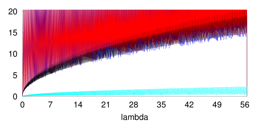
Memory usage graphs for the benchmarks are shown in Figure 10. In all the programs we can see that the curve corresponding to LGC (blue line) dips below the RGC curve (red line) during GC. The graphs also include the curve for reachable cells (black) and live cells (light-blue). These were obtained by forcing RGC to run at very high frequency. The curve for live cells were obtained by recording heap access times and post processing the data at the end of the program. Note that the size of an LGC cell is 1.16 times the size of a RGC cell as it potentially might have to store references to liveness DFA of closure arguments (if the cell is a closure).
As demonstrated by the gap between the red and the light-blue lines, a large number of cells which are unused by the program are still copied during RGC. LGC does a much better job of closing this gap but still falls short of the precision achieved by LGC in case of eager languages [6]. A major source of inefficiency in LGC is multiple traversals of already copied heap cells. Since LGC does not mark the heap cells after the first visit, the same cells can be repeatedly visited with different liveness states. We have mitigated this problem by implementing a heuristic which avoids revisiting closures and function arguments more than once.
7 Related work
The impact of liveness on the effectiveness of GC is investigated in [14]. They observe that liveness can significantly impact garbage collection, but only when it is interprocedural. As far as memory requirement is concerned, our paper demonstrates this observation.
There have been several attempts to use liveness analysis to improve GC for imperative languages. [20] presents a liveness analysis and uses the results for inserting nullifying statements in Java programs. In [29], temporal properties like liveness are checked against an automaton modeling heap accesses. Both these approaches are intraprocedural in scope.
In the space of functional languages, there are: rewriting methods such as deforestation [34, 12, 9], sharing analysis based reallocation [17], region based analysis [33], and insertion of compile-time nullifying statements [16, 21]. All compile-time marking approaches rely on an efficient and precise alias analysis and cannot provide significant improvement in its absence. The only work in the space of lazy languages seems to be [13] which touches upon only basic techniques of compile-time garbage marking, explicit deallocation and destructive allocation. An interesting approach suggested in [15] is to annotate the heap usage of first-order programs through linear types. The annotations are then used to serve memory requests through re-allocation. However, this requires the user to write programs in a specific way. Safe-for-space [5] approaches [10, 30] reduce the amount of heap used by a program by allocating closures in registers and through tail call optimizations. However, these approaches take care of only part of the problem addressed by our analysis as the program can still contain unused objects and closures that are reachable.
Simplifiers [24] are abstractly described as lightweight daemons that attach themselves to program data and, when activated, improve the efficiency of the program. Our liveness-based GC can be seen as an instance of a simplifier which is tightly coupled with garbage collectors. The approach that is closest to the method described in this paper is the liveness-based garbage collector implemented in [18, 6] and address eager languages. We extend this to handle lazy evaluation and closures.
8 Future work and conclusions
We have extended liveness-based GC to lazy languages and shown its benefit for a set of benchmark programs. We defined a liveness analysis of programs manipulating the heap and proved it correct with respect to a non-standard semantics that served as a specification of liveness. The result of the analysis is a set of grammars, whose membership question was shown to be undecidable. The grammars are therefore approximated by DFAs and used by the garbage collector to improve collection.
In addition to evaluated data, our collector also reclaims closures. For this, we had to modify the standard run-time representation of closures to carry liveness of its free variables and periodically update the liveness during execution time. As expected, our garbage collector reclaims more garbage and reduces memory requirement of programs. An additional benefit is that in spite of using a more expensive collector, the execution times remains comparable in most cases, and even improves for some programs.
The graphs show that even in lazy languages there are large amount of dead cells that can be collected early. In spite of collecting closures there still exists a gap between actual and perceived livenesses. Language features that could be introduced are higher-order functions and recursive lets. We believe that functions can be used to model recursive lets and this should be a simple extension to our liveness analysis. For higher-order we intend to use firstification techniques [22].
Orthogonally, we plan to improve the efficiency of the liveness-based garbage collector using heuristics such as limiting the depth of DFA, merging nearly-equivalent states and using better representation (for example BDDs [7]) and algorithms for automata manipulation. We also need to investigate the interaction of liveness with other collection schemes, such as incremental and generational collection. It might be interesting to use a mixed mode GC scheme which allows the costs of LGC to be amortized over several runs of RGC. In summary, we need to investigate ways to make liveness-based GC attractive for practical collectors.
References
- [1] An artificial garbage collection benchmark. http://www.hboehm.info/gc/gc_bench.html, Nov 2015. (Last Accessed).
- [2] Huffman encoding trees. https://mitpress.mit.edu/sicp/full-text/sicp/book/node41.html, Nov 2015. (Last Accessed).
- [3] NoFib: Haskell Benchmark Suite. http://git.haskell.org/nofib.git, Nov 2015. (Last accessed).
- [4] PLT Scheme Benchmark Suite. http://svn.plt-scheme.org/plt/trunk/collects/tests/, Nov 2015. (Last accessed).
- [5] A. W. Appel. Compiling with Continuations. Cambridge University Press, 2006.
- [6] R. Asati, A. Sanyal, A. Karkare, and A. Mycroft. Liveness-based garbage collection. In Compiler Construction - 23rd International Conference, CC 2014, Held as Part of the European Joint Conferences on Theory and Practice of Software, ETAPS 2014, Grenoble, France, April 5-13, 2014. Proceedings, pages 85–106, 2014.
- [7] R. E. Bryant. Graph-based algorithms for boolean function manipulation. IEEE Trans. Computers, 35(8):677–691, 1986.
- [8] M. M. T. Chakravarty, G. Keller, and P. Zadarnowski. A functional perspective on SSA optimisation algorithms. Electr. Notes Theor. Comput. Sci., 82(2):347–361, 2003.
- [9] O. Chitil. Type inference builds a short cut to deforestation. In Proceedings of the fourth ACM SIGPLAN International Conference on Functional Programming (ICFP ’99), Paris, France, September 27-29, 1999., pages 249–260, 1999.
- [10] W. D. Clinger. Proper tail recursion and space efficiency. In Proceedings of the ACM SIGPLAN ’98 Conference on Programming Language Design and Implementation (PLDI), Montreal, Canada, June 17-19, 1998, pages 174–185, 1998.
- [11] J. Fairbairn and S. Wray. Functional Programming Languages and Computer Architecture: Portland, Oregon, USA, September 14–16, 1987 Proceedings, chapter Tim: A simple, lazy abstract machine to execute supercombinators, pages 34–45. Springer Berlin Heidelberg, Berlin, Heidelberg, 1987.
- [12] A. J. Gill, J. Launchbury, and S. L. Peyton Jones. A short cut to deforestation. In Proceedings of the conference on Functional programming languages and computer architecture, FPCA 1993, Copenhagen, Denmark, June 9-11, 1993, pages 223–232, 1993.
- [13] G. W. Hamilton. Compile-time garbage collection for lazy functional languages. In Proceedings of the International Workshop on Memory Management, IWMM ’95, pages 119–144, London, UK, UK, 1995. Springer-Verlag.
- [14] M. Hirzel, A. Diwan, and J. Henkel. On the usefulness of type and liveness accuracy for garbage collection and leak detection. ACM Trans. Program. Lang. Syst., 24(6):593–624, 2002.
- [15] M. Hofmann and S. Jost. Static prediction of heap space usage for first-order functional programs. In Conference Record of POPL 2003: The 30th SIGPLAN-SIGACT Symposium on Principles of Programming Languages, New Orleans, Louisisana, USA, January 15-17, 2003, pages 185–197, 2003.
- [16] K. Inoue, H. Seki, and H. Yagi. Analysis of functional programs to detect run-time garbage cells. ACM Trans. Program. Lang. Syst., 10(4):555–578, 1988.
- [17] S. B. Jones and D. Le Métayer. Compile-time garbage collection by sharing analysis. In Proceedings of the Fourth International Conference on Functional Programming Languages and Computer Architecture, FPCA ’89, pages 54–74, New York, NY, USA, 1989. ACM.
- [18] A. Karkare, U. P. Khedker, and A. Sanyal. Liveness of heap data for functional programs. In Heap Analysis and Verification, HAV 2007, a satellite workshop of European Joint Conferences on Theory and Practice of Software, ETAPS 2007, March 25, 2007, Braga, Portugal, 2007.
- [19] A. Karkare, A. Sanyal, and U. P. Khedker. Effectiveness of garbage collection in MIT/GNU scheme. CoRR, abs/cs/0611093, 2006.
- [20] U. P. Khedker, A. Sanyal, and A. Karkare. Heap reference analysis using access graphs. ACM Trans. Program. Lang. Syst., 30(1), 2007.
- [21] O. Lee, H. Yang, and K. Yi. Static insertion of safe and effective memory reuse commands into ml-like programs. Sci. Comput. Program., 58(1-2):141–178, 2005.
- [22] N. Mitchell and C. Runciman. Losing functions without gaining data: another look at defunctionalisation. In Proceedings of the 2nd ACM SIGPLAN Symposium on Haskell, Haskell 2009, Edinburgh, Scotland, UK, 3 September 2009, pages 13–24, 2009.
- [23] M. Mohri and M.-J. Nederhof. Regular approximation of context-free grammars through transformation. In Robustness in Language and Speech Technology. Kluwer Academic Publishers, 2000.
- [24] M. E. O’Neill and F. W. Burton. Smarter garbage collection with simplifiers. In Proceedings of the 2006 workshop on Memory System Performance and Correctness, San Jose, California, USA, October 11, 2006, pages 19–30, 2006.
- [25] S. L. Peyton Jones. The Implementation of Functional Programming Languages. Prentice-Hall, 1987.
- [26] N. Röjemo and C. Runciman. Lag, drag, void and use - heap profiling and space-efficient compilation revisited. In Proceedings of the 1996 ACM SIGPLAN International Conference on Functional Programming (ICFP ’96), Philadelphia, Pennsylvania, May 24-26, 1996., pages 34–41, 1996.
- [27] R. Shaham, E. K. Kolodner, and S. Sagiv. Heap profiling for space-efficient Java. In Proceedings of the 2001 ACM SIGPLAN Conference on Programming Language Design and Implementation (PLDI), Snowbird, Utah, USA, June 20-22, 2001, pages 104–113, 2001.
- [28] R. Shaham, E. K. Kolodner, and S. Sagiv. Estimating the impact of heap liveness information on space consumption in Java. In Proceedings of The Workshop on Memory Systems Performance (MSP 2002), June 16, 2002 and The International Symposium on Memory Management (ISMM 2002), June 20-21, 2002, Berlin, Germany, pages 171–182, 2002.
- [29] R. Shaham, E. Yahav, E. K. Kolodner, and S. Sagiv. Establishing local temporal heap safety properties with applications to compile-time memory management. In Static Analysis, 10th International Symposium, SAS 2003, San Diego, CA, USA, June 11-13, 2003, Proceedings, pages 483–503, 2003.
- [30] Z. Shao and A. W. Appel. Efficient and safe-for-space closure conversion. ACM Trans. Program. Lang. Syst., 22(1):129–161, 2000.
- [31] O. Shivers. Control-flow analysis in scheme. In Proceedings of the ACM SIGPLAN’88 Conference on Programming Language Design and Implementation (PLDI), Atlanta, Georgia, USA, June 22-24, 1988, pages 164–174, 1988.
- [32] S. Thomas. Garbage collection in shared-environment closure reducers: Space-efficient depth first copying using a tailored approach. Information Processing Letters, 56(1):1 – 7, 1995.
- [33] M. Tofte and L. Birkedal. A region inference algorithm. ACM Trans. Program. Lang. Syst., 20(4):724–767, 1998.
- [34] P. Wadler. Deforestation: Transforming programs to eliminate trees. In ESOP ’88, 2nd European Symposium on Programming, Nancy, France, March 21-24, 1988, Proceedings, pages 344–358, 1988.
Appendix A Complete Minefield Semantics
| Premise | Transition | Rule name |
| const | ||
| cons | ||
| car-bang | ||
| car-select | ||
| car-clo | ||
| car-1-clo | ||
| or | prim-bang | |
| prim-add | ||
| prim-1-clo | ||
| prim-2-clo | ||
| funcall | ||
| , is a new location | where | let |
| if-bang | ||
| if-true | ||
| if-false | ||
| if-clo | ||
| return-bang | ||
| return-whnf | ||
| return-clo |