Valid parameter space of a bivariate Gaussian Markov random field with a generalized block-Toeplitz precision matrix

The analysis of large datasets with complicated spatio-temporal dependence structures is among the major challenges in modern statistics. With respect to this, sophisticated models are used in order to capture such dependencies. In [2, 29], an overview of these models is provided. In addition, computational efficiency is crucial, since the size of the datasets available to the scientific community has been growing steadily over the years.

A broad class of the models currently in use in spatial statistics are Gaussian latent models, discussed in full detail in [23]. The case of observations on a lattice is of particular interest. Several case studies are discussed, for instance in [22], and some related modeling and computational challenges are covered in [9]. In the case of Gaussian observations $\boldsymbol{y}$ over a (regular) lattice, a prototypical model is

where $\boldsymbol{x}$ are known covariates. In the Bayesian setting (see, e.g., [8]), prior distributions on the (hyper) parameters $\boldsymbol{\beta},\boldsymbol{\theta}$, and $\sigma$ are to be specified. In the previous model, the layer (1a) accounts for the fact that the data $\boldsymbol{y}$ is assumed to be independent at different locations on the lattice, conditionally on a linear term $\boldsymbol{x}^{\top}\boldsymbol{\beta}$ and a latent field $\boldsymbol{z}$. The layer (1b) models complicated spatial dependencies through the parameter $\boldsymbol{\theta}$. In this context, the spatial correlation structure can be specified through the off-diagonal non-zero elements of the precision matrix $\boldsymbol{Q}(\boldsymbol{\theta})$ of the random vector $\boldsymbol{z}$ (see, e.g., [22] for details). Equivalently, the model (1) can be specified in terms of the expected value of the Gaussian full-conditional distribution at each location, in the framework of a conditional autoregressive (CAR) model. The CAR models and their importance in spatial statistics are well-known and discussed in [17].

The ease of interpretability of the model (1) comes at a price. In the applications, at least three crucial aspects are to be considered. Depending on the structure and the size of the precision matrix $\boldsymbol{Q}(\boldsymbol{\theta})$, it can be computationally intensive to evaluate quadratic forms and log-determinants involving such matrices. Of course, this can lead to high computational costs when, for instance, implementing a Markov Chain Monte Carlo (MCMC) sampler for large datasets (see, e.g., [7]). It is then necessary to develop efficient computational strategies in order to evaluate the above-mentioned quantities. In the literature, the case of a univariate field over a regular lattice of size $n=n_{1}\times n_{2}$ with a block-Toeplitz precision is thoroughly covered. The main idea, discussed in [17], is to consider a lattice with toroidal boundary conditions. Under this approximation, the precision matrix becomes block-circulant and very efficient algorithms for the latter class of matrices can be used. They are based on the (multidimensional) fast Fourier transform (FFT), discussed in full detail in [3]. The third aspect that has to be considered is to determine the valid parameter space for the model (1), namely the set of parameters for which the precision matrix $\boldsymbol{Q}(\boldsymbol{\theta})$ is (semi) positive-definite. The importance of this task is pointed out, for instance in [6, 22]. Once again, the solution of this problem is essential if we want to implement a MCMC sampler or an optimization algorithm for the maximum likelihood estimation for a model of the form (1). In the former case, we need to know the set over which we can impose a prior distribution on $\boldsymbol{\theta}$, whereas in the latter case the domain of the function to be optimized must be determined. To our knowledge, in the literature, only specific precision matrix structures (block-Toeplitz matrices, discussed in [22], and block-circulant, e.g., in [32]), and univariate fields (e.g., in [26]) are covered. The case of bivariate fields, on the contrary, was not analytically explored. So far, only approaches aimed at determining analytically tractable subsets of the domain, such as the diagonal dominance criterion, were considered, for example in [22]. The obtained results were, however, unsatisfactory in terms of coverage of the whole valid parameter space. Apart from this, the determination of the parameter space relied on brute-force “trial-and-error” approaches, based on the fact that a Hermitian matrix is positive-definite if and only if it admits a unique Cholesky factorization (see [6] for the details). However, these techniques are computationally expensive.

In this paper, we consider the model introduced in [25] to analyze bivariate data coming from several regional climate models (RCMs). In particular, we focus on the associated bivariate GMRF, which is in the form of the layer (1b). It depends on seven real parameters, namely $\phi,\rho_{11},\rho_{12},\rho_{21},\rho_{22},\tau_{1}$, and $\tau_{2}$. These in turn stem from the layer decomposition introduced in [25], which is an approach to interpret a multivariate GMRF as an instance of univariate GMRF. The main idea behind this concept is to work with one layer for each variable of interest. In this context, $\phi$ corresponds to within-location variability, whereas $\rho_{11}$ and $\rho_{22}$ describe within-variable variability. Furthermore, $\rho_{12}$ and $\rho_{21}$ account for the cross-location variability. These parameters correspond to the coefficients of a linear combination through which the expected values of the aforementioned full-conditional distributions are defined. Finally, $\tau_{1}^{2}$ and $\tau_{2}^{2}$ are the marginal variances of these bivariate distributions. Due to the different nature of these parameters, it natural to set the following:

which induce the precision matrix $\boldsymbol{Q}_{n_{1},n_{2}}(\boldsymbol{\theta},\boldsymbol{\tau})\in\mathbb{R}^{2n\times 2n}$.

The main goal of this paper is to provide asymptotically closed-form expressions of the valid parameter space, namely

In the previous definition, we assumed strictly positive-definite precision matrices. Although in this paper we will mainly focus on a specific bivariate GMRF, one important goal will be to provide a methodology that can be extended to multivariate GMRFs, whose precision matrix has a generalized Toeplitz matrix for which no analytic results for the eigenvalues can be obtained. In other words, the aim of our methodology is to overcome the aforementioned lack of theoretical results for multivariate GMRFs.

The structure of the paper follows. In Section 2, we will briefly describe the model outlined in [25] and enumerate some preliminary results, which will be necessary later. In addition, extending the work presented in [11], we will develop a toroidal boundary condition approximation: $\widetilde{\boldsymbol{Q}}_{n_{1},n_{2}}(\boldsymbol{\theta},\boldsymbol{\tau})$ of $\boldsymbol{Q}_{n_{1},n_{2}}(\boldsymbol{\theta},\boldsymbol{\tau})$ in order to characterize the domain (2) through

The asymmetry in the parameters $\rho_{12}$ and $\rho_{21}$, which was introduced in [24, 25] in order to better describe spatial dependence, for instance in the aforementioned RCM data, will play a central role. The importance and feasibility of our approach in the applications will be further discussed. In Section 3, we will state and formally prove our main result, namely the convergence—in a suitable sense—of $\widetilde{\boldsymbol{\Theta}}_{n_{1},n_{2}}$ to $\boldsymbol{\Theta}_{n_{1},n_{2}}$. This result will highlight the fact that considering a regular grid with toroidal boundary conditions is not only useful to evaluate log-determinants and quadratic forms but is also useful, for instance, to efficiently sample a prior distribution defined over the set (2). This in turn improves what is discussed in [22], where a regular grid without boundary conditions is embedded in a bigger grid with toroidal boundary conditions. The limitations of other known convergence results for this problem (e.g., the weak convergence of sequences of matrices discussed in [11], the Szegö theorem covered in [12], etc.) will also be discussed. In Section 4, we will implement a thorough simulation study aimed at numerically assessing the rate of convergence of our approximation. We will additionally discuss some related aspects, which are important in the applications. Finally, in Section 5, we will provide some conclusive remarks.

We briefly outline the model introduced in [25] in order to analyze bivariate data over a regular lattice of size $n=n_{1}\times n_{2}$, with particular emphasis on the structure of the precision matrix of the latent field $\boldsymbol{z}$ of equation (1b), which will play a crucial role in what follows. Up to a permutation of the rows and columns, the precision matrix of size $2n\times 2n$ can be rewritten as follows:

where $\boldsymbol{\tau}_{1}=\operatorname{diag}(\tau_{1})\in\mathbb{R}^{n\times n}$, $\boldsymbol{\tau}_{2}=\operatorname{diag}(\tau_{2})\in\mathbb{R}^{n\times n}$ and $\operatorname{diag}(x)=x\,\boldsymbol{I}$. The four blocks of the form $\boldsymbol{T}_{n_{1},n_{2}}(\cdot)$ in the previous equation have size $n\times n$ and are block-Toeplitz, with the following structure:

where

Then, $\boldsymbol{T}_{n_{1},n_{2}}(\rho_{11},1,\rho_{11})=\boldsymbol{T}_{n_{1},n_{2}}(\rho_{22},1,\rho_{22})$ if and only if $\rho_{11}=\rho_{22}$. This means that $\boldsymbol{Q}_{n_{1},n_{2}}(\boldsymbol{\theta},\boldsymbol{\tau})$ is in general not block-Toeplitz. This structure generalizes what is discussed in [14, 22], where the precision (or, in turn, the variance-covariance) matrix is block-Toeplitz. Our precision matrix is also sparse, and the non-zero entries pattern is shown in the left panel of Figure 1. It can be shown that $\boldsymbol{Q}_{n_{1},n_{2}}(\boldsymbol{\theta},\boldsymbol{\tau})$ has at most $20n_{1}n_{2}-8n_{1}-8n_{2}\in\Theta(n)$ non-zero entries. In this paper, we use the big theta notation, namely $f(n)\in\Theta(g(n))$ if and only if $f(n)$ is eventually bounded from both above and below by $g(n)$.

Recall that the first goal of this study is to characterize the valid parameter space (2). In the literature (e.g., in [22]) the diagonal dominance criterion is used in order to determine analytically tractable subsets. More precisely, it is well-known that an Hermitian matrix $\boldsymbol{A}\in\mathbb{C}^{n\times n}$ such that $\big|(\boldsymbol{A})_{i}^{i}\big|\geq\sum_{j\neq i}\big|(\boldsymbol{A})_{i}^{j}\big|$, for all $i=1,2,\dots,n$, is semipositive-definite (a formal proof of this statement is provided in [13]). However, the converse does not hold in general. In order to highlight the importance of the convergence result that we will discuss in the next section, we will preliminarily deal with the limitations of the diagonal dominance criterion for the precision matrix (4). With respect to this, we uniformly drew 500,000 values of $\boldsymbol{\theta}$ belonging to the valid parameter space (2) with $n_{1}=n_{2}=100$. Among these, we determined the ones also satisfying the diagonal dominance criterion. The ratio between the latter and the former was 0.1288. This rate of coverage is clearly unsatisfactory and agrees with [22] for univariate GMRFs. In addition, in order to attain a partial understanding of the geometrical structure of the set (2), we additionally drew uniformly four values of $(\phi,\rho_{11},\rho_{22})^{\top}$ from the set (2). For each of them, we uniformly sampled 10,000 values of $(\rho_{12},\rho_{21})^{\top}$ such that $(\phi,\rho_{11},\rho_{22},\rho_{12},\rho_{21})^{\top}$ belong to (2). We chose this approach since it is relatively easy to devise closed-form bounds for each of the parameters $\phi,\rho_{11}$, and $\rho_{22}$, whereas the same does not hold for $\rho_{12}$ and $\rho_{21}$. The obtained results are displayed in Figure 2. The blue points correspond to values of the parameters belonging to the set (2). The ones also satisfying the diagonal dominance criterion are highlighted in orange. Several features are striking. First, there are values of $(\phi,\rho_{11},\rho_{22})^{\top}$ for which the diagonal dominance criterion provides no coverage. Even when it does, the coverage rate is clearly unsatisfactory. Second, the region determined by this criterion is symmetric around the origin, while the region determined by the valid points is generally not symmetric around this point. In other words, the diagonal dominance criterion is not able to capture the geometrical structure of the valid parameter space (2).

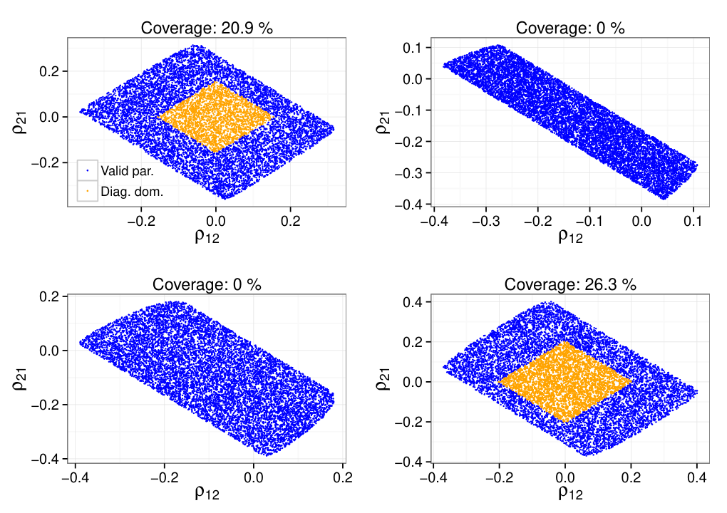
As a consequence, we need to resort to a different approach to describe the valid parameter space (2). The latter problem is equivalent to determining the values of $\boldsymbol{\theta}$ and $\boldsymbol{\tau}$ such that the minimum eigenvalue of $\boldsymbol{Q}_{n_{1},n_{2}}(\boldsymbol{\theta},\boldsymbol{\tau})$ is strictly positive. Consequently, we will focus on the spectrum of $\boldsymbol{Q}_{n_{1},n_{2}}(\boldsymbol{\theta},\boldsymbol{\tau})$, which will be denoted with $\sigma(\boldsymbol{Q}_{n_{1},n_{2}}(\boldsymbol{\theta},\boldsymbol{\tau}))$. In addition, we will adhere to the convention of enumerating the eigenvalues in decreasing order, namely $\lambda_{1}(\boldsymbol{Q}_{n_{1},n_{2}}(\boldsymbol{\theta},\boldsymbol{\tau}))\geq\lambda_{2}(\boldsymbol{Q}_{n_{1},n_{2}}(\boldsymbol{\theta},\boldsymbol{\tau}))\geq\dots\geq\lambda_{2n}(\boldsymbol{Q}_{n_{1},n_{2}}(\boldsymbol{\theta},\boldsymbol{\tau}))$. From equation (4), it is clear that $\boldsymbol{Q}_{n_{1},n_{2}}(\boldsymbol{\theta},\boldsymbol{\tau})$ is positive-definite only if $\tau_{1},\tau_{2}>0$. Henceforth, we will only consider the inner matrix of equation (4), which depends only on $\boldsymbol{\theta}$. Moreover, we will drop the dependence on $\boldsymbol{\tau}$ in order to keep the notation as straightforward as possible.

No closed-form formulas for the eigenvalues of $\boldsymbol{Q}_{n_{1},n_{2}}(\boldsymbol{\theta})$ are available. More specifically, only results for banded block-Toeplitz matrices are discussed (see, e.g., [19]). In the special case $\rho_{12}=\rho_{21}$, it can be shown that there exists an orthogonal matrix $\boldsymbol{V}_{n_{1},n_{2}}\in\mathbb{R}^{n\times n}$ not depending on $\boldsymbol{\theta}$ such that

where $\boldsymbol{\Lambda}_{ij}(\boldsymbol{\theta})$ is a diagonal matrix whose diagonal elements are the eigenvalues of the four $n\times n$ symmetric blocks into which the inner matrix of precision (4) is partitioned. In other words, the latter are simultaneously diagonalizable through $\boldsymbol{V}_{n_{1},n_{2}}$. This property is a consequence of the fact that

as also observed in [26] when dealing with univariate GMRFs with a second-order neighborhood. Up to a permutation of the rows and columns, the right-hand-side of the equation (6) is a symmetric block-diagonal matrix whose diagonal blocks have size $2\times 2$. At this point, the determination of $\sigma(\boldsymbol{Q}_{n_{1},n_{2}}(\boldsymbol{\theta}))$ is straightforward.

In the general case in which $\rho_{12}\neq\rho_{21}$, the four $n\times n$ blocks of the precision (4) are not simultaneously diagonalizable. Therefore, the spectrum cannot be readily devised. The main idea to overcome this lack of analytical results is to introduce a perturbed precision matrix $\widetilde{\boldsymbol{Q}}_{n_{1},n_{2}}(\boldsymbol{\theta})\in\mathbb{R}^{2n\times 2n}$, which can be partitioned into four $n\times n$ blocks which are block-circulant. This will extend the approach used in [11] and is equivalent to toroidal boundary conditions on the underlying lattice.

The perturbation is carried out as follows. Bearing in mind how the function $\boldsymbol{T}_{n_{1},n_{2}}(\cdot)$ was defined in (5), we see that all but its sub-blocks on the main diagonal are already circulant. On the other hand, the sub-blocks on the main diagonal are by construction tridiagonal and hence can be made circulant in a natural way as follows:

We explicitly point out that this method of turning a tridiagonal (more generally, non-circulant Toeplitz) matrix into a circulant one is not unique. In the literature, several approaches are discussed (see, e.g., [4]). However, in our case, a simulation study provided strong empirical evidence of the fact that more sophisticated approaches are advantageous only for small choices of the grid size $n$. As we are interested in an asymptotic description of $\sigma(\boldsymbol{Q}_{n_{1},n_{2}}(\boldsymbol{\theta}))$, we decided to stick to the natural approach. We then set:

It follows that the blocks $\boldsymbol{C}_{n_{1},n_{2}}(\cdot)$ are block-circulant matrices of size $n$. Similarly to what was observed above for $\boldsymbol{Q}_{n_{1},n_{2}}(\boldsymbol{\theta})$, the perturbed matrix (7) is block-circulant if and only if $\rho_{11}=\rho_{22}$.

Now, let $\Delta\boldsymbol{Q}_{n_{1},n_{2}}(\boldsymbol{\theta})=\boldsymbol{\widetilde{Q}}_{n_{1},n_{2}}(\boldsymbol{\theta})-\boldsymbol{{Q}}_{n_{1},n_{2}}(\boldsymbol{\theta})$ be the perturbation matrix (see the right panel of Figure 1 to inspect its structure). It has at most $8(n_{1}+n_{2})\in\Theta(n_{1}+n_{2})$ non-zero entries. This implies that the limit for $n_{1},n_{2}\to+\infty$ of the ratio between the number of non-zero elements of $\boldsymbol{Q}_{n_{1},n_{2}}(\boldsymbol{\theta})$ and of $\Delta\boldsymbol{Q}_{n_{1},n_{2}}(\boldsymbol{\theta})$ is infinite. This property will be crucial in Lemma 4, when we will prove our main convergence result. Apart from this, the trace of $\Delta\boldsymbol{Q}_{n_{1},n_{2}}(\boldsymbol{\theta})$ is zero, and its rank is greater than zero, unless ${\rho_{11}=\rho_{12}=\rho_{21}=\rho_{22}=0}$. This implies that $\Delta\boldsymbol{Q}_{n_{1},n_{2}}(\boldsymbol{\theta})$ is an indefinite matrix; namely that it has both strictly positive and strictly negative eigenvalues. Explicit formulas for these eigenvalues can be symbolically derived, as only their algebraic multiplicity changes when $n$ grows, but they are not reported here, as they are rather complicated and not necessary for what follows. It is also important to point out that the Weyl’s inequalities [31] imply that

These bounds are however too loose to approximate the valid parameter space (2).

We now turn to the study of $\sigma(\widetilde{\boldsymbol{Q}}_{n_{1},n_{2}}(\boldsymbol{\theta}))$, which will allow us to characterize the set (3). In the case of a block-circulant of size $n_{1}\,n_{2}\times n_{1}\,n_{2}$ whose sub-blocks have size $n_{1}\times n_{1}$, the eigenvalues can be efficiently computed using the bidimensional FFT, with a computational complexity of $\Theta(n_{1}\,n_{2}\,\log{(n_{1}\,n_{2})})$, as discussed in [3]. For the perturbed precision (7), we obtain:

where $\imath$ is the imaginary unit, $I=\{0,1,2,\dots,n_{2}-1\}$ and $J=\{0,1,2,\dots,n_{1}-1\}$. This result readily provides the eigenvalues of the four $n\times n$ blocks of (7). In particular, the eigenvalues of the two diagonal blocks are real, since the latter are by construction symmetric. For instance, for the top-left block of (7) it holds that

We are now ready to explicitly derive $\sigma(\widetilde{\boldsymbol{Q}}_{n_{1},n_{2}}(\boldsymbol{\theta}))$. Let

where, after having set $\omega=\exp{(-2\pi\imath/n)}$:

and $\boldsymbol{P}_{n}^{(m)}\in\mathbb{R}^{2mn\times 2mn}$ is a suitable permutation matrix. Of course, $\boldsymbol{F}_{n}$ is the normalized discrete Fourier transform (DFT) matrix, discussed in full detail in [3]. Closed-form expression for $\boldsymbol{U}_{n_{1},n_{2}}$ can be obtained, but once again they are not reported because they are not strictly necessary for what follows. It will suffice to observe that its non-zero entries are generally complex, with absolute value $1/{\sqrt{n_{1}n_{2}}}$. The non-zero entry pattern is displayed in Figure 3.

In addition, $\boldsymbol{U}_{n_{1},n_{2}}$ is by construction unitary, does not depend on $\boldsymbol{\theta}$, and is such that

where ^∗ denotes the complex conjugate operator, $i\in I,j\in J$ and $\widetilde{\lambda}_{i,j}^{(n)}(x,y,z)$ is the $(i,j)$th- eigenvalue of the block-circulant block $\boldsymbol{C}_{n_{1},n_{2}}(x,y,z)$ of size $n$ belonging to the matrix (7). From the previous result, we finally obtain closed-form expressions for $\sigma(\widetilde{\boldsymbol{Q}}_{n_{1},n_{2}}(\boldsymbol{\theta}))$, namely

From equations (10) and (11), several important results follow. First, a unitary matrix $\boldsymbol{V}_{n_{1},n_{2}}(\boldsymbol{\theta})$ of size $2n\times 2n$ exists, such that the perturbed precision matrix $\widetilde{\boldsymbol{Q}}_{n_{1},n_{2}}(\boldsymbol{\theta})$ can be diagonalized by the transformation $\boldsymbol{U}_{n_{1},n_{2}}\boldsymbol{V}_{n_{1},n_{2}}(\boldsymbol{\theta})$. It clearly follows that the columns of $\boldsymbol{U}_{n_{1},n_{2}}\boldsymbol{V}_{n_{1},n_{2}}(\boldsymbol{\theta})$ are eigenvectors of $\widetilde{\boldsymbol{Q}}_{n_{1},n_{2}}(\boldsymbol{\theta})$. In addition, each column of $\boldsymbol{V}_{n_{1},n_{2}}(\boldsymbol{\theta})$ contains exactly two non-zero entries. They correspond to an eigenvector of one of the $n_{1}n_{2}$ blocks of size $2\times 2$ of equation (11). This readily provides an estimate of the absolute value of the entries of $\boldsymbol{U}_{n_{1},n_{2}}\boldsymbol{V}_{n_{1},n_{2}}(\boldsymbol{\theta})$. Without loss of generality, we assume that the two non-zero entries of $(\boldsymbol{V}_{n_{1},n_{2}}(\boldsymbol{\theta}))^{m}$ are its two first components. Then,

where $l,m=1,2,\dots,2n$. The first inequality holds due to the triangular inequality and the above stated norm of the entries of $\boldsymbol{U}_{n_{1},n_{2}}$, while the second one holds since $\boldsymbol{V}_{n_{1},n_{2}}(\boldsymbol{\theta})$ is unitary and hence $|(\boldsymbol{V}_{n_{1},n_{2}}(\boldsymbol{\theta}))_{1}^{m}|^{2}+|(\boldsymbol{V}_{n_{1},n_{2}}(\boldsymbol{\theta}))_{2}^{m}|^{2}=1$.

To summarize, in this section, we solved the analogous of problem (2) for the perturbed matrix (7). In other words, we found closed-form expressions for the set (3). In fact, it is enough to impose that all $2n$ eigenvalues (12) are strictly positive. The next step is to prove asymptotically that $\boldsymbol{Q}_{n_{1},n_{2}}(\boldsymbol{\theta})$ is positive-definite if and only if this property holds for $\widetilde{\boldsymbol{Q}}_{n_{1},n_{2}}(\boldsymbol{\theta})$.

We conclude this section by discussing the importance of the knowledge of the eigenvalues (12) in the applications. The main result in this context is that we can test whether $\boldsymbol{\theta}$ belongs to the perturbed valid parameter space (3) by numerically checking that the eigenvalues (12) evaluated at $\boldsymbol{\theta}$ are positive. Once again, in the next section, we will show that this task is asymptotically equivalent to testing whether $\boldsymbol{\theta}$ belongs to (2). Here, we highlight the usefulness of the closed-form expressions (12) in the applications from a general perspective. A uniform prior distribution on $\boldsymbol{\theta}$ has the following form:

where $\boldsymbol{1}(\cdot)$ is the indicator function. We need to evaluate all the $n$ terms of the form $\boldsymbol{1}(\lambda_{i}(\boldsymbol{Q}_{n_{1},n_{2}}(\boldsymbol{\theta}))>0)$ because the analytical expression of $\lambda_{2n}(\boldsymbol{Q}_{n_{1},n_{2}}(\boldsymbol{\theta}))$ depends on complicated conditions on the components of $\boldsymbol{\theta}$. Through equation (12), this task can be accomplished with complexity $\Theta(n)$. The gain in computational efficiency is substantial. We benchmarked our approach against using the R package spam [6], which provides numerical routines for sparse matrix algebra. We considered three grid sizes, namely $100\times 100$, $200\times 200$, and $300\times 300$. We observe that, if $\boldsymbol{\theta}$ induces a positive-definite precision matrix, it is then necessary to construct the latter (for instance, to evaluate the corresponding log-likelihood function), although our method in principle does not require this construction. On the contrary, if our approach determines that $\boldsymbol{\theta}$ does not belong to (2), then it is not necessary to construct the corresponding precision, as the drawn $\boldsymbol{\theta}$ is to be discarded. In order to meaningfully assess both scenarios, for each of the aforementioned grid sizes, we drew 50 values of $\boldsymbol{\theta}$ belonging to the valid parameter (2) and 50 values not belonging to this domain and recorded the correspondent computational times. For each of these 100 parameter values, we recorded the computational time in both spam and our approach. This task was accomplished through the R package microbenchmark [18]. In the case of the 50 valid parameter values and for the three considered grid sizes, the median of the recorded computational times for spam was 2.6, 5.9, and 11.6 times the median obtained with our approach. The performance of our approach clearly improves when the grid size increases. In the case of the non-valid parameters, for which it was not necessary to construct the precision matrix, the median of spam was 40.6, 84.7, and 208.7 times the median of our approach. These timings can be further improved by exploiting the structure of the set (3), which is analytically provided by equation (12). It can be shown that, if we assume without loss of generality that $n_{1}<n_{2}$, the eigenvalues (12) attain exactly $n_{2}$ local minima. It follows that we only need to evaluate $n_{2}$ elements of the form $\boldsymbol{1}(\lambda_{i}(\boldsymbol{Q}_{n_{1},n_{2}}(\boldsymbol{\theta}))>0)$ in order to test whether $\boldsymbol{\theta}$ belongs to the set (3). From all the above-mentioned results, it is striking that our method outperforms the numerical routines of spam. This property is crucial, for instance, in an MCMC sampler, where the task of determining whether $\boldsymbol{\theta}$ is valid is usually repeated hundreds of thousands of times. Further aspects of our methodology are discussed in Section 5.

In the previous section, the perturbation $\widetilde{\boldsymbol{Q}}_{n_{1},n_{2}}(\boldsymbol{\theta})$ of $\boldsymbol{Q}_{n_{1},n_{2}}(\boldsymbol{\theta})$ was introduced. We will now formally prove our main result.

The previous result implies that, asymptotically, $\boldsymbol{Q}_{n_{1},n_{2}}(\boldsymbol{\theta})$ is positive-definite if and only if this property holds for $\widetilde{\boldsymbol{Q}}_{n_{1},n_{2}}(\boldsymbol{\theta})$.

First, we provide evidence of its novelty with respect to what is discussed in the literature in the following.

In order to prove Theorem 1, we preliminarily recall that

where $\langle\cdot,\cdot\rangle$ is the Euclidean inner product on $\mathbb{C}^{2n}$ and $\|\cdot\|$ is the correspondent induced norm. These results can be straightforwardly proved by diagonalizing the matrices ${\boldsymbol{Q}}_{n_{1},n_{2}}(\boldsymbol{\theta})$ and $\widetilde{\boldsymbol{Q}}_{n_{1},n_{2}}(\boldsymbol{\theta})$, respectively. In what follows, we will denote with $\boldsymbol{v}_{n_{1},n_{2}}(\boldsymbol{\theta})$ and $\boldsymbol{u}_{n_{1},n_{2}}(\boldsymbol{\theta})$ a solution of (14) and (15), respectively. They are eigenvectors associated with the eigenvalues $\lambda_{2n}({\boldsymbol{Q}}_{n_{1},n_{2}}(\boldsymbol{\theta}))$ and $\lambda_{2n}(\widetilde{\boldsymbol{Q}}_{n_{1},n_{2}}(\boldsymbol{\theta}))$, respectively. Based on equation (12) and (13), the following lemmas can be shown.

References

- [1] Aune, E., Eidsvik, J., and Pokern, Y. (2013). Iterative numerical methods for sampling from high dimensional Gaussian distributions. Statistics and Computing, 23, 501–521, doi:10.1007/s11222-012-9326-8.
- [2] Banerjee, S., Carlin, B. P., and Gelfand, A. E. (2004). Hierarchical Modeling and Analysis for Spatial Data. Chapman & Hall/CRC, Boca Raton, London.
- [3] Bracewell, R. (1978). The Fourier Transform and its Applications. McGraw-Hill Kogakusha, Ltd., Tokyo, second edition.
- [4] Chan, R. H. (1989). The spectrum of a family of circulant preconditioned Toeplitz systems. SIAM Journal on Numerical Analysis, 26, 503–506, doi:10.1137/0726029.
- [5] Dubes, R. and Jain, A. (1989). Random field models in image analysis. Journal of Applied Statistics, 16, 131–164, doi:10.1080/02664768900000014.
- [6] Furrer, R. and Sain, S. R. (2010). spam: A sparse matrix R package with emphasis on MCMC methods for Gaussian Markov random fields. Journal of Statistical Software, 36, 1–25, doi:10.18637/jss.v036.i10.
- [7] Gamerman, D. (1997). Markov Chain Monte Carlo: Stochastic Simulation for Bayesian Inference. Chapman & Hall/CRC Texts in Statistical Science. Taylor & Francis.
- [8] Gelman, A., Carlin, J., Stern, H., Dunson, D., Vehtari, A., and Rubin, D. (2013). Bayesian Data Analysis, Third Edition. Chapman & Hall/CRC Texts in Statistical Science. Taylor & Francis.
- [9] Gerber, F. and Furrer, R. (2015). Pitfalls in the implementation of Bayesian hierarchical modeling of areal count data: An illustration using BYM and Leroux models. Journal of Statistical Software, 63, 1–32, doi:10.18637/jss.v063.c01.
- [10] Gowda, M. S. and Tao, J. (2011). The Cauchy interlacing theorem in simple Euclidean Jordan algebras and some consequences. Linear and Multilinear Algebra, 59, 65–86, doi:10.1080/03081080903346425.
- [11] Gray, R. M. (2006). Toeplitz and circulant matrices: A review. Foundations and Trends in Communications and Information Theory, 2, 155–239, doi:10.1561/0100000006.
- [12] Grenander, U. and Szegö, G. (1984). Toeplitz Forms and their Applications. Chelsea Pub. Co., New York.
- [13] Horn, R. A. and Johnson, C. R., editors (1986). Matrix Analysis. Cambridge University Press, New York, NY, USA.
- [14] Kent, J. T. and Mardia, K. V. (1996). Spectral and circulant approximations to the likelihood for stationary Gaussian random fields. Journal of Statistical Planning and Inference, 50, 379–394, doi:10.1016/0378-3758(95)00065-8.
- [15] Kozintsev, B. (1999). Computations with Gaussian Random Fields. PhD thesis, Institute for Systems Research, University of Maryland. Cambridge University Press.
- [16] Lanczos, C. (1950). An iterative method for the solution of the eigenvalue problem of linear differential and integral operators. Journal of Research of the National Bureau of Standards, 45, 255–282, doi:10.6028/jres.045.026.
- [17] Mardia, K. V. (1988). Multi-dimensional multivariate Gaussian Markov random fields with application to image processing. Journal of Multivariate Analysis, 24, 265 – 284, doi:10.1016/0047-259X(88)90040-1.
- [18] Mersmann, O., Beleites, C., Hurling, R., and Friedman, A. (2015). Package ‘microbenchmark’. R package version 1.4-2.1.
- [19] Miranda, M. and Tilli, P. (2000). Asymptotic spectra of Hermitian block Toeplitz matrices and preconditioning results. SIAM Journal on Matrix Analysis and Applications, 21, 867–881, doi:10.1137/S0895479896313036.
- [20] Noschese, S., Pasquini, L., and Reichel, L. (2013). Tridiagonal Toeplitz matrices: properties and novel applications. Numerical Linear Algebra with Applications, 20, 302–326, doi:10.1002/nla.1811.
- [21] Qiu, Y., Mei, J., and authors of the ARPACK library. See file AUTHORS for details. (2014). rARPACK: R wrapper of ARPACK for large scale eigenvalue/vector problems, on both dense and sparse matrices. R package version 0.7-0.
- [22] Rue, H. and Held, L. (2005). Gaussian Markov Random Fields: Theory and Applications, volume 104 of Monographs on Statistics and Applied Probability. Chapman & Hall, London.
- [23] Rue, H., Martino, S., and Chopin, N. (2009). Approximate Bayesian inference for latent Gaussian models by using integrated nested Laplace approximations. Journal of the Royal Statistical Society: Series B (Statistical Methodology), 71, 319–392, doi:10.1111/j.1467-9868.2008.00700.x.
- [24] Sain, S. R. and Cressie, N. (2007). A spatial model for multivariate lattice data. Journal of Econometrics, 140, 226–259, doi:10.1016/j.jeconom.2006.09.010.
- [25] Sain, S. R., Furrer, R., and Cressie, N. (2011). A spatial analysis of multivariate output from regional climate models. Annals of Applied Statistics, 5, 150–175, doi:10.1214/10-AOAS369.
- [26] Shridar, L. and Haluk, D. (1993). Valid parameter space of 2-D Gaussian Markov random fields. Information Theory, IEEE Transactions on, 39, 703–709, doi:10.1109/18.212307.
- [27] Simchony, T., Chellappa, R., and Lichtenstein, Z. (1990). Relaxation algorithms for map estimation of gray-level images with multiplicative noise. IEEE Transactions on Information Theory, 36, 608–613, doi:10.1109/18.54906.
- [28] Sun, F.-W., Jiang, Y., and Baras, J. (2003). On the convergence of the inverses of Toeplitz matrices and its applications. Information Theory, IEEE Transactions on, 49, 180–190, doi:10.1109/TIT.2002.806157.
- [29] Sun, Y., Li, B., and Genton, M. (2012). Geostatistics for large datasets. In Porcu, E., Montero, J.-M., and Schlather, M., editors, Advances and Challenges in Space-time Modelling of Natural Events, volume 207 of Lecture Notes in Statistics, 55–77. Springer Berlin Heidelberg.
- [30] Tilli, P. (1998). Singular values and eigenvalues of non-Hermitian block Toeplitz matrices. Linear Algebra and its Applications, 272, 59–89, doi:10.1016/S0024-3795(97)00308-X.
- [31] Weyl, H. (1912). Das asymptotische Verteilungsgesetz der Eigenwerte linearer partieller Differentialgleichungen (mit einer Anwendung auf die Theorie der Hohlraumstrahlung). Mathematische Annalen, 71, 441–479, doi:10.1007/BF01456804.
- [32] Xu, G., Liang, F., and Genton, M. G. (2015). A Bayesian spatio-temporal geostatistical model with an auxiliary lattice for large datasets. Statistica Sinica, 25, 61–79, doi:10.5705/ss.2013.085w.