Hybrid copula mixed models for combining case-control and cohort studies in meta-analysis of diagnostic tests
Abstract
Copula mixed models for trivariate (or bivariate) meta-analysis of diagnostic test accuracy studies accounting (or not) for disease prevalence have been proposed in the biostatistics literature to synthesize information. However,
many systematic reviews often include case-control and cohort studies, so one can either focus on the bivariate meta-analysis of the case control studies or the trivariate meta-analysis of the cohort studies, as only the latter contains information on disease prevalence. In order to remedy this situation of wasting data we propose a hybrid copula mixed model via a combination of the bivariate and trivariate copula mixed model for the data from the case-control studies and cohort studies, respectively. Hence, this hybrid model can account for study design and also due its generality can deal with dependence in the joint tails. We apply the proposed hybrid copula mixed model to a review of the performance of contemporary diagnostic imaging modalities for detecting metastases in patients with melanoma.
Keywords:
Generalized linear mixed model; composite likelihood, maximum likelihood, sensitivity/specificity/prevalence.
1 Motivating study and background
Melanoma is the least common but most deadly type of skin cancer and occurs in melanocytes, which are cells that produce the skin pigment melanin (Jerant et al.,, 2000). A systematic review of published studies by Xing et al., (2011) has examined the accuracy of contemporary diagnostic imaging modalities for detecting metastases in patients with melanoma and identified 60 cohort and 43 case-control studies.
Xing et al., (2011) applied the generalized linear mixed model (GLMM), proposed by Chu and Cole, (2006), to account for the association between the sensitivity and specificity across studies. However, it is reported in the literature that the assumption of independence between the sensitivity/specificity with disease prevalence in the bivariate GLMM is likely to be violated (Brenner and Gefeller,, 1997; Leeflang et al.,, 2009; Leeflang et al.,, 2013). By fitting the bivariate GLMM the information on prevalence of melanoma, which is available only in cohort studies, has been totally neglected, and, thus an important amount of data has been wasted.
Chu et al., (2009) extended the bivariate GLMM to a trivariate GLMM by also accounting for disease prevalence. Nevertheless, this model can only meta-analyse data from the cohort studies, since the disease prevalence is not available in case-control studies. Very recently, Chen et al., (2015) developed a hybrid model that exploits the use of both the bivariate and trivariate GLMM for combining case-control and cohort studies (hereafter hybrid GLMM) and applied the model to fully analyse the systematic review of published studies in Xing et al., (2011) Due to the fact that they noticed computational problems such as non-convergence and singularities, they developed a composite likelihood (CL) method to overcome the computational difficulties on the estimation of the hybrid GLMM. The CL method is well established in the statistical literature as a surrogate alternative of maximum likelihood (ML) when the joint likelihood is too difficult to compute (Varin,, 2008; Varin et al.,, 2011). The advantage of the CL approach in this application domain is that the likelihood can be derived conveniently under the assumption of independence between the random effects, i.e., the latent vector of transformed sensitivity, specificity, and disease prevalence. Chen et al., (2014) proposed a CL method even for the estimation of the GLMM to overcome practical ‘issues’ in the joint likelihood inference such as computational difficulty caused by a double integral in the joint likelihood function. Our view is that GLMM can only be unstable if there are too many parameters in the covariance matrix of the random effects or too many random effects for a small sample (Demidenko,, 2004), which is not the case in this application domain.
Nikoloulopoulos, 2015a (); Nikoloulopoulos, 2015b () proposed copula mixed models for bivariate and trivariate meta-analysis of diagnostic test accuracy studies and made the argument for moving to the general class of copula random effects models. The copula mixed models include the bivariate and trivariate GLMMs (Chu and Cole,, 2006; Chu et al.,, 2009) as special cases, can also operate on the original scale of sensitivity, specificity, and disease prevalence, and their estimation can be successfully approached by ML estimation.
In this paper building in the aforementioned papers, we propose a hybrid copula mixed model to combine case-control and cohort studies. We combine the bivariate and trivariate copula mixed model for the data from the case-control studies and cohort studies, respectively. The hybrid copula mixed has as special case the hybrid GLMM and features several other advantages: (a) the random effects distributions are expressed via copulas which allow for flexible dependence modelling, different from assuming simple linear correlation structures, normality and tail independence (b) can also operate on the original scale of sensitivity, specificity, and prevalence, and (c) estimation can be approached by the ‘gold standard’ ML method.
The remainder of the paper proceeds as follows. Section 2 introduces the hybrid copula mixed model for diagnostic test accuracy (case-control and cohort) studies. An ML estimation technique and computational details are provided in Section 3. Section 4 contains small-sample efficiency calculations to investigate the effect of misspecifying the random effects distributions and compare the proposed methodology to the CL approach proposed by Chen et al., (2015). In Section 5 we analyse the systematic review of the accuracy of contemporary diagnostic imaging modalities for detecting metastases in patients with melanoma and show efficiency gains with respect to the CL approach. We conclude with some discussion in Section 6.
2 The hybrid copula mixed model
In this section we introduce the hybrid copula mixed model. Before that we provide some background about important tools to form the hybrid copula mixed model. These are a brief introduction to copulas in Subsection 2.1, the bivariate copula mixed model in Subsection 2.2, and the vine copula mixed model in Subsection 2.3.
2.1 Overview and relevant background for copulas
A copula is a multivariate cdf with uniform margins (Joe,, 1997; Joe,, 2014; Nelsen,, 2006). If is a -variate cdf with univariate margins , then Sklar’s (1959) theorem implies that there is a copula such that
The copula is unique if are continuous. If is continuous and , then the unique copula is the distribution of leading to
where are inverse cdfs (Nikoloulopoulos and Joe,, 2015). For example, if is the MVN cdf with correlation matrix
and N(0,1) margins, and is the univariate standard normal cdf, then the MVN copula is
| (1) |
In the bivariate case there are many parametric families of copulas. However, their multivariate extensions have limited dependence structures. An approach to successfully subside this restriction is the vine pair-copula construction (Kurowicka and Joe,, 2011; Joe,, 2014) which is based on bivariate copulas, of which some are used to summarize conditional dependence. Vine copulas include the MVN as special case, but can also cover reflection asymmetry and have upper/lower tail dependence parameters being different for each bivariate margin (Joe et al.,, 2010). Vines require a decision on the indexing of variables. For example, for a 3-dimensional vine copula there are distinct permutations:
For each of them, the 3-dimensional vine is decomposed on bivariate copulas, of which the one is used to summarize conditional dependence; see Nikoloulopoulos, 2015b () for more details.
Table 1 provides a sufficient list of bivariate copulas for meta-analysis of diagnostic test accuracy studies (Nikoloulopoulos, 2015a, ; Nikoloulopoulos, 2015b, ). These copula families have different strengths of tail behaviour and tail dependence is a property to consider when choosing amongst different families of copulas and the concept of upper/lower tail dependence is one way to differentiate families. Nikoloulopoulos and Karlis, (2008) have shown that it is hard to choose a copula with similar properties from real data, since copulas with similar (tail) dependence properties provide similar fit.
| Copula | ||
|---|---|---|
| BVN | ||
| Frank | ||
| Clayton | ||
| Clayton by 90 | ||
| Clayton by 180 | ||
| Claytonby 270 |
2.2 Bivariate copula mixed model
For each study , the within-study model assumes that the number of true positives and true negatives are conditionally independent and binomially distributed given , where denotes the bivariate latent (random) pair of (transformed) sensitivity and specificity. That is
| (2) |
where is a link function.
The stochastic representation of the between studies model takes the form
| (3) |
where is a parametric family of copulas with dependence parameter and is the cdf of the univariate distribution of the random effect. The copula parameter is a parameter of the random effects model and it is separated from the univariate parameters, the univariate parameters and are the meta-analytic parameters for the sensitivity and specificity, and and express the variability between studies. For studies with data , the models in (2) and (3) together specify a copula mixed model with joint likelihood
| (4) |
where is the copula density and is the binomial probability mass function (pmf). The choices of the and are given in Table 2.
| logit, probit, cloglog | |||
|---|---|---|---|
| Beta | identity |
2.3 Trivariate copula mixed model
For each study , the within-study model assumes that the number of true positives , true negatives , and diseased persons are conditionally independent and binomially distributed given , where denotes the trivariate latent (random) vector of (transformed) sensitivity, specificity, and disease prevalence. That is
| (5) | |||||
where is a link function.
The stochastic representation of the between studies model takes the form
| (6) |
where is a vine copula with dependence parameter vector and is the cdf of the univariate distribution of the random effect. To be concrete, we use the permutation . The theory though also apply to the other two permutations. The joint density of the transformed latent proportions is:
| (7) |
where is the density of .
In (7) we assume conditional independence between and given , i.e., the density of the (independence) copula is . Here we are making the simplifying assumption that the conditional copula does not depend on . We use simplified vines to keep them tractable for inference and model selection. The simplifying assumption, that copulas of conditional distributions do not depend on the values of the variables which they are conditioned on, is popular (Aas et al.,, 2009) and not restrictive in practice (Stober et al.,, 2013). Joe et al., (2010) show that in order for a (simplified) vine copula to have (tail) dependence for all bivariate margins, it is only necessary the non-conditional bivariate copulas to have (tail) dependence and it is not necessary for the conditional bivariate copulas to have tail dependence. That provides the theoretical justification for the idea of conditional independence. For more details see Nikoloulopoulos, 2015b ().
2.4 Hybrid copula mixed model
To form the hybrid copula mixed model we combine the aforementioned models. For ease of exposition, let the first studies be the case-control studies and the remaining studies be the cohort studies. A combination of the bivariate likelihood for the data from case-control studies and the trivariate likelihood for the data from cohort studies leads to
| (9) |
Our general statistical model allows for selection of , and independently among a variety of parametric copula families, i.e., there are no constraints in the choices of parametric copulas.
3 Maximum likelihood estimation and computational details
Estimation of the model parameters can be approached by the standard ML method, by maximizing the logarithm of the joint likelihood in (9). The estimated parameters can be obtained by using a quasi-Newton (Nash,, 1990) method applied to the logarithm of the joint likelihood. This numerical method requires only the objective function, i.e., the logarithm of the joint likelihood, while the gradients are computed numerically and the Hessian matrix of the second order derivatives is updated in each iteration. The standard errors (SE) of the ML estimates can be also obtained via the gradients and the Hessian computed numerically during the maximization process.
Numerical evaluation of the mixed joint pmf is easily done with a combination of the algorithms in Nikoloulopoulos, 2015a (); Nikoloulopoulos, 2015b ():
- 1.
Calculate Gauss-Legendre quadrature points and weights in terms of standard uniform; see e.g., Stroud and Secrest, (1966).
- 2.
- (a)
Convert from independent uniform random variables and to dependent uniform random variables and that have distribution . The inverse of the conditional distribution corresponding to the copula is used to achieve this.
- (b)
Convert from independent uniform random variables , , and to dependent uniform random variables , , and that have vine distribution . The simulation algorithm of a C-vine copula in Joe, (2011) is used to achieve this.
- (a)
- 3.
- (a)
Numerically evaluate the bivariate pmf
in a double sum:
- (b)
Numerically evaluate the trivariate pmf
in a triple sum
.
- (a)
The inverse conditional copula cdfs are given in Table 1.
With Gauss-Legendre quadrature, the same nodes and weights are used for different functions; this helps in yielding smooth numerical derivatives for numerical optimization via quasi-Newton. Our extensive comparisons with more quadrature points, show that is adequate with good precision to at least at four decimal places. The developed algorithm for the calculation of a bivariate or a trivariate integral overcomes the convergence problems that have been reported in the literature (Chu et al.,, 2009; Chen et al.,, 2014; Chen et al.,, 2015). Our Gauss-Legendre quadrature algorithm for hybrid copula mixed models (including the hybrid GLMM) is stable. The crucial step is to convert from independent to dependent quadrature points.
4 Small-sample efficiency–Misspecification
An extensive simulation study is conducted (a) to gauge the small-sample efficiency of the ML method, and (b) to investigate in detail the misspecification of the parametric margin or family of copulas of the random effects distributions.
To generate the data we have combined the simulation algorithms in Nikoloulopoulos, 2015a (); Nikoloulopoulos, 2015b ():
- 1.
For :
- (a)
Simulate the study size from a shifted gamma distribution, i.e., and round off to the nearest integer.
- (b)
Simulate from a parametric family of copulas ; is converted to the copula parameter via the relations in Table 1.
- (c)
Convert to beta or normal realizations via for .
- (d)
Draw the number of diseased from a distribution.
- (e)
Set , and then round for .
- (a)
- 2.
For
- (a)
Simulate the study size from a shifted gamma distribution, i.e., and round off to the nearest integer.
- (b)
Simulate from a C-vine via the algorithm in JoeJoe, (2011); ’s are converted to ’s via the relations in Table 1.
- (c)
Convert to beta or normal realizations via for .
- (d)
Set number of diseased and non-diseased as and , respectively.
- (e)
Set and then round for .
- (a)
Tables 3 and 4 contain the resultant biases, root mean square errors (RMSE), and standard deviations (SD) for the MLEs under different copula and marginal choices from randomly generated samples of size from the hybrid copula mixed model with normal and beta margins, respectively. The true (simulated) copula distributions are the Clayton and Clayton rotated by 90 degrees for the and copulas, respectively.
| Biases scaled by 50 for the estimates under different copula and margin choices | ||||||||||
|---|---|---|---|---|---|---|---|---|---|---|
| True model: Clayton for and Clayton rotated by 90 degrees for and normal margins | ||||||||||
| True model parameters: | ||||||||||
| Clayton by 0/90 | Normal | 0.04 | -0.39 | -0.29 | -1.38 | -4.12 | 0.01 | 0.83 | 0.92 | -6.62 |
| Beta | -2.74 | -1.96 | -1.69 | - | - | - | 1.24 | 1.23 | -5.74 | |
| BVN | Normal | -0.06 | -0.39 | -0.26 | -2.72 | -5.46 | -3.19 | 4.38 | -2.22 | -6.47 |
| Beta | -2.74 | -1.90 | -1.63 | - | - | - | 4.76 | -2.03 | -5.04 | |
| Clayton by 180/270 | Normal | -0.20 | -0.32 | -0.08 | -2.20 | -6.17 | -3.13 | 7.06 | -2.16 | -4.97 |
| Beta | -2.96 | -1.75 | -1.22 | - | - | - | 7.38 | -2.02 | -2.84 | |
| Independence (CL) | Normal | -0.64 | -0.15 | -0.21 | -6.08 | -7.15 | -5.01 | - | - | - |
| SDs scaled by 50 for the estimates under different copula and margin choices | ||||||||||
| True model: Clayton for and Clayton rotated by 90 degrees for and normal margins | ||||||||||
| True model parameters: | ||||||||||
| Clayton by 0/90 | Normal | 1.79 | 0.50 | 3.05 | 8.98 | 6.52 | 11.51 | 12.68 | 7.49 | 6.45 |
| Beta | 1.52 | 0.69 | 2.15 | 2.16 | 1.29 | 2.62 | 13.85 | 7.14 | 6.32 | |
| BVN | Normal | 1.72 | 0.50 | 2.83 | 8.39 | 6.07 | 9.83 | 8.70 | 6.01 | 7.02 |
| Beta | 1.44 | 0.69 | 2.06 | 2.09 | 1.15 | 2.21 | 9.16 | 5.92 | 6.46 | |
| Clayton by 180/270 | Normal | 1.75 | 0.51 | 2.86 | 8.67 | 6.39 | 9.62 | 7.10 | 5.20 | 11.47 |
| Beta | 1.47 | 0.69 | 2.13 | 2.16 | 1.16 | 2.16 | 6.73 | 5.35 | 10.49 | |
| Independence (CL) | Normal | 2.22 | 0.63 | 3.41 | 7.77 | 5.96 | 9.67 | - | - | - |
| RMSEs scaled by 50 for the estimates under different copula and margin choices | ||||||||||
| True model: Clayton for and Clayton rotated by 90 degrees for and normal margins | ||||||||||
| True model parameters: | ||||||||||
| Clayton by 0/90 | Normal | 1.79 | 0.64 | 3.07 | 9.08 | 7.71 | 11.51 | 12.71 | 7.55 | 9.24 |
| Beta | 3.13 | 2.08 | 2.74 | - | - | - | 13.90 | 7.25 | 8.54 | |
| BVN | Normal | 1.72 | 0.64 | 2.84 | 8.82 | 8.16 | 10.34 | 9.74 | 6.40 | 9.54 |
| Beta | 3.10 | 2.02 | 2.63 | - | - | - | 10.32 | 6.25 | 8.19 | |
| Clayton by 180/270 | Normal | 1.76 | 0.60 | 2.86 | 8.95 | 8.88 | 10.12 | 10.02 | 5.63 | 12.50 |
| Beta | 3.31 | 1.88 | 2.45 | - | - | - | 9.99 | 5.72 | 10.87 | |
| Independence (CL) | Normal | 2.31 | 0.65 | 3.42 | 9.87 | 9.31 | 10.89 | - | - | - |
Clayton by denotes a hybrid copula mixed with copula distributions the Clayton rotated by and degrees for the and copulas, respectively.
| Biases scaled by 50 for the estimates under different copula and margin choices | ||||||||||
|---|---|---|---|---|---|---|---|---|---|---|
| True model: Clayton for and Clayton rotated by 90 degrees for and beta margins | ||||||||||
| True model parameters: | ||||||||||
| Clayton by 0/90 | Normal | 1.64 | 1.43 | 0.66 | - | - | - | 2.17 | 0.45 | -7.40 |
| Beta | 0.00 | -0.16 | -0.19 | -0.39 | -0.58 | -0.09 | 2.38 | 0.90 | -7.43 | |
| BVN | Normal | 1.57 | 1.46 | 0.76 | - | - | - | 4.95 | -2.49 | -7.04 |
| Beta | 0.02 | -0.09 | -0.09 | -0.75 | -0.85 | -0.72 | 4.98 | -2.53 | -6.49 | |
| Clayton by 180/270 | Normal | 1.45 | 1.47 | 0.82 | - | - | - | 7.12 | -3.54 | -6.36 |
| Beta | -0.08 | -0.05 | 0.09 | -0.62 | -0.89 | -0.69 | 7.36 | -3.61 | -4.93 | |
| Independence (CL) | Normal | 1.38 | 1.59 | 0.80 | - | - | - | - | - | |
| SDs scaled by 50 for the estimates under different copula and margin choices | ||||||||||
| True model: Clayton for and Clayton rotated by 90 degrees for and beta margins | ||||||||||
| True model parameters: | ||||||||||
| Clayton by 0/90 | Normal | 1.08 | 0.46 | 1.90 | 7.05 | 8.17 | 8.23 | 11.66 | 9.29 | 6.71 |
| Beta | 1.04 | 0.57 | 1.64 | 1.56 | 1.19 | 2.01 | 12.89 | 9.21 | 6.62 | |
| BVN | Normal | 1.03 | 0.45 | 1.76 | 6.13 | 7.49 | 6.94 | 8.03 | 6.61 | 7.67 |
| Beta | 0.99 | 0.54 | 1.53 | 1.35 | 1.05 | 1.58 | 8.38 | 6.51 | 7.38 | |
| Clayton by 180/270 | Normal | 1.09 | 0.46 | 1.76 | 6.02 | 7.88 | 7.00 | 7.49 | 5.76 | 12.37 |
| Beta | 1.05 | 0.54 | 1.56 | 1.42 | 1.10 | 1.55 | 7.12 | 5.87 | 12.10 | |
| Independence (CL) | Normal | 1.41 | 0.57 | 2.13 | 5.64 | 7.33 | 6.70 | |||
| RMSEs scaled by 50 for the estimates under different copula and margin choices | ||||||||||
| True model: Clayton for and Clayton rotated by 90 degrees for and beta margins | ||||||||||
| True model parameters: | ||||||||||
| Clayton by 0/90 | Normal | 1.96 | 1.50 | 2.01 | - | - | - | 11.86 | 9.30 | 9.99 |
| Beta | 1.04 | 0.59 | 1.65 | 1.61 | 1.33 | 2.01 | 13.11 | 9.26 | 9.95 | |
| BVN | Normal | 1.88 | 1.53 | 1.92 | - | - | - | 9.43 | 7.06 | 10.41 |
| Beta | 0.99 | 0.55 | 1.53 | 1.55 | 1.35 | 1.74 | 9.75 | 6.98 | 9.83 | |
| Clayton by 180/270 | Normal | 1.81 | 1.54 | 1.94 | - | - | - | 10.33 | 6.76 | 13.91 |
| Beta | 1.06 | 0.55 | 1.56 | 1.55 | 1.41 | 1.70 | 10.24 | 6.89 | 13.06 | |
| Independence (CL) | Normal | 1.97 | 1.69 | 2.28 | - | - | - | - | - | - |
Clayton by denotes a hybrid copula mixed with copula distributions the Clayton rotated by and degrees for the and copulas, respectively.
We also report these summaries for the CL estimates in Chen et al., (2015) to allow for a comprehensive comparison. In Chen et al., (2015) it has been assumed that the association between sensitivity and specificity for cohort studies is the same as the association between sensitivity and specificity for case-control studies, i.e., . This is a strong assumption given the fact that the sensitivity/specificity depends on disease prevalence in cohort studies, thus the association between sensitivity and specificity is likely to be affected. In our simulations we emphasize that by allowing heterogeneity in association in cohort and case control studies. Any comparison of the likelihood methods in terms of computing time is a digression and not included here. It is obvious that the CL method is faster than the ML method and not in need of a comparison, since the idea is to replace a numerically more difficult high-dimensional probability calculation with a much simpler probability calculation assuming independence among random effects.
Conclusions from the values in the tables are the following:
- •
ML with the true hybrid copula mixed model is highly efficient according to the simulated biases and standard deviations.
- •
The CL method yields estimates that are almost as good as the ML estimates for the meta-analytic parameters under the assumption of normal margins.
- •
The CL method slightly underestimates the between-studies variability parameters.
- •
The ML estimates of the meta-analytic parameters are slightly underestimated under copula misspecification.
- •
The SDs are rather robust to the copula misspecification.
- •
The meta-analytic ML and CL estimates are not robust to the margin misspecification, while the ML estimate of is.
The meta-analytic parameters are a univariate inference, and hence it is the univariate marginal distribution that matters and not the type of the copula; see also Nikoloulopoulos, 2015a (); Nikoloulopoulos, 2015b (). Chen et al., (2015) constraint themselves to normal margins; this it is too restrictive and as shown in Table 4 leads to overestimation of the meta-analytic parameters when the true univariate distribution of the latent sensitivity, specificity, and disease prevalence is beta.
5 Systematic review of modern diagnostic imaging modalities for surveillance of melanoma patients
To assess the diagnostic imaging modalities for the surveillance of melanoma patients we apply hybrid copula mixed models. The diagnostic modalities under investigation are ultrasonography (US) for regional lymph node metastasis () and positron emission tomography (PET) for both regional () and distant () lymph node metastasis. We fit the hybrid copula mixed model for all different permutations, choices of parametric families of copulas and margins. To make it easier to compare strengths of dependence, we convert from ’s to ’s via the relations in Table 1. Since the number of parameters is the same between the models, we use the maximized log-likelihood that corresponds to the estimates as a rough diagnostic measure for goodness of fit between the models. We also estimate the model parameters with the CL method in Chen et al., (2015). Finally, we demonstrate summary receiver operating characteristic (SROC) curves and summary operating points (a pair of average sensitivity and specificity) with a confidence region and a predictive region (Nikoloulopoulos, 2015a, ).
In Table 5 we report the resulting maximized log-likelihoods, estimates, and standard errors of the hybrid copula mixed models with different choices of parametric families of copulas and margins for the US modality to diagnose regional lymph node metastasis. All models roughly agree on the estimated sensitivity and specificity , but the estimate of disease prevalence is higher when beta margins are assumed. In fact, the log-likelihoods show that a hybrid copula mixed with copula distributions the Clayton rotated by 180 and 270 degrees for the and copulas, respectively, and beta margins provides the best fit. It is also provides better inferences than a hybrid copula-based mixed model with independence among the random effects since the likelihood has been improved by units. This is also confirmed by a likelihood ratio test (-value ). Hence apparently, the CL method in Chen et al.Chen et al., (2015) underestimates the disease prevalence of metastases. This has also to do with the incorrect assumption of a normal margin in addition to the assumption of independence among random effects. Figure 1 shows the fitted SROC curves along with their confidence and prediction regions for the best fitted hybrid copula mixed model with beta margins for both case-control and cohort studies.
| Normal margins | ||||||||||||||
| BVN | Frank | Cln 180/270 | Cln 180/90 | Cln 0/270 | Cln 0/90 | CL | ||||||||
| Est. | SE | Est. | SE | Est. | SE | Est. | SE | Est. | SE | Est. | SE | Est. | SE | |
| 0.68 | 0.11 | 0.69 | 0.10 | 0.71 | 0.10 | 0.68 | 0.11 | 0.74 | 0.09 | 0.64 | 0.13 | 0.68 | 0.11 | |
| 0.98 | 0.01 | 0.98 | 0.01 | 0.98 | 0.01 | 0.98 | 0.01 | 0.98 | 0.01 | 0.98 | 0.01 | 0.98 | 0.01 | |
| 0.19 | 0.06 | 0.15 | 0.06 | 0.15 | 0.05 | 0.15 | 0.05 | 0.13 | 0.05 | 0.18 | 0.09 | 0.15 | 0.08 | |
| 1.94 | 0.37 | 1.91 | 0.37 | 1.97 | 0.42 | 2.01 | 0.43 | 1.92 | 0.41 | 2.03 | 0.43 | 1.97 | 0.14 | |
| 1.54 | 0.37 | 1.54 | 0.36 | 1.53 | 0.35 | 1.56 | 0.41 | 1.53 | 0.35 | 1.53 | 0.38 | 1.42 | 0.06 | |
| 2.53 | 0.57 | 2.59 | 0.57 | 2.56 | 0.55 | 2.56 | 0.55 | 2.57 | 0.56 | 2.54 | 0.57 | 2.58 | 0.15 | |
| -0.26 | 0.16 | -0.31 | 0.17 | -0.28 | 0.17 | -0.21 | 0.19 | -0.28 | 0.16 | -0.21 | 0.16 | 0.00 | - | |
| 0.01 | 0.16 | -0.05 | 0.20 | -0.15 | 0.17 | -0.13 | 0.24 | -0.25 | 0.11 | 0.09 | 0.16 | 0.00 | - | |
| -0.40 | 0.34 | -0.37 | 0.35 | -0.47 | 0.30 | -0.22 | 0.46 | -0.46 | 0.31 | -0.23 | 0.43 | 0.00 | - | |
| -194.38 | 193.94 | -193.59 | -194.96 | -193.05 | -195.22 | -197.88 | ||||||||
| Beta margins | ||||||||||||
| BVN | Frank | Cln 180/270 | Cln 180/90 | Cln 0/270 | Cln 0/90 | |||||||
| Est. | SE | Est. | SE | Est. | SE | Est. | SE | Est. | SE | Est. | SE | |
| 0.61 | 0.07 | 0.61 | 0.07 | 0.63 | 0.07 | 0.61 | 0.07 | 0.63 | 0.07 | 0.60 | 0.08 | |
| 0.95 | 0.02 | 0.96 | 0.01 | 0.95 | 0.01 | 0.95 | 0.02 | 0.95 | 0.01 | 0.95 | 0.02 | |
| 0.28 | 0.05 | 0.27 | 0.06 | 0.26 | 0.07 | 0.26 | 0.05 | 0.29 | 0.06 | 0.27 | 0.06 | |
| 0.36 | 0.07 | 0.36 | 0.07 | 0.38 | 0.08 | 0.38 | 0.08 | 0.36 | 0.07 | 0.37 | 0.08 | |
| 0.10 | 0.04 | 0.09 | 0.04 | 0.09 | 0.04 | 0.10 | 0.05 | 0.09 | 0.04 | 0.10 | 0.05 | |
| 0.35 | 0.09 | 0.36 | 0.08 | 0.35 | 0.08 | 0.35 | 0.08 | 0.35 | 0.08 | 0.36 | 0.09 | |
| -0.27 | 0.16 | -0.32 | 0.16 | -0.30 | 0.16 | -0.19 | 0.16 | -0.30 | 0.16 | -0.19 | 0.17 | |
| -0.04 | 0.18 | -0.01 | 0.14 | -0.19 | 0.12 | -0.16 | 0.14 | -0.08 | 0.15 | 0.00 | 0.16 | |
| -0.42 | 0.33 | -0.38 | 0.34 | -0.49 | 0.29 | -0.25 | 0.43 | -0.48 | 0.29 | -0.23 | 0.44 | |
| -191.98 | -191.68 | -190.98 | -192.68 | -191.24 | -192.95 | |||||||
Cln denotes a hybrid copula mixed with copula distributions the Clayton rotated by and degrees for the and copulas, respectively.
| Cohort studies | Case-Control studies |
|---|---|
 |
 |
In Table 6 we report the resulting maximized log-likelihoods, estimates, and standard errors of the hybrid copula mixed models with different choices of parametric families of copulas and margins for the PET modality to diagnose regional lymph node metastasis. All models roughly agree on the estimated sensitivity , and disease prevalence , but the estimate of specificity is smaller when beta margins are assumed. The log-likelihoods show that a hybrid copula mixed model with Frank copulas and normal margins provides the best fit. It is also provides better inferences than a hybrid copula-based mixed model with independence among the random effects since the likelihood has been improved by units. This is also confirmed by a likelihood ratio test (-value ). Figure 2 shows the fitted SROC curves along with their confidence and prediction regions for the best fitted hybrid copula mixed model with normal margins for both case-control and cohort studies.
| Normal margins | ||||||||||
| BVN | Frank | Clayton | Clayton 180 | CL | ||||||
| Est. | SE | Est. | SE | Est. | SE | Est. | SE | Est. | SE | |
| 0.50 | 0.14 | 0.52 | 0.14 | 0.50 | 0.13 | 0.56 | 0.14 | 0.47 | 0.13 | |
| 0.96 | 0.02 | 0.96 | 0.02 | 0.96 | 0.02 | 0.95 | 0.02 | 0.97 | 0.02 | |
| 0.37 | 0.04 | 0.37 | 0.04 | 0.36 | 0.04 | 0.37 | 0.04 | 0.35 | 0.05 | |
| 2.33 | 0.55 | 2.22 | 0.53 | 2.32 | 0.50 | 2.44 | 0.53 | 2.27 | 0.13 | |
| 1.67 | 0.54 | 1.69 | 0.58 | 1.72 | 0.52 | 1.51 | 0.45 | 1.75 | 0.29 | |
| 0.65 | 0.16 | 0.64 | 0.15 | 0.68 | 0.16 | 0.64 | 0.16 | 0.71 | 0.04 | |
| 0.02 | 0.18 | -0.01 | 0.20 | 0.00 | 0.12 | -0.05 | 0.19 | 0.00 | - | |
| 0.54 | 0.17 | 0.54 | 0.16 | 0.60 | 0.17 | 0.55 | 0.20 | 0.00 | - | |
| 0.50 | 0.45 | 0.35 | 0.79 | 0.38 | 0.43 | 0.63 | 0.36 | 0.00 | - | |
| -154.45 | -154.12 | -154.80 | -154.33 | -157.98 | ||||||
| Beta margins | ||||||||
| BVN | Frank | Clayton | Clayton 180 | |||||
| Est. | SE | Est. | SE | Est. | SE | Est. | SE | |
| 0.50 | 0.07 | 0.51 | 0.07 | 0.49 | 0.07 | 0.49 | 0.07 | |
| 0.89 | 0.03 | 0.89 | 0.04 | 0.89 | 0.03 | 0.90 | 0.03 | |
| 0.38 | 0.04 | 0.38 | 0.04 | 0.38 | 0.04 | 0.37 | 0.04 | |
| 0.44 | 0.09 | 0.42 | 0.08 | 0.44 | 0.08 | 0.43 | 0.07 | |
| 0.22 | 0.07 | 0.22 | 0.07 | 0.22 | 0.07 | 0.24 | 0.08 | |
| 0.08 | 0.04 | 0.08 | 0.03 | 0.09 | 0.04 | 0.07 | 0.03 | |
| 0.02 | 0.18 | -0.02 | 0.20 | 0.00 | 0.10 | 0.04 | 0.20 | |
| 0.55 | 0.17 | 0.54 | 0.16 | 0.60 | 0.17 | 0.52 | 0.19 | |
| 0.44 | 0.44 | 0.26 | 0.77 | 0.36 | 0.39 | -0.32 | 0.14 | |
| -157.36 | -157.03 | -157.69 | -156.74 | |||||
| Cohort studies | Case-Control studies |
|---|---|
 |
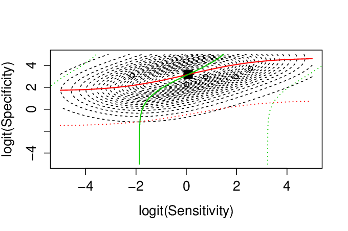 |
Comparing the results in Tables 5 and 6 for the surveillance of regional lymph node metastasis, US has the highest sensitivity (63%; 95% confidence interval CI = 50–77%) and specificity (95%; 95% CI = 93–97%). In contrast, patients diagnosed by PET have higher estimated prevalences of metastasis (37%; 95% confidence interval CI = 29–45%), compared with patients diagnosed by US (26%; 95% confidence interval CI = 12–40%).
Finally, in Table 7 we report the resulting maximized log-likelihoods, estimates, and standard errors of the hybrid copula mixed models with different choices of parametric families of copulas and margins for the for the PET modality to diagnose distant lymph node metastasis. All models roughly agree on the estimated sensitivity , specificity and disease prevalence for the surveillance of regional lymph node metastasis. The log-likelihoods show that a hybrid copula mixed model with Frank copulas and normal margins provides the best fit. It is also provides better inferences than a hybrid copula-based mixed model with independence among the random effects since the likelihood has been improved by units. This is also confirmed by a likelihood ratio test (-value ). Figure 3 shows the fitted SROC curves along with their confidence and prediction regions for the best fitted hybrid copula mixed model with normal margins for both case-control and cohort studies. In this dataset it revealed that there is heterogeneity in association between cohort and case control studies, i.e. is positive, while is negative.
| Normal margins | ||||||||||||||
| BVN | Frank | Cln180/270 | Cln 180/90 | Cln 0/270 | Cln 0/90 | CL | ||||||||
| Est. | SE | Est. | SE | Est. | SE | Est. | SE | Est. | SE | Est. | SE | Est. | SE | |
| 0.82 | 0.02 | 0.82 | 0.02 | 0.83 | 0.03 | 0.82 | 0.02 | 0.82 | 0.03 | 0.82 | 0.02 | 0.85 | 0.02 | |
| 0.87 | 0.02 | 0.87 | 0.02 | 0.87 | 0.03 | 0.87 | 0.02 | 0.87 | 0.03 | 0.87 | 0.02 | 0.88 | 0.02 | |
| 0.57 | 0.06 | 0.56 | 0.06 | 0.57 | 0.06 | 0.55 | 0.06 | 0.59 | 0.07 | 0.59 | 0.06 | 0.59 | 0.07 | |
| 0.65 | 0.16 | 0.65 | 0.16 | 0.65 | 0.17 | 0.64 | 0.15 | 0.68 | 0.17 | 0.65 | 0.15 | 0.64 | 0.09 | |
| 0.94 | 0.21 | 0.91 | 0.20 | 0.94 | 0.23 | 1.01 | 0.22 | 0.93 | 0.23 | 0.99 | 0.21 | 0.89 | 0.10 | |
| 0.87 | 0.20 | 0.93 | 0.21 | 0.94 | 0.21 | 0.92 | 0.21 | 0.89 | 0.22 | 0.84 | 0.19 | 0.97 | 0.18 | |
| -0.31 | 0.25 | -0.45 | 0.27 | -0.19 | 0.40 | -0.28 | 0.25 | -0.27 | 0.38 | -0.30 | 0.27 | 0.00 | - | |
| 0.52 | 0.20 | 0.51 | 0.21 | 0.51 | 0.21 | 0.46 | 0.21 | 0.53 | 0.22 | 0.49 | 0.22 | 0.00 | - | |
| 0.60 | 0.41 | 0.57 | 0.36 | 0.63 | 0.61 | 0.73 | 0.32 | 0.63 | 0.59 | 0.72 | 0.32 | 0.00 | - | |
| -174.50 | -174.46 | -175.98 | -175.03 | -174.93 | -173.93 | -178.80 | ||||||||
| Beta margins | ||||||||||||
| BVN | Frank | Cln 180/270 | Cln 180/90 | Cln 0/270 | Cln 0/90 | |||||||
| Est. | SE | Est. | SE | Est. | SE | Est. | SE | Est. | SE | Est. | SE | |
| 0.80 | 0.03 | 0.80 | 0.03 | 0.81 | 0.03 | 0.80 | 0.02 | 0.80 | 0.03 | 0.80 | 0.02 | |
| 0.84 | 0.03 | 0.83 | 0.03 | 0.84 | 0.03 | 0.84 | 0.03 | 0.83 | 0.03 | 0.84 | 0.03 | |
| 0.56 | 0.05 | 0.55 | 0.05 | 0.55 | 0.05 | 0.54 | 0.05 | 0.57 | 0.06 | 0.58 | 0.05 | |
| 0.06 | 0.03 | 0.06 | 0.03 | 0.06 | 0.03 | 0.05 | 0.02 | 0.06 | 0.03 | 0.06 | 0.03 | |
| 0.10 | 0.04 | 0.09 | 0.04 | 0.10 | 0.04 | 0.11 | 0.04 | 0.10 | 0.04 | 0.10 | 0.04 | |
| 0.14 | 0.05 | 0.15 | 0.05 | 0.16 | 0.05 | 0.15 | 0.05 | 0.15 | 0.06 | 0.13 | 0.05 | |
| -0.31 | 0.24 | -0.46 | 0.27 | -0.23 | 0.49 | -0.26 | 0.25 | -0.29 | 0.38 | -0.27 | 0.25 | |
| 0.53 | 0.20 | 0.53 | 0.21 | 0.51 | 0.21 | 0.47 | 0.21 | 0.55 | 0.22 | 0.50 | 0.22 | |
| 0.65 | 0.38 | 0.60 | 0.35 | 0.66 | 0.58 | 0.76 | 0.30 | 0.67 | 0.56 | 0.76 | 0.30 | |
| -175.76 | -175.69 | -177.17 | -176.37 | -176.14 | -175.33 | |||||||
Cln denotes a hybrid copula mixed with copula distributions the Clayton rotated by and degrees for the and copulas, respectively.
| Cohort studies | Case-Control studies |
|---|---|
 |
 |
In all the meta-analyses, improvement over the hybrid copula mixed model composed of BVN copulas and normal margins, that is the same with the hybrid GLMM in Chen et al., (2015), has been revealed in terms of the likelihood principle. Chen et al., (2015), instead of relying to separate meta-analyses for each type of imaging modality and type of metastasis, analyzed all the data by assuming normal margins for the random effects with equal between-studies variances in transformed sensitivity, specificity, and disease prevalence for different imaging modalities or stages of metastasis. These assumptions are quite strong and we have shown, with the subgroup analysis in Tables 5-7, that are substantially violated. In fact, between study variances are distinct in each type of imaging modality or stage of metastasis and for the US imaging modality even the assumption of normal margins is not valid.
6 Discussion
We have proposed a hybrid copula mixed model for meta-analysis of diagnostic test accuracy studies. It jointly models the disease prevalence along with diagnostic test sensitivity and specificity in cohort studies, and sensitivity and specificity in case-control studies. Our general model includes the hybrid GLMM (Chen et al.,, 2015) as a special case and can provide an improvement over the latter based on log-likelihood. Hence, a better statistical inference for the meta-analytic parameters and their between-study variances is achieved. Nevertheless the meta-analytic parameters are a univariate inference, and hence it is the univariate marginal distribution that matters the most and not the type of the copula. The proposed hybrid copula mixed model calls on both normal and beta univariate margins and thus can operate on the transformed and original scale of sensitivity, specificity and disease prevalence, respectively.
Though typically the focus of meta-analysis has been to derive the summary-effect estimates, there is increasing interest in drawing predictive inference. In fact, if the interest is only to overall sensitivity, specificity and prevalence then the overall test accuracy across studies will not be clearly defined. Different studies use different thresholds for a positive test result, thus the overall summary-effect estimates do not make sense. Instead, some form of SROC curve makes much more sense and will help decision makers to assess the actual diagnostic accuracy of a diagnostic test (Nikoloulopoulos, 2016a, ). SROC curves are deduced for our model through the quantile regression techniques developed by Nikoloulopoulos, 2015a (). For the hybrid copula mixed model, the model parameters (including dependence parameters), the choice of the copula, and the choice of the margin affect the shape of the SROC curve. Among the parametric families of copulas in Table 1 the tail dependence varies, and is a property to consider when choosing amongst different families of copulas, and, hence affects the shape of SROC curves, i.e., prediction. SROC will essentially show the effect of different model (random effect distribution) assumptions, since it is an inference that depends on the joint distribution (Nikoloulopoulos, 2015a, ). Given that the CL estimation assumes independence among the random effects, it provides identical fit for any copula mixed model, since all the parametric families of copulas in Table 1 contain the independence copula as a special case. Hence, the big limitation of the CL method is that it cannot be used to produce the SROC curves, since the dependence parameters affect the shape of the SROC curve and these are set to independence by definition.
It has been reported in the literature that in the trivariate GLMM (Chu et al.,, 2009) and hybrid GLMM (Chen et al.,, 2015) estimation problems relating to the correlation parameters exist, such as non-convergence. Here instead of a trivariate normal distribution we use a vine copula distribution, and in particular a truncated at level-1 vine copula (conditional independence), which allows both parsimony and flexible (tail) dependence. In fact, we propose a numerically stable ML estimation technique based on Gauss-Legendre quadrature; the crucial step is to convert from independent to dependent quadrature points. However, the additional feature of having to estimate the associations among the random effects has been found to require larger sample sizes than in CL estimation where these parameters are set to independence. The application example includes cases with an adequate number of individual studies per study design. For meta-analyses with fewer (especially cohort) studies the bivariate copula mixed model to obtain estimates of diagnostic sensitivity and specificity but not prevalence should be fitted instead. Future research will deal with the development of penalized likelihood methods for optimising inference about the association parameters of the hybrid copula mixed model when the number of available study summaries is small.
We also plan to provide extensions of the model to account for partial verification bias. This is a feature that has been already developed for the hybrid GLMM (Ma et al.,, 2014).
Software
R functions to implement the hybrid vine copula mixed model for meta-analysis of diagnostic test accuracy case-contol and cohort studies are part of the R package CopulaREMADA (Nikoloulopoulos, 2016b, ).
Acknowledgement
We would like to thank Dr Yong Chen (University of Texas) and Professor Haitao Chu (University of Minnesota) for providing the melanoma data.
References
- Aas et al., (2009) Aas, K., Czado, C., Frigessi, A., and Bakken, H. (2009). Pair-copula constructions of multiple dependence. Insurance: Mathematics & Economics, 44:182–198.
- Brenner and Gefeller, (1997) Brenner, H. and Gefeller, O. (1997). Variation of sensitivity, specificity, likelihood ratios and predictive values with disease prevalence. Statistics in Medicine, 16(9):981–991.
- Chen et al., (2015) Chen, Y., Liu, Y., Ning, J., Cormier, J., and Chu, H. (2015). A hybrid model for combining case–control and cohort studies in systematic reviews of diagnostic tests. Journal of the Royal Statistical Society: Series C (Applied Statistics), 64(3):469–489.
- Chen et al., (2014) Chen, Y., Liu, Y., Ning, J., Nie, L., Zhu, H., and Chu, H. (2014). A composite likelihood method for bivariate meta-analysis in diagnostic systematic reviews. Statistical Methods in Medical Research. DOI:10.1177/0962280214562146.
- Chu and Cole, (2006) Chu, H. and Cole, S. R. (2006). Bivariate meta-analysis of sensitivity and specificity with sparse data: a generalized linear mixed model approach. Journal of Clinical Epidemiology, 59(12):1331–1332.
- Chu et al., (2009) Chu, H., Nie, L., Cole, S. R., and Poole, C. (2009). Meta-analysis of diagnostic accuracy studies accounting for disease prevalence: Alternative parameterizations and model selection. Statistics in Medicine, 28(18):2384–2399.
- Demidenko, (2004) Demidenko, E. (2004). Mixed Models: Theory and Applications. John Wiley & Sons, Hoboken, New Jersey.
- Jerant et al., (2000) Jerant, A., Johnson, J., Sheridan, C., and Caffrey, T. (2000). Early detection and treatment of skin cancer. American Family Physician, 62(2):357–368+375–376+381–382.
- Joe, (1997) Joe, H. (1997). Multivariate Models and Dependence Concepts. Chapman & Hall, London.
- Joe, (2011) Joe, H. (2011). Dependence comparisons of vine copulae with four or more variables. In Kurowicka, D. and Joe, H., editors, Dependence Modeling: Handbook on Vine Copulae, chapter 7, pages 139–164. World Scientific, Singapore.
- Joe, (2014) Joe, H. (2014). Dependence Modeling with Copulas. Chapman & Hall, London.
- Joe et al., (2010) Joe, H., Li, H., and Nikoloulopoulos, A. K. (2010). Tail dependence functions and vine copulas. Journal of Multivariate Analysis, 101:252–270.
- Kurowicka and Joe, (2011) Kurowicka, D. and Joe, H. (2011). Dependence Modeling – Handbook on Vine Copulae. World Scientific Publishing Co, Singapore.
- Leeflang et al., (2013) Leeflang, M. M., Rutjes, A. W., Reitsma, J. B., Hooft, L., and Bossuyt, P. M. (2013). Variation of a test’s sensitivity and specificity with disease prevalence. Canadian Medical Association Journal, 185(11):E537–E544.
- Leeflang et al., (2009) Leeflang, M. M. G., Bossuyt, P. M. M., and Irwig, L. (2009). Diagnostic test accuracy may vary with prevalence: implications for evidence-based diagnosis. Journal of Clinical Epidemiology, 62(1):5–12.
- Ma et al., (2014) Ma, X., Chen, Y., Cole, S. R., and Chu, H. (2014). A hybrid bayesian hierarchical model combining cohort and case–control studies for meta-analysis of diagnostic tests: Accounting for partial verification bias. Statistical methods in medical research. DOI:10.1177/0962280214536703.
- Nash, (1990) Nash, J. (1990). Compact Numerical Methods for Computers: Linear Algebra and Function Minimisation. Hilger, New York. 2nd edition.
- Nelsen, (2006) Nelsen, R. B. (2006). An Introduction to Copulas. Springer-Verlag, New York.
- (19) Nikoloulopoulos, A. K. (2015a). A mixed effect model for bivariate meta-analysis of diagnostic test accuracy studies using a copula representation of the random effects distribution. Statistics in Medicine, 34:3842–3865.
- (20) Nikoloulopoulos, A. K. (2015b). A vine copula mixed effect model for trivariate meta-analysis of diagnostic test accuracy studies accounting for disease prevalence. Statistical Methods in Medical Research. DOI:10.1177/0962280215596769.
- (21) Nikoloulopoulos, A. K. (2016a). Comment on ‘A vine copula mixed effect model for trivariate meta-analysis of diagnostic test accuracy studies accounting for disease prevalence’. Statistical Methods in Medical Research, 25(2):988–991.
- (22) Nikoloulopoulos, A. K. (2016b). CopulaREMADA: Copula mixed effect models for bivariate and trivariate meta-analysis of diagnostic test accuracy studies. R package version 1.0.
- Nikoloulopoulos and Joe, (2015) Nikoloulopoulos, A. K. and Joe, H. (2015). Factor copula models for item response data. Psychometrika, 80:126–150.
- Nikoloulopoulos and Karlis, (2008) Nikoloulopoulos, A. K. and Karlis, D. (2008). Copula model evaluation based on parametric bootstrap. Computational Statistics & Data Analysis, 52:3342–3353.
- Sklar, (1959) Sklar, M. (1959). Fonctions de répartition à dimensions et leurs marges. Publications de l’Institut de Statistique de l’Université de Paris, 8:229–231.
- Stober et al., (2013) Stober, J., Joe, H., and Czado, C. (2013). Simplified pair copula constructions-limitations and extensions. Journal of Multivariate Analysis, 119:101–118.
- Stroud and Secrest, (1966) Stroud, A. H. and Secrest, D. (1966). Gaussian Quadrature Formulas. Prentice-Hall, Englewood Cliffs, NJ.
- Varin, (2008) Varin, C. (2008). On composite marginal likelihoods. Advances in Statistical Analysis, 92:1–28.
- Varin et al., (2011) Varin, C., Reid, N., and Firth, D. (2011). An overview of composite likelihood methods. Statistica Sinica, 21:5–42.
- Xing et al., (2011) Xing, Y., Bronstein, Y., Ross, M. I., Askew, R. L., Lee, J. E., Gershenwald, J. E., Royal, R., and Cormier, J. N. (2011). Contemporary diagnostic imaging modalities for the staging and surveillance of melanoma patients: a meta-analysis. Journal of the National Cancer Institute, 103(2):129–142.