On the Stability and Accuracy of Partially and Fully
Implicit Schemes for Phase Field Modeling

Journal: Elsevier

Jinchao Xu Email: xu@math.psu.edu Address: Department of Mathematics, Pennsylvania State University, University Park, PA, 16802, USA Corresponding author: Corresponding author Yukun Li Email: li.7907@osu.edu Address: Department of Mathematics, The Ohio State University, Columbus, OH, 43210, USA Shuonan Wu Email: sxw58@psu.edu Address: Department of Mathematics, Pennsylvania State University, University Park, PA, 16802, USA Arthur Bousquet Email: akb5670@psu.edu Address: Department of Mathematics, Pennsylvania State University, University Park, PA, 16802, USA

Abstract

We study in this paper the accuracy and stability of partially and fully implicit schemes for phase field modeling. Through theoretical and numerical analysis of Allen-Cahn and Cahn-Hillard models, we investigate the potential problems of using partially implicit schemes, demonstrate the importance of using fully implicit schemes and discuss the limitation of energy stability that are often used to evaluate the quality of a numerical scheme for phase-field modeling. In particular, we make the following observations:

1.

a convex splitting scheme (CSS in short) can be equivalent to some fully implicit scheme (FIS in short) with a much different time scaling and thus it may lack numerical accuracy;
2.

most implicit schemes (in discussions) are energy-stable if the time-step size is sufficiently small;
3.

a traditionally known conditionally energy-stable scheme still possess an unconditionally energy-stable physical solution;
4.

an unconditionally energy-stable scheme is not necessarily better than a conditionally energy-stable scheme when the time step size is not small enough;
5.

a first-order FIS for the Allen-Cahn model can be devised so that the maximum principle will be valid on the discrete level and hence the discrete phase variable satisfies $|u_{h}(x)|\leq 1$ for all $x$ and, furthermore, the linearized discretized system can be effectively preconditioned by discrete Poisson operators.

Keywords:

The Allen-Cahn model, the Cahn-Hilliard model, fully implicit schemes, convex splitting schemes, energy minimization.

1 Introduction

In this paper, we consider the following Allen-Cahn model [3]:

	$\displaystyle u_{t}-\Delta u+\frac{1}{\epsilon^{2}}f(u)$	$\displaystyle=0\qquad\mbox{in }\Omega_{T}:=\Omega\times(0,T),$		(1.1)
	$\displaystyle\frac{\partial u}{\partial n}$	$\displaystyle=0\qquad\mbox{on }\partial\Omega_{T}:=\partial\Omega\times(0,T),$		(1.1)

and the following Cahn-Hilliard model [7]:

$\displaystyle u_{t}-\Delta w$	$\displaystyle=0\qquad\mbox{in }\Omega_{T},$	(1.2)
$\displaystyle-\epsilon\Delta u+\frac{1}{\epsilon}f(u)$	$\displaystyle=w\qquad\mbox{in }\Omega_{T},$
$\displaystyle\frac{\partial u}{\partial n}=\frac{\partial w}{\partial n}$	$\displaystyle=0\qquad\mbox{on }\partial\Omega_{T}.$

The initial condition is set as $u|_{t=0}=u_{0}$ . Here, $T$ is the end time, $\Omega\subset\mathbb{R}^{d}\,(d=2,3)$ is a bounded domain and $f=F^{\prime}$ for some double well potential $F$ which, in this paper, is taken to be the following polynomial:

F(u)=\frac{1}{4}(u^{2}-1)^{2}.

(1.3)

In recent years, there have been a lot of studies in the literature on the modeling aspects and their numerical solutions for both Allen-Cahn and Cahn-Hilliard equations. For the modeling aspects, we refer to [3, 6, 7, 35, 9, 10, 16, 4, 45]. In this paper, we will focus on the numerical schemes for both these equations. Among the various different schemes studied in the literature, a special class of partially implicit schemes, known as convex splitting schemes, appears to be most popular, c.f. [27, 26, 22, 38, 40, 47, 19] for the Allen-Cahn equation and [27, 1, 22, 40, 38, 41, 26, 20, 17] for the Cahn-Hilliard model. The popularity of the CSS is due to, among others, its two advantages: (1) a typical CSS is unconditionally energy-stable without any stringent restriction pertaining to the time step; (2) the resulting nonlinear numerical system can be easily solved (e.g. Newton iteration is guaranteed to converge regardless of the initial guess). In comparison, a standard fully implicit scheme is only energy-stable when the time step size is sufficiently small.

It is against the conventional wisdom that a partially implicit scheme such as the convex splitting scheme has a better stability property than a fully implicit scheme. One main goal of this paper is to understand this unusual phenomenon. For the Allen-Cahn model, we prove that the standard first-order CSS is exactly the same as the standard first-order FIS but with a (much) smaller time step size and as a result, it would provide an approximation to the original solution of the Allen-Cahn model at a delayed time (although the magnitude of the delay is reduced when the time step size is reduced). Such a time delay is also observed for other partially implicit schemes when time step size is not sufficient small. For the Cahn-Hilliard model, we prove that the standard CSS is exactly the same as the standard FIS for a different model that is a (nontrivial) perturbation of the original Cahn-Hilliard model. This at least explains theoretically why a CSS has a better stability property than a FIS does since a CSS is actually a FIS with a very small time-step size. In addition, we argue that such a gain of stability is at the expense of a possible loss of accuracy.

Given the aforementioned equivalences between CSS and FIS and the popularity of CSS in the literature, the value of FIS with a seemingly stringent time-step constraint (which, again, are equivalent to CSS without any time-step constraint) should be re-examined. Indeed, the importance of using fully implicit schemes for the phase field simulations has been addressed in the existing literature, e.g. [15, 21, 18, 37, 24, 38, 25, 27, 19, 20, 31, 45]. In this paper, we further study three families of new algorithms for FIS. First, we revisit the standard fully implicit scheme by extending it to a energy minimization problem at each time step. The minimization problem, however, admits a non-convex discrete energy when the time step size is not sufficiently small. Furthermore, we will be able to prove, rather straightforwardly, that the global minimizer satisfies the unconditional energy-stability, which is a natural property for linear systems and the desired property for the nonlinear systems like the Allen-Cahn or the Cahn-Hilliard equations. The results given by the energy minimization problem is quite different from those given by the standard fully implicit scheme. More precisely, instead of the severe restriction pertaining to the time step size, the energy minimization problem gives a good approximation to the physical solution only when the discretization error in time is controlled. Moreover, with the energy minimization problem, various minimization solvers (e.g. L-BFGS [32, 5]) can be efficiently applied. This may lead a promising direction to the design of accurate and efficient numerical schemes for phase field modeling.

Secondly, we propose a modification of a typical FIS for the Allen-Cahn so that the maximum principle will be valid on the discrete level. Thirdly, for this modified FIS scheme, we rigorously show that, under the appropriate time-step size constraint, the linearization of such a modified FIS can be uniformly preconditioned by a Poisson-like operator.

Second-order partially implicit schemes have also been designed in the literature with the same purpose of allowing large time step size as the first-order partially implicit schemes. But similar to the standard CSS, the time delay happens with large time step size. Actually, the second-order CSS (cf. [27, 38, 40, 47]) can also be viewed as the modified Crank-Nicolson scheme [15, 40, 13] on the artificially convexified model. Further, we demonstrate that, through numerical experiments with the modified Crank-Nicolson scheme, an unconditionally energy stable scheme is not necessarily better than a conditionally energy stable scheme.

The rest of paper is organized as follows. In §2, we focus on the first-order schemes. We study the convexity of the fully implicit scheme, prove that a typical first-order CSS is exactly equivalent to some first-order FIS. We also introduce the energy minimization version of some first-order FIS, and show that the convex splitting schemes can be viewed as artificial convexity schemes. In §3, we propose a modified FIS (or CSS) that satisfies maximum principle on the discrete level and further prove that the modified scheme can be preconditioned by a Poisson-like operator. In §4, we discuss the second-order schemes. We study a modified Crank-Nicolson scheme and its convex splitting version, compare the modified Crank-Nicolson scheme and some other second-order partially implicit schemes. Finally, in §5, we give some concluding remarks.

2 First-order schemes

First, we introduce some notation. Let $\mathcal{T}_{h}$ be a shape-regular (which may not be quasi-uniform) triangulation of $\Omega\subset\mathbb{R}^{d}\ (d=2,3)$ . The nodes of $\mathcal{T}_{h}$ is denoted by $\mathcal{N}_{h}$ . $K$ represents each element and $\overline{\Omega}=\bigcup_{K\in\mathcal{T}_{h}}\overline{K}$ . Let $h_{K}$ denote the diameter of $K\in\mathcal{T}_{h}$ and $h:=\mbox{max}\{h_{K};K\in\mathcal{T}_{h}\}$ . Define the finite element space $V_{h}$ by

V_{h}=\bigl\{v_{h}\in C(\overline{\Omega}):v_{h}|_{K}=P_{r}(K)\bigr\},

(2.1)

where $P_{r}(K)$ denotes the set of all polynomials whose degrees do not exceed a given positive integer $r$ on $K$ . The $L^{2}$ -inner product over the domain $\Omega$ is denoted by $(\cdot,\cdot)$ . For the time discretization, let $k_{n}$ denote the time step size on $n$ -th step and $t_{n}:=\sum_{i=1}^{n}k_{i}$ .

2.1 Fully implicit schemes and their convexity and energy stability properties

A standard first-order fully implicit scheme to problem (1.1) (FIS in short) is defined by seeking $u_{h}^{n}\in V_{h}$ for $n=1,2,\cdots$ , such that

(\frac{u_{h}^{n}-u_{h}^{n-1}}{k_{n}},v_{h})+(\nabla u_{h}^{n},\nabla v_{h})+\frac{1}{\epsilon^{2}}(f(u_{h}^{n}),v_{h})=0\qquad\forall v_{h}\in V_{h}.

(2.2)

A standard first-order FIS to problem (1.2) is defined by seeking $u_{h}^{n}\in V_{h}$ and $w_{h}^{n}\in V_{h}$ for $n=1,2,\cdots$ , such that

	$\displaystyle(\frac{u_{h}^{n}-u_{h}^{n-1}}{k_{n}},\eta_{h})+(\nabla w_{h}^{n},\nabla\eta_{h})$	$\displaystyle=0\qquad\forall\,\eta_{h}\in V_{h},$		(2.3)
	$\displaystyle\epsilon(\nabla u_{h}^{n},\nabla v_{h})+\frac{1}{\epsilon}((u_{h}^{n})^{3}-u_{h}^{n},v_{h})-(w_{h}^{n},v_{h})$	$\displaystyle=0\qquad\forall\,v_{h}\in V_{h}.$		(2.3)

Following [16, 29], the Allen-Cahn equation (1.1) can be interpreted as the $L^{2}$ -gradient flow for the free-energy functional, namely

	$\displaystyle J_{\epsilon}^{\rm AC}(v)$	$\displaystyle:=\int_{\Omega}\Bigl(\frac{1}{2}\|\nabla v\|^{2}+\frac{1}{\epsilon^{2}}F(v)\Bigr)\,dx,$		(2.4)
	$\displaystyle\frac{d}{dt}J_{\epsilon}^{\rm AC}(u(t))$	$\displaystyle=\bigl(-\Delta u+\frac{1}{\epsilon^{2}}f(u),u_{t}\bigr)_{L^{2}(\Omega)}=-\\|u_{t}\\|_{L^{2}(\Omega)}^{2}\leq 0.$		(2.4)

Following [2, 10, 36], the Cahn-Hilliard equations (1.2) can be interpreted as the $H^{-1}$ -gradient flow for the free-energy functional, namely

	$\displaystyle J_{\epsilon}^{\rm CH}(v)$	$\displaystyle:=\int_{\Omega}\Bigl(\frac{\epsilon}{2}\|\nabla v\|^{2}+\frac{1}{\epsilon}F(v)\Bigr)\,dx,$		(2.5)
	$\displaystyle\frac{d}{dt}J_{\epsilon}^{\rm CH}(u(t))$	$\displaystyle=\bigl(\Delta(\epsilon\Delta u-\frac{1}{\epsilon}f(u)),u_{t}\bigr)_{H^{-1}(\Omega)}=-\\|u_{t}\\|_{H^{-1}(\Omega)}^{2}\leq 0.$		(2.5)

Therefore, we say that a discretization scheme such as (2.2) or (2.3) is energy-stable if

J_{\epsilon}^{\rm AC}(u^{n}_{h})\leq J_{\epsilon}^{\rm AC}(u^{n-1}_{h})\quad\mbox{or}\quad J_{\epsilon}^{\rm CH}(u^{n}_{h})\leq J_{\epsilon}^{\rm CH}(u^{n-1}_{h})\qquad n=1,2,\ldots

(2.6)

We would like to point out that the concept of energy-stability for the nonlinear schemes such as (2.2) or (2.3) is different from the standard concept of stability for linear schemes. For most linear systems (e.g. heat equation), a fully implicit scheme is usually unconditionally stable. But for nonlinear systems, fully implicit schemes such as (2.2) or (2.3) are only conditionally energy-stable, namely they are only energy-stable when the time-step size $k_{n}$ is appropriately small. This is well-known fact in the phase-field literature (cf. [21, 25]). For completeness, we will study this energy-stability property through the study of the convexity of the relevant schemes. Further, we extend the standard schemes to the energy minimization versions at each time step, which seem to have better numerically performance.

2.1.1 Convexity of fully implicit schemes for the Allen-Cahn equation

In this section, we next study the convexity property of the FIS of the Allen-Cahn and Cahn-Hilliard equations. Consider the Allen-Cahn equation, in view of (2.4), we define the following discrete energy

E_{n}^{\rm AC}(u_{h};u_{h}^{n-1})=J_{\epsilon}^{\rm AC}(u_{h})+\frac{1}{2k_{n}}\int_{\Omega}(u_{h}-u_{h}^{n-1})^{2}dx.

(2.7)

We also extend the standard first-order fully implicit scheme to the following energy minimization problem:

u_{h}^{n}=\underset{u_{h}\in V_{h}}{\mathrm{argmin}}E_{n}^{\rm AC}(u_{h};u_{h}^{n-1}).

(2.8)

Theorem 2.1.

We have

1.

Under the condition that $k_{n}\leq\epsilon^{2}$ , $E_{n}^{\rm AC}(\cdot;u_{h}^{n-1})$ is strictly convex on $V_{h}$ .
2.

The solution of (2.2) satisfies $(E_{n}^{\rm AC})^{\prime}(u_{h}^{n};u_{h}^{n-1})(v_{h})=0$ .

The following discrete energy law holds for (2.8)

\displaystyle J_{\epsilon}^{\rm AC}(u_{h}^{n})+\frac{1}{2k_{n}}\|u_{h}^{n}-u_{h}^{n-1}\|_{L^{2}(\Omega)}^{2}\leq J_{\epsilon}^{\rm AC}(u_{h}^{n-1}).

(2.9)

Proof.

Taking the second derivative of $E_{n}^{\rm AC}(\cdot;u_{h}^{n-1})$ , we get for any $v_{h}\in V_{h}$ ,

(E_{n}^{\rm AC})^{\prime\prime}(u_{h};u_{h}^{n-1})(v_{h},v_{h})=\frac{3}{\epsilon^{2}}\int_{\Omega}u_{h}^{2}v_{h}^{2}dx+\int_{\Omega}(\frac{1}{k_{n}}-\frac{1}{\epsilon^{2}})v_{h}^{2}dx+\|\nabla v_{h}\|_{L^{2}(\Omega)}^{2}.

(2.10)

When $k_{n}\leq\epsilon^{2}$ , $(E_{n}^{\rm AC})^{\prime\prime}(u_{h};u_{h}^{n-1})(v_{h},v_{h})>0$ when $v_{h}\neq 0$ , which means $E(\cdot;u_{h}^{n-1})$ is strictly convex on $V_{h}$ . A direct calculation shows that (2.2) satisfies $(E_{n}^{\rm AC})^{\prime}(u_{h}^{n};u_{h}^{n-1})(v_{h})=0$ , and the following coercivity condition holds:

E_{n}^{\rm AC}(u_{h};u_{h}^{n-1})\geq M_{1}\|u_{h}\|_{H^{1}(\Omega)}^{2}-M_{2},

(2.11)

where $M_{1}$ and $M_{2}$ are positive constants that depend on $\epsilon$ . Then the unique solvability of (2.2) follows from [12] and (2.11). Moreover, for the global minimizer of (2.8), we have

J_{\epsilon}^{\rm AC}(u_{h}^{n})+\frac{1}{2k_{n}}\|u_{h}^{n}-u_{h}^{n-1}\|_{L^{2}(\Omega)}^{2}=E_{n}^{\rm AC}(u_{h}^{n};u_{h}^{n-1})\leq E_{n}^{\rm AC}(u_{h}^{n-1};u_{h}^{n-1})=J_{\epsilon}^{\rm AC}(u_{h}^{n-1}).

Then we finish the proof. ∎

In view of Theorem 2.1, let us introduce the terminology of convex scheme. We say that a scheme is convex if it is equivalent to the minimization of a convex functional. Thus (2.2) is a convex scheme under the condition $k_{n}\leq\epsilon^{2}$ , under which the first-order FIS (2.2) is equivalent to the energy minimization version (2.8). When $k_{n}>\epsilon^{2}$ , the $E_{n}^{\rm AC}(\cdot;u_{h}^{n-1})$ may not be convex, hence the standard Newton’s method for (2.2) may fail in this case. Thus, generally speaking, the scheme (2.8) calls for the global minimization solver.

2.1.2 Convexity of fully implicit scheme for the Cahn-Hilliard equation

Define the discrete Laplace operator $\Delta_{h}:{V}_{h}\mapsto{V}_{h}$ as follows: Given $v_{h}\in{V}_{h}$ , let $\Delta_{h}v_{h}\in{V}_{h}$ such that

(\Delta_{h}v_{h},w_{h})=-(\nabla v_{h},\nabla w_{h})\qquad\forall\,w_{h}\in V_{h}.

(2.12)

Let $L^{2}_{0}$ denote the collection of functions in $L^{2}(\Omega)$ with zero mean, and let $\mathring{V}_{h}:=V_{h}\cap L^{2}_{0}$ . Taking $w_{h}=1$ in (2.12), we know that $\text{Range}(\Delta_{h})\subset\mathring{V}_{h}$ . Further, the well-posedness of the Poisson problem with Neumann boundary condition on $\mathring{V}_{h}$ implies that $\text{Range}(\Delta_{h})=\mathring{V}_{h}$ . Therefore, $\Delta_{h}|_{\mathring{V}_{h}}:\mathring{V}_{h}\mapsto\mathring{V}_{h}$ is an isomorphism, then $\Delta_{h}^{-1}:=(\Delta_{h}|_{\mathring{V}_{h}})^{-1}:\mathring{V}_{h}\mapsto\mathring{V}_{h}$ is well-defined.

Consider the Cahn-Hilliard equations, in view of (2.5), we define the discrete energy

E_{n}^{\rm CH}(\theta_{h};u_{h}^{n-1})=J_{\epsilon}^{\rm CH}(u_{h}^{n-1}+\theta_{h})+\frac{1}{2k_{n}}\|\nabla\Delta_{h}^{-1}\theta_{h}\|_{L^{2}(\Omega)}^{2}\qquad\theta_{h}\in\mathring{V}_{h}.

(2.13)

Then, the energy minimization version of the first-order FIS for the Cahn-Hilliard equations is shown to be

\theta_{h}^{n}=\underset{\theta_{h}\in\mathring{V}_{h}}{\mathrm{argmin}}E_{n}^{\rm CH}(\theta_{h};u_{h}^{n-1}),\qquad u_{h}^{n}=u_{h}^{n-1}+\theta_{h}^{n}.

(2.14)

Theorem 2.2.

We have

1.

Under the condition that $k\leq 4\epsilon^{3}$ , $E_{n}^{\rm CH}(\cdot;u_{h}^{n-1})$ is convex on $\mathring{V}_{h}$ .
2.

The solution of (2.3) satisfies $u_{h}^{n}=u_{h}^{n-1}+\theta_{h}$ , with $(E_{n}^{\rm CH})^{\prime}(\theta_{h};u_{h}^{n-1})(v_{h})=0$ .

The following energy law holds for (2.14)

J_{\epsilon}^{\rm CH}(u_{h}^{n})+\frac{1}{2k_{n}}\|\nabla\Delta_{h}^{-1}(u_{h}^{n}-u_{h}^{n-1})\|_{L^{2}(\Omega)}^{2}\leq J_{\epsilon}^{\rm CH}(u_{h}^{n-1}).

(2.15)

Proof.

For any $\theta_{h},\eta_{h}\in\mathring{V}_{h}$ , we have

(E_{n}^{\rm CH})^{\prime\prime}(\theta_{h};u_{h}^{n-1})(\eta_{h},\eta_{h})=\frac{1}{{\epsilon}}\int_{\Omega}\bigl(3(u_{h}^{n-1}+\theta_{h})^{2}-1\bigr)\eta_{h}^{2}~dx+\frac{1}{k_{n}}\|\nabla\Delta_{h}^{-1}\eta_{h}\|_{L^{2}(\Omega)}^{2}+\epsilon\|\nabla\eta_{h}\|_{L^{2}(\Omega)}^{2}.

Using Schwarz’s inequality, we have

\frac{1}{\epsilon}\|\eta_{h}\|_{L^{2}(\Omega)}^{2}\leq\frac{1}{\epsilon}(\Delta_{h}^{-1}\eta_{h},\eta_{h})^{1/2}(\Delta_{h}\eta_{h},\eta_{h})^{1/2}\leq\frac{1}{4\epsilon^{3}}\|\nabla\Delta_{h}^{-1}\eta_{h}\|_{L^{2}(\Omega)}^{2}+\epsilon\|\nabla\eta_{h}\|_{L^{2}(\Omega)}^{2}.

When $k_{n}\leq 4\epsilon^{3}$ ,

\displaystyle(E_{n}^{\rm CH})^{\prime\prime}(\theta_{h};u_{h}^{n-1})(\eta_{h},\eta_{h})\geq\frac{1}{{\epsilon}}\int_{\Omega}3(u_{h}^{n-1}+\theta_{h})^{2}\eta_{h}^{2}~dx+(\frac{1}{k_{n}}-\frac{1}{4\epsilon^{3}})\|\nabla\Delta_{h}^{-1}\eta_{h}\|_{L^{2}(\Omega)}^{2}\geq 0,

(2.16)

where the strict inequality holds when $\eta_{h}\neq 0$ . This means that $(E_{n}^{\rm CH})(\cdot;u_{h}^{n-1})$ is strictly convex on $\mathring{V}_{h}$ .

Now, taking $\eta_{h}=1$ in (2.3), we have $u_{h}^{n}\in u_{h}^{n-1}+\mathring{V}_{h}$ . Let $v_{h}=1$ in (2.3), we have $\int_{\Omega}w_{h}^{n}dx=\frac{1}{\epsilon}\int_{\Omega}f(u_{h}^{n})dx$ . Then, the first equation of (2.3) is equivalent to

w_{h}^{n}=\frac{1}{k_{n}}\Delta_{h}^{-1}(u_{h}^{n}-u_{h}^{n-1})+\frac{1}{\epsilon|\Omega|}\int_{\Omega}f(u_{h}^{n})dx.

Therefore, (2.3) is shown to be

\epsilon(\nabla u_{h}^{n},\nabla v_{h})+\frac{1}{\epsilon}((I-Q_{0})f(u_{h}^{n}),v_{h})-\frac{1}{k_{n}}(\Delta_{h}^{-1}(u_{h}^{n}-u_{h}^{n-1}),v_{h})=0\qquad\forall~v_{h}\in V_{h}.

(2.17)

where $Q_{0}:L^{2}(\Omega)\mapsto\mathbb{R}$ is the $L^{2}$ projection, namely $Q_{0}v=\frac{1}{|\Omega|}\int_{\Omega}vdx$ . Let $\theta_{h}=u_{h}^{n}-u_{h}^{n-1}\in\mathring{V}_{h}$ . Note that $Q_{0}\theta_{h}=Q_{0}\Delta^{-1}\theta_{h}=0$ , we can then write (2.17) as

\epsilon(\nabla(u_{h}^{n-1}+\theta_{h}),\nabla(I-Q_{0})v_{h})+\frac{1}{\epsilon}(f(u_{h}^{n-1}+\theta_{h}),(I-Q_{0})v_{h})-\frac{1}{k_{n}}(\Delta_{h}^{-1}\theta_{h},(I-Q_{0})v_{h})=0\quad\forall~v_{h}\in V_{h}.

This means that

\epsilon(\nabla(u_{h}^{n-1}+\theta_{h}),\nabla v_{h})+\frac{1}{\epsilon}(f(u_{h}^{n-1}+\theta_{h}),v_{h})-\frac{1}{k_{n}}(\Delta_{h}^{-1}\theta_{h},v_{h})=0\qquad\forall~v_{h}\in\mathring{V}_{h},

which can be recast as $(E_{n}^{\rm CH})^{\prime}(\theta_{h};u_{h}^{n-1})(v_{h})=0$ . The unique solvability and energy stability (2.15) then follows from the similar argument in Theorem 2.1. ∎

2.2 Convex splitting schemes and their equivalence to fully implicit schemes

As we have seen before, convexity is a very desirable property of the discretize scheme and fully implicit scheme is only convex when $k$ is sufficiently small. When $k$ is not sufficiently small, the non-convexity of the discrete scheme comes from the fact that the potential function $F$ in (1.3) is not convex. The convex splitting scheme (CSS in short) stems from splitting the non-convex potential function $F$ given by (1.3) into the difference between two convex functions:

F(u)=F_{+}(u)-F_{-}(u),\quad\mbox{with}\quad F_{+}(u)=\frac{1}{4}(u^{4}+1),\quad F_{-}(u)=\frac{1}{2}u^{2}.

(2.18)

2.2.1 A convex splitting scheme for the Allen-Cahn model

In view of Theorem 2.1, a CSS be obtained by making the non-convex part, namely $-F_{-}(\cdot)$ in (2.18), explicit in some way, and it can be characterized by the minimization of a convex functional:

u_{h}^{n}=\underset{u_{h}\in V_{h}}{\mathrm{argmin}}\bigg\{\int_{\Omega}\Bigl(\frac{1}{2}|\nabla u_{h}|^{2}+\frac{1}{\epsilon^{2}}[F_{+}(u_{h})-\hat{F}_{-}(u_{h};u_{h}^{n-1})]\Bigr)\,dx+\frac{1}{2k_{n}}\int_{\Omega}(u_{h}-u_{h}^{n-1})^{2}dx\bigg\},

(2.19)

where $\hat{F}_{-}(u_{h};u_{h}^{n-1})$ is the linearization of $F_{-}(\cdot)$ at $u_{h}^{n-1}$ , that is, $\hat{F}_{-}(u_{h};u_{h}^{n-1})=F_{-}(u_{h}^{n-1})+F_{-}^{\prime}(u_{h}^{n-1})(u_{h}-u_{h}^{n-1})$ .

The variational formulation of (2.19) is the following well-known CSS: Find $u_{h}^{n}\in V_{h}$ for $n=1,2,\cdots$ , such that

(\frac{u_{h}^{n}-u_{h}^{n-1}}{k_{n}},v_{h})+(\nabla u_{h}^{n},\nabla v_{h})+\frac{1}{\epsilon^{2}}((u_{h}^{n})^{3}-u_{h}^{n-1},v_{h})=0\qquad\forall v_{h}\in V_{h}.

(2.20)

Theorem 2.3.

[17] The CSS scheme (2.20) is unconditionally energy stable.

At the first glance, the above result looks incredibly remarkable. As we have seen above, even a fully implicit scheme can not be unconditionally energy-stable, but as a partially implicit (or explicit) scheme, CSS is unconditionally energy-stable. Although, as we discussed before, we can not quite relate the energy-stability in a nonlinear scheme to the standard stability concept in a standard linear scheme, it is quite incredible that a partially implicit (or explicit) scheme is actually more stable than a fully implicit scheme!

This remarkable phenomenon can be explained by the following result.

Theorem 2.4.

The CSS (2.20) can be recast as the FIS (2.2) with different time step size:

k_{n}^{\prime}=\frac{\epsilon^{2}}{k_{n}+\epsilon^{2}}k_{n}.

(2.21)

Proof.

We write that

(u_{h}^{n})^{3}-u_{h}^{n-1}=f(u_{h}^{n})+(u_{h}^{n}-u_{h}^{n-1}).

Substituting the above identity into (2.20) and regrouping the term involving $u_{h}^{n}-u_{h}^{n-1}$ , we obtain

\displaystyle\bigl((\frac{1}{k_{n}}+\frac{1}{\epsilon^{2}})(u_{h}^{n}-u_{h}^{n-1}),v_{h}\bigr)+(\nabla u_{h}^{n},\nabla v_{h})+\frac{1}{\epsilon^{2}}(f(u_{h}^{n}),v_{h})=0\qquad\forall v_{h}\in V_{h},

(2.22)

which is exactly the FIS with time step size (2.21). ∎

By comparing the condition for the time step size in Theorem 2.1 and (2.21), the resulting time-step constraint (2.21) in the CSS is actually more stringent to assure the convexity of the original FIS, as $k_{n}^{\prime}<\epsilon^{2}$ for any $\epsilon>0$ . This also explains why the CSS is always energy-stable thanks to the Theorem 2.1.

Remark 2.1.

We now make some remark on the implication of Theorem 2.4. Let $u_{h}^{\rm FIS}(t_{n})$ be the solution to (2.2) and $u_{h}^{{\rm CSS}}(t_{n})$ be the solution to (2.20). Then by Theorem 2.4, we have

u_{h}^{{\rm CSS}}(t_{n})=u_{h}^{{\rm FIS}}(\delta_{n}t_{n}),\quad\mbox{with}\quad\delta_{n}=\frac{\epsilon^{2}}{k_{n}+\epsilon^{2}}.

(2.23)

Here, $\delta_{n}$ can be regarded as a delaying factor. A larger time step size $k_{n}$ , which gives a smaller $\delta_{n}$ , leads to a more significant time-delay. Even for a very small $k_{n}$ , such a delay is not negligible. For example, if $k_{n}=\epsilon^{2}$ , we have $\delta_{n}=1/2$ . Thus, $u_{h}^{{\rm CSS}}(t_{n})=u_{h}^{{\rm FIS}}(\frac{t_{n}}{2})$ .

Because of such a delay, it is expected and also numerically verified that, quantitatively speaking, the CSS may have a reduced accuracy although it gives qualitatively correct answer. Furthermore such a delay will diminish as $k_{n}\to 0$ since $\lim_{k_{n}\to 0}\delta_{n}=1$ .

In summary, we conclude that the CSS has a special property that may be known as “delayed convergence” in the following sense:

1.

The CSS scheme is expected to eventually converge to the exact solution of the originally Allen-Cahn equation as $k_{n}\to 0$ .
2.

But for any given time step size $k_{n}$ , the CSS would approximate better the exact solution at a delayed time.

Test 1

In this test, the square domain $\Omega=(-1,1)^{2}$ is used to investigate the performance of different numerical schemes, and the initial condition is chosen as

\displaystyle u_{0}=\tanh\bigl(\frac{d_{0}(x)}{\sqrt{2}\epsilon}\bigr).

(2.24)

Here, $d_{0}(x)$ is the signed distance function from $x$ to the initial curve $\Gamma_{0}:x^{2}+y^{2}=0.6^{2}$ , i.e., $d_{0}(x)=\sqrt{x^{2}+y^{2}}-0.6$ . Figure 2.1 and 2.2 displays the evolution of the radius with respect to time. The singularity happens at $t=0.18$ , which is the disappearing time.

The numerical solutions of FIS and CSS with different $h$ ’s are plotted in Figure 2.1. When decreasing $h$ , the FIS approximates the exact solution well, while the CSS does not. The similar phenomenon happens with different $\epsilon$ ’s, as shown in Figure 2.2.

Test 2

In this simulation, we minimize the discrete energy (2.7) for the Allen-Cahn equation at each time step. The computational domain is $\Omega=(-1,1)^{2}$ , and parameter is $\epsilon=5\times 10^{-3}$ . The initial value, shown in Figure 2.3a, is chosen as

u_{0}(x,y)=\tanh\left(\frac{\sqrt{x^{2}+y^{2}}-0.6}{\sqrt{2}\epsilon}\right).

(2.25)

When $t$ increases, we expect the radius of the hole to decrease, as shown in Figure 2.3b.

Our goal is to test if the solution from the energy minimization scheme approximates the physical solution even when the discrete energy is non-convex. Recall that when $k_{n}\leq\epsilon^{2}$ , the discrete energy is convex.

We first test the dependency on the initial guess for the L-BFGS minimization algorithm (cf. [32, 5]). Here we choose $k_{1}=10^{-3}$ , which leads to the non-convex discrete energy (2.4). Figure 2.4a shows the global minimizer by using $u_{0}(x,y)$ as the initial guess for the L-BFGS, which is quite similar to the solution obtained with $k_{n}=10^{-5}$ , see Figure 2.5; Figure 2.4b shows a local minimizer by using the initial guess for L-BFGS as $1-u_{0}(x,y)$ . We observe that when the initial guess is the solution at previous time step, the local minimizer has lowest discrete energy, and that the solution with the lowest discrete energy is the best approximation to the solution obtained in the convex case.

We compare the solution for $k_{n}=10^{-5}$ , for the case in which the discrete energy is convex, with the solutions for $k_{n}=10^{-4}$ and $k_{n}=10^{-3}$ , for the cases in which the discrete energies are non-convex. For the L-BFGS algorithm, the initial guess is set to be the solution at previous time step. Figure 2.5 displays the cross-sectional solutions at $y=0$ at different $t$ ’s. We observe that energy minimization version of fully implicit schemes performs all well with different time step sizes.

Since the initial guess for the L-BFGS algorithm is random, we conclude that the L-BFGS algorithm does not depend on the initial guess when the solution is smooth enough. We also compare the evolutions of physical energies $J_{\epsilon}^{\rm AC}$ for the three cases in Figure 2.6, which shows that the energy minimization version of fully implicit scheme is energy-stable.

Test 3

In this set of simulations, we minimize the discrete energy (2.7) for the Allen-Cahn equation with $\epsilon=5\times 10^{-3}$ at each time step. The computational domain is chosen as $\Omega=(-1,1)^{2}$ , while the initial value $u_{0}(x,y)$ is randomly chosen.

In order to smooth the initial value, we first compute the solution from $t=0$ to $t=2\times 10^{-3}$ with $k=10^{-5}$ , namely

k_{n}=10^{-5}\qquad\text{for }n=1,2,\cdots,200.

Then, we switch for different time step sizes with the energy minimization version of fully implicit scheme. This is needed only when $k_{n}\geq 10^{-3}$ .

After the smoothing the random initial value, we first test the dependency on the initial guess for the L-BFGS minimization algorithm. Here we choose $k_{201}=10^{-3}$ , which leads to the non-convex discrete energy (2.7). The reference solution is obtained by evolving the Allen-Cahn equation with $k_{n}=10^{-5}$ (convex case). Figure 2.7 shows the different local minimizers from different initial guesses. We observe that: (1) When the initial guess is the solution at previous time step, the local minimizer has lowest discrete energy; (2) The solution with the lowest discrete energy is the best approximation to the reference solution; (3) When the initial guesses are random chosen, we obtain several different local minimizers. This implies that the result obtained from L-BFGS does depend on the initial guess when the solution is not smooth enough. Therefore, we will (and recommend to) choose the solution at previous time step as the initial guess for the L-BFGS algorithm.

Next, we evolve the Allen-Cahn equation with different time step sizes after $t=2\times 10^{-3}$ to see the two phases regroup. Three different computations with $k_{n}=10^{-5}$ (convex case), $k_{n}=10^{-4}$ and $k_{n}=10^{-3}$ (non-convex cases) are considered. In Figure 2.8 shows the random initial value and the evolutions of the numerical solutions at different $t$ ’s. It can be observed that the solutions in all these cases behave similarly. In addition, for the given random initial condition, the evolution of physical solution and physical energy seem a little bit faster than the others when choosing $k_{n}=10^{-3}$ , as shown in Figure 2.9. This is most likely because of the time discretization error for the large time step size. Furthermore, the evolutions of the physical energies show the energy-stability of the energy minimization version of the fully implicit scheme, which is in agreement with the Theorem 2.1.

2.2.2 A convex splitting scheme for the Cahn-Hilliard model

Similar to the Allen-Cahn model, a convex splitting scheme can also be obtained for Cahn-Hilliard model as follows: Find $u_{h}^{n}\in V_{h}$ for $n=1,2,\cdots,N$ , such that

	$\displaystyle(\frac{u_{h}^{n}-u_{h}^{n-1}}{k_{n}},\eta_{h})+(\nabla w_{h}^{n},\nabla\eta_{h})$	$\displaystyle=0\qquad\forall\,\eta_{h}\in V_{h},$		(2.26)
	$\displaystyle\epsilon(\nabla u_{h}^{n},\nabla v_{h})+\frac{1}{\epsilon}((u_{h}^{n})^{3}-u_{h}^{n-1},v_{h})-(w_{h}^{n},v_{h})$	$\displaystyle=0\qquad\forall\,v_{h}\in V_{h}.$		(2.26)

Theorem 2.5.

The Discretization of the Cahn-Hilliard equation using the convex splitting scheme is equivalent to the discretization of the following equations using the fully implicit scheme:

	$\displaystyle u_{t}-\Delta w$	$\displaystyle=0,$		(2.27)
	$\displaystyle w+\epsilon\Delta u-\frac{1}{\epsilon}f(u)-\frac{k_{n}}{\epsilon}u_{t}$	$\displaystyle=0.$		(2.27)

We note that (2.27) can be equivalently written as follows:

(1-\frac{k_{n}}{\epsilon}\Delta)u_{t}+\Delta(\epsilon\Delta u-\frac{1}{\epsilon}f(u))=0.

(2.28)

It is known that [11] when $k_{n}=\mathcal{O}(\epsilon^{3})$ , the solution of (2.28) converges to the Hele-Shaw flow, which is also the limiting dynamics for the Cahn-Hilliard equation (1.2). In other situations, for example, when $k_{n}=\mathcal{O}(\epsilon^{2})$ , their limiting dynamics may be different.

Test 4

In this test, the computational domain is $(0,1)^{2}$ , and the following initial condition for the Cahn-Hilliard equation is chosen as

\displaystyle u(x,t)=\mathrm{tanh}\bigg(\frac{\sqrt{x^{2}+y^{2}}-0.17}{\sqrt{2}\epsilon}\bigg),\qquad\epsilon=0.02.

(2.29)

Again, the Figure 2.10 is the snapshot showing the lagging phenomenon at different time points.

2.3 Some other first-order partially implicit schemes

In this section, we briefly discuss several other first-order partially implicit schemes for the Allen-Cahn model.

Semi-implicit scheme: Seeking $u_{h}^{n}\in V_{h}$ for $n=1,2,\cdots$ , such that

\displaystyle(\frac{u_{h}^{n}-u_{h}^{n-1}}{k_{n}},v_{h})+(\nabla u_{h}^{n},\nabla v_{h})+\frac{1}{\epsilon^{2}}(f(u_{h}^{n-1}),v_{h})=0\qquad\forall v_{h}\in V_{h}.

(2.30)

Stabilized semi-implicit scheme: Seeking $u_{h}^{n}\in V_{h}$ for $n=1,2,\cdots$ , such that

\displaystyle(\frac{1}{k_{n}}+\frac{S}{\epsilon^{2}})(u_{h}^{n}-u_{h}^{n-1},v_{h})+(\nabla u_{h}^{n},\nabla v_{h})+\frac{1}{\epsilon^{2}}(f(u_{h}^{n-1}),v_{h})=0\qquad\forall v_{h}\in V_{h},

(2.31)

where $S>0$ (set as $S=1$ in the Test 5) is a stabilized constant.

Theorem 2.6.

The scheme (2.30) and (2.31) can be recast as

\left(\frac{1+\gamma_{n}}{k_{n}}(u_{h}^{n}-u_{h}^{n-1}),v_{h}\right)+(\nabla u_{h}^{n},v_{h})+\frac{1}{\epsilon^{2}}(f(u_{h}^{n}),v_{h})=0\qquad\forall v_{h}\in V_{h}.

(2.32)

For semi-implicit scheme (2.30),

\gamma_{n}=\frac{k_{n}}{\epsilon^{2}}[1-(u_{h}^{n})^{2}-u_{h}^{n}u_{h}^{n-1}-(u_{h}^{n-1})^{2}],

and for stabilized semi-implicit scheme (2.31),

\gamma_{n}=\frac{k_{n}}{\epsilon^{2}}[1+S-(u_{h}^{n})^{2}-u_{h}^{n}u_{h}^{n-1}-(u_{h}^{n-1})^{2}].

Proof.

For semi-implicit and stabilized semi-implicit schemes, the parameter $\delta_{n}$ can be derived from $f(u_{h}^{n-1})=f(u_{h}^{n})+[1-(u_{h}^{n})^{2}-u_{h}^{n}u_{h}^{n-1}-(u_{h}^{n-1})^{2}](u_{h}^{n}-u_{h}^{n-1})$ . ∎

Depending on the size and sign of $\gamma_{n}$ , the above theorem will offer some insight to the behavior of the two semi-implicit schemes in comparison with the fully implicit scheme (2.2).

Test 5

In this test, the same domain and initial conditions are chosen as in Test 1. On the left graph of Figure 2.11, the same $\epsilon$ , $h$ and $k$ are chosen to draw the graphs using different numerical schemes comparing with the exact solution (which is obtained by highly refined meshes and extremely small time step size). We observe that only the FIS performs well. The right graph shows the delayed convergence" of the CSS.

2.4 Convex splitting schemes interpreted as artificial convexity schemes

In this section, we give a slightly different perspective on convex splitting schemes. We consider the following modified Allen-Cahn model:

\bigg(1+\frac{\delta_{n}}{\epsilon^{2}}\bigg)u_{t}-\Delta u+\frac{1}{\epsilon^{2}}f(u)=0,

(2.33)

and the following modified Cahn-Hilliard model:

	$\displaystyle\bigg(1-\frac{\delta_{n}}{\epsilon}\Delta\bigg)u_{t}-\Delta w$	$\displaystyle=0\qquad\mbox{in }\Omega_{T},$		(2.34)
	$\displaystyle-\epsilon\Delta u+\frac{1}{\epsilon}f(u)$	$\displaystyle=w\qquad\mbox{in }\Omega_{T}.$		(2.34)

Theorem 2.7.

When $k_{n}\leq\epsilon^{2}+\delta_{n}$ , the standard fully implicit scheme for (2.33) is equivalent to the convex minimization problem:

u_{h}^{n}=\underset{u_{h}\in V_{h}}{\mathrm{argmin}}\left\{J_{\epsilon}^{\rm AC}(u_{h})+(\frac{1}{2k_{n}}+\frac{\delta_{n}}{2k_{n}\epsilon^{2}})\int_{\Omega}(u_{h}-u_{h}^{n-1})^{2}dx\right\}.

(2.35)

When $k_{n}\leq(\epsilon^{3/\penalty 2}+\sqrt{\epsilon^{3}+\delta_{n}})^{2}$ , the standard fully implicit scheme for (2.34) is equivalent to the convex minimization problem:

u_{h}^{n}=u_{h}^{n-1}+\theta_{h}^{n},\quad\theta_{h}^{n}=\underset{\theta_{h}\in\mathring{V}_{h}}{\mathrm{argmin}}\left\{J_{\epsilon}^{\rm CH}(u_{h}^{n-1}+\theta_{h})+\frac{1}{2k_{n}}\|\nabla\Delta_{h}^{-1}\theta_{h}\|_{L^{2}(\Omega)}^{2}+\frac{\delta_{n}}{2k_{n}\epsilon}\|\theta_{h}\|_{L^{2}(\Omega)}^{2}\right\}.

(2.36)

Proof.

The proofs of (2.35) and (2.36) are similar to Theorem 2.1 and 2.2, respectively. ∎

In view of Theorem 2.7, the modified model (2.33) may be viewed as a convexified model of the original Allen-Cahn model (1.1); the added term $\frac{\delta_{n}}{\epsilon^{2}}u_{t}$ introduces a new time scale of the model and on the discrete level it plays the role of an artificial convexification. Similarly, the modified model (2.34) may be viewed as a convexified model of the original Cahn-Hilliard model (1.2). We note that the CSS for the original Allen-Cahn or Cahn-Hilliard model is the FIS for the convexified model with $\delta_{n}=k_{n}$ .

With such an interpretation, the convex splitting scheme may be more appropriately viewed as an artificial convexity scheme. This is in some way similar to the artificial viscosity scheme for hyperbolic equations or convection dominated convection-diffusion problems. The physical implication of the convexified model (2.33) is a new time-scale: $t^{\prime}=(1+\frac{\delta_{n}}{\epsilon^{2}})t$ , which leads to a time-delay in comparison to the original model. The implication of the modified model (2.34) seems to be similar but less obvious.

3 A modified FIS satisfying a discrete maximum principle

In this section, we will modify the fully implicit scheme (or the corresponding convex splitting scheme) to preserve the maximum principle on discrete level. We will then further show that this modified scheme can be uniformly preconditioned by a Poisson-like operator. We refer to [34, 39] for other maximum principle preserving schemes for the Allen-Cahn equation.

3.1 A modified scheme

Our modified FIS is motivated by the maximum principle of Allen-Cahn on continuous level stated in the following theorem (see [14, 18] for the idea, and Proposition 2.2.1 in [31] for the details).

Theorem 3.1.

If $u$ is a weak solution of the Allen-Cahn equation (1.1) and $\|u_{0}\|_{L^{\infty}(\Omega)}\leq 1$ , then $\|u(x,t)\|_{L^{\infty}(\Omega)}\leq 1$ .

Unfortunately, the above maximum principle can not be proved for a standard FIS. In this section, we will modify the standard FIS scheme so that a maximum principle preserving scheme analogous to Theorem 3.1 can also be rigorously proved.

We consider the $P_{1}$ -Lagrangian finite element space in this section,

V_{h}=\bigl\{v_{h}\in C(\bar{\Omega}):v_{h}|_{K}\in P_{1}(K)\bigr\}.

The nodal basis function of $V_{h}$ related to the vertex $a_{i}$ is denoted as ${\varphi_{i}}$ . We then define the nodal value interpolation $I_{h}:C(\bar{\Omega})\mapsto V_{h}$ as

I_{h}v:=\sum_{a_{i}\in\mathcal{N}_{h}}v(a_{i})\varphi_{i}=\sum_{a_{i}\in\mathcal{N}_{h}}v_{i}\varphi_{i}.

(3.1)

Following [46], for given $K\in\mathcal{T}_{h}$ , we introduce the following notation: $a_{i}(1\leq i\leq n+1)$ denote the vertices of $K$ , $E=E_{ij}$ the edge connecting two vertices $a_{i}$ and $a_{j}$ , $F_{i}$ the $(n-1)$ -dimensional simplex opposite to the vertex $a_{i}$ , $\theta_{ij}^{K}$ or $\theta_{E}^{K}$ the angle between the faces $F_{i}$ and $F_{j}$ , $\kappa_{E}^{K}=F_{i}\cap F_{j}$ , the $(n-2)$ -dimensional simplex opposite to the edge $E=E_{ij}$ .

We first consider the simplest and important case of the Poisson equation with Neumann boundary condition. Then, for any $u_{h},v_{h}\in V_{h}$ , we have (see [46] for details)

(\nabla u_{h},\nabla v_{h})=\sum_{K\in\mathcal{T}_{h}}\sum_{E\subset K}\omega_{E}^{K}\delta_{E}u_{h}\delta_{E}v_{h},

(3.2)

where $\delta_{E}\phi=\phi(a_{i})-\phi(a_{j})$ for any continuous function $\phi$ on $E=E_{ij}$ and $\omega_{E}^{K}=\frac{1}{n(n-1)}|\kappa_{E}^{K}|\cot\theta_{E}^{K}$ . We will make the following assumption

w_{E}:=\frac{1}{n(n-1)}\sum_{K\supset E}|\kappa_{E}^{K}|\cot\theta_{E}^{K}\geq 0\qquad\mbox{ for any edge $E$.}

(3.3)

We note that, in 2D, the above assumption (3.3) is equivalent to the Delaunay condition [42] which requires the sum of any pair of angles facing a common interior edge to be less than or equal to $\pi$ . For higher dimension a sufficient condition on ${\mathcal{T}}_{h}$ for (3.3) that all the angles between any two adjacent $(n-1)$ -simplicies from ${\mathcal{T}}_{h}$ are less than or equal to $\frac{\pi}{2}$ .

With the help of nodal value interpolation, we define a norm $\|\cdot\|_{h}$ on $V_{h}$ as

\|v_{h}\|_{h}^{2}:=\int_{\Omega}I_{h}(v_{h}^{2})~dx.

(3.4)

Our modified FIS is as follows: Find $u_{h}^{n}\in V_{h}$ for $n=1,2,\cdots$ , such that

(\frac{1}{k_{n}}I_{h}\big((u_{h}^{n}-u_{h}^{n-1})v_{h}\big),1)+(\nabla u_{h}^{n},\nabla v_{h})+\frac{1}{\epsilon^{2}}(I_{h}\big(f(u_{h}^{n})v_{h}\big),1)=0\qquad\forall v_{h}\in V_{h}.

(3.5)

Theorem 3.2.

Assume the triangulation satisfies (3.3). If $u_{h}^{n}$ is a solution of the modified FIS (3.5) and $\|u_{h}^{0}\|_{L^{\infty}(\Omega)}\leq 1$ , then $\|u_{h}^{n}\|_{L^{\infty}(\Omega)}\leq 1$ , for all $n\geq 0$ .

Proof.

For any function $v\in C(\bar{\Omega})$ , we introduce the following notation:

v^{+}=\begin{cases}v&\text{if}~v\geq 0,\\ 0&\text{otherwise},\end{cases}\qquad\text{and}\qquad v^{-}=\begin{cases}-v&\text{if}~v\leq 0,\\ 0&\text{otherwise}.\end{cases}

A quick calculation shows that for any $v_{i},v_{j}$ ,

(v_{i}-v_{j})(v_{i}^{+}-v_{j}^{+})-(v_{i}^{+}-v_{j}^{+})^{2}=-(v_{i}^{+}-v_{j}^{+})(v_{i}^{-}-v_{j}^{-})\geq 0.

Therefore, the (3.2) and (3.3) imply

	$\displaystyle(\nabla v_{h},\nabla I_{h}(v_{h}^{+}))$	$\displaystyle=\sum_{K\in\mathcal{T}_{h}}\sum_{E\subset K}w_{E}^{K}\delta_{E}v_{h}\delta_{E}(I_{h}(v_{h}^{+}))$
		$\displaystyle\geq\sum_{K\in\mathcal{T}_{h}}\sum_{E\subset K}w_{E}^{K}\delta_{E}(I_{h}(v_{h}^{+}))\delta_{E}(I_{h}(v_{h}^{+}))=\\|\nabla I_{h}(v_{h}^{+})\\|_{L^{2}(\Omega)}^{2}.$

This proves that

(\nabla v_{h},\nabla I_{h}(v_{h}^{+}))\geq\|\nabla I_{h}(v_{h}^{+})\|_{L^{2}(\Omega)}^{2}.

(3.6)

We now finish the proof by induction. First, the result holds for $n=0$ by assumption. Assume the result holds for $n-1$ , i.e. $\|u_{h}^{n-1}\|_{L^{\infty}(\Omega)}\leq 1$ . Then, we define a special test function $v_{h}\in V_{h}$ as $v_{h}:=I_{h}\left((u_{h}^{n}-1)^{+}\right)$ . Notice that $\|u_{h}^{n-1}\|_{L^{\infty}(\Omega)}\leq 1$ implies

\frac{1}{k_{n}}(u_{h}^{n}-u_{h}^{n-1})\geq\frac{1}{k_{n}}(u_{h}^{n}-1),

which means that

	$\displaystyle(\frac{1}{k_{n}}I_{h}\big((u_{h}^{n}-u_{h}^{n-1})v_{h}\big),1)$	$\displaystyle=\frac{1}{k_{n}}\int_{\Omega}I_{h}\big((u_{h}^{n}-u_{h}^{n-1})(u_{h}^{n}-1)^{+}\big)~dx$
		$\displaystyle\geq\frac{1}{k_{n}}\int_{\Omega}I_{h}\big((u_{h}^{n}-1)(u_{h}^{n}-1)^{+}\big)~dx=\frac{1}{k_{n}}\\|I_{h}\big((u_{h}^{n}-1)^{+}\big)\\|_{h}^{2}.$

Furthermore by (3.6) and the inductive assumption,

	$\displaystyle(\nabla u_{h}^{n},\nabla v_{h})$	$\displaystyle=(\nabla(u_{h}^{n}-1),\nabla I_{h}\big((u_{h}^{n}-1)^{+}\big))\geq\\|\nabla I_{h}\big((u_{h}^{n}-1)^{+}\big)\\|_{L^{2}(\Omega)}^{2}\geq 0,$
	$\displaystyle(I_{h}\big(f(u_{h}^{n})v_{h}\big),1)$	$\displaystyle=\int_{\Omega}I_{h}\big((u_{h}^{n}+1)u_{h}^{n}(u_{h}^{n}-1)(u_{h}^{n}-1)^{+}\big)~dx\geq 0.$

Therefore,

\frac{1}{k_{n}}\|I_{h}\big((u_{h}^{n}-1)^{+}\big)\|_{h}^{2}\leq(\frac{1}{k_{n}}I_{h}\big((u_{h}^{n}-u_{h}^{n-1})v_{h}\big),1)+(\nabla u_{h}^{n},\nabla v_{h})+\frac{1}{\epsilon^{2}}(I_{h}\big(f(u_{h}^{n})v_{h}\big),1)=0,

which implies $I_{h}\big((u_{h}^{n}-1)^{+}\big)=0$ , thus $u_{h}^{n}\leq 1$ . Similarly, by choosing a special test function $v_{h}:=I_{h}\left((u_{h}^{n}+1)^{-}\right)$ , we can prove that $u_{h}^{n}\geq-1$ . Therefore, $\|u_{h}^{n}\|_{L^{\infty}(\Omega)}\leq 1$ . ∎

Test 6

In this test, the same domain is chosen as in Test 1, and the random initial condition for the Allen-Cahn equation is used with $\epsilon=0.01$ . In Figure 3.1, it shows the random initial condition, the evolutions, and the $L^{\infty}$ -norm of the numerical solutions at different time points.

Remark 3.1.

An analogous technique can be applied to prove the discrete maximum principle for the convex splitting scheme with mass lumping

(\frac{1}{k_{n}}I_{h}\big((u_{h}^{n}-u_{h}^{n-1})v_{h}\big),1)+(\nabla u_{h}^{n},\nabla v_{h})+\frac{1}{\epsilon^{2}}(I_{h}\big([(u_{h}^{n})^{3}-u_{h}^{n-1}]v_{h}\big),1)=0\qquad\forall v_{h}\in V_{h}.

(3.7)

This comes from the fact that (3.7) can be considered as the (3.5) with the time step size $\frac{\epsilon^{2}}{k_{n}+\epsilon^{2}}k_{n}$ .

Remark 3.2.

We define the modified free-energy functional and discrete energy

	$\displaystyle J_{\epsilon,I}^{\rm AC}(u)$	$\displaystyle=\int_{\Omega}\frac{1}{2}\|\nabla u\|^{2}+\frac{1}{\epsilon^{2}}I_{h}(F(u))~dx,$		(3.8)
	$\displaystyle E_{n,I}^{\rm AC}(u_{h};u_{h}^{n-1})$	$\displaystyle=J_{\epsilon,I}^{\rm AC}(u_{h})+\frac{1}{2k_{n}}\int_{\Omega}I_{h}(u_{h}-u_{h}^{n-1})^{2}~dx.$		(3.8)

We also define the following energy minimization problem:

u_{h}^{n}=\underset{u_{h}\in V_{h}}{\mathrm{argmin}}E_{n,I}^{\rm AC}(u_{h};u_{h}^{n-1}).

(3.9)

Similar to Theorem 2.1, we have the following results:

1.

Under the condition that $k_{n}\leq\epsilon^{2}$ , $E_{n,I}^{\rm AC}(\cdot;u_{h}^{n-1})$ is strictly convex on $V_{h}$ .
2.

The equation (3.7) satisfies $(E_{n,I}^{\rm AC})^{\prime}(u_{h}^{n};u_{h}^{n-1})(v_{h})=0$ .

The following energy law holds

\displaystyle J_{\epsilon,I}^{\rm AC}(u_{h}^{n})+\frac{1}{2k_{n}}\|u_{h}^{n}-u_{h}^{n-1}\|_{L^{2}(\Omega)}^{2}\leq J_{\epsilon,I}^{\rm AC}(u_{h}^{n-1}).

(3.10)

3.2 A robust preconditioner for the Allen-Cahn equation

Next we will analyze a simple preconditioner for the Newton linearization of modified FIS (3.5). With this preconditioner, the resulting preconditioned conjugate gradient method (PCG) significantly reduces the number of iterations of the conjugate gradient method (CG), and moreover, the number of iterations is uniform with respect to the spatial meshes which can be locally refined. We acknowledge that some nonlinear multigrid methods have been applied to numerical schemes similar to (3.5) in the literature, see [30, 43, 44].

We first define the mass lumping operator $\mathcal{I}_{h}[u]:V_{h}\mapsto V_{h}$ as

(\mathcal{I}_{h}[u]v_{h},w_{h}):=(I_{h}(uv_{h}w_{h}),1)\qquad\forall v_{h},w_{h}\in V_{h},u\in C(\bar{\Omega}).

(3.11)

Let $\mathcal{I}_{h}=\mathcal{I}_{h}[1]$ for convenience. The Fr $\acute{e}$ chet derivative of scheme (3.5) is denoted by $\mathcal{L}_{n,h}[u_{h}^{n}]:V_{h}\mapsto V_{h}$ , such that

(\mathcal{L}_{n,h}[u_{h}^{n}]v_{h},w_{h}):=(\frac{1}{k_{n}}\mathcal{I}_{h}v_{h},w_{h})-(\Delta_{h}v_{h},w_{h})+\frac{1}{\epsilon^{2}}\left(\mathcal{I}_{h}[(3u_{h}^{n})^{2}-1]v_{h},w_{h}\right)\quad\forall v_{h},w_{h}\in V_{h}.

(3.12)

Theorem 3.3.

The upper and lower bounds of $\mathcal{L}_{n,h}[u_{h}^{n}]$ are given by

\displaystyle\frac{1-\gamma_{n}}{k_{n}}\mathcal{I}_{h}-\Delta_{h}\leq\mathcal{L}_{n,h}[u_{h}^{n}]\leq\frac{1+2\gamma_{n}}{k_{n}}\mathcal{I}_{h}-\Delta_{h}.

(3.13)

where $\gamma_{n}:=k_{n}/\penalty\epsilon^{2}$ .

Proof.

In light of (3.12), we only need to prove

-\gamma_{n}(\mathcal{I}_{h}v_{h},v_{h})\leq\frac{k_{n}}{\epsilon^{2}}(I_{h}\big([(3u_{h}^{n})^{2}-1](v_{h})^{2}\big),1)\leq 2\gamma_{n}(\mathcal{I}_{h}v_{h},v_{h})\qquad\forall v_{h}\in V_{h}.

The left inequality can be proved by fact that $3(u_{h}^{n})^{2}-1\geq-1$ , and the right inequality can be proved by the fact that $3(u_{h}^{n})^{2}-1\leq 2$ due to the discrete maximum principle in Theorem 3.2. ∎

Based on the Theorem 3.3, it is an immediate consequence that when $\gamma_{n}\leq 1$ , or $k_{n}\leq\epsilon^{2}$ , $(\mathcal{L}_{n,h}[u_{h}^{n}]v_{h},v_{h})\geq 0$ for any $v_{h}\in V_{h}$ , which implies the convexity of the discrete energy with mass lumping $E_{n,I}^{\rm AC}(\cdot;u_{h}^{n-1})$ defined in (3.8). Thus, the uniqueness and existence of FIS with mass lumping hold when $k_{n}\leq\epsilon^{2}$ . Further, we can design a preconditioner for $\mathcal{L}_{n,h}[u_{h}^{n}]$ as

\mathcal{B}_{n,h}=\left(\frac{1-\gamma_{n}}{k_{n}}{\mathcal{I}}_{h}-{\Delta}_{h}\right)^{-1}.

(3.14)

Then, we have the following theorem directly followed from the Theorem 3.3.

Theorem 3.4.

It holds that

\kappa(\mathcal{B}_{n,h}\mathcal{L}_{n,h}[u_{h}^{n}])\leq\frac{1+2\gamma_{n}}{1-\gamma_{n}}.

(3.15)

Remark 3.3.

When the uniform meshes are used with $h^{-1}=\mathcal{O}(\epsilon^{-1})$ and $k_{n}=\mathcal{O}(\epsilon^{2})$ , then it is apparent that $\mathcal{L}_{n,h}[u_{h}^{n}]$ is already well-conditioned. Therefore, the above Theorem 3.4 is of special interest when the adaptive meshes are used.

Test 7

In this test, consider the initial condition (2.29) and the scheme (3.5), and $\epsilon=0.02$ , $k_{n}=\frac{\epsilon^{2}}{2}=2\times 10^{-4}$ . The simulation on adaptive meshes is partially based on the MATLAB software package $i$ FEM [8], and the mesh refining and coarsening are based on the error estimator in [23]. The adaptive tolerance is $10^{-5}$ and the maximal bisection level $J=20$ . When the maximal bisection level increases, the number of degrees of freedom (DOF) increases, then the numbers of iterations of CG and PCG are compared in the Table 3.1 to verify the theoretical results.

DOF	301	368	430	510	566	672	1276	1633	2044	2535	3217	4027	4610
CG	21	32	37	38	41	45	58	61	68	78	96	106	117
PCG	9	8	8	9	8	8	8	8	8	8	8	8	8

Table 3.1: The number of iterations for CG and PCG.

4 Second-order schemes

In this section, we shall consider the second-order schemes.

4.1 (Modified) Crank-Nicolson scheme for the Allen-Cahn equation

The standard Crank-Nicolson scheme for the Allen-Cahn equation, is to seek $u_{h}^{n}\in V_{h}$ for $n=1,2,\cdots$ , such that

\displaystyle\bigl(\frac{u_{h}^{n}-u_{h}^{n-1}}{k_{n}},v_{h}\bigr)+\bigl(\frac{\nabla u_{h}^{n}+\nabla u_{h}^{n-1}}{2},\nabla v_{h}\bigr)+\frac{1}{2\epsilon^{2}}(f(u_{h}^{n})+f(u_{h}^{n-1}),v_{h})=0\qquad\forall v_{h}\in V_{h}.

(4.1)

Although the standard Crank-Nicolson scheme can not be proved energy-stable, in view of (4.1), we can still show its convexity by defining the following discrete energy

E_{n,\rm CN}^{\rm AC}(u_{h};u_{h}^{n-1})=\frac{1}{2}\left\|\frac{\nabla u_{h}+\nabla u_{h}^{n-1}}{2}\right\|_{L^{2}(\Omega)}^{2}+\frac{1}{4k_{n}}\|u_{h}-u_{h}^{n-1}\|^{2}_{L^{2}(\Omega)}+\frac{1}{4\epsilon^{2}}\int_{\Omega}F(u_{h})+f(u_{h}^{n-1})u_{h}~dx.

(4.2)

Theorem 4.1.

Under the condition that $k_{n}\leq 2\epsilon^{2}$ , we have

1.

$E_{n,\rm CN}^{\rm AC}(\cdot;u_{h}^{n-1})$ is strictly convex on $V_{h}$ ;
2.

The solution of the modified Crank-Nicolson scheme (4.1) satisfies

$\displaystyle u_{h}^{n}$ $\displaystyle=\underset{u_{h}\in V_{h}}{\mathrm{argmin}}\,E_{n,\rm CN}^{\rm AC}(u_{h};u_{h}^{n-1}),$

which is uniquely solvable.

Proof.

A direct calculation shows that

(E_{n,\rm CN}^{\rm AC})^{\prime\prime}(u_{h};u_{h}^{n-1})(v_{h},v_{h})=\frac{1}{4}\|\nabla v_{h}\|_{L^{2}(\Omega)}^{2}+(\frac{1}{2k_{n}}-\frac{1}{4\epsilon^{2}})\|v_{h}\|^{2}_{L^{2}(\Omega)}+\frac{1}{4\epsilon^{2}}\int_{\Omega}3u_{h}^{2}v_{h}^{2}~dx.

This implies that $E_{n,\rm CN}^{\rm AC}(\cdot;u_{h}^{n-1})$ is a strictly convex functional when $k_{n}\leq 2\epsilon^{2}$ . The rest of the proof is standard. ∎

With the purpose of energy stability, the modified Crank-Nicolson scheme [15, 40, 13] is constructed as follows: Find $u_{h}^{n}\in V_{h}$ for $n=1,2,\cdots$ , such that

\displaystyle\bigl(\frac{u_{h}^{n}-u_{h}^{n-1}}{k_{n}},v_{h}\bigr)+\bigl(\frac{\nabla u_{h}^{n}+\nabla u_{h}^{n-1}}{2},\nabla v_{h}\bigr)+\frac{1}{\epsilon^{2}}(\tilde{F}[u_{h}^{n},u_{h}^{n-1}],v_{h})=0\qquad\forall v_{h}\in V_{h},

(4.3)

where

\tilde{F}[u,u_{h}^{n-1}]=\begin{cases}\frac{F(u)-F(u_{h}^{n-1})}{u-u_{h}^{n-1}}&u\neq u^{n-1}_{h},\\ u^{3}-u&u=u^{n-1}_{h}.\end{cases}

Lemma 4.2 ([40, 13]).

The modified Crank-Nicolson scheme (4.3) is unconditionally energy stable. More precisely, for any $k_{n}>0$ ,

\displaystyle J_{\epsilon}^{\rm AC}(u_{h}^{n})+\frac{1}{k_{n}}\|u_{h}^{n}-u_{h}^{n-1}\|_{L^{2}(\Omega)}^{2}=J_{\epsilon}^{\rm AC}(u_{h}^{n-1}).

(4.4)

Proof.

(4.4) is an immediate consequence by taking $v_{h}=u_{h}^{n}-u_{h}^{n-1}$ in (4.3). ∎

The modified Crank-Nicolson scheme (4.3) is unconditionally energy-stable but it is not unconditionally convex as we shall see below. In view of (4.3), we define the following discrete energy

E_{n,\rm MCN}^{\rm AC}(u_{h};u_{h}^{n-1})=\frac{1}{2}\left\|\frac{\nabla u_{h}+\nabla u_{h}^{n-1}}{2}\right\|_{L^{2}(\Omega)}^{2}+\frac{1}{4k_{n}}\|u_{h}-u_{h}^{n-1}\|^{2}_{L^{2}(\Omega)}+\frac{1}{2\epsilon^{2}}\int_{\Omega}\check{G}(u_{h};u_{h}^{n-1})~dx,\\

(4.5)

where $\check{G}(u_{h};u_{h}^{n-1})=\check{G}_{+}(u_{h};u_{h}^{n-1})-\check{G}_{-}(u_{h};u_{h}^{n-1})$ , and

\check{G}_{+}(u_{h};u_{h}^{n-1})=\frac{1}{4}\bigl[\frac{1}{4}u_{h}^{4}+\frac{u_{h}^{n-1}}{3}u_{h}^{3}+\frac{(u_{h}^{n-1})^{2}}{2}u_{h}^{2}+(u_{h}^{n-1})^{3}u_{h}\bigr]\quad\text{and}\quad\check{G}_{-}(u_{h};u_{h}^{n-1})=\frac{1}{4}u_{h}^{2}+\frac{1}{2}u_{h}u_{h}^{n-1}.

Theorem 4.3.

Under the condition that $k\leq 2\epsilon^{2}$ , we have

1.

$E_{n,\rm MCN}^{\rm AC}(\cdot;u_{h}^{n-1})$ is strictly convex on $V_{h}$ ;
2.

The solution of the modified Crank-Nicolson scheme (4.3) satisfies

$\displaystyle u_{h}^{n}$ $\displaystyle=\underset{u_{h}\in V_{h}}{\mathrm{argmin}}\,E_{n,\rm MCN}^{\rm AC}(u_{h};u_{h}^{n-1}),$

which is uniquely solvable.

Proof.

A direct calculation shows that

	$\displaystyle(E_{n,\rm MCN}^{\rm AC})^{\prime\prime}(u_{h};u_{h}^{n-1})(v_{h},v_{h})$	$\displaystyle=\frac{1}{4}\\|\nabla v_{h}\\|_{L^{2}(\Omega)}^{2}+(\frac{1}{2k_{n}}-\frac{1}{4\epsilon^{2}})\\|v_{h}\\|^{2}_{L^{2}(\Omega)}$		(4.6)
		$\displaystyle+\frac{1}{8\epsilon^{2}}\int_{\Omega}\bigl[3u_{h}^{2}+2u_{h}^{n-1}u_{h}+(u_{h}^{n-1})^{2}\bigr]v_{h}^{2}~dx.$		(4.6)

This implies that $E_{n,\rm MCN}^{\rm AC}(\cdot;u_{h}^{n-1})$ is a strictly convex functional when $k_{n}\leq 2\epsilon^{2}$ . The rest of the proof is standard. ∎

The “convexity size” of standard and modified Crank-Nicolson schemes are the same. We also observe the similar numerical performance of these two schemes (see Test 8, 9 and 11 below), although the standard Crank-Nicolson does not satisfy the energy stability.

Remark 4.1.

Similar to the CSS (2.20), we can obtain the corresponding convex splitting version of the modified Crank-Nicolson scheme in the following:

(\frac{u_{h}^{n}-u_{h}^{n-1}}{k_{n}},v_{h})+(\frac{\nabla u_{h}^{n}+\nabla u_{h}^{n-1}}{2},\nabla v_{h})+\frac{1}{\epsilon^{2}}\left(g_{+}(u_{h}^{n};u_{h}^{n-1})-g_{-}(u_{h}^{n-1};u_{h}^{n-1}),v_{h}\right)=0\quad\forall v_{h}\in V_{h},

(4.7)

where

g_{+}(u_{h};u_{h}^{n-1})=G_{+}^{\prime}(u_{h};u_{h}^{n-1})=\frac{1}{4}\left[u_{h}^{3}+u_{h}^{n-1}u_{h}^{2}+(u_{h}^{n-1})^{2}u_{h}+(u_{h}^{n-1})^{3}\right],

g_{-}(u_{h};u_{h}^{n-1})=G_{-}^{\prime}(u_{h};u_{h}^{n-1})=\frac{1}{2}(u_{h}+u_{h}^{n-1}).

Similar to Theorem 2.4, we know that the convex splitting scheme (4.7) can be recast as the modified Crank-Nicolson scheme (4.3) with the time step size $k_{n}^{\prime}=\frac{2\epsilon^{2}}{k_{n}+2\epsilon^{2}}k_{n}$ . This also shows the delay effect of the convex splitting scheme (4.7) to the original fully implicit scheme (4.3), but with a slightly different delay-factor: $\delta_{n}=\frac{2\epsilon^{2}}{k_{n}+2\epsilon^{2}}$ .

Again, similar to the argument we made in § 2.2.1, the convex splitting scheme (4.7) derived here is the same as the original modified Crank-Nicolson scheme (4.3) in disguise with a reduced time step size.

Test 8

In this simulation, we minimize the discrete energy (4.2) for the Allen-Cahn equation at each time step. The computational domain is $\Omega=(-1,1)^{2}$ , and parameter is $\epsilon=5\times 10^{-3}$ . In order to smooth the initial value, we first compute the solution from $t=0$ to $t=0.01$ with $k=10^{-3}$ , namely $k_{n}=10^{-5}$ for $n=1,2,\cdots,10.$ Then, we switch to $k_{11}=10^{-2}$ . After the smoothing the random initial value, we test the dependency on the initial guess for the L-BFGS minimization algorithm. Figure 4.1 shows different results with different initial guess for $u$ and using the standard Crank-Nicolson scheme. We observe that the result with the lowest energy is the one the closest to the reference solution.

Test 9

In this simulation, we minimize the discrete energy (4.5) for the Allen-Cahn equation at each time step. The computational domain and parameter are the same as Test 8. Figure 4.2 shows different results with random initial $u$ and using the modified Crank-Nicolson scheme. Even though any solution given by the modified Crank-Nicolson is unconditionally energy stable, we observe that the result with the lowest energy is the one the closest to the reference solution. Moreover, the unconditionally stable scheme (e.g. modified Crank-Nicolson) can not guarantee the physical solution.

Test 10

Next, as done in the previous section, we evolve the Allen-Cahn equation with different time step sizes to see the two phases regroup. Three different computations with $k_{n}=10^{-5}$ (convex case), $k_{n}=10^{-4}$ and $k_{n}=10^{-3}$ (non-convex cases) are considered. In Figure 4.3 shows the random initial value and the evolutions of the numerical solutions at different $t$ ’s, using the modified Crank-Nicolson for time discretization. It can be observed that the solutions in all these cases behave similarly. Furthermore, the evolutions of the physical energies, see Figure 4.4, shows the energy-stability of the energy minimization version of the modified Crank-Nicolson scheme, which is in agreement with the Theorem 4.1.

4.2 Modified Crank-Nicolson scheme for the Cahn-Hilliard equation

The modified Crank-Nicolson scheme [15, 40, 13] for the Cahn-Hilliard model is defined as follows: Find $u_{h}^{n}\in V_{h},\ w_{h}^{n}\in V_{h}$ for $n=1,2,\cdots$ , such that

	$\displaystyle(\frac{u_{h}^{n}-u_{h}^{n-1}}{k_{n}},\eta_{h})+(\nabla w_{h}^{n},\nabla\eta_{h})$	$\displaystyle=0\qquad\forall\,\eta_{h}\in V_{h},$		(4.8)
	$\displaystyle\epsilon(\frac{\nabla u_{h}^{n}+\nabla u_{h}^{n-1}}{2},\nabla v_{h})+\frac{1}{\epsilon}(\tilde{F}[u_{h}^{n},u_{h}^{n-1}],v_{h})-(w_{h}^{n},v_{h})$	$\displaystyle=0\qquad\forall\,v_{h}\in V_{h}.$		(4.8)

Lemma 4.4 ([13, 40]).

The modified Crank-Nicolson scheme (4.8) is unconditionally energy stable. More precisely, for any $k_{n}>0$ ,

\displaystyle J_{\epsilon}^{\rm CH}(u_{h}^{n})+\frac{1}{k_{n}}\|\nabla\Delta_{h}^{-1}(u_{h}^{n}-u_{h}^{n-1})\|_{L^{2}(\Omega)}^{2}=J_{\epsilon}^{\rm CH}(u_{h}^{n-1}).

(4.9)

Proof.

It can be directly proved by taking $\eta_{h}=\Delta_{h}^{-1}(u_{h}^{n}-u_{h}^{n-1})$ and $v_{h}=u_{h}^{n}-u_{h}^{n-1}$ in (4.8). ∎

Consider the Cahn-Hilliard equation, we define the following discrete energy

E_{n,\rm MCN}^{\rm CH}(\theta_{h};u_{h}^{n-1})=\frac{\epsilon}{2}\left\|\frac{\nabla\theta_{h}+\nabla u_{h}^{n-1}}{2}\right\|_{L^{2}(\Omega)}^{2}+\frac{1}{4k_{n}}\|\nabla\Delta^{-1}_{h}(\theta_{h}-u_{h}^{n-1})\|^{2}_{L^{2}(\Omega)}+\frac{1}{2\epsilon}\int_{\Omega}\check{G}(\theta_{h},u_{h}^{n-1})~dx.

(4.10)

Theorem 4.5.

Under the assumption that $k_{n}\leq 8\epsilon^{3}$ , we have

1.

$E_{n,\rm MCN}^{\rm CH}(\cdot;u_{h}^{n-1})$ is strictly convex on $\mathring{V}_{h}$ ;

The solution of the modified Crank-Nicolson scheme (4.8) satisfies

\displaystyle u_{h}^{n}=u_{h}^{n-1}+\theta_{h}^{n},\mbox{ with }\theta_{h}^{n}=\underset{\theta_{h}\in\mathring{V}_{h}}{\mathrm{argmin}}\,E_{n,\rm MCN}^{\rm CH}(\theta_{h};u_{h}^{n-1}),

which is uniquely solvable.

Proof.

By the definition of operator $\Delta_{h}$ and the Schwarz’s inequality, we have

\displaystyle\frac{1}{2\epsilon}\|v_{h}\|_{L^{2}(\Omega)}^{2}\leq\frac{1}{8\epsilon^{3}}\|\nabla\Delta_{h}^{-1}v_{h}\|^{2}_{L^{2}(\Omega)}+\frac{\epsilon}{2}\|\nabla v_{h}\|_{L^{2}(\Omega)}^{2}.

(4.11)

A direct calculation shows that

	$\displaystyle(E_{n,\rm MCH}^{\rm CH})^{\prime\prime}(\theta_{h};u_{h}^{n-1})(v_{h},v_{h})$	$\displaystyle=\frac{\epsilon}{4}\\|\nabla v_{h}\\|_{L^{2}(\Omega)}^{2}+\frac{1}{2k_{n}}\\|\nabla\Delta_{h}^{-1}v_{h}\\|^{2}_{L^{2}(\Omega)}-\frac{1}{4\epsilon}\\|v_{h}\\|^{2}_{L^{2}(\Omega)}$		(4.12)
		$\displaystyle\qquad+\frac{1}{2\epsilon}\int_{\Omega}\bigl[3\theta_{h}^{2}+2u_{h}^{n-1}\theta_{h}+(u_{h}^{n-1})^{2}\bigr]v_{h}^{2}~dx.$

This implies that $E_{n,\rm MCN}^{\rm CH}(\cdot;u_{h}^{n-1})$ is strictly convex when $k_{n}\leq 8\epsilon^{3}$ . The rest of the proof is standard. ∎

Remark 4.2.

Similar to the Allen-Cahn equation, the standard Crank-Nicolson can also be constructed and analyzed for the Cahn-Hilliard equations.

4.3 Some other second-order partially implicit schemes

In this section, we briefly discuss several other second-order partially implicit schemes.

Second-order stabilized semi-implicit scheme (BDF2): Seeking $u_{h}^{n}\in V_{h}$ for $n=1,2,\cdots$ , such that

		$\displaystyle(\frac{3u_{h}^{n}-4u_{h}^{n-1}+u_{h}^{n-2}}{2k_{n}},v_{h})+(\nabla u_{h}^{n},\nabla v_{h})+\frac{1}{\epsilon^{2}}((2f(u_{h}^{n-1})-f(u_{h}^{n-2})),v_{h})$		(4.13)
		$\displaystyle+\frac{S}{\epsilon^{2}}(u_{h}^{n}-2u_{h}^{n-1}+u_{h}^{n-2},v_{h})=0\qquad\forall v_{h}\in V_{h},$		(4.13)

where $S>0$ (set as $S=10$ in the Test 10) is a stabilized constant.

Second-order convex splitting scheme (CSS2): Seeking $u_{h}^{n}\in V_{h}$ for $n=1,2,\cdots$ , such that

(\frac{u_{h}^{n}-u_{h}^{n-1}}{k_{n}},v_{h})+(\frac{\nabla u_{h}^{n}+\nabla u_{h}^{n-1}}{2},\nabla v_{h})+\frac{1}{\epsilon^{2}}(g_{+}(u_{h}^{n},u_{h}^{n-1})-\frac{1}{2\epsilon^{2}}(3u_{h}^{n-1}-u_{h}^{n-2}),v_{h})=0.

(4.14)

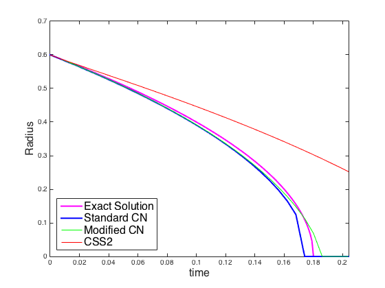
We know that BDF2 is a linear scheme so that satisfies the convexity property. Similar to the argument for the CSS version of modified Crank-Nicolson scheme (4.7), we know that (4.14) also satisfies the convexity property. When $k_{n}\leq\epsilon^{2}$ , these second-order splitting schemes perform well (see Test 11 below). However, we observe the following phenomenon for these second-order splitting schemes:

1.

They do not satisfy the discrete maximum principle, and it is frequently worse than the first-order scheme;
2.

They still suffer the lagging phenomenon or delayed convergence for large time step size (see Test 11 below);

Test 11

In this test, the same domain and initial conditions are chosen as in Test 1. Figure 4.5a shows the evolution of the radius with respect to time for different second-order schemes. We observe that all these second-order schemes perform well when $k_{n}=\epsilon^{2}$ . The performance of standard and modified Crank-Nicolson schemes are similar. When increasing the time step size, however, we observe that the lagging phenomenon exists for the CSS2 (see Figure 4.5b).

4.4 Artificial convexity

Following §2.4, the concept of artificial convexity scheme can also be applied to the wildly used CSS2 (4.14) by considering the following modified model:

u_{t}+\frac{\delta_{n}}{\epsilon^{2}}u_{tt}-\Delta u+\frac{1}{\epsilon^{2}}f(u)=0.

(4.15)

The modified Crank-Nicolson of (4.15) can be written as

	$\displaystyle(\frac{u_{h}^{n}-u_{h}^{n-1}}{k_{n}},v_{h})$	$\displaystyle+(\frac{\delta_{n}}{\epsilon^{2}}\cdot\frac{u_{h}^{n}-2u_{h}^{n-1}+u_{h}^{n-2}}{k_{n}^{2}},v_{h})$
		$\displaystyle+(\frac{\nabla u_{h}^{n}+\nabla u_{h}^{n-1}}{2},\nabla v_{h})+\frac{1}{\epsilon^{2}}(\tilde{F}[u_{h}^{n},u_{h}^{n-1}],v_{h})=0\qquad\forall v_{h}\in V_{h},$

which is exactly the CSS2 scheme (4.14) when $\delta_{n}=\frac{k_{n}^{2}}{2}$ .

5 Concluding remarks

In this paper, we mainly focus on how the behavior of numerical schemes depend on the time-step size. For a given finite element mesh, we compare solutions of fully discrete schemes with moderately small time step size with those of fully implicit schemes with extremely small time step size (which can be practically regarded as a reliable approximation of a semi-discretization scheme). We reach the following conclusions:

1.

A first-order CSS can be mathematically interpreted as a standard FIS with a (much) smaller time-step size. As a result, a CSS would usually lead to approximation of the solution of the original model at a delayed time. For the Allen-Cahn model, we have easily proved this time-delay effect rigorously. For the Cahn-Hilliard model, we observe that, from the numerical experiments, CSS also has a similar time-delay effect. This seems to indicate that the solution of the regularized model (2.28) will probably have a time-delay effect in comparison to the solution of the original Cahn-Hilliard model (1.2).
2.

Since CSS is really an FIS scheme in disguise (at least for the cases we have studied in this paper), the value of other FIS should not be under-estimated. Thus a modified FIS is proposed so that the maximum principle holds on the discrete level and, as a result, a Poisson-like preconditioner can be devised and rigorously analyzed.
3.

A major advantage of any partially implicit scheme is that a relatively large time-step size can be used; but such schemes with a large time-step size may have time delay (see Figure 4.5b) and hence may be inaccurate.
4.

By using energy minimization we can remove the constraint on the time step for fully implicit schemes without creating any delayed in the solutions.
5.

Through numerical experiments with modified Crank-Nicolson scheme, we showed that energy stable is not a sufficient condition (see Figure 4.2). That is, an unconditionally stable scheme is not necessarily better than a conditionally stable scheme.
6.

In summary, we recommend to use FIS with energy minimization.

While most partially implicit schemes have been developed as a numerical technique for solving a given phase-field model, given the insight obtained in this paper, we would like to argue that it may be helpful to view the convex splitting technique as a discrete modeling technique, namely a procedure to convexify the original model. The convexified models are (2.33) and (2.34) for the Allen-Cahn Model and the Cahn-Hilliard equation, respectively. While neither (2.33) nor (2.34) has a corresponding convexity property on the continuous level, their appropriately discretized model would have the desired “uniform convexity” properties as stated in Theorem 2.7.

Partially implicit schemes (especially CSS) have been used for many different models that are different from or more complicated than both the Allen-Cahn and Cahn-Hilliard equations. We have not studied carefully how these schemes behave in those models, but hopefully our findings in this paper on partially implicit schemes for both the Allen-Cahn and Cahn-Hilliard models will give some new insight into the nature of convex splitting technique.

In terms of the unconditional energy-stability, we presented an energy minimization version of the fully implicit schemes for phase field modeling. Although it is challenging to find the global minimizer, hopefully our findings in this paper on fully implicit schemes for both the Allen-Cahn and Cahn-Hilliard equations will give some new insight on the phase field modeling. Accordingly, the design of a fast solver for the energy minimization problem arising from the phase field modeling is a research topic of great theoretical and practical importance.

References

[1] A. Aristotelous, O. Karakashian and S. Wise, A mixed discontinuous Galerkin, convex splitting scheme for a modified Cahn-Hilliard equation and an efficient nonlinear multigrid solver, DCDS-B, 18, 2211–2238, 2013.
[2] N. D. Alikakos, P. W. Bates, and X. Chen, Convergence of the Cahn-Hilliard equation to the Hele-Shaw model, Arch. Rational Mech. Anal., 128(2):165–205, 1994.
[3] S. Allen and J. W. Cahn, A microscopic theory for antiphase boundary motion and its application to antiphase domain coarsening, Acta Metall., 27, 1084–1095, 1979.
[4] F. Boyer and S. Minjeaud, Hierarchy of consistent n-component Cahn–Hilliard systems, Math. Models Methods Appl. Sci., 24(14), 2885–2928, 2014.
[5] R. H. Byrd, P. Lu, J. Nocedal and C. Zhu, A limited memory algorithm for bound constrained optimization, SIAM J. Sci. Comput., 16(5), 1190–1208, 1995.
[6] J. W. Cahn and A. Novick-Cohen, Limiting motion for an Allen-Cahn/Cahn-Hilliard system, Free Boundary Prob., Theory Appl., 363, 89–97, 1996.
[7] J. W. Cahn and J. E. Hilliard, Free energy of a nonuniform system I. Interfacial free energy, J. Chem. Phys., 28, 258–267, 1958.
[8] L. Chen, iFEM: An integrated finite element methods package in MATLAB, technical report, University of California Irvine, 2008.
[9] X. Chen, Spectrums for the Allen-Cahn, Cahn-Hilliard, and phase-field equations for generic interface, Comm. Partial Diff Eqns, 19:1371–1395, 1994.
[10] X. Chen, Global asymptotic limit of solutions of the Cahn-Hilliard equation, J. Diff. Geom., 44(2):262–311, 1996.
[11] X. Chen and G. Caginalp, Convergence of the phase field model to its sharp interface limits, Eur. J. Appl. Math., 9(04):417–445, 1998.
[12] P. Ciarlet, B. Miara and T. Jean-Marie, Introduction to numerical linear algebra and optimisation, Cambridge University Press, 1989.
[13] N. Condette, C. Melcher and E. Süli, Spectral approximation of pattern-forming nonlinear evolution equations with double-well potentials of quadratic growth, Math. Comp., 80(273), 205–223, 2011.
[14] D. Gilbarg and N. Trudinger, Elliptic partial differential equations of second order, Springer, 2015.
[15] Q. Du and R. Nicolaides, Numerical analysis of a continuum model of phase transition, SIAM J. Numer. Anal., 28(5): 1310–1322, 1991.
[16] L. C. Evans, H. n. Soner, and P. E. Souganidis, Phase transitions and generalized motion by mean curvature, Comm. Pure Appl. Math., 45(9), 1097–1123, 1992.
[17] D. Eyre, Unconditionally gradient stable time marching the Cahn-Hilliard equation, in Computational and Mathematical Models of Microstructural Evolution, J. W. Bullard, R. Kalia, M. Stoneham, and L. Q. Chen, eds., Mater. Res. Soc. Symp. Proc. 529, Materials Research Society, Warrendale, PA, 39–46, 1998.
[18] X. Feng, Y. He and C. Liu, Analysis of finite element approximations of a phase field model for two-phase fluids, Math. Comp., 76(258), 539–571, 2007.
[19] X. Feng and Y. Li, Analysis of interior penalty discontinuous Galerkin methods for the Allen-Cahn equation and the mean curvature flow, IMA J. Numer. Anal., 35(4), 1622-1651, 2015.
[20] X. Feng, Y. Li, and Y. Xing, Analysis of mixed interior penalty discontinuous Galerkin methods for the Cahn-Hilliard equation and the Hele-Shaw flow, SIAM J. Numer. Anal., 54(2), 825–847, 2016.
[21] X. Feng and A. Prohl, Numerical analysis of the Allen-Cahn equation and approximation for mean curvature flows, Numer. Math., 94, 33–65, 2003.
[22] X. Feng and T. Tang, and J. Yang, Long time numerical simulations for phase-field problems using p-adaptive spectral deferred correction methods, Numer. Math., 94, 33–65, 2003.
[23] X. Feng and H. Wu, A posteriori error estimates and an adaptive finite element method for the Allen–Cahn equation and the mean curvature flow, J. Sci. Comput., 24(2), 121–146, 2005.
[24] H. Gòmez, V. M. Calo, Y. Bazilevs, and T. J.R. Hughes, Isogeometric analysis of the Cahn–Hilliard phase-field model, Computer Methods in Applied Mechanics and Engineering, 197 (49), 4333-4352, 2008.
[25] C. Gräser, R. Kornhuber and U. Sack, Time discretization of anisotropic Allen–Cahn equations, IMA J. Numer. Anal., 33(4), 1226–1244, 2013.
[26] Z. Guan, J. S. Lowengrub, C. Wang and S. N. Wise, Second order convex splitting schemes for periodic nonlocal Cahn–Hilliard and Allen–Cahn equations, J. Comput. Phys., 277, 2014.
[27] F. Guillén-González and G. Tierra, Second order schemes and time-step adaptivity for Allen–Cahn and Cahn–Hilliard models, Comput. Math. Appl., 68(8), 821–846, 2014.
[28] P. Hartman, On functions representable as a difference of convex functions, Pacific J. Math, 9(3), 707-713, 1959.
[29] T. Ilmanen, Convergence of the Allen-Cahn equation to Brakke’s motion by mean curvature, J. Diff. Geom., 38(2), 417–461, 1993.
[30] J. Kim, K. Kang and J. Lowengrub, Conservative multigrid methods for Cahn–Hilliard fluids, J. Comput. Phys., 193, 2004.
[31] Y. Li, Numerical methods for deterministic and stochastic phase field models of phase transition and related geometric flows, Ph.D. thesis, University of Tennessee, 2015.
[32] J. Nocedal, Updating quasi-Newton matrices with limited storage, Math. Comp., 35(151), 773–782, 1980.
[33] R. H. Nochetto and C. Verdi, Combined effect of explicit time-stepping and quadrature for curvature driven flows, Numer. Math., 74(1), 1996.
[34] R. H. Nochetto and C. Verdi, Convergence past singularities for a fully discrete approximation of curvature-driven interfaces, SIAM J. Numer. Anal., 34(2), 490–512, 1997.
[35] A. Novick-Cohen, The Cahn-Hilliard equation: Mathematical and modeling perspectives, Adv. Math. Sci. Appl., 8:965–985, 1998.
[36] R. L. Pego, Front migration in the nonlinear Cahn-Hilliard equation, Proc. Roy. Soc. London Ser. A, 422(1863), 107–145, 1989.
[37] J. Rosam, P. K. Jimack and A. Mullis, A fully implicit, fully adaptive time and space discretisation method for phase-field simulation of binary alloy solidification, J. Comput. Phys., 255(2), 1271–1287, 2007.
[38] J. Shen, T. Tang and L. Wang, Spectral methods: algorithms, analysis and applications, Springer Science & Business Media, 41, 2011.
[39] J. Shen, T. Tang and J. Yang, On the maximum principle preserving schemes for the generalized Allen-Cahn Equation, preprint, 2014.
[40] J. Shen and X. Yang, Numerical approximations of Allen-Cahn and Cahn-Hilliard equations, Discrete Contin. Dyn. Syst., 28(4), 2010.
[41] J. Shen and X. Yang, Energy stable schemes for Cahn-Hilliard phase-field model of two-phase incompressible flows, Chin. Ann. Math., Series B, 31(5), 743–758, 2010.
[42] G. Strang and G. J. Fix, An analysis of the finite element method, Prentice-Hall Englewood Cliffs, N. J., 1973.
[43] X. Tai and J. Xu, Global and uniform convergence of subspace correction methods for some convex optimization problems, Math. Comp., 71(237), 105–124, 2002.
[44] S. Wise, J. Kim and J. Lowengrub, Solving the regularized, strongly anisotropic Cahn–Hilliard equation by an adaptive nonlinear multigrid method, J. Comput. Phys., 226, 414–446, 2007.
[45] S. Wu and J. Xu, Multiphase Allen–Cahn and Cahn–Hilliard models and their discretizations with the effect of pairwise surface tensions, J. Comput. Phys., 343, 10–32, 2017.
[46] J. Xu and L. Zikatanov, A monotone finite element scheme for convection-diffusion equations, Math. Comp., 68(228), 1429–1446, 1999.
[47] X. Yang, Error analysis of stabilized semi-implicit method of Allen-Cahn equation, Discrete Contin. Dyn. Syst. Ser. B, 11(4), 2009.

On the Stability and Accuracy of Partially and Fully Implicit Schemes for Phase Field Modeling

Abstract

Keywords:

1 Introduction

2 First-order schemes

2.1 Fully implicit schemes and their convexity and energy stability properties

2.1.1 Convexity of fully implicit schemes for the Allen-Cahn equation

Theorem 2.1.

Proof.

2.1.2 Convexity of fully implicit scheme for the Cahn-Hilliard equation

Theorem 2.2.

Proof.

2.2 Convex splitting schemes and their equivalence to fully implicit schemes

2.2.1 A convex splitting scheme for the Allen-Cahn model

Theorem 2.3.

Theorem 2.4.

Proof.

Remark 2.1.

Test 1

Test 2

Test 3

2.2.2 A convex splitting scheme for the Cahn-Hilliard model

Theorem 2.5.

Test 4

2.3 Some other first-order partially implicit schemes

Theorem 2.6.

Proof.

Test 5

2.4 Convex splitting schemes interpreted as artificial convexity schemes

Theorem 2.7.

Proof.

3 A modified FIS satisfying a discrete maximum principle

3.1 A modified scheme

Theorem 3.1.

Theorem 3.2.

Proof.

Test 6

Remark 3.1.

Remark 3.2.

3.2 A robust preconditioner for the Allen-Cahn equation

Theorem 3.3.

Proof.

Theorem 3.4.

Remark 3.3.

Test 7

4 Second-order schemes

4.1 (Modified) Crank-Nicolson scheme for the Allen-Cahn equation

Theorem 4.1.

Proof.

Lemma 4.2 ([40, 13]).

Proof.

Theorem 4.3.

Proof.

Remark 4.1.

Test 8

Test 9

Test 10

4.2 Modified Crank-Nicolson scheme for the Cahn-Hilliard equation

Lemma 4.4 ([13, 40]).

Proof.

Theorem 4.5.

Proof.

Remark 4.2.

4.3 Some other second-order partially implicit schemes

Test 11

4.4 Artificial convexity

5 Concluding remarks

References

References

On the Stability and Accuracy of Partially and Fully
Implicit Schemes for Phase Field Modeling