跳到论文正文
W Papers独立论文阅读器 arXiv:1604.05268 论文正文 计算阅读时间 · 0%
引用这篇论文根据当前论文元数据生成,正式投稿前建议核对。


License: arXiv.org perpetual non-exclusive license
arXiv:1604.05268v2 [math.NA] 24 May 2016

A partial Fourier transform method for a class of
hypoelliptic Kolmogorov equations

C. Reisinger Note: Mathematical Institute, University of Oxford, Andrew Wiles Building, Woodstock Rd., Oxford OX2 6GG, {reisinge, suli, whitley}@maths.ox.ac.uk    E. Süli††footnotemark:    A. Whitley††footnotemark:
Abstract

We consider hypoelliptic Kolmogorov equations in n+1n+1 spatial dimensions, with n≥1n\geq 1, where the differential operator in the first nn spatial variables featuring in the equation is second-order elliptic, and with respect to the (n+1)(n+1)st spatial variable the equation contains a pure transport term only and is therefore first-order hyperbolic. If the two differential operators, in the first nn and in the (n+1)(n+1)st co-ordinate directions, do not commute, we benefit from hypoelliptic regularization in time, and the solution for t>0t>0 is smooth even for a Dirac initial datum prescribed at t=0t=0. We study specifically the case where the coefficients depend only on the first nn variables. In that case, a Fourier transform in the last variable and standard central finite difference approximation in the other variables can be applied for the numerical solution. We prove second-order convergence in the spatial mesh size for the model hypoelliptic equation ∂u∂t+x​∂u∂y=∂2u∂x2\frac{\partial u}{\partial t}+x\frac{\partial u}{\partial y}=\frac{\partial^{2}u}{\partial x^{2}} subject to the initial condition u⁡(x,y,0)=δ⁡(x)⊗δ⁡(y)u(x,y,0)=\delta(x)\otimes\delta(y), with (x,y)∈ℝ×ℝ(x,y)\in\mathbb{R}\times\mathbb{R} and t>0t>0, proposed by Kolmogorov, and for an extension with n=2n=2. We also demonstrate exponential convergence of an approximation of the inverse Fourier transform based on the trapezium rule. Lastly, we apply the method to a PDE arising in mathematical finance, which models the distribution of the hedging error under a mis-specified derivative pricing model.

AMS Subject Classification: 65N06, 35H10, 35Q84, 65T50

Keywords: Hypoelliptic equations, Kolmogorov equation, Dirac initial datum, Fourier methods, finite difference methods

1 Introduction

This paper is concerned with the numerical solution of initial-value problems for a class of partial differential equations, subject to Dirac initial datum, which have the form

∂u∂t+c⁡(x,t)​∂u∂y\displaystyle\frac{\partial u}{\partial t}+c(x,t)\frac{\partial u}{\partial y} =ℒ​u,\displaystyle=\mathcal{L}u, (x,y,t)∈ℝn×ℝ×(0,T],\displaystyle\qquad(x,y,t)\in\mathbb{R}^{n}\times\mathbb{R}\times(0,T], (1.1)
u⁡(x,y,0)\displaystyle u(x,y,0) =δ⁡(x−x0)⊗δ⁡(y−y0),\displaystyle=\delta(x-x_{0})\otimes\delta(y-y_{0}), (x,y)∈ℝn×ℝ,\displaystyle\qquad(x,y)\in\mathbb{R}^{n}\times\mathbb{R}, (1.2)

where n≥1n\geq 1, T>0T>0, x0∈ℝnx_{0}\in\mathbb{R}^{n}, y0∈ℝy_{0}\in\mathbb{R}, the symbol ⊗\otimes signifies the (associative) binary operation of tensor product of distributions, the drift coefficient c=c⁡(x,t)c=c(x,t) is independent of the variable y∈ℝy\in\mathbb{R}, ∇xc​(x,t)≠0\nabla_{x}c(x,t)\neq 0 for all (x,t)∈ℝn×(0,T](x,t)\in\mathbb{R}^{n}\times(0,T], the elliptic differential operator ℒ\mathcal{L} does not include any yy-derivatives and its coefficients only depend on x=(x1,…,xn)∈ℝnx=(x_{1},\dots,x_{n})\in\mathbb{R}^{n} and t∈[0,T]t\in[0,T]; in other words, ℒ\mathcal{L} is assumed to be of the form

ℒ=∑i,j=1nai​j​(x,t)​∂2∂xi​∂xj+∑i=1nbi​(x,t)​∂∂xi+d⁡(x,t),\displaystyle\mathcal{L}=\sum_{i,j=1}^{n}a_{ij}(x,t)\frac{\partial^{2}}{\partial x_{i}\partial x_{j}}+\sum_{i=1}^{n}b_{i}(x,t)\frac{\partial}{\partial x_{i}}+d(x,t), (1.3)

where ai​ja_{ij}, i,j=1,…,ni,j=1,\dots,n, bib_{i}, i=1,…​ni=1,\dots n, and dd are continuous functions of (x,t)∈ℝn×[0,T](x,t)\in\mathbb{R}^{n}\times[0,T], and there exists a constant c0>0c_{0}>0 such that

∑i,j=1nai​j​(x,t)​ξi​ξj≥c0​|ξ|2∀ξ=(ξ1,…,ξn)∈ℝn∀(x,t)∈ℝn×[0,T].\sum_{i,j=1}^{n}a_{ij}(x,t)\xi_{i}\xi_{j}\geq c_{0}|\xi|^{2}\qquad\forall\,\xi=(\xi_{1},\dots,\xi_{n})\in\mathbb{R}^{n}\quad\forall\,(x,t)\in\mathbb{R}^{n}\times[0,T].

Hypoelliptic problems of this kind arise naturally from statistical physics, stochastic analysis, and from mathematical finance in particular, as Kolmogorov equations that describe the evolution of the probability density function of stochastic processes, and the initial datum in such problems is frequently a point source, which is modelled by a Dirac measure concentrated at a point. Such initial conditions are clearly also relevant in the construction of Green’s functions.

For the definition of hypoellipticity and sufficient and necessary conditions for C∞C^{\infty} regularity see [5]. Contemporary applications and extensions to nonlinear problems are found in [16, 17].

Given the interest in this class of equations, methods have recently been put forward for their numerical approximation, with a focus on preserving the long-time behaviour of solutions to the original equation. In [2], a self-similar change of variables was performed and convergence of the numerical solution to the steady state under these new variables was established; furthermore, an operator splitting scheme based on decomposing the hypoelliptic operator into coercive and convective terms was proposed. In contrast, in [12] asymptotic properties of standard central finite difference schemes are analyzed and decay rates of difference quotients were proved in the case of L2L^{2} initial data. The analysis in those papers does not cover the case of Dirac initial data, which are important in a number of applications, and indeed the numerical experiments at the end of this section show that in the case of Dirac initial datum convergence of a finite difference approximation to the problem based on central differences is not guaranteed in the discrete maximum norm.

The semidiscrete Fourier scheme that we propose here for the numerical approximation of problem (1.1) involves the application of a Fourier transform to (1.1) in the yy-direction (yy-FT) to reduce the dimension of the problem by transforming it into a one-parameter family of parabolic problems, and it then applies finite difference discretization in the xx-direction to this parametrized family of parabolic problems, followed by the application of an inverse Fourier transform. The observed exponential convergence of the numerical approximation to the inverse Fourier transform reduces the computational complexity of the proposed scheme to that of a finite difference approximation of a problem that has no dependence on yy, as long as the solution is required for a single value of yy only. The application of the yy-FT avoids the use of lower-order stable upwind or semi-Lagrangian discretizations of the yy-derivative. Moreover, it transforms the Dirac initial datum into a constant function in the yy-direction, which is easier to handle numerically. To the best of our knowledge, the numerical scheme proposed in this paper is the first provably convergent numerical method for hypoelliptic problems of this type, with Dirac initial datum.

We shall study in-depth the stylized problem

∂u∂t+x​∂u∂y\displaystyle\frac{\partial u}{\partial t}+x\frac{\partial u}{\partial y} =∂2u∂x2,\displaystyle=\frac{\partial^{2}u}{\partial x^{2}}, (x,y,t)∈ℝ×ℝ×(0,T],\displaystyle\qquad(x,y,t)\in\mathbb{R}\times\mathbb{R}\times(0,T], (1.4)
u⁡(x,y,0)\displaystyle u(x,y,0) =δ⁡(x)⊗δ⁡(y),\displaystyle=\delta(x)\otimes\delta(y), (x,y)∈ℝ×ℝ.\displaystyle\qquad(x,y)\in\mathbb{R}\times\mathbb{R}. (1.5)

This is the partial differential equation originally considered by Kolmogorov in his 1934 paper [8]. The significance of this simple model problem stems from the fact that it incorporates two important features: hypoellipticity and Dirac initial datum. The equation (1.4) results from (1.3) for d≡0d\equiv 0 by shifting the point (x0,y0)(x_{0},y_{0}) at which the initial Dirac datum is concentrated to the origin, linearization of the coefficient cc with respect to the yy variable around y=0y=0, translation in the yy-direction with c⁡(0,0)​tc(0,0)t, and finally freezing the coefficients cc, bb and aa with respect to tt. Since the final term in (1.3) does not affect the ideas presented herein, for the sake of simplicity of the exposition we shall confine ourselves to the case of d≡0d\equiv 0. Subject to sign change, our model equation (1.4) coincides with the one studied in [12].

Because of the special structure of the equation (1.4), we shall apply Fourier methods in the construction of its numerical approximation and also in the convergence analysis of the proposed numerical algorithms. We shall explore the behaviour of two numerical schemes for the solution of our model problem: a semidiscrete Fourier method and a fully-discrete Fourier method, which will be described below.

Whereas the proposed numerical techniques apply to the more general model problem (1.1), (1.2), and, in fact, with more general probability measures as initial data than the Dirac measure considered herein, for the sake of simplicity and clarity of the exposition the mathematical analysis of the proposed numerical methods is restricted to the simplified model (1.4), (1.5), which is a special case of the Cauchy problem (1.1), (1.2) above. For this toy model, we shall prove the convergence of the semidiscrete Fourier method and derive expressions for the leading order terms for the global discretization error. In particular, we shall analyze the behaviour of the error between the analytical solution and its numerical approximation and will establish the rate of convergence of the scheme as the spatial discretization parameter Δ​x→0\Delta x\rightarrow 0. It should be noted that this analysis only relates to the analytical solution of the semidiscrete scheme (2.7) and its subsequent exact yy-FT inversion. We shall discuss these additional approximations in Section 4.

We approach the task of error analysis by applying the inverse Fourier transform to the error between WW and ww, where WW is the solution of the equation resulting from Fourier transforming (1.4) with respect to yy, discretizing with respect to xx, and applying a discrete Fourier transform with respect to xx, whereas ww is the solution of the equation resulting from Fourier transforming (1.4) with respect to both xx and yy. We then perform a wavenumber analysis of the resulting expressions to establish convergence. This method is based on similar ideas to those in [1] and [13], where time-stepping schemes for the one-dimensional heat equation with Dirac initial datum were analyzed. While in the cited papers the Fourier transform was used purely as a mathematical tool in the analysis of the discretization error in the original space-time co-ordinates, here we use a partial Fourier transform (i.e., we transform in the yy-variable only) in the construction of the actual numerical method and use a double-Fourier transform (i.e., the Fourier transform in both the xx and the yy variable) to quantify the error of this approximation. An interesting feature of the present analysis is the intricate interplay between the xx- and yy-Fourier modes, due to the hypoellipticity of the equation.

In order to motivate the numerical method proposed in the next section, we illustrate the smoothing and convergence properties of the central difference scheme with implicit Euler time stepping,

Uj,kn+1−Uj,knΔ​t+xj​Uj,k+1n+1−Uj,k−1n+12​Δ​y=Uj+1,kn+1−2​Uj,kn+1+Uj−1,kn+1Δ​x2,with (j,k)∈ℤ2 and n≥0.\displaystyle\frac{U_{j,k}^{n+1}-U_{j,k}^{n}}{\Delta t}+x_{j}\frac{U_{j,k+1}^{n+1}-U_{j,k-1}^{n+1}}{2\Delta y}=\frac{U_{j+1,k}^{n+1}-2U_{j,k}^{n+1}+U_{j-1,k}^{n+1}}{\Delta x^{2}},\qquad\mbox{with $(j,k)\in\mathbb{Z}^{2}$ and $n\geq 0$.}

This is the scheme studied in [12]; it is shown there in particular that, for ℓ2\ell^{2} initial data, the ℓ2\ell^{2} norms of the first-order difference quotients in the xx- and yy-directions decay as t−1t^{-1} and t−3t^{-3}, respectively, as t→∞t\rightarrow\infty. Closer to the situation in the present paper, let us consider, instead, a Dirac delta concentrated at the origin in the (x,y)(x,y)-plane. We approximate the Dirac initial datum by

Uj,k0={1Δ​x​Δ​yfor (j,k)=(0,0),0for (j,k)≠(0,0),(j,k)∈ℤ2,\displaystyle U_{j,k}^{0}=\left\{\begin{array}[]{cl}\frac{1}{\Delta x\,\Delta y}&\mbox{for $(j,k)=(0,0)$,}\\ 0&\mbox{for $(j,k)\neq(0,0)$},\end{array}\right.\qquad(j,k)\in\mathbb{Z}^{2},

which can be viewed as the mollification of the Dirac measure concentrated at the origin through convolution, in the sense of distributions, with the scaled characteristic function 1Δ​x​Δ​yχ[−Δx/2,Δx/2]×[−Δy/2,Δy/2]\frac{1}{\Delta x\,\Delta y}\chi_{[-\Delta x/2,\Delta x/2]\times[-\Delta y/2,\Delta y/2]} with unit L1L^{1} norm (cf. [6]). We shall consider the problem on a sufficiently large square domain (−L,L)×(−L,L)(-L,L)\times(-L,L) in the (x,y)(x,y)-plane, with zero Dirichlet boundary condition along (±L,y)(\pm L,y) for all y∈[−L,L]y\in[-L,L] and along (x,−L)(x,-L) for all x∈[−L,L]x\in[-L,L]; in our numerical experiment below we took L=10L=10, which ensures that the Dirichlet boundary condition has negligible influence on the values of the numerical solution at the final time of interest, T=1T=1 in our case, close to the centre of the square where the initial Dirac delta is concentrated.

Fig. 1, left, shows the numerical solution at T=1T=1, which exhibits large oscillations in the xx-direction, but is smooth in the yy-direction. Indeed, good approximation to the analytical solution is visible between the oscillations. The discrete Fourier transform of the numerical solution, with wavenumbers ss and pp (described in more detail later), is depicted in the right panel in Fig. 1. It shows low wavenumber components in both ss and pp near the origin in Fourier space, which approximate well the Fourier transform of the analytical solution, and low ss-/high pp-wavenumber components concentrated at (s,p)=(0,±π/Δy)=(0,±20π)≈(0,±63)(s,p)=(0,\pm\pi/\Delta y)=(0,\pm 20\pi)\approx(0,\pm 63), which trigger the spurious oscillations in the numerical approximation of the analytical solution.

Figure 1: Central difference scheme with Dirac initial datum; the computational domain is x∈[−10,10]x\in[-10,10], y∈[−10,10]y\in[-10,10] (smaller plot range); the numerical solution at T=1T=1 with nx=ny=nt=400n_{x}=n_{y}=n_{t}=400 grid spacings in the xx-, yy-, and tt-directions, respectively; left the numerical solution, right its discrete Fourier transform, with ss and pp signifying wavenumbers corresponding to the xx and yy co-ordinate directions, respectively.
Refer to caption
Refer to caption

Extending the techniques from [1], the time-discrete evolution of the discrete Fourier transform WW of the numerical solution UU is found to be governed by the recursion (see also Sections 3.1 and especially 4.5)

(1+4​Δ​tΔ​x2​sin2⁡(s​Δ​x2))​Wn+1​(s,p)\displaystyle\left(1+4\frac{\Delta t}{\Delta x^{2}}\sin^{2}\left(\frac{s\Delta x}{2}\right)\right)W^{n+1}(s,p) =Wn​(s,p)+Δ​tΔ​y​sin⁡(p​Δ​y)​∂Wn+1∂s​(s,p),n≥0,\displaystyle=W^{n}(s,p)+\frac{\Delta t}{\Delta y}\sin(p\Delta y)\frac{\partial W^{n+1}}{\partial s}(s,p),\qquad n\geq 0,
W0​(s,p)\displaystyle W^{0}(s,p) =1,\displaystyle=1,

for all (s,p)∈[−πΔ​x,πΔ​x]×[−πΔ​y,πΔ​y](s,p)\in[-\frac{\pi}{\Delta x},\frac{\pi}{\Delta x}]\times[-\frac{\pi}{\Delta y},\frac{\pi}{\Delta y}]. Setting s=0s=0 and p=±π/Δyp=\pm\pi/\Delta y we deduce that

Wn(0,±π/Δy)=1∀n≥1.\displaystyle W^{n}(0,\pm\pi/\Delta y)=1\qquad\forall\,n\geq 1.

This finding is in line with our numerical simulations, and suggests that the numerical solution will not converge to the analytical solution as Δ​x,Δ​y→0\Delta x,\Delta y\rightarrow 0. To reconcile this evidence with the results in [12], we compute a numerical approximation to the solution at T=2T=2, starting with the exact (smooth) solution (see (4.5)) as initial datum at t=1t=1. The numerical solution and its discrete Fourier transform are shown in Fig. 2.

As the initial datum in this case does not have high wavenumber components, the numerical solution approximates the analytical solution well. Indeed, the maximum error is around 1.8×10−41.8\times 10^{-4} (solution ≈0.07\approx 0.07), compared to 0.280.28 (solution ≈0.3\approx 0.3) for the Dirac case.

Replacing the central yy-difference with an upwind yy-difference is observed to produce a convergent sequence of numerical approximations to the analytical solution in the case of a Dirac initial datum, just as for smooth initial data, but such a finite difference scheme is only of first-order accuracy with respect to Δ​y\Delta y. We shall therefore propose in the next section a numerical scheme applied to the analytical yy-Fourier transform, which does not suffer from this shortcoming.

Figure 2: Central difference scheme with smooth initial datum: x∈[−10,10]x\in[-10,10], y∈[−10,10]y\in[-10,10], t∈[1,2]t\in[1,2], nx=ny=nt=400n_{x}=n_{y}=n_{t}=400; the numerical solution at T=2T=2 (left) and its discrete Fourier transform (right).
Refer to caption
Refer to caption

The remainder of the article is structured as follows. In Section 2 we introduce the semidiscrete Fourier scheme and formulate the discretization of the model problem (1.4), (1.5); in Section 3 we prove that the scheme is second-order convergent in Δ​x\Delta x in the space-time ℓ∞\ell^{\infty} norm. Next, in Section 4, we describe aspects of the numerical implementation including the exponential convergence in Δ​p\Delta p, the mesh size of the Fourier variable in the yy-direction, and present numerical results for the model problem (1.4), (1.5). In Section 5, we discuss the application of the method to a financial hedging problem, while Section 6 is concerned with the convergence analysis of the extension of the scheme to the case of n=2n=2, i.e. the diffusion operator acts in two spatial directions, x=(x1,x2)x=(x_{1},x_{2}), while in the third spatial direction, yy, there is only a transport term present in the equation; in other words, there is no diffusion in the yy-direction. Our findings are summarized in the concluding section.

2 The semidiscrete Fourier scheme

The Fourier transform in the yy-direction (briefly, yy-FT) is defined by

v⁡(x,p,t):=∫−∞∞u⁡(x,y,t)​ei​p​y​𝑑y,x∈ℝ,p∈ℝ,t>0.v(x,p,t):=\int^{\infty}_{-\infty}u(x,y,t)\,{\rm e}^{ipy}\,{\rm d}y,\qquad x\in\mathbb{R},\;p\in\mathbb{R},\;t>0.

where it is tacitly understood that the function y∈ℝ↦u⁡(x,y,t)∈ℝy\in\mathbb{R}\mapsto u(x,y,t)\in\mathbb{R} is an element of L1​(ℝ)L^{1}(\mathbb{R}) for all (x,t)∈ℝn×(0,∞)(x,t)\in\mathbb{R}^{n}\times(0,\infty). The Fourier transform in the yy-direction of the initial Dirac measure δ⁡(x−x0)⊗δ⁡(y−y0)\delta(x-x_{0})\otimes\delta(y-y_{0}) at t=0t=0 is to be understood in the sense of distributions, and is equal to δ⁡(x−x0)⊗ei​p​y0\delta(x-x_{0})\otimes{\rm e}^{ipy_{0}}.

Application of the Fourier transform to (1.1) yields

∂v∂t−i​p​c​(x,t)​v=ℒ​vx∈ℝ,p∈ℝ,t>0,\frac{\partial v}{\partial t}-ipc(x,t)v=\mathcal{L}v\qquad x\in\mathbb{R},\;p\in\mathbb{R},\;t>0,

which is a family of PDEs in xx and tt, parametrized by pp, for the yy-FT: v⁡(x,p,t)v(x,p,t). We then discretize the operator ℒ\mathcal{L} from (1.3) in the xx-direction(s) by means of a standard finite difference scheme, using equally spaced grid points, with spacing Δ​x\Delta x, but we keep the time variable continuous for the moment at least. This leads to a system of ordinary differential equations (ODEs) indexed by the xx-grid points, xjx_{j}, and also by the Fourier wavenumber in the yy-direction, which we are denoting by pp, for the function Vj​(p,t)V_{j}(p,t). After solving this system of ODEs (in practice numerically, for a finite set of grid points xjx_{j} subject to an artificial/numerical Dirichlet boundary condition at the ‘far-field’, and a finite set of yy-wave numbers, OPEN{pl}l=lm​i​nlm​a​x)\{p_{l}\}_{l=l_{min}}^{l_{max}}), we use the inverse yy-FT to obtain an approximate solution, U⁡(xj,y,t)U(x_{j},y,t), in the original co-ordinates as

U(xj,y,t)=12​π∫−2t/(Δx)r2​t/(Δ​x)rVj(p,t)e−i​y​pdp.\displaystyle U(x_{j},y,t)=\frac{1}{2\pi}\int^{2t/(\Delta x)^{r}}_{-2t/(\Delta x)^{r}}V_{j}(p,t)\,{\rm e}^{-iyp}\,{\rm d}p. (2.1)

The truncation of the pp-integration range in the inversion (2.1) from p∈(−∞,∞)p\in(-\infty,\infty) to the truncated range p∈(−2t/(Δx)r,2t/(Δx)r)p\in(-2t/(\Delta x)^{r},2t/(\Delta x)^{r}), for a suitable r>0r>0, is dictated by the practical requirement to carry out numerical integration over a finite range. The scaling with 2​t2t simplifies the numerical analysis, but of course in practice any suitable scaling would be chosen empirically.

To find the approximation Uj,k​(t)U_{j,k}(t) to u⁡(xj,yk,t)u(x_{j},y_{k},t) numerically, we apply a uniformly spaced and equally weighted quadrature rule to (2.1) and obtain

Uj,k​(t):=Δ​p2​π​∑l=lm​i​nlm​a​xVj​(pl,t)​e−i​yk​pl\displaystyle U_{j,k}(t):=\frac{\Delta p}{2\pi}\sum^{l_{max}}_{l=l_{min}}V_{j}(p_{l},t)\,{\rm e}^{-iy_{k}p_{l}} (2.2)

for a given kk, lm​a​x>0l_{max}>0, lm​i​n<0l_{min}<0, lm​a​x​Δ​p=−lm​i​n​Δ​p=2​t​Δ​x−rl_{max}\Delta p=-l_{min}\Delta p=2t\Delta x^{-r}. We will also denote np:=lm​a​x−lm​i​n+1n_{p}:=l_{max}-l_{min}+1. The numerical results will be seen to exhibit exponential convergence of the pp-quadrature (see below and [15]). For an efficient implementation of (2.2), if the solution is needed for several values of kk, the Fast Fourier Transform (FFT) can be used.

We illustrate the method by applying it to the Cauchy problem

∂u∂t+x​∂u∂y\displaystyle\frac{\partial u}{\partial t}+x\frac{\partial u}{\partial y} =∂2u∂x2,\displaystyle=\frac{\partial^{2}u}{\partial x^{2}}, (x,y,t)∈ℝ×ℝ×(0,T],\displaystyle\qquad(x,y,t)\in\mathbb{R}\times\mathbb{R}\times(0,T], (2.3)
u⁡(x,y,0)\displaystyle u(x,y,0) =δ⁡(x)⊗δ⁡(y),\displaystyle=\delta(x)\otimes\delta(y), (x,y)∈ℝ×ℝ,\displaystyle\qquad(x,y)\in\mathbb{R}\times\mathbb{R}, (2.4)

with the aim to analyze the stability and accuracy of the numerical scheme we develop below.

Applying the yy-FT to (2.3) we get

∂v∂t−i​p​x​v\displaystyle\frac{\partial v}{\partial t}-ipxv =∂2v∂x2,\displaystyle=\frac{\partial^{2}v}{\partial x^{2}}, (x,p,t)∈ℝ×ℝ×(0,T],\displaystyle\qquad(x,p,t)\in\mathbb{R}\times\mathbb{R}\times(0,T], (2.5)
u⁡(x,p,0)\displaystyle u(x,p,0) =δ⁡(x),\displaystyle=\delta(x), (x,p)∈ℝ×ℝ,\displaystyle\qquad(x,p)\in\mathbb{R}\times\mathbb{R}, (2.6)

and we then discretize this one-parameter family of Cauchy problems in the xx-direction only, using central differencing with spacing Δ​x>0\Delta x>0, to obtain, for xj=j​Δ​xx_{j}=j\Delta x, j∈ℤj\in\mathbb{Z},

∂Vj​(p,t)∂t−i​p​xj​Vj​(p,t)=Vj+1​(p,t)−2​Vj​(p,t)+Vj−1​(p,t)Δ​x2,p∈ℝ,t∈(0,T],\displaystyle\frac{\partial V_{j}(p,t)}{\partial t}-ipx_{j}V_{j}(p,t)=\frac{V_{j+1}(p,t)-2V_{j}(p,t)+V_{j-1}(p,t)}{\Delta x^{2}},\qquad p\in\mathbb{R},\;t\in(0,T], (2.7)

so that the function Vj​(p,t)V_{j}(p,t), which approximates v⁡(xj,p,t)v(x_{j},p,t), satisfies this equation for each j∈ℤj\in\mathbb{Z} and for all (p,t)∈ℝ×(0,T](p,t)\in\mathbb{R}\times(0,T]. The initial condition we use for this parametrized ODE system is

Vj​(p,0)={0 for ​j≠0,1Δ​x for ​j=0,\displaystyle V_{j}(p,0)=\left\{\begin{array}[]{cl}0&\text{ for }j\neq 0,\\ \frac{1}{\Delta x}&\text{ for }j=0,\end{array}\right.

for all p∈ℝp\in\mathbb{R}, which approximates (2.6).

3 Analysis of the numerical method for the stylized problem

In this section, we will prove the following theorem, which is one of our main results.

Theorem 1.

Let uu be the solution to the Cauchy problem (2.3), (2.4), and let UU be given by (2.1), (2.7), (2). Then, for any r>0r>0 in (2.1),

U⁡(xj,y,t)−u⁡(xj,y,t)=C⁡(xj,y,t)​Δ​x2+o⁡(Δ​x2),j∈ℤ,y∈ℝ,t>0,U(x_{j},y,t)-u(x_{j},y,t)\;=\;C(x_{j},y,t)\,\Delta x^{2}+o(\Delta x^{2}),\qquad j\in\mathbb{Z},\;y\in\mathbb{R},\;t>0,

where

C⁡(xj,y,t):=[t2​π2​(14!​(∂∂x+t2​∂∂y)4+15!​(t2​∂∂y)4)​u]|(xj,y,t).C(x_{j},y,t):=\left[\frac{t}{2\pi^{2}}\left(\frac{1}{4!}\left(\frac{\partial}{\partial x}+\frac{t}{2}\frac{\partial}{\partial y}\right)^{4}+\frac{1}{5!}\left(\frac{t}{2}\frac{\partial}{\partial y}\right)^{4}\right)u\right]\Bigg|_{(x_{j},y,t)}.

3.1 The time evolution of the numerical double transform

To investigate the stability and accuracy of the numerical scheme, we use techniques motivated by those in [1] and [13]. Thus, given a set of values {fj}j∈ℤ∈ℓ1​(ℤ)\{f_{j}\}_{j\in\mathbb{Z}}\in\ell^{1}(\mathbb{Z}), on a uniformly-spaced grid {xj}j∈ℤ\{x_{j}\}_{j\in\mathbb{Z}} of spacing Δ​x>0\Delta x>0 on ℝ\mathbb{R}, we consider the (semi-)discrete Fourier transform

f^​(s):=Δ​x​∑j=−∞∞fj​ei​s​xj,s∈[−πΔ​x,πΔ​x],\widehat{f}(s):=\Delta x\sum^{\infty}_{j=-\infty}f_{j}\,{\rm e}^{isx_{j}},\qquad s\in\bigg[-\frac{\pi}{\Delta x},\frac{\pi}{\Delta x}\bigg],

and the inverse of this transform,

fj=12​π​∫−πΔ​xπΔ​xf^​(s)​ei​s​xj​𝑑s,j∈ℤ,f_{j}=\frac{1}{2\pi}\int^{\frac{\pi}{\Delta x}}_{-\frac{\pi}{\Delta x}}\widehat{f}(s)\,{\rm e}^{isx_{j}}\,{\rm d}s,\qquad j\in\mathbb{Z},

(see, e.g. [9]). We note that the method of analysis here is specific to equation (2.3) and its higher-dimensional variants (see Section 6), but the numerical algorithm itself is not, as we demonstrate in the numerical example of Section 5.

Then, by applying the semidiscrete xx-FT to the system of ODEs (2.7), we find

∂W⁡(s,p,t)∂t−p​∂W⁡(s,p,t)∂s\displaystyle\frac{\partial W(s,p,t)}{\partial t}-p\frac{\partial W(s,p,t)}{\partial s} =∑j=−∞∞∂Vj​(p,t)∂t​ei​s​xj​Δ​x−i​p​∑j=−∞∞xj​Vj​(p,t)​ei​s​xj​Δ​x\displaystyle=\sum^{\infty}_{j=-\infty}\frac{\partial V_{j}(p,t)}{\partial t}\,{\rm e}^{isx_{j}}\Delta x-ip\sum^{\infty}_{j=-\infty}x_{j}V_{j}(p,t)\,{\rm e}^{isx_{j}}\Delta x
=∑j=−∞∞Vj+1​(p,t)​ei​s​xj−2​Vj​(p,t)​ei​s​xj+Vj−1​(p,t)​ei​s​xjΔ​x2​Δ​x\displaystyle=\sum_{j=-\infty}^{\infty}\frac{V_{j+1}(p,t)\,{\rm e}^{isx_{j}}-2V_{j}(p,t)\,{\rm e}^{isx_{j}}+V_{j-1}(p,t)\,{\rm e}^{isx_{j}}}{\Delta x^{2}}\,\Delta x
=W⁡(s,p,t)​4Δ​x2​sin2⁡(s​Δ​x2),(s,p)∈[−πΔ​x,πΔ​x]×ℝ,t>0.\displaystyle=W(s,p,t)\,\frac{4}{\Delta x^{2}}\sin^{2}{\bigg(\frac{s\Delta x}{2}\bigg)},\qquad(s,p)\in\bigg[-\frac{\pi}{\Delta x},\frac{\pi}{\Delta x}\bigg]\times\mathbb{R},\;t>0.

As W⁡(s,p,0)=1W(s,p,0)=1, it follows by the method of characteristics that W⁡(s,p,t)>0W(s,p,t)>0 for all t>0t>0, and therefore

∂log⁡W∂t−p​∂log⁡W∂s=4Δ​x2​sin2⁡(s​Δ​x2),(s,p)∈[−πΔ​x,πΔ​x]×ℝ,t>0.\frac{\partial\log{W}}{\partial t}-p\frac{\partial\log{W}}{\partial s}=\frac{4}{\Delta x^{2}}\sin^{2}{\bigg(\frac{s\Delta x}{2}\bigg)},\qquad(s,p)\in\bigg[-\frac{\pi}{\Delta x},\frac{\pi}{\Delta x}\bigg]\times\mathbb{R},\;t>0.

In contrast, taking the xx-FT of (2.5), the true double Fourier transform satisfies

∂w∂t−p​∂w∂s=−s2​w,(s,p)∈ℝ2,t>0.\frac{\partial w}{\partial t}-p\frac{\partial w}{\partial s}=-s^{2}w,\qquad(s,p)\in\mathbb{R}^{2},\;t>0.

Since w⁡(s,p,0)=1w(s,p,0)=1, and therefore, by the method of characteristics w⁡(s,p,t)>0w(s,p,t)>0 for all t>0t>0, we have that

∂log⁡w∂t−p∂log⁡w∂s=−s2,(s,p)∈ℝ2,t>0.\displaystyle\frac{\partial\log{w}}{\partial t}-p\frac{\partial\log{w}}{\partial s}=-s^{2},\qquad(s,p)\in\mathbb{R}^{2},\;t>0. (3.1)

Then, by defining

Z⁡(s,p,t)=log⁡(W⁡(s,p,t)w⁡(s,p,t)),(s,p)∈[−πΔ​x,πΔ​x]×ℝ,t≥0,Z(s,p,t)=\log{\left(\frac{W(s,p,t)}{w(s,p,t)}\right)},\qquad(s,p)\in\bigg[-\frac{\pi}{\Delta x},\frac{\pi}{\Delta x}\bigg]\times\mathbb{R},\;t\geq 0,

we find that

∂Z⁡(s,p,t)∂t−p​∂Z⁡(s,p,t)∂s=s2−4Δ​x2​sin2⁡(s​Δ​x2),(s,p)∈[−πΔ​x,πΔ​x]×ℝ,t>0,\frac{\partial Z(s,p,t)}{\partial t}-p\frac{\partial Z(s,p,t)}{\partial s}=s^{2}-\frac{4}{\Delta x^{2}}\sin^{2}{\bigg(\frac{s\Delta x}{2}\bigg)},\qquad(s,p)\in\bigg[-\frac{\pi}{\Delta x},\frac{\pi}{\Delta x}\bigg]\times\mathbb{R},\;t>0,

where

g⁡(s)=s2−4Δ​x2​sin2⁡(s​Δ​x2),s∈[−πΔ​x,πΔ​x],g(s)=s^{2}-\frac{4}{\Delta x^{2}}\sin^{2}{\bigg(\frac{s\Delta x}{2}\bigg)},\qquad s\in\bigg[-\frac{\pi}{\Delta x},\frac{\pi}{\Delta x}\bigg],

and Z⁡(s,p,0)=0Z(s,p,0)=0. We can solve for Z⁡(s,p,t)Z(s,p,t) to obtain

Z⁡(s,p,t)=1p​∫ss+p​tg⁡(σ)​𝑑σ,(s,p)∈[−πΔ​x,πΔ​x]×ℝ,t≥0.Z(s,p,t)=\frac{1}{p}\int^{s+pt}_{s}g(\sigma)\,{\rm d}\sigma,\qquad(s,p)\in\bigg[-\frac{\pi}{\Delta x},\frac{\pi}{\Delta x}\bigg]\times\mathbb{R},\;t\geq 0.

Finally, we have

W⁡(s,p,t)=w⁡(s,p,t)​exp⁡(1p​∫ss+p​tg⁡(σ)​𝑑σ),(s,p)∈[−πΔ​x,πΔ​x]×ℝ,t≥0,W(s,p,t)=w(s,p,t)\exp{\left(\frac{1}{p}\int^{s+pt}_{s}g(\sigma)\,{\rm d}\sigma\right)},\qquad(s,p)\in\bigg[-\frac{\pi}{\Delta x},\frac{\pi}{\Delta x}\bigg]\times\mathbb{R},\;t\geq 0, (3.2)

an expression for the numerical double transform, WW, in terms of the true double transform, ww, with the exponential factor on the right-hand side of (3.2) reflecting the error introduced by the finite difference approximation in the xx-direction. In fact, one can solve (3.1) with initial datum w⁡(s,p,0)=1w(s,p,0)=1 to obtain

w⁡(s,p,t)=exp⁡(−s2​t−s​p​t2−13​p2​t3),(s,p)∈ℝ2,t≥0.\displaystyle w(s,p,t)=\exp{\left(-s^{2}t-spt^{2}-\frac{1}{3}p^{2}t^{3}\right)},\qquad(s,p)\in\mathbb{R}^{2},\;t\geq 0. (3.3)

A key observation is that it is more convenient to restate the solution in terms of the variables

η=s+p​t2,ξ=p​t2,\displaystyle\eta\;=\;s+\frac{pt}{2},\qquad\xi\;=\;\frac{pt}{2},

in Fourier space, a manifestation of the mixing of Fourier modes due to the lack of commutativity of the differential operators in xx and yy in (2.3). We will refer to these variables in Fourier space as wave numbers, and it is only in these new variables that suitable wave number regimes can be defined. Indeed, in these new variables, we get

W⁡(s,p,t)\displaystyle W(s,p,t) =w(s,p,t)exp(1p∫ss+p​tσ2dσ)exp(−1p∫ss+p​t4Δ​x2sin2(σ​Δ​x2)dσ)\displaystyle=w(s,p,t)\exp{\left(\frac{1}{p}\int^{s+pt}_{s}\sigma^{2}\,{\rm d}\sigma\right)}\exp{\left(-\frac{1}{p}\int^{s+pt}_{s}\frac{4}{\Delta x^{2}}\sin^{2}{\bigg(\frac{\sigma\Delta x}{2}\bigg)}\,{\rm d}\sigma\right)}
=w(s,p,t)w(s,p,t)−1exp(−2p​Δ​x2∫ss+p​t(1−cos(σΔx))dσ)\displaystyle=w(s,p,t)\,w(s,p,t)^{-1}\exp{\left(-\frac{2}{p\Delta x^{2}}\int^{s+pt}_{s}(1-\cos{(\sigma\Delta x)})\,{\rm d}\sigma\right)}
=exp⁡(−2​tΔ​x2​(1−sinc⁡(ξ​Δ​x)​cos⁡(η​Δ​x))),(s,p)∈[−πΔ​x,πΔ​x]×ℝ,t≥0,\displaystyle=\exp{\bigg(-\frac{2t}{\Delta x^{2}}(1-\sinc{(\xi\Delta x)}\cos{(\eta\Delta x)})\bigg)},\qquad(s,p)\in\bigg[-\frac{\pi}{\Delta x},\frac{\pi}{\Delta x}\bigg]\times\mathbb{R},\;t\geq 0, (3.4)

where sinc is the unnormalized sinc function, defined as follows (see, for example, [11]):

sincx:=sin⁡xxfor x∈ℝ∖{0} and sinc⁡0:=1.\sinc x:=\frac{\sin x}{x}\qquad\mbox{for $x\in\mathbb{R}\setminus\{0\}$ and $\sinc 0:=1$}.

We also have

w⁡(η,ξ,t)=exp⁡(−η2​t−13​ξ2​t),(η,ξ)∈ℝ2,t≥0,w(\eta,\xi,t)=\exp{\Big(-\eta^{2}t-\frac{1}{3}\xi^{2}t\Big)},\qquad(\eta,\xi)\in\mathbb{R}^{2},\;t\geq 0,

in the new variables, η\eta and ξ\xi.

3.2 The wave number regimes

We decompose ℝ2\mathbb{R}^{2} into suitable wave number regimes in η\eta and ξ\xi, for some 0<q<10<q<1 and r>0r>0,

Ω1\displaystyle\Omega_{1} :=[−Δ​xq−1,Δ​xq−1]×[−Δ​xq−1,Δ​xq−1],\displaystyle:=[-\Delta x^{q-1},\Delta x^{q-1}]\times[-\Delta x^{q-1},\Delta x^{q-1}], (3.5)
Ω2\displaystyle\Omega_{2} :={(η,ξ):−Δxq−1≤ξ≤Δxq−1,−πΔ​x+ξ≤η≤−Δxq−1∨Δxq−1≤η≤πΔ​x+ξ},\displaystyle:=\left\{(\eta,\xi):-\Delta x^{q-1}\leq\xi\leq\Delta x^{q-1},\;-\frac{\pi}{\Delta x}+\xi\leq\eta\leq-\Delta x^{q-1}\vee\Delta x^{q-1}\leq\eta\leq\frac{\pi}{\Delta x}+\xi\right\}, (3.6)
Ω3\displaystyle\Omega_{3} :={(η,ξ):−πΔ​x+ξ≤η≤πΔ​x+ξ,−Δx−r≤ξ≤−Δxq−1∨Δxq−1≤ξ≤Δx−r},\displaystyle:=\left\{(\eta,\xi):-\frac{\pi}{\Delta x}+\xi\leq\eta\leq\frac{\pi}{\Delta x}+\xi,\;-\Delta x^{-r}\leq\xi\leq-\Delta x^{q-1}\vee\Delta x^{q-1}\leq\xi\leq\Delta x^{-r}\right\}, (3.7)
Ω4\displaystyle\Omega_{4} :=ℝ2\(Ω1∪Ω2∪Ω3),\displaystyle:=\mathbb{R}^{2}\backslash(\Omega_{1}\cup\Omega_{2}\cup\Omega_{3}), (3.8)

which are also illustrated in Fig. 3.

η ξ Ω 1 Ω 2 Ω 2 Ω 3 Ω 3 Ω 4 Ω 4
Figure 3: Schematic representation of the wave number regimes defined by (3.5) to (3.8).

By applying the inverse transforms to the error term we obtain an equation for the error in the (x,y)(x,y)-plane for t>0t>0, i.e.,

(2​π)2​(U⁡(x,y,t)−u⁡(x,y,t))\displaystyle\ignorespaces\ignorespaces(2\pi)^{2}(U(x,y,t)-u(x,y,t)) =∫−2​t​Δ​x−r2​t​Δ​x−r∫−πΔ​xπΔ​x(W⁡(s,p,t)−w⁡(s,p,t))​e−i​s​x​e−i​p​y​𝑑s​𝑑p\displaystyle=\int^{2t\Delta x^{-r}}_{-2t\Delta x^{-r}}\int^{\frac{\pi}{\Delta x}}_{-\frac{\pi}{\Delta x}}(W(s,p,t)-w(s,p,t))\,{\rm e}^{-isx}\,{\rm e}^{-ipy}\,{\rm d}s\,{\rm d}p
−∫Ω4w(s,p,t)e−i​s​xe−i​p​ydsdp\displaystyle\qquad-\int_{\Omega_{4}}w(s,p,t)\,{\rm e}^{-isx}\,{\rm e}^{-ipy}\,{\rm d}s\,{\rm d}p
=2t​∫−Δ​x−rΔ​x−r∫−πΔ​x+ξπΔ​x+ξ(W⁡(η,ξ,t)−w⁡(η,ξ,t))​e−i⁡(η−ξ)​x​e−i​2​ξ​yt​𝑑η​𝑑ξ\displaystyle=\frac{2}{t}\int^{\Delta x^{-r}}_{-\Delta x^{-r}}\int^{\frac{\pi}{\Delta x}+\xi}_{-\frac{\pi}{\Delta x}+\xi}(W(\eta,\xi,t)-w(\eta,\xi,t))\,{\rm e}^{-i(\eta-\xi)x}\,{\rm e}^{-i\frac{2\xi y}{t}}\,{\rm d}\eta\,{\rm d}\xi
−2t∫Ω4w(η,ξ,t)e−i⁡(η−ξ)​xe−i​2​ξ​ytdηdξ.\displaystyle\qquad-\frac{2}{t}\int_{\Omega_{4}}w(\eta,\xi,t)\,{\rm e}^{-i(\eta-\xi)x}\,{\rm e}^{-i\frac{2\xi y}{t}}\,{\rm d}\eta\,{\rm d}\xi.

Here xx is any xx-grid node. We now define

I1​(x,y,t)\displaystyle I_{1}(x,y,t) :=∫Ω1(W⁡(η,ξ,t)−w⁡(η,ξ,t))​e−i⁡(η−ξ)​x​e−i​2​ξ​yt​𝑑η​𝑑ξ,\displaystyle:=\int_{\Omega_{1}}(W(\eta,\xi,t)-w(\eta,\xi,t))\,{\rm e}^{-i(\eta-\xi)x}\,{\rm e}^{-i\frac{2\xi y}{t}}\,{\rm d}\eta\,{\rm d}\xi,
Ik​(x,y,t)\displaystyle I_{k}(x,y,t) :=∫ΩkW(η,ξ,t)e−i⁡(η−ξ)​xe−i​2​ξ​ytdηdξ,k=2,3,\displaystyle:=\int_{\Omega_{k}}W(\eta,\xi,t)\,{\rm e}^{-i(\eta-\xi)x}\,{\rm e}^{-i\frac{2\xi y}{t}}\,{\rm d}\eta\,{\rm d}\xi,\qquad k=2,3,
I4​(x,y,t)\displaystyle I_{4}(x,y,t) :=∫ℝ2\Ω1w⁡(η,ξ,t)​e−i⁡(η−ξ)​x​e−i​2​ξ​yt​𝑑η​𝑑ξ.\displaystyle:=\int_{\mathbb{R}^{2}\backslash\Omega_{1}}w(\eta,\xi,t)\,{\rm e}^{-i(\eta-\xi)x}\,{\rm e}^{-i\frac{2\xi y}{t}}\,{\rm d}\eta\,{\rm d}\xi.

Except for the joint low wavenumber regime, we will perform separate calculations on WW and ww. We will find that all but the first term can be made exponentially small, while the first term is O⁡(Δ​x2)O(\Delta x^{2}). We begin by considering the joint low wavenumber analysis for WW and ww.

3.3 Joint low wavenumbers (region 𝛀𝟏\boldsymbol{\Omega}_{\mathbf{1}})

We have to determine an exponent q∈(0,1)q\in(0,1) such that, in Ω1\Omega_{1},

|η​Δ​x|<Δ​xq→0 and |ξ​Δ​x|<Δ​xq→0,|\eta\Delta x|<\Delta x^{q}\rightarrow 0\qquad\text{ and }\qquad|\xi\Delta x|<\Delta x^{q}\rightarrow 0,

and certain expansions can be usefully truncated. By straightforward Taylor expansion,

−2​tΔ​x2​(1−sinc⁡(ξ​Δ​x)​cos⁡(η​Δ​x))\displaystyle-\frac{2t}{\Delta x^{2}}(1-\sinc{(\xi\Delta x)}\cos{(\eta\Delta x)}) =−η2​t−13​ξ2​t+2​t4!​η4​Δ​x2+2​t5!​ξ4​Δ​x2\displaystyle=-\eta^{2}t-\frac{1}{3}\xi^{2}t+\frac{2t}{4!}\eta^{4}\Delta x^{2}+\frac{2t}{5!}\xi^{4}\Delta x^{2}
+O⁡(η6​Δ​x4)+O⁡(ξ6​Δ​x4).\displaystyle\quad\,+\,O(\eta^{6}\Delta x^{4})+O(\xi^{6}\Delta x^{4}).

Our objective is to choose q∈(0,1)q\in(0,1) so that the remainder terms, resulting from approximating the integrand of I1I_{1} by its Taylor series expansion, are o⁡(Δ​x2)o(\Delta x^{2}). To this end, we write

I1​(x,y,t)\displaystyle I_{1}(x,y,t) =∫Ω1w⁡(exp⁡(2​t4!​η4​Δ​x2+2​t5!​ξ4​Δ​x2+o⁡(Δ​x2))−1)​e−i⁡(η−ξ)​x​e−i​2​ξ​yt​𝑑η​𝑑ξ\displaystyle=\int_{\Omega_{1}}w\,\bigg(\exp{\left(\frac{2t}{4!}\eta^{4}\Delta x^{2}+\frac{2t}{5!}\xi^{4}\Delta x^{2}+o(\Delta x^{2})\right)}-1\bigg)\,{\rm e}^{-i(\eta-\xi)x}\,{\rm e}^{-i\frac{2\xi y}{t}}\,{\rm d}\eta\,{\rm d}\xi
=Δ​x2​∫Ω1w⁡(2​t4!​η4​Δ​x2+2​t5!​ξ4​Δ​x2)​e−i⁡(η−ξ)​x​e−i​2​ξ​yt​𝑑η​𝑑ξ+o⁡(Δ​x2)\displaystyle=\Delta x^{2}\int_{\Omega_{1}}w\left(\frac{2t}{4!}\eta^{4}\Delta x^{2}+\frac{2t}{5!}\xi^{4}\Delta x^{2}\right){\rm e}^{-i(\eta-\xi)x}\,{\rm e}^{-i\frac{2\xi y}{t}}\,{\rm d}\eta\,{\rm d}\xi+o(\Delta x^{2}) (3.9)
=Δ​x2​∫ℝ2w⁡(2​t4!​η4​Δ​x2+2​t5!​ξ4​Δ​x2)​e−i⁡(η−ξ)​x​e−i​2​ξ​yt​𝑑η​𝑑ξ+o⁡(Δ​x2)\displaystyle=\Delta x^{2}\int_{\mathbb{R}^{2}}w\left(\frac{2t}{4!}\eta^{4}\Delta x^{2}+\frac{2t}{5!}\xi^{4}\Delta x^{2}\right){\rm e}^{-i(\eta-\xi)x}\,{\rm e}^{-i\frac{2\xi y}{t}}\,{\rm d}\eta\,{\rm d}\xi+o(\Delta x^{2})
=Δ​x2​F​(x,y,t)+o⁡(Δ​x2),\displaystyle=\Delta x^{2}\,F(x,y,t)+o(\Delta x^{2}),

where

F⁡(x,y,t)\displaystyle F(x,y,t) :=∫ℝ2w⁡(2​t4!​η4+2​t5!​ξ4)​e−i⁡(η−ξ)​x​e−i​2​ξ​yt​𝑑η​𝑑ξ\displaystyle:=\int_{\mathbb{R}^{2}}w\left(\frac{2t}{4!}\eta^{4}+\frac{2t}{5!}\xi^{4}\right)\,{\rm e}^{-i(\eta-\xi)x}\,{\rm e}^{-i\frac{2\xi y}{t}}\,{\rm d}\eta\,{\rm d}\xi
=t2​∫ℝ2w⁡(2​t4!​(s+p​t2)4+2​t5!​(p​t2)4)​e−i​s​x​e−i​p​y​𝑑s​𝑑p\displaystyle=\frac{t}{2}\int_{\mathbb{R}^{2}}w\left(\frac{2t}{4!}\left(s+\frac{pt}{2}\right)^{4}+\frac{2t}{5!}\left(\frac{pt}{2}\right)^{4}\right)\,{\rm e}^{-isx}\,{\rm e}^{-ipy}\,{\rm d}s\,{\rm d}p
=t2​(14!​(∂∂x+t2​∂∂y)4+15!​(t2​∂∂y)4)​u.\displaystyle=t^{2}\left(\frac{1}{4!}\left(\frac{\partial}{\partial x}+\frac{t}{2}\frac{\partial}{\partial y}\right)^{4}+\frac{1}{5!}\left(\frac{t}{2}\frac{\partial}{\partial y}\right)^{4}\right)u.

We are able to replace Ω1\Omega_{1} by ℝ2\mathbb{R}^{2} in (3.9) to o⁡(Δ​x2)o(\Delta x^{2}) because ww decays exponentially in η\eta and ξ\xi (see also Section 3.6). The last step uses the relation between the Fourier transform of a smooth function and the transforms of its derivatives. We also require

Δ​x2​(η8+ξ8)→0\Delta x^{2}(\eta^{8}+\xi^{8})\rightarrow 0

for the remainders in the Taylor expansion of the exponential to be o⁡(Δ​x2)o(\Delta x^{2}). We can therefore take q∈(34,1)q\in(\frac{3}{4},1) to define the joint low wavenumber regime.

Having dealt with the region Ω1\Omega_{1} in the (s,p)(s,p)-plane, we move on to consider the remaining terms involving WW. There are two cases to discuss, corresponding to low ξ\xi-wavenumbers and high η\eta-wavenumbers (region Ω2\Omega_{2}), and to high ξ\xi-wavenumbers (region Ω3\Omega_{3}).

3.4 Low 𝝃\boldsymbol{\xi}-wavenumbers and high 𝜼\boldsymbol{\eta}-wavenumbers (region 𝛀𝟐\boldsymbol{\Omega}_{\mathbf{2}})

For these wavenumbers we have η​Δ​x∈[−π+ξ​Δ​x,π+ξ​Δ​x]\eta\Delta x\in[-\pi+\xi\Delta x,\pi+\xi\Delta x] and in this interval η=0\eta=0 is the only solution to cos⁡(η​Δ​x)=1\cos{(\eta\Delta x)}=1 since |ξ​Δ​x|≤Δ​xq|\xi\Delta x|\leq\Delta x^{q}. The following inequality is valid for θ∈[−π,π]\theta\in[-\pi,\pi]:

sin2⁡(θ2)≥(θπ)2.\sin^{2}{\bigg(\frac{\theta}{2}\bigg)}\geq\bigg(\frac{\theta}{\pi}\bigg)^{2}.

However since we wish to take θ=η​Δ​x\theta=\eta\Delta x with θ∈[−π+ξ​Δ​x,π+ξ​Δ​x]\theta\in[-\pi+\xi\Delta x,\pi+\xi\Delta x] and |ξ​Δ​x|≤Δ​xq|\xi\Delta x|\leq\Delta x^{q}, we shall use instead the weaker inequality

sin2⁡(θ2)≥14​(θπ)2,\sin^{2}{\bigg(\frac{\theta}{2}\bigg)}\geq\frac{1}{4}\bigg(\frac{\theta}{\pi}\bigg)^{2},

which is valid for all such θ\theta, provided that Δ​x\Delta x is sufficiently small (whereby also |ξ​Δ​x|≤Δ​xq|\xi\Delta x|\leq\Delta x^{q} is sufficiently small). Hence,

cos⁡(η​Δ​x)=1−2​sin2⁡(η​Δ​x2)≤1−12​(η​Δ​xπ)2=1−12​π2​(η​Δ​x)2.\cos{(\eta\Delta x)}=1-2\sin^{2}{\bigg(\frac{\eta\Delta x}{2}\bigg)}\leq 1-\frac{1}{2}\bigg(\frac{\eta\Delta x}{\pi}\bigg)^{2}=1-\frac{1}{2\pi^{2}}(\eta\Delta x)^{2}.

We can then choose α<12​π2\alpha<\frac{1}{2\pi^{2}} such that for small enough Δ​x\Delta x we have

cos⁡(η​Δ​x)≤1−α​(η​Δ​x)2\cos{(\eta\Delta x)}\leq 1-\alpha(\eta\Delta x)^{2}

for η​Δ​x∈[−π+ξ​Δ​x,π+ξ​Δ​x]\eta\Delta x\in[-\pi+\xi\Delta x,\pi+\xi\Delta x], since |ξ​Δ​x|≤Δ​xq→0|\xi\Delta x|\leq\Delta x^{q}\rightarrow 0 as Δ​x→0\Delta x\rightarrow 0. Also, for ξ​Δ​x\xi\Delta x small enough, we can ensure that

12<sinc⁡(ξ​Δ​x)≤1.\frac{1}{2}<\sinc{(\xi\Delta x)}\leq 1.

So then, for cos⁡(η​Δ​x)≥0\cos(\eta\Delta x)\geq 0,

α​(η​Δ​x)2≤1−sinc⁡(ξ​Δ​x)​cos⁡(η​Δ​x).\displaystyle\alpha(\eta\Delta x)^{2}\leq 1-\sinc{(\xi\Delta x)}\cos{(\eta\Delta x)}. (3.10)

If, on the other hand, cos⁡(η​Δ​x)≤0\cos(\eta\Delta x)\leq 0, then, because we always have α​(η​Δ​x)2≤12​π2​(π+Δ​xq)2≤1\alpha(\eta\Delta x)^{2}\leq\frac{1}{2\pi^{2}}(\pi+\Delta x^{q})^{2}\leq 1 for Δ​x\Delta x sufficiently small (more precisely, for Δ​x≤[(2−1)​π]1/q\Delta x\leq[(\sqrt{2}-1)\pi]^{1/q}), while the right-hand side of (3.10) is ≥1\geq 1 for cos⁡(η​Δ​x)≤0\cos(\eta\Delta x)\leq 0, it once again follows that (3.10) holds. Hence,

exp⁡(−2​tΔ​x2​(1−sinc⁡(ξ​Δ​x)​cos⁡(η​Δ​x)))≤exp⁡(−2​tΔ​x2​α​(η​Δ​x)2)≤exp⁡(−2​α​t​Δ​x2​(q−1))\displaystyle\exp{\bigg(-\frac{2t}{\Delta x^{2}}(1-\sinc{(\xi\Delta x)}\cos{(\eta\Delta x)})\bigg)}\leq\exp{\bigg(-\frac{2t}{\Delta x^{2}}\alpha(\eta\Delta x)^{2}\bigg)}\leq\exp{(-2\alpha t\Delta x^{2(q-1)})}

as η​Δ​x>Δ​xq\eta\Delta x>\Delta x^{q} and η2>Δ​x2​(q−1)\eta^{2}>\Delta x^{2(q-1)}. Thus, the contribution to the integral satisfies

|I2|\displaystyle|I_{2}| ≤∫Ω2W(η,ξ,t)dηdξ=o(Δxm)as Δ​x→0\displaystyle\leq\int_{\Omega_{2}}W(\eta,\xi,t)\,{\rm d}\eta\,{\rm d}\xi=o(\Delta x^{m})\qquad\mbox{as $\Delta x\rightarrow 0$}

for all m>0m>0. We therefore deduce that this contribution to the integral is exponentially small as Δ​x→0\Delta x\rightarrow 0.

3.5 High 𝝃\boldsymbol{\xi}-wavenumbers (region 𝛀𝟑\boldsymbol{\Omega}_{\mathbf{3}})

We observe that ξ↦sinc⁡(ξ​Δ​x)\xi\mapsto\sinc{(\xi\Delta x)} is a decreasing function from ξ=Δ​xq−1\xi=\Delta x^{q-1} to some ξ=ξ0\xi=\xi_{0}, if we make Δ​x\Delta x small enough. At that first local minimum, ξ0\xi_{0}, one then has tan⁡(ξ0​Δ​x)=ξ0​Δ​x\tan{(\xi_{0}\Delta x)}=\xi_{0}\Delta x and then |sinc⁡(ξ0​Δ​x)|=α|\sinc{(\xi_{0}\Delta x)}|=\alpha with α<0.3\alpha<0.3, say, and for values of ξ>ξ0\xi>\xi_{0}, we have |sinc⁡(ξ​Δ​x)|<α|\sinc{(\xi\Delta x)}|<\alpha. This is illustrated in Figure 4, with the symbol x in the figure signifying ξ​Δ​x\xi\Delta x.

Figure 4: Plot of sinc⁡x=sin⁡xx\sinc x=\frac{\sin{x}}{x} and its relation to other functions needed in Section 3.5.
Refer to caption

We see that for 0<ξ≤ξ00<\xi\leq\xi_{0} we also have (see again Figure 4)

sinc⁡(ξ​Δ​x)​cos⁡(η​Δ​x)≤|sinc⁡(ξ​Δ​x)|<1−1100​(ξ​Δ​x)2,\sinc(\xi\Delta x)\cos(\eta\Delta x)\leq|\sinc{(\xi\Delta x)}|<1-\frac{1}{100}(\xi\Delta x)^{2},

while for ξ≥ξ0\xi\geq\xi_{0} we have

sinc⁡(ξ​Δ​x)​cos⁡(η​Δ​x)≤|sinc⁡(ξ​Δ​x)|≤α(<0.3).\sinc(\xi\Delta x)\cos(\eta\Delta x)\leq|\sinc(\xi\Delta x)|\leq\alpha\,(<0.3).

So, for ξ​Δ​x≥Δ​xq\xi\Delta x\geq\Delta x^{q}, the following inequality holds:

1−sinc⁡(ξ​Δ​x)​cos⁡(η​Δ​x)≥1100​min⁡(Δ​x2​q,100​(1−α)).1-\sinc(\xi\Delta x)\cos(\eta\Delta x)\geq\frac{1}{100}\min\left(\Delta x^{2q},100(1-\alpha)\right)\!.

Therefore,

exp⁡(−2​tΔ​x2​(1−sinc⁡(ξ​Δ​x)​cos⁡(η​Δ​x)))\displaystyle\exp{\bigg(-\frac{2t}{\Delta x^{2}}(1-\sinc{(\xi\Delta x)}\cos{(\eta\Delta x)})\bigg)} ≤exp⁡(−t50​Δ​x2​min⁡(Δ​x2​q,100​(1−α)))\displaystyle\leq\exp{\bigg(-\frac{t}{50\Delta x^{2}}\min{(\Delta x^{2q},100(1-\alpha))}\bigg)}
≤exp⁡(−t50​Δ​x2​(1−q))\displaystyle\leq\exp{\bigg(-\frac{t}{50\Delta x^{2(1-q)}}\bigg)}

for small enough Δ​x\Delta x. Hence, similarly as before (cf. Section 3.4),

|I3|≤\displaystyle|I_{3}|\leq (2​Δ​x−r)​(2​π​Δ​x−1)​exp⁡(−t50​Δ​x−2​(1−q))=o⁡(Δ​xm)as Δ​x→0\displaystyle(2\Delta x^{-r})(2\pi\Delta x^{-1})\exp{\bigg(-\frac{t}{50}\Delta x^{-2(1-q)}\bigg)}=o(\Delta x^{m})\qquad\mbox{as $\Delta x\rightarrow 0$}

for all m>0m>0. So this contribution to the integral is also exponentially small as Δ​x→0\Delta x\rightarrow 0.

Remark 1.

We note that for the high ξ\xi-wavenumber integration range to be nonempty, we need that

Δ​x−(1−q)<ξ<Δ​x−r,\Delta x^{-(1-q)}<\xi<\Delta x^{-r},

i.e. r>1−qr>1-q. If r≤1−qr\leq 1-q, there is only a low ξ\xi-wavenumber regime, but this is irrelevant for the computations, and quadratic convergence is still guaranteed for any r∈(0,1)r\in(0,1) because the contributions from outside (−Δ​x−r,Δ​x−r)(-\Delta x^{-r},\Delta x^{-r}) decay exponentially for all rr as Δ​x→0\Delta x\rightarrow 0.

Remark 2.

For any fixed Δ​x\Delta x, the numerical double Fourier transform WW in (3.4) approaches a constant value of exp(−2t/Δx2)\exp(-2t/\Delta x^{2}) as ξ→±∞\xi\rightarrow\pm\infty (equivalently, p→±∞p\rightarrow\pm\infty) independent of η\eta (or ss), hence

limp→±∞Vj​(p,t)=limp→±∞12​π​∫−πΔ​xπΔ​xW⁡(s,p,t)​ei​s​xj​𝑑s={1Δ​xexp(−2t/Δx2)if j=0,0if j≠0.\lim_{p\rightarrow\pm\infty}V_{j}(p,t)=\lim_{p\rightarrow\pm\infty}\frac{1}{2\pi}\int_{-\frac{\pi}{\Delta x}}^{\frac{\pi}{\Delta x}}W(s,p,t)\,{\rm e}^{isx_{j}}\,{\rm d}s=\left\{\begin{array}[]{cc}\frac{1}{\Delta x}\,\exp(-2t/\Delta x^{2})&\mbox{if $j=0$},\\ 0&\mbox{if $j\neq 0$}.\end{array}\right.

This implies that for j=0j=0, the integrand appearing in (2.1), as a function of pp, does not belong to L1​(ℝ)L^{1}(\mathbb{R}), which is yet another reason why instead of using the actual inverse Fourier transform in (2.1) to define U⁡(xj,y,t)U(x_{j},y,t), with ℝ\mathbb{R} as integration range, we have integrated over the compact interval [−2​t​Δ​x−r,2​t​Δ​x−r][-2t\Delta x^{-r},2t\Delta x^{-r}]. However, because V0​(p,t)V_{0}(p,t) rapidly decays to zero with Δ​x→0\Delta x\rightarrow 0 for t>0t>0 as p→±∞p\rightarrow\pm\infty, the sequence of integrals over [−2​t​Δ​x−r,2​t​Δ​x−r][-2t\Delta x^{-r},2t\Delta x^{-r}] converges to the true inverse Fourier transform, as Δ​x→0\Delta x\rightarrow 0.

3.6 Localization of the exact Fourier transform (region 𝛀𝟒\boldsymbol{\Omega}_{\mathbf{4}})

Finally, we need to estimate the error contribution for the remaining terms, which involve ww. We get

|I4|≤∫−∞∞∫−∞−Δ​xq−1w​𝑑η​𝑑ξ+∫−∞∞∫Δ​xq−1∞w​𝑑η​𝑑ξ+∫Δ​xq−1∞∫−∞∞w​𝑑η​𝑑ξ+∫−∞−Δ​xq−1∫−∞∞w​𝑑η​𝑑ξ.\displaystyle|I_{4}|\leq\int^{\infty}_{-\infty}\int^{-\Delta x^{q-1}}_{-\infty}\!\!w\,\,{\rm d}\eta\,{\rm d}\xi+\int^{\infty}_{-\infty}\int_{\Delta x^{q-1}}^{\infty}\!\!w\,\,{\rm d}\eta\,{\rm d}\xi+\int^{\infty}_{\Delta x^{q-1}}\int^{\infty}_{-\infty}\!\!w\,\,{\rm d}\eta\,{\rm d}\xi+\int_{-\infty}^{-\Delta x^{q-1}}\!\!\!\int^{\infty}_{-\infty}\!\!w\,\,{\rm d}\eta\,{\rm d}\xi.

As we have

∫−∞∞w⁡(η,ξ,t)​𝑑η=exp⁡(−13​ξ2)​∫−∞∞exp⁡(−η2)​𝑑η=π​exp⁡(−13​ξ2)\int^{\infty}_{-\infty}w(\eta,\xi,t)\,{\rm d}\eta=\exp{\bigg(-\frac{1}{3}\xi^{2}\bigg)}\int^{\infty}_{-\infty}\exp{(-\eta^{2})}\,{\rm d}\eta=\sqrt{\pi}\exp{\bigg(-\frac{1}{3}\xi^{2}\bigg)}

and

∫−∞∞w⁡(η,ξ,t)​𝑑ξ=exp⁡(−η2)​∫−∞∞exp⁡(−13​ξ2)​𝑑ξ=3​π​exp⁡(−η2),\int^{\infty}_{-\infty}w(\eta,\xi,t)\,{\rm d}\xi=\exp{(-\eta^{2})}\int^{\infty}_{-\infty}\exp{\bigg(-\frac{1}{3}\xi^{2}\bigg)}\,{\rm d}\xi=\sqrt{3\pi}\exp{(-\eta^{2})},

it follows that

|I4|\displaystyle|I_{4}| ≤3​π​∫−∞−Δ​xq−1exp⁡(−η2)​𝑑η+3​π​∫Δ​xq−1∞exp⁡(−η2)​𝑑η\displaystyle\leq\sqrt{3\pi}\int^{-\Delta x^{q-1}}_{-\infty}\exp{(-\eta^{2})}\,{\rm d}\eta+\sqrt{3\pi}\int_{\Delta x^{q-1}}^{\infty}\exp{(-\eta^{2})}\,{\rm d}\eta
+π∫Δ​xq−1∞exp(−13ξ2)dξ+π∫−∞−Δ​xq−1exp(−13ξ2)dξ.\displaystyle\quad\,+\sqrt{\pi}\int^{\infty}_{\Delta x^{q-1}}\exp{\bigg(-\frac{1}{3}\xi^{2}\bigg)}\,{\rm d}\xi+\sqrt{\pi}\int_{-\infty}^{-\Delta x^{q-1}}\exp{\bigg(-\frac{1}{3}\xi^{2}\bigg)}\,{\rm d}\xi.

Lemma 3 in the Appendix of [3] implies that each of these integrals is o⁡(Δ​xm)o(\Delta x^{m}), for any m>0m>0, and so |I4||I_{4}| is exponentially small as Δ​x→0\Delta x\rightarrow 0.

Collecting the above results we find that

U⁡(x,y,t)−u⁡(x,y,t)\displaystyle U(x,y,t)-u(x,y,t) =12​t​π2​(I1​(x,y,t)+I2+I3−I4)\displaystyle=\frac{1}{2t\pi^{2}}\left(I_{1}(x,y,t)+I_{2}+I_{3}-I_{4}\right)
=12​t​π2​(I1​(x,y,t)+o⁡(Δ​xm))\displaystyle=\frac{1}{2t\pi^{2}}\left(I_{1}(x,y,t)+o(\Delta x^{m})\right)
=Δx2[t2​π2(14!(∂∂x+t2∂∂y)4+15!(t2∂∂y)4)u]|(x,y,t)+o(Δx2)as Δ​x→0,\displaystyle=\Delta x^{2}\left[\frac{t}{2\pi^{2}}\left(\frac{1}{4!}\left(\frac{\partial}{\partial x}+\frac{t}{2}\frac{\partial}{\partial y}\right)^{4}+\frac{1}{5!}\left(\frac{t}{2}\frac{\partial}{\partial y}\right)^{4}\right)u\right]\Bigg|_{(x,y,t)}+o(\Delta x^{2})\quad\mbox{as $\Delta x\rightarrow 0$},

which completes the proof of Theorem 1.

4 Computation of the semidiscrete Fourier solution

In this section we present the results of applying the semidiscrete Fourier scheme to the toy model (1.4), (1.5). We compute the solution to (2.7), (2) by using the matrix exponential and we then use the trapezium rule and the Fast Fourier Transform (FFT) to compute the values of U⁡(xj,yk,T)U(x_{j},y_{k},T) from (2.1).

4.1 Solving the ODEs

The ODE system (2.7) can be written as

dd​t​V​(p,t)=M​V​(p,t),\displaystyle\frac{\rm{d}}{{\rm d}t}{V}(p,t)=M{V}(p,t), (4.1)

where V=(Vj)jV=(V_{j})_{j}, M=M1+i​p​M2M=M_{1}+ipM_{2} is a bi-infinite matrix, with

M1=1Δ​x2​(……………………−21000……1−2100……01−210……001−21……0001−2……………………),M2=Δ​x​(……………………−20000……0−1000……00000……00010……00002……………………).M_{1}=\frac{1}{\Delta x^{2}}{\left(\begin{matrix}\ldots&\ldots&\ldots&\ldots&\ldots&\ldots&\ldots&\\ \ldots&-2&~~1&~~0&~~0&~~0&\ldots\\ \ldots&~~1&-2&~~1&~~0&~~0&\ldots\\ \ldots&~~0&~~1&-2&~~1&~~0&\ldots\\ \ldots&~~0&~~0&~~1&-2&~~1&\ldots\\ \ldots&~~0&~~0&~~0&~~1&-2&\ldots\\ \ldots&\ldots&\ldots&\ldots&\ldots&\ldots&\ldots&\\ \end{matrix}\right)},\qquad M_{2}=\Delta x{\left(\begin{matrix}\ldots&\ldots&\ldots&\ldots&\ldots&\ldots&\ldots&\\ \ldots&-2&~~0&~~0&~~0&~~0&\ldots\\ \ldots&~~0&-1&~~0&~~0&~~0&\ldots\\ \ldots&~~0&~~0&~~0&~~0&~~0&\ldots\\ \ldots&~~0&~~0&~~0&~~1&~~0&\ldots\\ \ldots&~~0&~~0&~~0&~~0&~~2&\ldots\\ \ldots&\ldots&\ldots&\ldots&\ldots&\ldots&\ldots&\\ \end{matrix}\right).}

In our implementation, the problem is considered over a sufficiently large square domain x∈(−L,L)x\in(-L,L) with zero Dirichlet boundary condition at x=±Lx=\pm L; in our numerical experiment below we took LL large enough (L=10L=10 or L=20L=20) to ensure that the Dirichlet boundary condition has negligible influence on the values of the numerical solution at the final time of interest, T>0T>0. Hence, the bi-infinite matrices M1M_{1}, M2M_{2} and MM are truncated to square matrices M1~\widetilde{M_{1}}, M~2\widetilde{M}_{2} and M~\widetilde{M} of a certain finite size (depending on the choice of LL and Δ​x\Delta x). Since the matrix M~\widetilde{M} is independent of tt, the truncated counterpart of (4.1) has the obvious solution:

V~​(p,t)=V⁡(p,0)​eM~​t,p∈ℝ,t>0,\displaystyle\widetilde{V}(p,t)={V}(p,0)\,{\rm e}^{\widetilde{M}t},\qquad p\in\mathbb{R},\;t>0, (4.2)

where Vj​(p,0)=0V_{j}(p,0)=0 for j≠0j\neq 0 and V0​(p,0)=1Δ​xV_{0}(p,0)=\frac{1}{\Delta x}.

We use the Matlab expm function for the matrix exponential, which is based on the scaling and squaring method (cf. [4]). To improve this part of the algorithm, one could exploit that the eigenvalues of the symmetric matrix Δ​x2​M~\Delta x^{2}\widetilde{M} are contained in the Gershgorin discs with centers −2+i​j​p​Δ​x3-2+ijp\Delta x^{3}, and radii ≤2\leq 2, where |j​p​Δ​x3|≤xmax​Δ​x2−r|jp\Delta x^{3}|\leq x_{\max}\Delta x^{2-r}. We do not pursue this further here.

The exact solution (4.2) in the form of a matrix exponential is only available because the coefficients of (1.4) do not depend on time. We present results for a time stepping method in Section 4.5.

The solution of (4.1) can, in principle, be found for any value of pp but, in practice we will only be able to calculate a finite number of values, V~j​(pk,T)\widetilde{V}_{j}(p_{k},T). To compute the solution in the original variables, we numerically invert the yy-FT, using the grid values, V~j​(pk,T)\widetilde{V}_{j}(p_{k},T). By using this method, we have avoided discretizing the yy-partial derivative: in effect, this is replaced by a discretization in the pp-direction.

4.2 Convergence of the 𝐩\mathbf{p}-discretization

When we solve the Kolmogorov forward equation (KFE) using the semidiscrete Fourier method, we need to consider the effect of the numerical inversion of the yy-FT in the final step of the solution procedure. As the inversion is only approximate, we have to decide how to set the parameters for the inversion, and, more specifically, how to choose the range of pp-wave numbers and the pp-step.

According to the Euler–Maclaurin expansion of the error of the composite trapezium rule applied to a sufficiently smooth function ff over an interval [a,b][a,b] (see, for example, [14], pp. 213, Theorem 7.4),

∑j=1kcj​h2​j​[f(2​k−1)​(b)−f(2​k−1)​(a)]−(h2)2​k​∫abq2​k​(τ⁡(p))​f(2​k)​(p)​𝑑p,\displaystyle\sum_{j=1}^{k}c_{j}h^{2j}\left[f^{(2k-1)}(b)-f^{(2k-1)}(a)\right]-\left(\frac{h}{2}\right)^{2k}\int_{a}^{b}q_{2k}(\tau(p))f^{(2k)}(p)\ {\rm d}p, (4.3)

where h=(b−a)/mh=(b-a)/m is the uniform mesh size, τ\tau is a piecewise linear ‘saw tooth’ function with values in [−1,1][-1,1], and q2​kq_{2k} and cjc_{j}, j=1,…,kj=1,\dots,k, are computable polynomials and constants, respectively.

The integrand in (2.1), up to a pp-integrable O⁡(h2)O(h^{2}) term, is, for xx, yy and tt fixed,

f⁡(p)=V⁡(x,p,t)​exp⁡(−i​p​y)=12​π​t​exp⁡(−t312​p2+i​x​t2​p−x24​t)​exp⁡(−i​p​y),f(p)=V(x,p,t)\exp(-ipy)=\frac{1}{2\sqrt{\pi t}}\exp\left(-\frac{t^{3}}{12}p^{2}+i\frac{xt}{2}p-\frac{x^{2}}{4t}\right)\exp(-ipy), (4.4)

as one finds by taking the inverse Fourier transform (in pp) of (3.3).

In our case, the integrand (4.4) and its derivatives (in pp) vanish so rapidly for large pp that by taking the integration limits to be a=−2​t​Δ​x−ra=-2t\Delta x^{-r} and b=2​t​Δ​x−rb=2t\Delta x^{-r} the first term in (4.3) becomes exponentially small in Δ​x\Delta x for any fixed kk. Then, taking m=np:=lm​a​x−lm​i​n+1m=n_{p}:=l_{max}-l_{min}+1 in (2.2) such that h=Δ​p=4​t​Δ​x−r/np→0h=\Delta p=4t\Delta x^{-r}/n_{p}\rightarrow 0, say h=Δ​xrh=\Delta x^{r}, the second term is O⁡(h2​k)O(h^{2k}) for any kk. Hence, the total error can be made exponentially small in Δ​x\Delta x. See [15] for a detailed discussion of the behaviour of the trapezium rule for analytic integrands in a neighbourhood of the real line.

4.3 Using the inverse FFT

When inverting the yy-FT, we use the formula (2.2) and we can take advantage of the low computational complexity of the Inverse Fast Fourier Transform (IFFT). Specifically, we use the MATLAB procedure ifft. In the MATLAB documentation [10], the IFFT is defined by the discrete inverse Fourier transform as

Xj=1N​∑l=1NYl​ωN−(j−1)​(k−1),X_{j}=\frac{1}{N}\sum^{N}_{l=1}Y_{l}\omega_{N}^{-(j-1)(k-1)},

where

ωN=e−2iπ/N,\omega_{N}={\rm e}^{-2i\pi/N},

and where both XX and YY have length NN. We have to relate our inversion formula to the definition of the inversion formula in MATLAB; the details of this are described in the Appendix A.

4.4 Numerical experiments

By taking the inverse Fourier transform (in ss) of VV in (4.4), one finds the exact solution to (1.4),

u⁡(x,y,t)=32​π​t2​exp⁡(−14​t​x2)​exp⁡(−3t3​(y−t2​x)2),(x,y)∈ℝ2,t>0,\displaystyle u(x,y,t)=\frac{\sqrt{3}}{2\pi t^{2}}\exp{\left(-\frac{1}{4t}x^{2}\right)}\exp{\left(-\frac{3}{t^{3}}\left(y-\frac{t}{2}x\right)^{2}\right)},\qquad(x,y)\in\mathbb{R}^{2},\;t>0, (4.5)

(see also [8]), with which the numerical solution can be compared.

As Δ​x\Delta x is reduced we will find that we also need to reduce Δ​p\Delta p in order to maintain quadratic convergence. This behaviour is shown in Figure 5.

Figure 5: Toy model: maximum error in the semi-discrete Fourier method against the number of spatial steps. We show the effect of the choice of npn_{p} on the accuracy of the yy-FT and the resulting convergence in Δ​x→0\Delta x\rightarrow 0.
Refer to caption

Here, we have chosen the xx-range as [−10,10][-10,10] and the pp-range as [−20,20][-20,20] and we then monitor the convergence as Δ​x→0\Delta x\rightarrow 0 for a range of values of Δ​p\Delta p, which correspond to np=36,40,44,48,52n_{p}=36,40,44,48,52.

For large enough npn_{p}, e.g. np=52n_{p}=52, the plot shows quadratic convergence to the true solutions. However, for a given value of Δ​p\Delta p, quadratic convergence only continues to hold, as Δ​x→0\Delta x\rightarrow 0, up to a critical value of Δ​x\Delta x, beyond which the decay of the discretization error stops. Consequently, we need to reduce Δ​p\Delta p appropriately in order to achieve a satisfactory degree of accuracy. We can also see that as npn_{p} increases towards the value where the error approaches the log-log line of quadratic convergence in xx, the convergence in pp is very fast. Indeed, the horizontal asymptotes for large nxn_{x}, are roughly equally spaced on a log-scale when npn_{p} increases by a constant step, in line with the theoretical exponential convergence in npn_{p}.

In the application in Section 5 we will study a setting where uu is interpreted as a joint probability density of two variables and we will be interested in the marginal density in yy. We study this next. The numerical solution, UU, at time T>0T>0, is calculated at grid points (xj,yk)(x_{j},y_{k}) and is then numerically integrated over xx to give the marginal probability distribution for yy.

Figure 6, left, plots the true and numerical marginal densities, while Figure 6, right, shows the difference between the marginal densities of the true and numerical solutions. We took x∈[−20,20]x\in[-20,20] and p∈[−20,20]p\in[-20,20] with 80 grid points in the pp-direction and 2560 grid points in the xx-direction.

Figure 6: Toy model approximated by the semidiscrete Fourier method using the matrix exponential. Left, a comparison of marginal densities for x∈[−20,20]x\in[-20,20], p∈[−20,20]p\in[-20,20], np=80n_{p}=80, nx=2560n_{x}=2560. Right, the difference between solutions.
Refer to caption
Refer to caption

4.5 A fully-discrete Fourier scheme

The fully-discrete Fourier scheme again uses the yy-FT to reduce the dimension of the problem, but it then applies discretization in both the xx- and tt-direction. After solving the linear system we again invert the yy-FT to obtain our approximate solution, U⁡(xj,y,tl)U(x_{j},y,t_{l}), for the original problem. Here tl=l​Δ​tt_{l}=l\Delta t are equally spaced time steps. We use the toy model described above to study this scheme.

We discretize (2.5) in the xx-direction, using equally spaced grid points, to obtain (2.7), and then in the tt-direction, using the (semi)implicit Euler scheme, to obtain

Vjn+1​(p,t)−Vjn​(p,t)Δ​t−i​p​xj​Vjn′​(p,t)=Vj+1n+1​(p,t)−2​Vjn+1​(p,t)+Vj−1n+1​(p,t)Δ​x2,\displaystyle\frac{V^{n+1}_{j}(p,t)-V^{n}_{j}(p,t)}{\Delta t}-ipx_{j}V^{n^{\prime}}_{j}(p,t)=\frac{V^{n+1}_{j+1}(p,t)-2V^{n+1}_{j}(p,t)+V^{n+1}_{j-1}(p,t)}{\Delta x^{2}},

where n′=nn^{\prime}=n if the drift term is treated explicitly and n′=n+1n^{\prime}=n+1 if it is treated implicitly. Obviously, other time discretizations are also possible, such as second or higher order BDF, but for the sake of simplicity of the analysis to be presented we shall focus here on time stepping via the Euler scheme.

Remark 3.

For the purposes of an error analysis along the lines of Section 3, we would apply the semidiscrete xx-FT to obtain

Wn+1​(s,p,t)−Wn​(s,p,t)Δ​t−p​∂Wn′​(s,p,t)∂s=−Wn+1​(s,p,t)​4​sin2⁡(s​Δ​x2)Δ​x2,\displaystyle\frac{W^{n+1}(s,p,t)-W^{n}(s,p,t)}{\Delta t}-p\frac{\partial W^{n^{\prime}}(s,p,t)}{\partial s}=-W^{n+1}(s,p,t)\frac{4\sin^{2}{(\frac{s\Delta x}{2})}}{\Delta x^{2}},

which can then be written as

f⁡(s)​Wn+1​(s,p,t)−p​Δ​t​∂Wn′​(s,p,t)∂s=Wn​(s,p,t),\displaystyle f(s)W^{n+1}(s,p,t)-p\Delta t\frac{\partial W^{n^{\prime}}(s,p,t)}{\partial s}=W^{n}(s,p,t), (4.6)

where f⁡(s)=1+4​λ​sin2⁡(s​Δ​x2)f(s)=1+4\lambda\sin^{2}{(\frac{s\Delta x}{2})} and λ=Δ​tΔ​x2\lambda=\frac{\Delta t}{\Delta x^{2}}. This equation is a ‘differential recursion’ for the double-FT in the explicit case (n′=nn^{\prime}=n) and an ‘integral recursion’ in the implicit case (n′=n+1n^{\prime}=n+1). Although it is possible to identify leading order terms heuristically by an expansion, the rigorous analysis of these fully discrete schemes has proved elusive due to the complexity of the error propagation over the time steps across wave-numbers. We shall therefore explore these schemes by way of numerical tests.

We present the results obtained by applying the two methods above to the toy model PDE. As with the semidiscrete Fourier method, the solution for UU is first integrated over xx, before being plotted against yy. We took x∈[−20,20]x\in[-20,20], p∈[−20,20]p\in[-20,20], t∈[0,1]t\in[0,1], with nx=1800n_{x}=1800 grid points in the xx-direction, np=80n_{p}=80 grid points in the pp-direction, and nt=10240n_{t}=10240 grid points in the tt-direction. We first present the results obtained by treating the drift term explicitly.

The left plot of Figure 7 shows the difference between the true and numerical solutions. The numerical solution itself closely resembles the result in Figure 6, left.
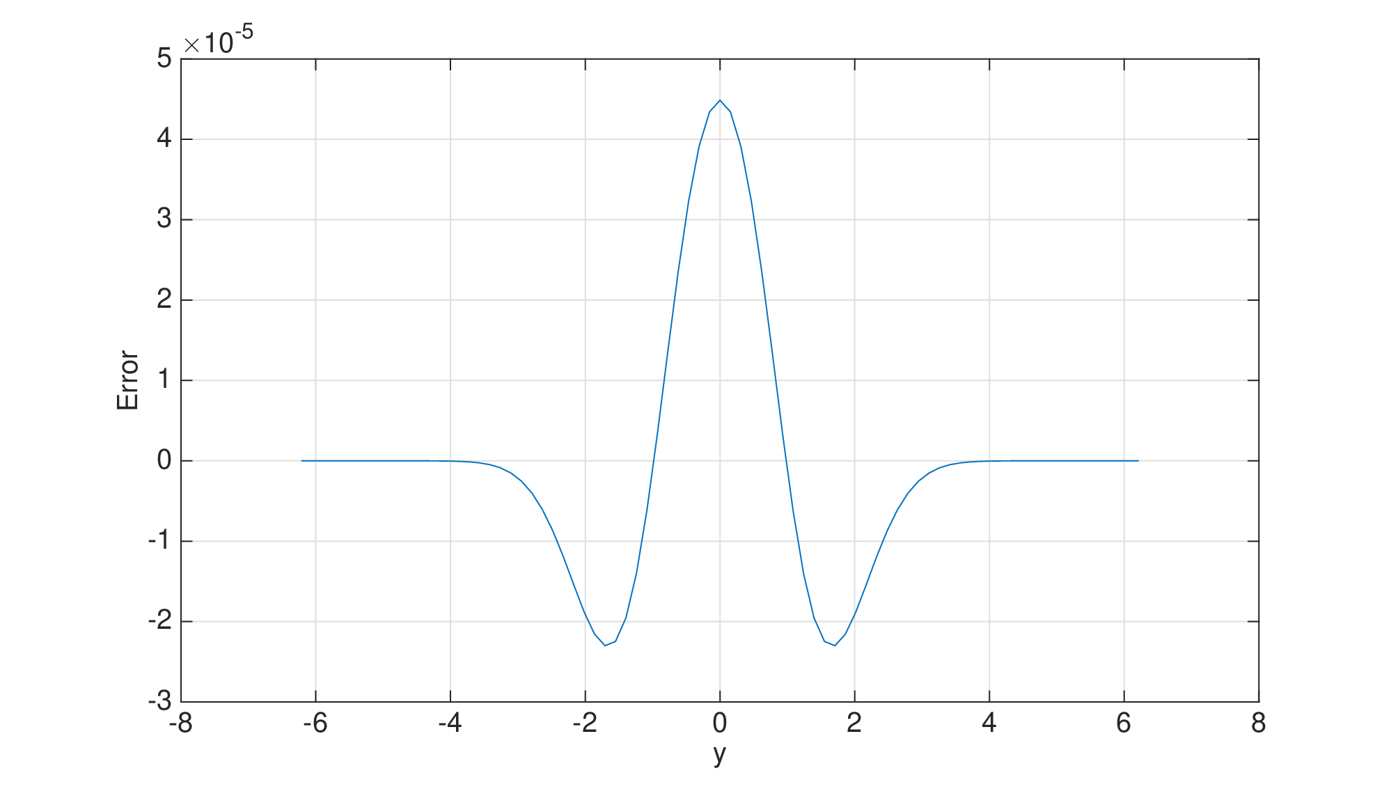
Figure 7: Toy model approximated by the discrete Fourier method and an explicit approximation for the drift term. Left, the difference between the exact and approximate solutions, with x∈[−20,20]x\in[-20,20], p∈[−20,20]p\in[-20,20], t∈[0,1]t\in[0,1], nx=1800n_{x}=1800, np=80n_{p}=80, nt=10240n_{t}=10240. Right, with the other parameters the same, the error for decreasing timestep Δ​t\Delta t with Δ​t/Δ​x2\Delta t/\Delta x^{2} held constant.
Refer to caption
Refer to caption

Finally, the right plot of Figure 7 shows the convergence rate for the solution as the grid is refined with λ=Δ​tΔ​x2\lambda=\frac{\Delta t}{\Delta x^{2}} held constant. We observe first-order convergence in time where the error is evaluated in the maximum norm. The slope of the last two points of the log-log plot is 1.00.

For this method, it is interesting to note that the maximum error in this case is approximately four times the corresponding error of the semidiscrete method (see Figures 6 and 7) and we observe upwards ‘bumps’ at around ±2\pm 2 in the latter case.

Next we present the results based on treating the drift implicitly. The left plot in Figure 8 shows the difference between the true and numerical solutions. Once again, the numerical solution itself closely resembles the result in Figure 6.

Figure 8: Toy model approximated by the discrete Fourier method with an implicit approximation for the drift term. Left, the difference between the exact and approximate solutions, with x∈[−20,20]x\in[-20,20], p∈[−20,20]p\in[-20,20], t∈[0,1]t\in[0,1], nx=1800n_{x}=1800, np=80n_{p}=80, nt=10240n_{t}=10240. Right, with the other parameters the same, the error for decreasing timestep Δ​t\Delta t with Δ​t/Δ​x2\Delta t/\Delta x^{2} held constant.
Refer to caption
Refer to caption

Finally, the right plot in Figure 8 shows the convergence rate for the solution as the grid is refined. We observe first-order convergence in time where the error is evaluated in the maximum norm. The slope of the last two points of the log-log plot is 1.00.

We observe that the maximum error in this case is approximately twice the corresponding error of the explicit drift case (see Figures 7 and 8).

5 Application to a financial hedging problem

In this section, we apply the Fourier method to a hypoelliptic problem from mathematical finance, namely the computation of hedging errors under misspecification of the market model. If the true model governing an underlying stock is known to the trader and the market is “complete”, they can perfectly hedge a position in an option by dynamic trading in the stock. If the model is unknown and the hedging strategy is based on a misspecified model, a certain profit or loss will materialize and one can ask what the distribution of this hedging error is.

Our example follows a simplified version of the analysis in El Karoui et al., [7], where the true dynamics of a single underlying asset satisfy the SDE

d​StSt=μt​d​t+σt​d​Wt,\frac{\,{\rm d}S_{t}}{S_{t}}=\mu_{t}\,{\rm d}t+\sigma_{t}\,{\rm d}W_{t}, (5.1)

where σ\sigma is a volatility process, μ\mu a drift, and WW a standard Brownian motion. We analyze the situation where the trader instead assumes that the underlying follows a different process, i.e. mis-specifies the model for SS as

d​StSt=μ^t​d​t+σ^​d​Wt\frac{\,{\rm d}S_{t}}{S_{t}}=\widehat{\mu}_{t}\,{\rm d}t+\widehat{\sigma}\,{\rm d}W_{t} (5.2)

for some constant σ^\widehat{\sigma}. We define V^​(St,t)\widehat{V}(S_{t},t) to be the (Black-Scholes) price of the European option with payoff F⁡(ST)F(S_{T}) based on the process defined in (5.2), which satisfies the PDE

ℒσ^​V^≡∂V^∂t+12​σ^2​S2​∂2V^∂S2+r​S​∂V^∂S−r​V^=0.\displaystyle\mathcal{L}^{\widehat{\sigma}}\widehat{V}\equiv\frac{\partial\widehat{V}}{\partial t}+\frac{1}{2}\widehat{\sigma}^{2}S^{2}\frac{\partial^{2}\widehat{V}}{\partial S^{2}}+rS\frac{\partial\widehat{V}}{\partial S}-r\widehat{V}=0. (5.3)

If the trader then uses the sensitivity ∂V^∂S\frac{\partial\widehat{V}}{\partial S} of V^\widehat{V} as the hedge ratio, it is shown in [7] that the hedging “error” YtY_{t}, i.e, the difference in time tt value between the option and the portfolio set up to hedge it, discounted with the risk-free rate rr to the present time, is governed by the stochastic differential equation

d​Yt=12​e−r​t​(σ^2−σt2)​St2​∂2V^∂S2​d​t.\,{\rm d}Y_{t}=\frac{1}{2}\mbox{e}^{-rt}(\widehat{\sigma}^{2}-\sigma_{t}^{2})S_{t}^{2}\frac{\partial^{2}\widehat{V}}{\partial S^{2}}\,{\rm d}t. (5.4)

We notice that the dynamics of YtY_{t} only consists of a drift term, i.e. there is no Brownian component. In the following, we assume that σt=σ\sigma_{t}=\sigma constant, but different from σ^\widehat{\sigma}.

Therefore, if we write down the Kolmogorov Forward Equation (KFE) for the probability density function PP of the pair (St,Yt)(S_{t},Y_{t}) at time tt, we find

∂P∂t\displaystyle\frac{\partial P}{\partial t} =\displaystyle= 12​σ2​∂2∂S2​(S2​P)−μ​∂∂S​(S​P)−c​∂P∂y\displaystyle\frac{1}{2}\sigma^{2}\frac{\partial^{2}}{\partial S^{2}}\left(S^{2}P\right)-\mu\frac{\partial}{\partial S}\left(SP\right)-c\frac{\partial P}{\partial y} (5.5)
=\displaystyle= 12​σ2​S2​∂2P∂S2+(2​σ2−μ)​S​∂P∂S+(σ2−μ)​P−c​∂P∂y,\displaystyle\frac{1}{2}\sigma^{2}S^{2}\frac{\partial^{2}P}{\partial S^{2}}+(2\sigma^{2}-\mu)S\frac{\partial P}{\partial S}+(\sigma^{2}-\mu)P-c\frac{\partial P}{\partial y},

where

c⁡(S,t)=12​e−r​t​(σ^2−σ2)​S2​∂2V^∂S2.\displaystyle c(S,t)=\frac{1}{2}\mbox{e}^{-rt}(\widehat{\sigma}^{2}-\sigma^{2})S^{2}\frac{\partial^{2}\widehat{V}}{\partial S^{2}}. (5.6)

The equation hence falls into the class of hypoelliptic PDEs studied in the preceding sections.

We solve the KFE numerically using the following parameters, σ=0.1\sigma=0.1, σ^=0.2\widehat{\sigma}=0.2, μ=0.05\mu=0.05, and r=0.05r=0.05. We take T=1.0T=1.0, S0=125S_{0}=125, and the option being hedged is a so-called spread with payoff defined as

F⁡(ST)=max⁡(ST−100,0)−max⁡(ST−150,0).\displaystyle F(S_{T})=\max(S_{T}-100,0)-\max(S_{T}-150,0).

We note that the convexity of this option payoff changes as SS varies, and hence also the sign of the function cc, which contains the second derivative of V^\widehat{V}. The function V^\widehat{V} is known in closed form in this case as the solution to (5.3), and so is its second derivative, referred to as the “gamma” in the financial community.

To find the univariate density of the discounted terminal hedging error, the joint density is integrated over the SS-direction. The univariate distribution of yy has been calculated using the fully-discrete Fourier method from Section 4.5. A Monte Carlo hedging simulation has been also performed where the asset price was simulated according to the true asset model (which used the true volatility) while the hedged portfolio was controlled by delta-hedging using the Black–Scholes equation with the erroneous volatility.

Figure 9 shows how the approximate distributions compare. The shape of the hedging error distribution can be rationalized by noting that the positive drift, μ\mu, implies that the stock price is more likely to move into a regime where the option gamma is negative, resulting in a preponderance of negative hedging errors. Note that in these calculations, we assume that the option is sold for a price consistent with σ^\widehat{\sigma} so that YY starts from zero. If some other price were initially realized, it would result in the densities being shifted by this amount.

For the fully-discrete Fourier method, we used S∈[5,245]S\in[5,245], y∈[−20,20]y\in[-20,20] (not plotted over whole range) and p∈[−20,20]p\in[-20,20], np=ny=220n_{p}=n_{y}=220. For the Monte Carlo results, we used 100 time steps and 100000 paths as well as 50 bins for the approximation of the density.

Figure 9: Black–Scholes model with mis-specified volatility. Comparison of the KFE solution, integrated over xx, for an increasing number of spatial steps nSn_{S} and keeping nt/nS2n_{t}/n_{S}^{2} fixed. Shown also is the empirical density from a Monte Carlo simulation as detailed in the text.
Refer to caption

Having derived an approximation to the hedging error distribution, one can compute quantities of financial interest, such as the Value-at-Risk, a quantile-based risk-measure. For instance, the 10%-quantile of the hedging error for the data set above is found to be −4.58-4.58. This compares to an initial option value of 29.31 and 26.67, respectively, for the low and high volatility.

6 Multi-dimensional problems

It is straightforward to extend the toy model (1.4), (1.5) to higher dimensions by introducing multiple diffusive terms and/or multiple drift terms. For the semidiscrete case, we expect that the analysis will be similar to that carried out for the one-dimensional case. We present this analysis in the remainder of this section.

6.1 Multiple diffusive terms

We consider the case of a PDE with a single drift coefficient which is a linear combination of the components of xx,

∂u∂t+(γ1​x1+γ2​x2)​∂u∂y\displaystyle\frac{\partial u}{\partial t}+(\gamma_{1}x_{1}+\gamma_{2}x_{2})\frac{\partial u}{\partial y} =a11​∂2u∂x12+2​a12​∂2u∂x1​∂x2+a22​∂2u∂x22,\displaystyle=a_{11}\frac{\partial^{2}u}{\partial x_{1}^{2}}+2a_{12}\frac{\partial^{2}u}{\partial x_{1}\partial x_{2}}+a_{22}\frac{\partial^{2}u}{\partial x_{2}^{2}}, (x1,x2,y,t)∈ℝ3×(0,T],\displaystyle\quad(x_{1},x_{2},y,t)\in\mathbb{R}^{3}\times(0,T], (6.1)
u⁡(x1,x2,y,0)\displaystyle u(x_{1},x_{2},y,0) =δ⁡(x1−x1,0)⊗δ⁡(x2−x2,0)⊗δ⁡(y−y0),\displaystyle=\delta(x_{1}-x_{1,0})\otimes\delta(x_{2}-x_{2,0})\otimes\delta(y-y_{0}), (x1,x2,y)∈ℝ3,\displaystyle\quad(x_{1},x_{2},y)\in\mathbb{R}^{3},

which extends the toy model to one containing two independent variables x1x_{1} and x2x_{2}. We consider the hypoelliptic case, i.e., where (γ1,γ2)≠(0,0)(\gamma_{1},\gamma_{2})\neq(0,0) and (ai​j)1≤i,j,≤2(a_{ij})_{1\leq i,j,\leq 2} is strictly positive definite, i.e., a11,a22>0a_{11},a_{22}>0 and a11​a22>a122a_{11}a_{22}>a_{12}^{2}.

We apply the yy-FT to get

∂v∂t−i​p​(γ1​x1+γ2​x2)​v=a11​∂2v∂x12+2​a12​∂2v∂x1​∂x2+a22​∂2v∂x22,(x1,x2,p,t)∈ℝ3×(0,T].\displaystyle\frac{\partial v}{\partial t}-ip(\gamma_{1}x_{1}+\gamma_{2}x_{2})v=a_{11}\frac{\partial^{2}v}{\partial x_{1}^{2}}+2a_{12}\frac{\partial^{2}v}{\partial x_{1}\partial x_{2}}+a_{22}\frac{\partial^{2}v}{\partial x_{2}^{2}},\quad(x_{1},x_{2},p,t)\in\mathbb{R}^{3}\times(0,T]. (6.2)

Now for the analytical solution we next apply the x1x_{1}-FT and the x2x_{2}-FT in turn to get

∂w∂t−p⁡(γ1​∂w∂s1+γ2​∂w∂s2)=−(a11​s12+2​a12​s1​s2+a22​s22)​w,(s1,s2,p,t)∈ℝ3×(0,T],\displaystyle\frac{\partial w}{\partial t}-p\bigg(\gamma_{1}\frac{\partial w}{\partial s_{1}}+\gamma_{2}\frac{\partial w}{\partial s_{2}}\bigg)=-(a_{11}s_{1}^{2}+2a_{12}s_{1}s_{2}+a_{22}s_{2}^{2})w,\quad(s_{1},s_{2},p,t)\in\mathbb{R}^{3}\times(0,T], (6.3)

in conjunction with the initial condition

w⁡(s1,s2,p,0)=1.w(s_{1},s_{2},p,0)=1.

We can now solve this first-order hyperbolic initial-value problem directly, but we can also use an ansatz by seeking a solution of the form

w⁡(s1,s2,p,t)=exp⁡(−a11​s12​t−2​a12​s1​s2​t−a22​s22​t​x​s−B1​s1​p​t2−B2​s2​p​t2−C​p2​t3)w(s_{1},s_{2},p,t)=\exp{(-a_{11}s_{1}^{2}t-2a_{12}s_{1}s_{2}t-a_{22}s_{2}^{2}txs-B_{1}s_{1}pt^{2}-B_{2}s_{2}pt^{2}-Cp^{2}t^{3})}

and then finding the coefficients that fit the PDE. By insertion we get

B1\displaystyle B_{1} =γ1​a11+γ2​a12,\displaystyle=\gamma_{1}a_{11}+\gamma_{2}a_{12},
B2\displaystyle B_{2} =γ1​a12+γ2​a22,\displaystyle=\gamma_{1}a_{12}+\gamma_{2}a_{22},
C\displaystyle C =13​(γ1​(a11+a12)+γ2​(a12+a22)),\displaystyle=\frac{1}{3}(\gamma_{1}(a_{11}+a_{12})+\gamma_{2}(a_{12}+a_{22})),

and thus we have the analytical solution in Fourier space. We could, if necessary, invert all these transforms but we will instead concentrate on the effect of discretization in the x1x_{1}- and x2x_{2}-directions. So we now start with the PDE (6.2) and discretize this as follows by writing

∂Vj,k∂t−i​p​(γ1​x1,j+γ2​x2,k)​Vj,k\displaystyle\frac{\partial V_{j,k}}{\partial t}-ip(\gamma_{1}x_{1,j}+\gamma_{2}x_{2,k})V_{j,k} =\displaystyle= a11​Vj+1,k−2​Vj,k+Vj−1,kΔ​x12+a22​Vj,k+1−2​Vj,k+Vj,k−1Δ​x22\displaystyle a_{11}\frac{V_{j+1,k}-2V_{j,k}+V_{j-1,k}}{\Delta x_{1}^{2}}+\,a_{22}\frac{V_{j,k+1}-2V_{j,k}+V_{j,k-1}}{\Delta x_{2}^{2}}
+ 2​a12​Vj+1,k+1−Vj+1,k−1−Vj−1,k+1+Vj−1,k−14​Δ​x1​Δ​x2,\displaystyle\qquad+\,2a_{12}\frac{V_{j+1,k+1}-V_{j+1,k-1}-V_{j-1,k+1}+V_{j-1,k-1}}{4\Delta x_{1}\Delta x_{2}},

where we have omitted pp and tt as arguments for the sake of brevity, and where Vj,k​(p,t)V_{j,k}(p,t) is an approximation to v⁡(x1,j,x2,k,p,t)v(x_{1,j},x_{2,k},p,t) on a uniform two-dimensional mesh of widths Δ​x1,Δ​x2>0\Delta x_{1},\Delta x_{2}>0. We can then apply the Fourier transforms in the x1x_{1} and x2x_{2} variables and after steps similar to the one-dimensional case obtain the solution for the double-transformed equation,

W⁡(s1,s2,p,t)=w⁡(s1,s2,p,t)​exp⁡(1p​∫s1s1+p​t(a11​g11​(σ,s2)+2​a12​g12​(σ,s2)+a22​g22​(σ,s2))​𝑑σ),W(s_{1},s_{2},p,t)=w(s_{1},s_{2},p,t)\exp{\bigg(\frac{1}{p}\int^{s_{1}+pt}_{s_{1}}(a_{11}g_{11}(\sigma,s_{2})+2a_{12}g_{12}(\sigma,s_{2})+a_{22}g_{22}(\sigma,s_{2}))\,{\rm d}\sigma\bigg)}, (6.4)

where

g11​(s1,s2)\displaystyle g_{11}(s_{1},s_{2}) =s12−4Δ​x12​sin2⁡(s1​Δ​x12),\displaystyle=s_{1}^{2}-\frac{4}{\Delta x_{1}^{2}}\sin^{2}{\bigg(\frac{s_{1}\Delta x_{1}}{2}\bigg)},
g12​(s1,s2)\displaystyle g_{12}(s_{1},s_{2}) =s1​s2−1Δ​x1​Δ​x2​sin⁡(s1​Δ​x1)​sin⁡(s2​Δ​x2),\displaystyle=s_{1}s_{2}-\frac{1}{\Delta x_{1}\Delta x_{2}}\sin{(s_{1}\Delta x_{1})}\sin{(s_{2}\Delta x_{2})},
g22​(s1,s2)\displaystyle g_{22}(s_{1},s_{2}) =s22−4Δ​x22​sin2⁡(s2​Δ​x22).\displaystyle=s_{2}^{2}-\frac{4}{\Delta x_{2}^{2}}\sin^{2}{\bigg(\frac{s_{2}\Delta x_{2}}{2}\bigg)}.

We can now investigate the low and high wavenumber behaviour in terms of the new variables. For the sake of simplicity of the exposition, we shall do this for the special case γ1=1\gamma_{1}=1, γ2=0\gamma_{2}=0, a11=a22=1a_{11}=a_{22}=1, a12=ρ∈(−1,1)a_{12}=\rho\in(-1,1), i.e., we consider

∂u∂t+x1​∂u∂y=∂2u∂x12+2​ρ​∂2u∂x1​∂x2+∂2u∂x22.\displaystyle\frac{\partial u}{\partial t}+x_{1}\frac{\partial u}{\partial y}=\frac{\partial^{2}u}{\partial x_{1}^{2}}+2\rho\frac{\partial^{2}u}{\partial x_{1}\partial x_{2}}+\frac{\partial^{2}u}{\partial x_{2}^{2}}. (6.5)
Remark 4.

Equation (6.5) is a simplified case of the general equation (6.1), where the term x2x_{2} has been dropped from the drift and the diffusion is normalized. This can be achieved by a rotation of the original co-ordinates to align the drift (γ1,γ2)(\gamma_{1},\gamma_{2}) with the x1x_{1}-axis, and by subsequent scaling of the new yy, x1x_{1} and x2x_{2} co-ordinates.

In this case, the numerical solution is

W⁡(s1,s2,p,t)=w⁡(s1,s2,p,t)​exp⁡(1p​∫s1s1+p​t(g11​(σ,s2)+2​ρ​g12​(σ,s2)+g22​(σ,s2))​𝑑σ).\displaystyle W(s_{1},s_{2},p,t)=w(s_{1},s_{2},p,t)\exp{\bigg(\frac{1}{p}\int^{s_{1}+pt}_{s_{1}}(g_{11}(\sigma,s_{2})+2\rho g_{12}(\sigma,s_{2})+g_{22}(\sigma,s_{2}))\,{\rm d}\sigma\bigg)}.

Similarly to the one-dimensional case, this leads us to investigate

W(s1,s2,p,t)=W1(s1,p,t)exp(−1p∫s1s1+p​t(2ρsin⁡(σ​Δ​x1)​sin⁡(s2​Δ​x2)Δ​x1​Δ​x2+4Δ​x22sin2(s2​Δ​x22))dσ),W(s_{1},s_{2},p,t)=W_{1}(s_{1},p,t)\ \exp\bigg(-\frac{1}{p}\int^{s_{1}+pt}_{s_{1}}\left(2\rho\frac{\sin{(\sigma\Delta x_{1})}\sin{(s_{2}\Delta x_{2})}}{\Delta x_{1}\Delta x_{2}}+\frac{4}{\Delta x_{2}^{2}}\sin^{2}{\bigg(\frac{s_{2}\Delta x_{2}}{2}\bigg)}\right)\,{\rm d}\sigma\bigg),

where W1W_{1} is the solution from the one-dimensional case. By standard integration and the change of variables ξ=p​t/2\xi=pt/2 and η1=s1+p​t/2\eta_{1}=s_{1}+pt/2 we find this to be

W⁡(η1,s2,ξ,t)=W1​(η1,ξ,t)​exp⁡(−2​t​ρ​sinc⁡(ξ​Δ​x1)​sin⁡(η1​Δ​x1)Δ​x1​sin⁡(s2​Δ​x2)Δ​x2−4​tΔ​x22​sin2⁡(s2​Δ​x2/2)),\displaystyle W(\eta_{1},s_{2},\xi,t)=W_{1}(\eta_{1},\xi,t)\,\exp\bigg(-2t\rho\sinc(\xi\Delta x_{1})\frac{\sin(\eta_{1}\Delta x_{1})}{\Delta x_{1}}\frac{\sin(s_{2}\Delta x_{2})}{\Delta x_{2}}-\frac{4t}{\Delta x_{2}^{2}}\sin^{2}(s_{2}\Delta x_{2}/2)\bigg),

where

W1​(η1,ξ,t)=exp⁡(−2​tΔ​x12​(1−sinc⁡(ξ​Δ​x1)​cos⁡(η1​Δ​x1))).\displaystyle W_{1}(\eta_{1},\xi,t)=\exp\bigg(-\frac{2t}{\Delta x_{1}^{2}}\left(1-\sinc(\xi\Delta x_{1})\cos(\eta_{1}\Delta x_{1})\right)\bigg).

The exact solution in these variables is

w⁡(η1,s2,ξ,t)=exp⁡(−t⁡{η12+ξ23+s22+2​ρ​η1​s2})\displaystyle w(\eta_{1},s_{2},\xi,t)=\exp{\left(-t\left\{\eta_{1}^{2}+\frac{\xi^{2}}{3}+s_{2}^{2}+2\rho\eta_{1}s_{2}\right\}\right)} (6.6)

and we recognize in the first two terms the one-dimensional solution

w1​(η1,ξ,t)=exp⁡(−t⁡{η12+ξ23}).\displaystyle w_{1}(\eta_{1},\xi,t)=\exp{\left(-t\left\{\eta_{1}^{2}+\frac{\xi^{2}}{3}\right\}\right)}. (6.7)

We proceed by a wavenumber analysis broadly similar to the one before, but made somewhat more complicated by the presence of an extra variable s2s_{2} and the fact that the problem degenerates as |ρ|→1|\rho|\rightarrow 1, necessitating a more careful estimation for ρ\rho close to 1.

6.2 Joint low wavenumbers

We write

log⁡W=log⁡W1−t⁡{2​ρ​sinc⁡(ξ​Δ​x1)​sin⁡(η1​Δ​x1)Δ​x1​sin⁡(s2​Δ​x2)Δ​x2+4Δ​x22​sin2⁡(s2​Δ​x22)}\displaystyle\log W=\log W_{1}-t\left\{2\rho\sinc(\xi\Delta x_{1})\frac{\sin(\eta_{1}\Delta x_{1})}{\Delta x_{1}}\frac{\sin\left(s_{2}\Delta x_{2}\right)}{\Delta x_{2}}+\frac{4}{\Delta x_{2}^{2}}\sin^{2}\left(\frac{s_{2}\Delta x_{2}}{2}\right)\right\}

and compare this to

log⁡w=log⁡w1−t⁡{s22+2​ρ​η1​s2},\displaystyle\log w=\log w_{1}-t\{s_{2}^{2}+2\rho\eta_{1}s_{2}\},

where ww is the exact solution to the two-dimensional problem from (6.6) and w1w_{1} is the solution to the one-dimensional problem from (6.7). By standard Taylor expansion we find

log⁡(W/w)\displaystyle\log(W/w) =log⁡(W1/w1)+2​ρ​t​(112​η1​s23​Δ​x22+16​η13​s22​Δ​x12+η1​s22​ξ2​Δ​x12)+t12​s24​Δ​x22+o⁡(Δ​x12)+o⁡(Δ​x22)\displaystyle=\log(W_{1}/w_{1})+2\rho t\left(\frac{1}{12}\eta_{1}s_{2}^{3}\Delta x_{2}^{2}+\frac{1}{6}\eta_{1}^{3}s_{2}^{2}\Delta x_{1}^{2}+\eta_{1}s_{2}^{2}\xi^{2}\Delta x_{1}^{2}\right)+\frac{t}{12}s_{2}^{4}\Delta x_{2}^{2}+o(\Delta x_{1}^{2})+o(\Delta x_{2}^{2})
=log⁡(W1/w1)+(ρ​t3​η13​s22+2​ρ​t​η1​s22​ξ2)​Δ​x12+(ρ​t6​η1​s23+t12​s24)​Δ​x22+o⁡(Δ​x12)+o⁡(Δ​x22)\displaystyle=\log(W_{1}/w_{1})+\left(\frac{\rho t}{3}\eta_{1}^{3}s_{2}^{2}+2\rho t\eta_{1}s_{2}^{2}\xi^{2}\right)\Delta x_{1}^{2}+\left(\frac{\rho t}{6}\eta_{1}s_{2}^{3}+\frac{t}{12}s_{2}^{4}\right)\Delta x_{2}^{2}+o(\Delta x_{1}^{2})+o(\Delta x_{2}^{2})
=(2​t4!​η14+2​t5!​ξ4+ρ​t3​η13​s22+2​ρ​t​η1​s22​ξ2)​Δ​x12+(ρ​t6​η1​s23+t12​s24)​Δ​x22+o⁡(Δ​x12)+o⁡(Δ​x22).\displaystyle=\left(\frac{2t}{4!}\eta_{1}^{4}+\frac{2t}{5!}\xi^{4}+\frac{\rho t}{3}\eta_{1}^{3}s_{2}^{2}+2\rho t\eta_{1}s_{2}^{2}\xi^{2}\right)\Delta x_{1}^{2}+\left(\frac{\rho t}{6}\eta_{1}s_{2}^{3}+\frac{t}{12}s_{2}^{4}\right)\Delta x_{2}^{2}+o(\Delta x_{1}^{2})+o(\Delta x_{2}^{2}).

Therefore the numerical error contribution from the low wavenumber regime is

I1​(x1,x2,y,t)\displaystyle I_{1}(x_{1},x_{2},y,t) =Δ​x12​F1​(x1,x2,y,t)+Δ​x22​F2​(x1,x2,y,t)+o⁡(Δ​x12)+o⁡(Δ​x22),\displaystyle=\Delta x_{1}^{2}F_{1}(x_{1},x_{2},y,t)+\Delta x_{2}^{2}F_{2}(x_{1},x_{2},y,t)+o(\Delta x_{1}^{2})+o(\Delta x_{2}^{2}), (6.8)

where

F1\displaystyle F_{1} =t2​(14!​(∂∂x1+t2​∂∂y)4+15!​(t2​∂∂y)4)​u\displaystyle=t^{2}\left(\frac{1}{4!}\left(\frac{\partial}{\partial x_{1}}+\frac{t}{2}\frac{\partial}{\partial y}\right)^{4}+\frac{1}{5!}\left(\frac{t}{2}\frac{\partial}{\partial y}\right)^{4}\right)\ u
+t2​(ρ3!​(∂∂x1+t2​∂∂y)3​∂2∂x22+ρ⁡(∂∂x1+t2​∂∂y)​∂2∂x22​(t2​∂∂y)2)​u\displaystyle\hskip 56.9055pt+\ t^{2}\left(\frac{\rho}{3!}\left(\frac{\partial}{\partial x_{1}}+\frac{t}{2}\frac{\partial}{\partial y}\right)^{3}\frac{\partial^{2}}{\partial x_{2}^{2}}+\rho\left(\frac{\partial}{\partial x_{1}}+\frac{t}{2}\frac{\partial}{\partial y}\right)\frac{\partial^{2}}{\partial x_{2}^{2}}\left(\frac{t}{2}\frac{\partial}{\partial y}\right)^{2}\right)\ u
F2\displaystyle F_{2} =t2​(2​ρ4!​(∂∂x1+t2​∂∂y)​∂3∂x23+14!​∂4∂x24)​u.\displaystyle=t^{2}\left(\frac{2\rho}{4!}\left(\frac{\partial}{\partial x_{1}}+\frac{t}{2}\frac{\partial}{\partial y}\right)\frac{\partial^{3}}{\partial x_{2}^{3}}+\frac{1}{4!}\frac{\partial^{4}}{\partial x_{2}^{4}}\right)\ u.

The point is less the explicit form, but that the error can be expressed in terms of up to fifth mixed partial derivatives, or up to fourth if ρ=0\rho=0. As in Section 3, we will find that this is the only wavenumber range that contributes to the leading order error, and therefore, up to higher order terms, (6.8) fully describes the discretization error.

6.3 Low 𝝃\boldsymbol{\xi}-wavenumbers and high 𝜼𝟏\boldsymbol{\eta_{1}}- or 𝐬𝟐\bf s_{2}-wavenumbers

We require two simple inequalities. The first one states that for |η1​Δ​x1|≤π/2|\eta_{1}\Delta x_{1}|\leq\pi/2, and since sinc⁡(ξ​Δ​x1)>0\sinc(\xi\Delta x_{1})>0 (in the present small ξ\xi regime),

1−sinc⁡(ξ​Δ​x1)​cos⁡(η1​Δ​x1)≥1−cos⁡(η1​Δ​x1)=2​sin2⁡(η1​Δ​x1/2).1-\sinc(\xi\Delta x_{1})\cos(\eta_{1}\Delta x_{1})\geq 1-\cos(\eta_{1}\Delta x_{1})=2\sin^{2}(\eta_{1}\Delta x_{1}/2).

The second elementary inequality used in the argument below, in the transition from the second-to-last inequality to the last inequality, is that

sin⁡α≥2π​αfor0≤α≤π2.\sin\alpha\geq\frac{2}{\pi}\alpha\qquad\mbox{for}\qquad 0\leq\alpha\leq\frac{\pi}{2}.

Therefore

W⁡(η1,s2)\displaystyle W(\eta_{1},s_{2}) ≤exp⁡(−4​tΔ​x12​sin2⁡(η1​Δ​x1/2)+2​t​|ρ|​|sin⁡(η1​Δ​x1)|Δ​x1​|sin⁡(s2​Δ​x2)|Δ​x2−4​tΔ​x22​sin2⁡(s2​Δ​x2/2))\displaystyle\leq\exp\bigg(-\frac{4t}{\Delta x_{1}^{2}}\sin^{2}(\eta_{1}\Delta x_{1}/2)+2t|\rho|\frac{|\sin(\eta_{1}\Delta x_{1})|}{\Delta x_{1}}\frac{|\sin(s_{2}\Delta x_{2})|}{\Delta x_{2}}-\frac{4t}{\Delta x_{2}^{2}}\sin^{2}(s_{2}\Delta x_{2}/2)\bigg)
≤exp⁡(−4​tΔ​x12​sin2⁡(η1​Δ​x1/2)+8​t​|ρ|​|sin⁡(η1​Δ​x1/2)|Δ​x1​|sin⁡(s2​Δ​x2/2)|Δ​x2−4​tΔ​x22​sin2⁡(s2​Δ​x2/2))\displaystyle\leq\exp\bigg(-\frac{4t}{\Delta x_{1}^{2}}\sin^{2}(\eta_{1}\Delta x_{1}/2)+8t|\rho|\frac{|\sin(\eta_{1}\Delta x_{1}/2)|}{\Delta x_{1}}\frac{|\sin(s_{2}\Delta x_{2}/2)|}{\Delta x_{2}}-\frac{4t}{\Delta x_{2}^{2}}\sin^{2}(s_{2}\Delta x_{2}/2)\bigg)
=exp⁡(−4​t​(1−|ρ|)​(1Δ​x12​sin2⁡(η1​Δ​x1/2)+1Δ​x22​sin2⁡(s2​Δ​x2/2)))\displaystyle=\exp\bigg(-4t(1-|\rho|)\left(\frac{1}{\Delta x_{1}^{2}}\sin^{2}(\eta_{1}\Delta x_{1}/2)+\frac{1}{\Delta x_{2}^{2}}\sin^{2}(s_{2}\Delta x_{2}/2)\right)\bigg)
⋅exp⁡(−4​t​|ρ|​(sin⁡(η1​Δ​x1/2)Δ​x1−sin2⁡(s2​Δ​x2)Δ​x2)2)\displaystyle\hskip 142.26378pt\cdot\;\exp\bigg(-4t|\rho|\left(\frac{\sin(\eta_{1}\Delta x_{1}/2)}{\Delta x_{1}}-\frac{\sin^{2}(s_{2}\Delta x_{2})}{\Delta x_{2}}\right)^{2}\bigg)
≤exp⁡(−4​t​(1−|ρ|)​(1Δ​x12​sin2⁡(η1​Δ​x1/2)+1Δ​x22​sin2⁡(s2​Δ​x2/2)))\displaystyle\leq\exp\bigg(-4t(1-|\rho|)\left(\frac{1}{\Delta x_{1}^{2}}\sin^{2}(\eta_{1}\Delta x_{1}/2)+\frac{1}{\Delta x_{2}^{2}}\sin^{2}(s_{2}\Delta x_{2}/2)\right)\bigg)
≤exp⁡(−4​t​(1−|ρ|)π2​(η12+s22))\displaystyle\leq\exp\bigg(-\frac{4\,t\,(1-|\rho|)}{\pi^{2}}\left(\eta_{1}^{2}+s_{2}^{2}\right)\bigg)
=o(Δxr)as Δ​x→0\displaystyle=o(\Delta x^{r})\qquad\mbox{as $\Delta x\rightarrow 0$}

for any r>0r>0 if either ν1≥Δ​x1−q\nu_{1}\geq\Delta x_{1}^{-q} or s2≥Δ​x2−qs_{2}\geq\Delta x_{2}^{-q} for any q>0q>0.

For |η1​Δ​x1|>π/2|\eta_{1}\Delta x_{1}|>\pi/2, we have that

1−sinc⁡(ξ​Δ​x1)​cos⁡(η1​Δ​x1)≥1,1-\sinc(\xi\Delta x_{1})\cos(\eta_{1}\Delta x_{1})\geq 1,

and therefore

W⁡(η1,s2)\displaystyle W(\eta_{1},s_{2}) ≤exp⁡(−2​tΔ​x12+2​t​|ρ|​1Δ​x1​|sin⁡(s2​Δ​x2)|Δ​x2−4​tΔ​x22​sin2⁡(s2​Δ​x2/2))\displaystyle\leq\exp\bigg(-\frac{2t}{\Delta x_{1}^{2}}+2t|\rho|\frac{1}{\Delta x_{1}}\frac{|\sin(s_{2}\Delta x_{2})|}{\Delta x_{2}}-\frac{4t}{\Delta x_{2}^{2}}\sin^{2}(s_{2}\Delta x_{2}/2)\bigg)
≤exp⁡(−2​tΔ​x12+4​tΔ​x1​|sin⁡(s2​Δ​x2/2)|Δ​x2−4​tΔ​x22​sin2⁡(s2​Δ​x2/2))\displaystyle\leq\exp\bigg(-\frac{2t}{\Delta x_{1}^{2}}+\frac{4t}{\Delta x_{1}}\frac{|\sin(s_{2}\Delta x_{2}/2)|}{\Delta x_{2}}-\frac{4t}{\Delta x_{2}^{2}}\sin^{2}(s_{2}\Delta x_{2}/2)\bigg)
≤exp⁡(−2​tΔ​x12+21​tΔ​x1​|sin⁡(s2​Δ​x2/2)|Δ​x2−4​tΔ​x22​sin2⁡(s2​Δ​x2/2))\displaystyle\leq\exp\bigg(-\frac{2t}{\Delta x_{1}^{2}}+\frac{\sqrt{21}t}{\Delta x_{1}}\frac{|\sin(s_{2}\Delta x_{2}/2)|}{\Delta x_{2}}-\frac{4t}{\Delta x_{2}^{2}}\sin^{2}(s_{2}\Delta x_{2}/2)\bigg)
=exp(−t2(1Δ​x12+1Δ​x22sin2(s2Δx2/2)))⋅\displaystyle=\exp\bigg(-\frac{t}{2}\left(\frac{1}{\Delta x_{1}^{2}}+\frac{1}{\Delta x_{2}^{2}}\sin^{2}(s_{2}\Delta x_{2}/2)\right)\bigg)\cdot
⋅exp⁡(−t​(32​1Δ​x1−72​|sin⁡(s2​Δ​x2/2)|Δ​x2)2)\displaystyle\hskip 142.26378pt\cdot\;\exp\bigg(-t\left(\sqrt{\frac{3}{2}}\frac{1}{\Delta x_{1}}-\sqrt{\frac{7}{2}}\frac{|\sin(s_{2}\Delta x_{2}/2)|}{\Delta x_{2}}\right)^{2}\bigg)
≤exp⁡(−t2​(1Δ​x12+1Δ​x22​sin2⁡(s2​Δ​x2/2)))\displaystyle\leq\exp\bigg(-\frac{t}{2}\left(\frac{1}{\Delta x_{1}^{2}}+\frac{1}{\Delta x_{2}^{2}}\sin^{2}(s_{2}\Delta x_{2}/2)\right)\bigg)
=o⁡(Δ​xr)\displaystyle=o(\Delta x^{r})

as before.

6.4 High 𝝃\boldsymbol{\xi}-wavenumbers

Completing squares, we write

W⁡(η1,s2,ξ)\displaystyle W(\eta_{1},s_{2},\xi) =W1(η1,ξ)⋅exp(tΔ​x12cos2(s2Δx2/2)sinc2(ξΔx1)sin2(η1Δx1)ρ2)⋅\displaystyle=W_{1}(\eta_{1},\xi)\,\cdot\,\exp\left(\frac{t}{\Delta x_{1}^{2}}\cos^{2}(s_{2}\Delta x_{2}/2)\sinc^{2}(\xi\Delta x_{1})\sin^{2}(\eta_{1}\Delta x_{1})\rho^{2}\right)\,\cdot
⋅exp⁡(−t​(ρΔ​x1​cos⁡(s2​Δ​x2/2)​sinc⁡(ξ​Δ​x1)​sin⁡(η1​Δ​x1)+2Δ​x2​sin⁡(s2​Δ​x2/2))2),\displaystyle\qquad\cdot\,\exp\left(-t\left(\frac{\rho}{\Delta x_{1}}\cos(s_{2}\Delta x_{2}/2)\sinc(\xi\Delta x_{1})\sin(\eta_{1}\Delta x_{1})+\frac{2}{\Delta x_{2}}\sin(s_{2}\Delta x_{2}/2)\right)^{2}\right),

and so, neglecting the last factor, which is ≤1\leq 1,

log⁡W\displaystyle\log W ≤−2​tΔ​x12​(1−sinc⁡(ξ​Δ​x1)​cos⁡(η1​Δ​x1))+ρ2​tΔ​x12​cos2⁡(s2​Δ​x2/2)​sinc2⁡(ξ​Δ​x1)​sin2⁡(η1​Δ​x1)\displaystyle\leq-\frac{2t}{\Delta x_{1}^{2}}\left(1-\sinc(\xi\Delta x_{1})\cos(\eta_{1}\Delta x_{1})\right)+\rho^{2}\frac{t}{\Delta x_{1}^{2}}\cos^{2}(s_{2}\Delta x_{2}/2)\sinc^{2}(\xi\Delta x_{1})\sin^{2}(\eta_{1}\Delta x_{1})
≤tΔ​x12​(−2+2​sinc⁡(ξ​Δ​x1)​cos⁡(η1​Δ​x1)+sinc2⁡(ξ​Δ​x1)​sin2⁡(η1​Δ​x1))\displaystyle\leq\frac{t}{\Delta x_{1}^{2}}\left(-2+2\sinc(\xi\Delta x_{1})\cos(\eta_{1}\Delta x_{1})+\sinc^{2}(\xi\Delta x_{1})\sin^{2}(\eta_{1}\Delta x_{1})\right)
≤tΔ​x12​(−2+|sinc⁡(ξ​Δ​x1)|​(2​|cos⁡(η1​Δ​x1)|+sin2⁡(η1​Δ​x1)))\displaystyle\leq\frac{t}{\Delta x_{1}^{2}}\left(-2+|\sinc(\xi\Delta x_{1})|\left(2|\cos(\eta_{1}\Delta x_{1})|+\sin^{2}(\eta_{1}\Delta x_{1})\right)\right)
=tΔ​x12​(−2+|sinc⁡(ξ​Δ​x1)|​(2−(1−|cos⁡(η1​Δ​x1)|)2))\displaystyle=\frac{t}{\Delta x_{1}^{2}}\left(-2+|\sinc(\xi\Delta x_{1})|\left(2-(1-|\cos(\eta_{1}\Delta x_{1})|)^{2}\right)\right)
≤−2​tΔ​x12​(1−|sinc⁡(ξ​Δ​x1)|),\displaystyle\leq-\frac{2t}{\Delta x_{1}^{2}}(1-|\sinc(\xi\Delta x_{1})|),

and following the remainder of the argument in the one-dimensional case we can deduce that the contribution from this range is also exponentially small.

6.5 Multiple drift terms

Another possible extension is a model of the form

∂u∂t+a1​x​∂u∂y1+a2​x​∂u∂y2=∂2u∂x2,\frac{\partial u}{\partial t}+a_{1}x\frac{\partial u}{\partial y_{1}}+a_{2}x\frac{\partial u}{\partial y_{2}}=\frac{\partial^{2}u}{\partial x^{2}}, (6.9)

where (a1,a2)≠(0,0)(a_{1},a_{2})\neq(0,0) so that we have two drift terms and neither of the drift coefficients depend on yy. For this, we can apply the y1y_{1}-FT and the y2y_{2}-FT to get

∂v∂t−i​a1​p1​x​v−i​a2​p2​x​v=∂2v∂x2,\frac{\partial v}{\partial t}-ia_{1}p_{1}xv-ia_{2}p_{2}xv=\frac{\partial^{2}v}{\partial x^{2}},

where p1p_{1} and p2p_{2} are wavenumbers. To find the analytical solution we apply the xx-FT to get

∂w∂t−(a1​p1+a2​p2)​∂w∂s=−s2​w.\frac{\partial w}{\partial t}-(a_{1}p_{1}+a_{2}p_{2})\frac{\partial w}{\partial s}=-s^{2}w.

The analysis would then continue as before but with a1​p1+a2​p2a_{1}p_{1}+a_{2}p_{2} as a joint wavenumber. In this situation however the wavenumbers have to be handled differently. For example, we can have separately large values of |p1||p_{1}| and |p2||p_{2}| but the value of a1​p1+a2​p2a_{1}p_{1}+a_{2}p_{2} can be small.

7 Conclusions

The numerical analysis of hypoelliptic PDEs with variable coefficients and Dirac initial datum is notoriously difficult because standard approaches to convergence analysis are not directly applicable. In contrast with parabolic initial-value problems, in the case of hypoelliptic PDEs the situation is complicated by the fact that diffusion generally acts only in some, but not all, co-ordinate directions. The approach of [1] for the one-dimensional heat equation is based on Fourier analysis to show approximation of a certain order for the low wavenumber components and exponential decay of the high wavenumber components for smoothing schemes. In the present case of hypoelliptic equations the analysis is more intricate because of the interplay of wavenumbers in the different co-ordinate directions as a consequence of variable coefficients and the resulting noncommutativity of the spatial differential operators in the different directions.

We exploit the special structure of the Kolmogorov equations under consideration by performing a Fourier transform in the direction with the pure transport term, and discretize in the diffusive direction(s) by a finite difference scheme. This results in a parametrized system of semi-discrete equations, which can be solved by standard methods, and the resulting solution is then transformed back from Fourier space using exponentially convergent numerical quadrature, thus leading to an effective technique for dimensional reduction. The numerical analysis sheds light on the interaction of different wavenumbers and allows us to derive second-order convergence for the proposed numerical scheme in the absence of time-discretization.

An open question at present is how to replicate the analysis herein for the fully discrete counterpart of the method, which also includes time-discretization. Although unconditional stability of the backward Euler scheme for initial data in L2L^{2}, can be proved by standard energy estimates, a similar argument does not seem to apply in the case of Dirac initial datum, as the use of a discrete negative-order Sobolev norm, which would be the natural choice of norm for the discrete representation of the Dirac function on the finite difference grid, in conjunction with discrete counterparts of parabolic smoothing estimates in the diffusive directions, is obstructed by the particular form of the variable coefficients in the Kolmogorov equations under consideration, and the complex nature of error propagation for the fully-discrete scheme has not so far allowed a rigorous convergence analysis of the fully discrete scheme.

References

  • [1] R. Carter and M. B. Giles. Sharp error estimates for discretizations of the 1D convection-diffusion equation with Dirac initial data. IMA Journal of Numerical Analysis, 27(2):406–425, 2007.
  • [2] E. L. Foster, J. Lohéac, and M.-B. Tran. A structure preserving scheme for the Kolmogorov-Fokker-Planck equation. arXiv preprint arXiv:1411.1019, 2014.
  • [3] M. B. Giles. Sharp error estimates for a discretisation of the 1D convection-diffusion equation with Dirac initial data. Technical Report 04-17, Oxford University Computing Laboratory, https://people.maths.ox.ac.uk/gilesm/files/NA-04-17.pdf, 2004.
  • [4] N. J. Higham. The scaling and squaring method for the matrix exponential revisited. SIAM Journal on Matrix Analysis and Applications, 26(4):1179–1193, 2005.
  • [5] L. Hörmander. Hypoelliptic second order differential equations. Acta Mathematica, 119(1):147–171, 1967.
  • [6] B. S. Jovanović and E. Süli. Analysis of finite difference schemes for linear partial differential equations with generalized solutions, volume 46 of Springer Series in Computational Mathematics. Springer, London, 2014.
  • [7] N. El Karoui, M. Jeanblanc-Picquè, and S. Shreve. Robustness of the Black and Scholes formula. Mathematical Finance, 8(2):93–126, 1998.
  • [8] A. Kolmogoroff. Zufällige Bewegungen (Zur Theorie der Brownschen Bewegung). Annals of Mathematics, 35(1):116–117, 1934.
  • [9] S. Larsson and V. Thomée. Partial differential equations with numerical methods, volume 45. Springer Science & Business Media, 2008.
  • [10] Mathworks. Matlab Documentation.
  • [11] F. W. J. Olver. NIST Handbook of Mathematical Functions. Cambridge University Press, 2010.
  • [12] A. Porretta and E. Zuazua. Numerical hypocoercivity for the Kolmogorov equation. Preprint, http://verso.mat.uam.es/web/ezuazua/documentos_public/archivos/publicaciones/1-01-2015.pdf, 2015.
  • [13] C. Reisinger and A. Whitley. The Impact of a Natural Time Change on the Convergence of the Crank-Nicolson Scheme. IMA Journal of Numerical Analysis, 34(3):1156–1192, 2014.
  • [14] E. Süli and D. F. Mayers. An Introduction to Numerical Analysis. Cambridge Univerity Press, 2006.
  • [15] L. N. Trefethen and J. A. C. Weideman. The exponentially convergent trapezoidal rule. SIAM Review, 56(3):385–458, 2014.
  • [16] C. Villani. Hypocoercive diffusion operators. In International Congress of Mathematicians, volume 3, pages 473–498, 2006.
  • [17] C. Villani. Hypocoercivity. Number 950 in Memoirs. American Mathematical Soc., 2009.

Appendix A Implementation of the FFT

Starting from our inversion formula, for a given ii and mm, we have

Uj,k,m∼Δ​p2​π​∑l=lm​i​nlm​a​xVj,l,m​e−i​pl​ykU_{j,k,m}\sim\frac{\Delta p}{2\pi}\sum^{l_{max}}_{l=l_{min}}V_{j,l,m}\,{\rm e}^{-ip_{l}y_{k}}

for a suitable range of ll-values, and we choose lm​i​n=−lm​a​xl_{min}=-l_{max}. We write Yk=Uj,k,mY_{k}=U_{j,k,m} and Xl=Vj,l,mX_{l}=V_{j,l,m}, so that

Yk∼Δ​p2​π​∑l=lm​i​nlm​a​xXl​e−i​pl​yk.Y_{k}\sim\frac{\Delta p}{2\pi}\sum^{l_{max}}_{l=l_{min}}X_{l}\,{\rm e}^{-ip_{l}y_{k}}.

We then have

Δ​p2​π​∑l=lm​i​nlm​a​xXl​e−i​pl​yk\displaystyle\frac{\Delta p}{2\pi}\sum^{l_{max}}_{l=l_{min}}X_{l}\,{\rm e}^{-ip_{l}y_{k}} =Δ​p2​π​∑l~=1lm​a​x−lm​i​n+1Xl~+lm​i​n−1​e−i​Δ​p​(l~+lm​i​n−1)​Δ​y​k\displaystyle=\frac{\Delta p}{2\pi}\sum^{l_{max}-l_{min}+1}_{\tilde{l}=1}X_{\tilde{l}+l_{min}-1}\,{\rm e}^{-i\Delta p(\tilde{l}+l_{min}-1)\Delta yk}
=Δ​p2​π​∑l~=1lm​a​x−lm​i​n+1Xl~+lm​i​n−1​e−2​π​iN​N​Δ​p​Δ​y2​π​(l~+lm​i​n−1)​k.\displaystyle=\frac{\Delta p}{2\pi}\sum^{l_{max}-l_{min}+1}_{\tilde{l}=1}X_{\tilde{l}+l_{min}-1}\,{\rm e}^{-\frac{2\pi i}{N}\frac{N\Delta p\Delta y}{2\pi}(\tilde{l}+l_{min}-1)k}.

To align this with the MATLAB procedure, we require

N=2​πΔ​p​Δ​yN=\frac{2\pi}{\Delta p\Delta y}

and N=lm​a​x−lm​i​n+1N=l_{max}-l_{min}+1. We then have

Δ​p2​π​∑l=1NXl+lm​i​n−1​e−2​π​iN​(l+lm​i​n−1)​k\displaystyle\frac{\Delta p}{2\pi}\sum^{N}_{l=1}X_{l+l_{min}-1}\,{\rm e}^{-\frac{2\pi i}{N}(l+l_{min}-1)k} =Δ​p2​π​∑l=1NXl+lm​i​n−1​e−2​π​iN​(l−1)​k​e−2​π​iN​lm​i​n​k\displaystyle=\frac{\Delta p}{2\pi}\sum^{N}_{l=1}X_{l+l_{min}-1}\,{\rm e}^{-\frac{2\pi i}{N}(l-1)k}\,{\rm e}^{-\frac{2\pi i}{N}l_{min}k}
=1N​∑l=1N(e−2​π​iN​lm​i​n​(k~−1)​N​Δ​p2​π)​Xl+lm​i​n−1​e−2​π​iN​(l−1)​(k~−1)\displaystyle=\frac{1}{N}\sum^{N}_{l=1}\left({\rm e}^{-\frac{2\pi i}{N}l_{min}(\tilde{k}-1)}\frac{N\Delta p}{2\pi}\right)X_{l+l_{min}-1}\,{\rm e}^{-\frac{2\pi i}{N}(l-1)(\tilde{k}-1)}

so that

Yk~−1∼1N​∑l=1NWl,k~​e−2​π​iN​(l−1)​(k~−1)=I​F​F​T​(W),\displaystyle Y_{\tilde{k}-1}\sim\frac{1}{N}\sum^{N}_{l=1}W_{l,\tilde{k}}\,{\rm e}^{-\frac{2\pi i}{N}(l-1)(\tilde{k}-1)}=IFFT(W), (A.1)

where, for each value of k~\tilde{k},

Wl,k~=(e−2​π​iN​lm​i​n​(k~−1)​N​Δ​p2​π)​Xl+lm​i​n−1.W_{l,\tilde{k}}=\left({\rm e}^{-\frac{2\pi i}{N}l_{min}(\tilde{k}-1)}\frac{N\Delta p}{2\pi}\right)X_{l+l_{min}-1}.

This expresses our inversion in terms of the MATLAB IFFT. If the pp grid values are (lm​i​n​Δ​p,…,lm​a​x​Δ​p)(l_{min}\Delta p,\ldots,l_{max}\Delta p), then we have

pr​a​n​g​e=pm​a​x−pm​i​n=Δ​p​(lm​a​x−lm​i​n)p_{range}=p_{max}-p_{min}=\Delta p(l_{max}-l_{min})

and

Δ​y=2​πN​Δ​p=2​π(lm​a​x−lm​i​n+1)​Δ​p=2​πpr​a​n​g​e+Δ​p∼2​πpr​a​n​g​e.\Delta y=\frac{2\pi}{N\Delta p}=\frac{2\pi}{(l_{max}-l_{min}+1)\Delta p}=\frac{2\pi}{p_{range}+\Delta p}\sim\frac{2\pi}{p_{range}}.

Due to this definition, care has to be taken when applying these procedures to evaluate the Fourier transform above. If we fix pr​a​n​g​ep_{range} and then refine the pp-grid, the yy-grid resolution will not change. If we want to provide values of the approximation at more closely-spaced yy-values, we will have to increase the pp-range.